A Hybrid CNN-LSTM Approach for Muscle Artifact Removal from EEG Using Additional EMG Signal Recording

Abstract

Removing artifacts from electroencephalography (EEG) signals is a common technique. Although numerous algorithms have been proposed, most rely solely on EEG data. In this study, we introduce a novel approach utilizing a hybrid convolutional neural network–long short-term memory (CNN-LSTM) architecture alongside simultaneous recording of facial and neck EMG signals. This setup enables the precise elimination of artifacts from the EEG signal. To validate the method, we collected a dataset from 24 participants who were presented with a light-emitting diode (LED) stimulus that elicited steady-state visual evoked potentials (SSVEPs) while they performed strong jaw clenching, an action known to induce significant artifacts. We then assessed the algorithm’s ability to remove artifacts while preserving SSVEP responses. The results were compared against other commonly used algorithms, such as independent component analysis and linear regression. The findings demonstrate that the proposed method exhibits excellent performance, effectively removing artifacts while retaining the EEG signal’s useful components.

1. Motivation

The electroencephalographic (EEG) signal is an exceptionally valuable tool for studying human brain activity [1]. Thanks to its non-invasive nature and high temporal resolution, it has broad applications in scientific research, medical diagnostics, and brain–computer interface (BCI) technology. EEG analysis allows researchers to identify cognitive processes, diagnose neurological disorders, and develop technologies that enable device control through thought. However, accurate EEG analysis can be significantly hindered by artifacts—interfering signals that do not originate from neuronal activity. Among the most common artifacts are those caused by eye movements (EOG), muscle activity (EMG), and cardiac activity (ECG) [2]. Their presence not only reduces signal quality but can also lead to incorrect data interpretation. This issue is particularly critical in clinical research and in applications such as BCI, where precision is paramount. Muscle artifacts are especially challenging, particularly in studies that require participant motor activity, such as human–machine interaction or the analysis of steady-state visually evoked potentials (SSVEP). Facial muscle movements—like jaw clenching—generate high-amplitude interference that can overshadow genuine brain signals. These disturbances are difficult to remove because of their irregular nature and because their frequencies often overlap with those of interest in EEG data.

Effective artifact removal is therefore essential to extract the relevant information from the EEG signal, such as SSVEP responses. These potentials are widely used in BCI and in diagnostics—for instance, to monitor visual functions—and are among the most sensitive indicators of the brain’s response to visual stimuli. Consequently, developing and evaluating advanced artifact removal methods is vital to enable more precise use of EEG data in both research and clinical settings. Furthermore, the challenge of eliminating muscle artifacts while preserving key EEG components requires sophisticated algorithms that offer both accuracy and real-time data processing capabilities.

2. Related Articles

A variety of approaches to artifact removal can be found in the literature, differing in complexity, effectiveness, and methodology [3,4]. Popular techniques include filtering, independent component analysis (ICA), linear regression, hybrid methods, and advanced machine learning algorithms. Each method has its advantages and drawbacks, and the choice of approach depends on the type of artifacts, the specifics of the study, and the quality of the collected EEG data.

Linear regression is widely used in the scientific literature as an effective method for eliminating artifacts in EEG signals. A key limitation of its basic form is the requirement for simultaneous recording of a reference channel [5,6]. Linear regression enables modeling the relationship between artifacts and the true EEG signal, allowing noise to be effectively separated from meaningful information. In [7], researchers compared the effectiveness of the eye movement correction procedure (EMCP) for removing EOG artifacts from EEG signals. EMCP uses EOG channels as references, calculating propagation coefficients via the least squares method to determine how EOG signals affect EEG. In [8], a new regression approach called REBLINCA was introduced to remove blink-related artifacts from EEG. Although it relies on regression, REBLINCA does not require an EOG reference channel. Instead, it uses an EEG channel (e.g., Fpz) to detect blinks that serve as templates for correction.

Blind source separation (BSS) methods are also employed to remove artifacts by separating source signals without prior knowledge of their nature. An example is independent component analysis [9], which assumes signal sources are independent—an assumption that can also be a limitation. ICA computes a “separation matrix” that disentangles the source signals (including artifacts) from the recorded EEG. Artifact removal then involves zeroing out the components associated with these artifacts. In [10], the authors introduced a modification for estimating the separation matrix by maximizing joint entropy via a gradient ascent algorithm, which yielded more effective ECG artifact removal compared to other ICA methods. Another ICA variant, constrained ICA (cICA) [11], was used to remove pulse-related artifacts (PRA) from EEG recorded during functional magnetic resonance imaging. The publication also discusses ARCI, a method that automatically removes cardiac noise from EEG signals without requiring simultaneous ECG recording. In [12], ICA was used to remove artifacts from EEG recorded during simulated beekeeping tasks, leveraging the ICA tool for automatic classification and the removal of artifact sources. ICLabel is based on neural networks and was trained on over 6000 EEG signals containing more than 200,000 ICA components derived from brain activity, eye movements, cardiac activity, and muscle activity [12,13]. The cleaned data were subsequently used to train a model designed to detect fatigue. Meanwhile, Reference [14] describes a method for removing muscle artifacts from EEG signals using canonical correlation analysis (CCA) as a blind source separation technique. CCA separates signals based on their different degrees of autocorrelation, isolating muscle artifacts—which typically have low autocorrelation—from brain signals, which exhibit higher autocorrelation.

In the literature, alternative approaches for artifact removal have also been proposed. Reference [15] focuses on modifying the artifact subspace reconstruction (ASR) algorithm by incorporating Riemannian geometry to improve artifact removal from EEG signals. In article [16], a novel method for automatic artifact removal from long-term EEG recordings was developed and evaluated. The proposed approach is based on a neurophysiological model and employs an iterative Bayesian estimation algorithm. It operates fully automatically, without requiring user interaction, and was positively assessed by independent experts. The results indicate that the algorithm effectively improves EEG signal quality while preserving essential bioelectrical patterns, making it a promising tool for clinical applications.

Hybrid methods combine the advantages of different approaches to enhance artifact removal [17]. Because EEG signals can be contaminated by multiple artifact types (e.g., eye movements, muscle activity, and cardiac activity), a single technique may be insufficient. Hybrid methods allow for more effective artifact removal by merging various techniques, such as blind source separation, wavelet analysis (DWT/CWT), clustering, or machine learning algorithms. SSA-CCA (singular spectrum analysis—canonical correlation analysis), described in [18], effectively removes muscle artifacts from EEG signals. It decomposes the EEG signal into components (RCs) using SSA, then applies CCA to isolate muscle artifacts by leveraging their low autocorrelation (setting the corresponding rows of the source matrix to zero). Summing the remaining artifact-free components yields a cleaned EEG signal.

Interest in machine learning-based methods, particularly convolutional neural networks (CNNs), is growing [19]. CNNs offer high flexibility in modeling nonlinear relationships and excel at removing complex artifacts. They can automatically extract and adapt features for diverse datasets, making them more versatile than classical methods. However, their limitations include high computational demands and the need for large, diverse training datasets—a challenge for rare or highly specific artifacts. Additionally, comprehensive comparative analyses of both classical and advanced approaches across large, varied datasets are lacking, underscoring the need for further research. Most existing studies focus on artifact removal using only EEG signals. Incorporating information about interference sources—such as EMG recordings—and integrating them with CNN-LSTM based neural networks may represent a major breakthrough in this field.

3. Aim of the Article

The aim of this article is to introduce a hybrid CNN-LSTM-based method for removing muscle artifacts from EEG signals and to compare its effectiveness with other widely used approaches, such as linear regression and independent component analysis. A key aspect of this approach involves simultaneously recording additional EMG signals—representing muscle activity—alongside the EEG signals. The research focused on cleaning EEG signals containing steady-state visually evoked potentials. To that end, EEG and EMG data were recorded from 24 participants during SSVEP stimulation and muscle activity (specifically, jaw clenching). The proposed novel approach utilizes a CNN-LSTM for denoising the EEG signals. To train the model effectively, we developed a method for generating augmented EEG and EMG recordings, which resulted in a diverse training dataset.

Our approach is novel in that it uses changes in the signal-to-noise ratio (SNR) as a method for evaluating artifact removal effectiveness, based on the SSVEP response. Specifically, we analyze whether the SNR increases after signal cleaning, which indicates successful noise reduction while preserving the relevant neural response evoked by visual stimulation. To the best of our knowledge, this use of SNR to quantitatively assess what has been removed versus what has been preserved during signal processing has not been reported in the SSVEP literature, making our proposed metric both original and useful. The analysis included assessing the strengths and weaknesses of each tested method in terms of removing muscle artifacts. Next, we compared the results obtained using the CNN-LSTM against traditional techniques. The quality of the cleaned signals was evaluated in both the time and frequency domains. A key focus was determining how well each method not only eliminates unwanted interference but also preserves crucial EEG components, particularly SSVEP.

Key highlights and contributions:

• The introduction of a novel CNN-LSTM-based approach for removing muscle artifacts from EEG signals while retaining essential components such as SSVEP.
• The introduction of SNR variation as a quantitative metric for evaluating artifact removal performance in the context of SSVEP signals.
• The evaluation of cleaned signal quality in both the time and frequency domains, with emphasis on preserving critical signal information.
• The comparison of CNN-LSTM performance with commonly used methods, including linear regression and independent component analysis.
• The development of an innovative strategy for generating augmented EEG and EMG data, enabling the creation of diverse training datasets.
• The validation of the proposed method using raw EEG and EMG signals recorded during controlled experiments with 24 participants.
• Practical relevance for brain–computer interface applications, medical diagnostics, and brain activity research.
• The identification of future research directions, including the integration of hybrid methods and real-time system implementation.

4. Materials

Steady-state visually evoked potentials were chosen as an indicator for evaluating the quality of the artifact removal process. By examining SSVEP, one can determine whether the key signal components are preserved and become more pronounced following artifact removal. In this context, a dedicated experiment was designed in which volunteers were exposed to SSVEP while simultaneously inducing muscle artifacts. Recording SSVEP in the presence of artifacts enabled thorough testing of newly developed noise-reduction algorithms, with SSVEP serving as a reference standard.

Jaw clenching was identified as the most disruptive artifact and was therefore recorded for data acquisition. Performing this artifact did not interfere with participants’ ability to observe the LED, on which they focused to monitor SSVEP. Other considered artifacts—such as squinting, blinking, lateral eye movements, or cheek puffing—were found to disrupt the observation of the pulsating LED, thereby hindering the generation of SSVEP. Consequently, jaw clenching was chosen for this study. Although it is a strong artifact with a broad interference bandwidth, it does not impede perception of SSVEP.

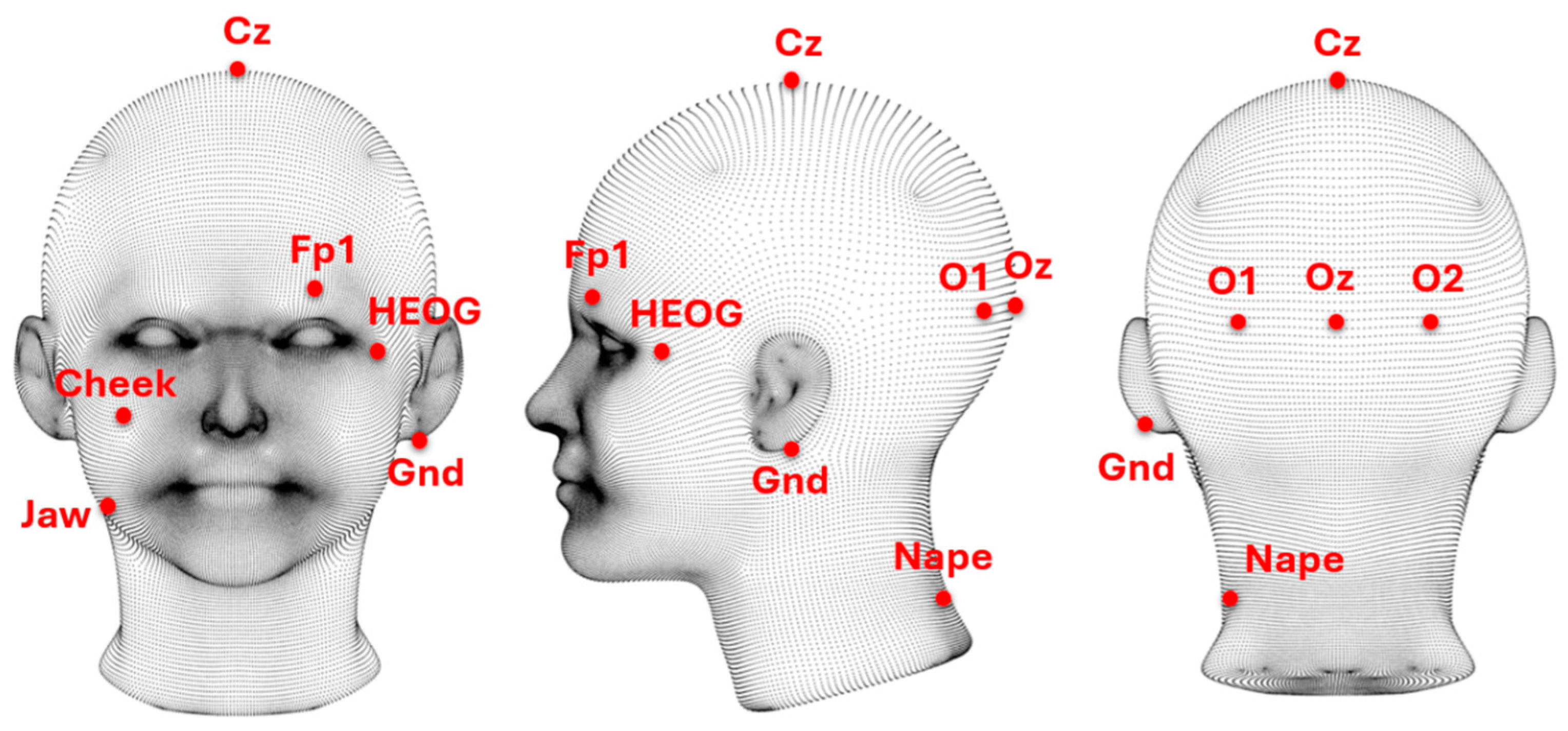
The electrodes used for data collection were selected based on earlier studies indicating the optimal configuration for recording both EEG and muscle artifacts. They included electrodes O1, O2, and Oz—associated with SSVEP—Cz and Fp1 (for EOG), and five EMG electrodes—HEOG, neck, cheek, nape, and jaw [20]. In total, nine electrodes were used in the study, along with a reference electrode attached to the participant’s earlobe. Figure 1 presents the EEG/EMG electrode placement used during the recording. The EEG electrode montage (O1, O2, Oz, Cz, and Fp1) was selected with the primary goal of optimizing the recording of SSVEP responses, while also minimizing setup time and participant discomfort. Since the experiment focused specifically on visually evoked potentials, occipital electrodes (O1, O2, and Oz) were prioritized due to their proximity to the visual cortex, where SSVEP signals are strongest and most reliably detected. Electrode Cz was added to capture the potential spread of muscle artifacts into central areas, and Fp1 served to monitor basic ocular activity such as blinking or eye movements. This configuration provided sufficient spatial resolution for the purposes of the study while reducing the time required to apply electrodes, which was particularly important when working with multiple participants. It also allowed us to maintain a clean experimental design centered on SSVEP analysis, without unnecessary complexity in channel layout. To support the identification and tracking of muscle-related artifacts, additional EMG electrodes were placed on the participant’s face and neck: HEOG, neck, cheek, nape, and jaw. These electrodes, applied using adhesive patches, enabled localized tracking of muscle activity and helped visualize the topographic distribution of non-neural interference.

During the experiment, a g.Tec g.USBamp 2.0 bioelectrical signal amplifier, an EEG cap, and a set of active g.LADYBIRD electrodes were employed. The sampling rate was set to 256 Hz. Data acquisition took place in a specially designed setup featuring an LED diode that emitted stimuli to elicit SSVEP at predefined frequencies (5–30 Hz).

Twenty-four volunteers aged 18–52 took part in the study. Each participant was informed about the procedure of the experiment both in written and oral form. After reviewing the provided information, each individual gave voluntary and informed written consent to participate in the study.

Next, each participant wore an EEG cap with active electrodes (O1, O2, Oz, Cz, and Fp1) and EMG electrodes affixed to the face and neck (HEOG, neck, cheek, nape, and jaw) using adhesive patches. A conductive gel was applied between each electrode and the skin to ensure optimal signal conduction.

A custom Matlab-based software facilitated precise data acquisition, processing, and visualization. To ensure high data quality, filtering was applied. A fourth-order Butterworth notch filter (48–52 Hz) was used to remove 50 Hz power-line interference, while an eighth-order Butterworth bandpass filter (0.5–100 Hz) was employed to preserve critical components of the brain signal. No other filters or processing methods were applied during signal acquisition.

At the beginning, each volunteer was exposed to SSVEP stimuli with frequencies ranging from 5 to 30 Hz, and real-time responses were monitored by observing the EEG spectrum at electrode O2. Responses varied among participants—some showed higher amplitudes, others lower. For each individual, the stimulation frequency associated with the strongest SSVEP response was selected based on visual inspection and expert assessment by the experiment supervisor.

Each participant completed four recording sessions, with an approximate one-minute break between sessions to allow for rest. The first session (1 min) recorded EEG/EMG signals representing brain activity free of muscle artifacts, with the participant sitting still and focusing on a non-pulsating LED. The second session (1 min) captured EEG/EMG signals in the presence of muscle artifacts (e.g., jaw clenching), with the participant sitting still but without visual stimulation. The third session (1 min) involved exposure to visual stimulation using a pulsating LED. The stimulation frequency had been selected at the beginning of the experiment to elicit the strongest SSVEP response for each participant. The fourth session (1 min) aimed to record SSVEP responses in the presence of muscle artifacts. The participant was instructed to look at a green, pulsating LED (1 cm in diameter, placed 1 m away from the eyes) while clenching their jaw to introduce muscle-related noise into the EEG signal. The experiment consisted of four 1 min sessions designed to isolate or combine SSVEP and EMG-related components.

Detailed descriptions of each session, including task instructions and expected artifacts, are provided in

Table 1. Session descriptions, task instructions, and expected artifacts.

Session	Duration	Task Description	Participant Instructions	Visual Stimulation/Muscle Artifacts
1	1 min	Recording of EEG/EMG signals without muscle artifacts. The participant sat still and focused on a non-pulsating LED.	Please sit still, relax your facial muscles, and look at the steady (non-blinking) LED in front of you.	No/No
2	1 min	Recording of EEG/EMG signals with muscle artifacts (e.g., jaw clenching), without visual stimulation.	Please sit still and gently clench your jaw for about 0.5 s, then relax it. Repeat this cycle every 2–3 s. Do not focus on any light source during this session.	No/Yes
3	1 min	Exposure to a pulsating LED at the frequency previously selected to elicit the strongest SSVEP response.	Please focus on the blinking LED and remain still, without clenching your jaw or causing any other artifacts.	Yes/No
4	1 min	Recording of SSVEP signals with simultaneous muscle artifacts (jaw clenching).	Please keep looking at the blinking green LED and gently clench your jaw for about 0.5 s, then relax it. Repeat this cycle every 2–3 s during the recording.	Yes/Yes

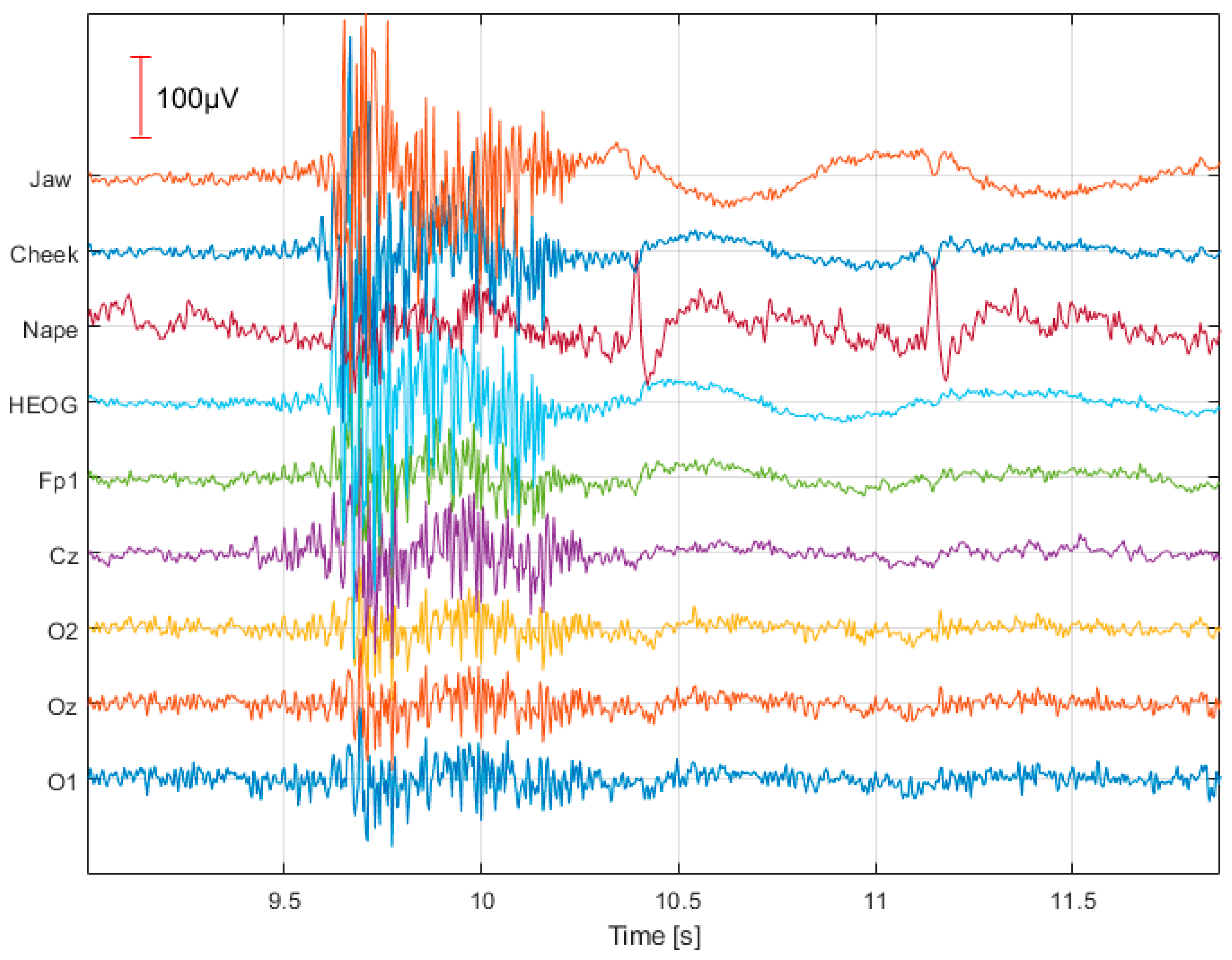
. Figure 2 shows the EEG/EMG signals recorded during jaw clenching (without visual stimulation) for participant S01. The jaw-clenching artifact occurred around 10 s, producing a substantial amplitude increase on every electrode. Notably, these artifacts also propagate to electrodes O1, O2, and Oz.

5. Methods

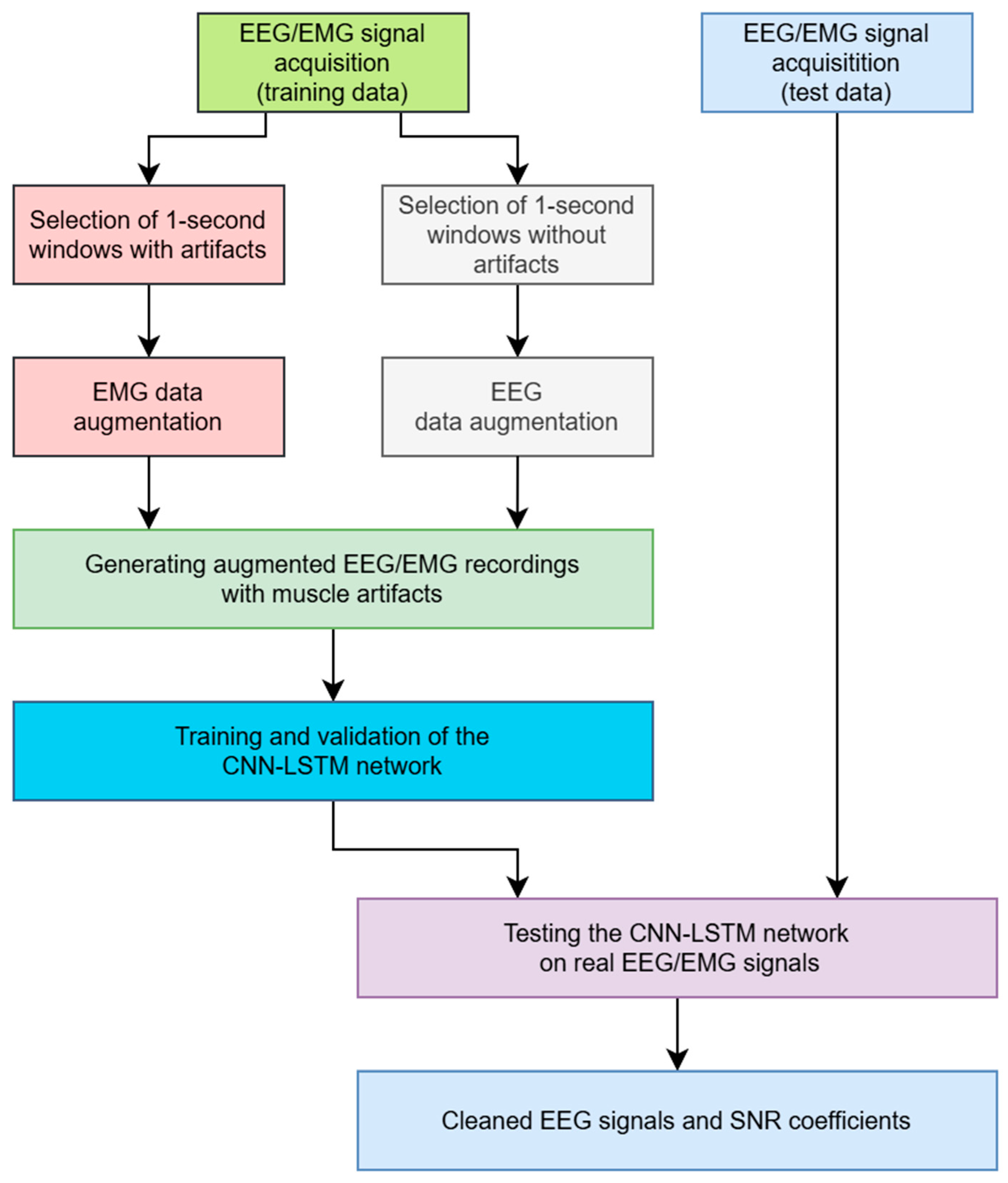
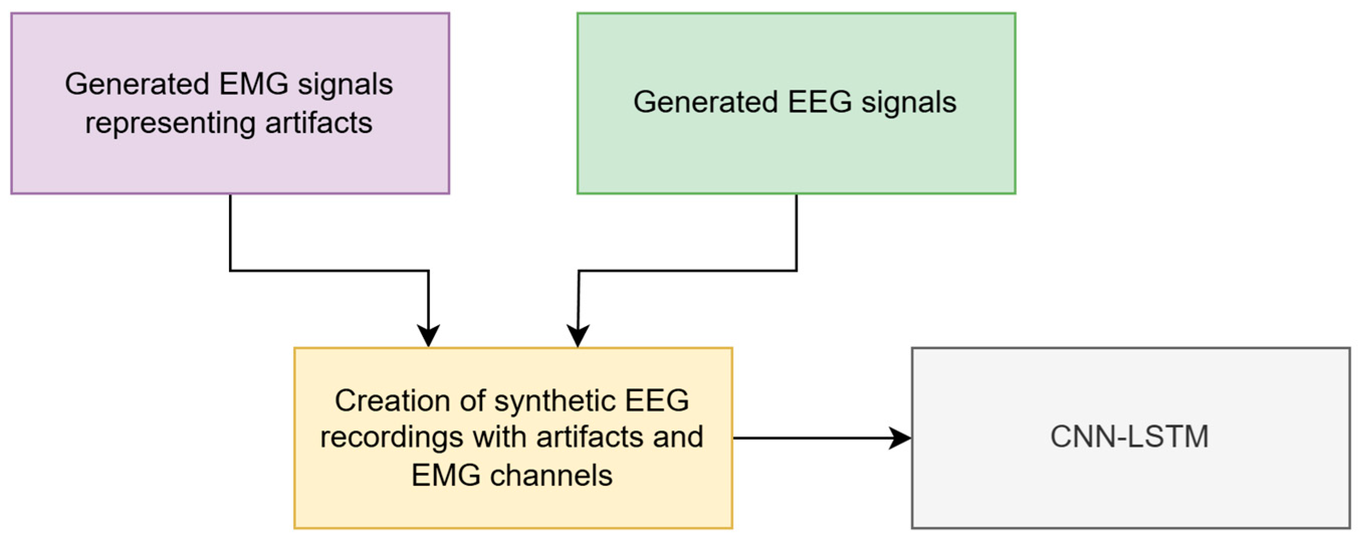
This section presents the research methods employed in the process of cleaning EEG signals from artifacts. Figure 3 illustrates the flowchart detailing the procedures employed in our study on cleaning EEG signals from muscular artifacts using a CNN-LSTM neural network. Initially, EEG and EMG signals were acquired and subsequently segmented into training data (comprising both resting sessions without stimuli and sessions with artifacts) and test data (including sessions with elicited SSVEP potentials as well as SSVEP sessions affected by muscular artifacts). To prepare the training set, we selected time windows containing muscular artifacts and artifact-free windows. For both groups, data augmentation was performed—separately for the EMG and EEG signals—to enhance the diversity and volume of the training data. The augmented dataset was then used to generate a set of synthesized EEG/EMG recordings containing muscular artifacts.

In the next stage, the CNN-LSTM neural network was trained and validated. After completing the training phase, the model was evaluated using real EEG/EMG test data. The testing phase produced cleaned EEG signals, for which the signal-to-noise ratio (SNR) coefficients were calculated as a quantitative measure of the artifact removal efficacy.

During the study, special care was taken to ensure that the same EEG signals were never used for both synthetic data generation and for training or testing the CNN-LSTM model. This approach ensured a reliable and objective evaluation of EEG signal cleaning performance under real-world conditions, without the risk of overlap between the training and testing datasets. For each user, four sessions were recorded, with the first two dedicated to data augmentation:

• EEG/EMG recordings without muscle artifacts, during which participants remained still and focused on a non-pulsating LED light source. These recordings served as a source of clean EEG samples.
• EEG/EMG recordings with muscle artifacts, such as jaw clenching, conducted without visual stimulation. These recordings were used to extract representative EMG segments containing artifacts.

The final two sessions were used to evaluate the cleaning method on real-world data:

• Exposure to a pulsating LED light at an individually selected frequency to elicit the strongest SSVEP response (clean SSVEP condition).
• Exposure to the same pulsating LED light while performing jaw clenching, introducing real muscle artifacts into the EEG signal (SSVEP + EMG condition).

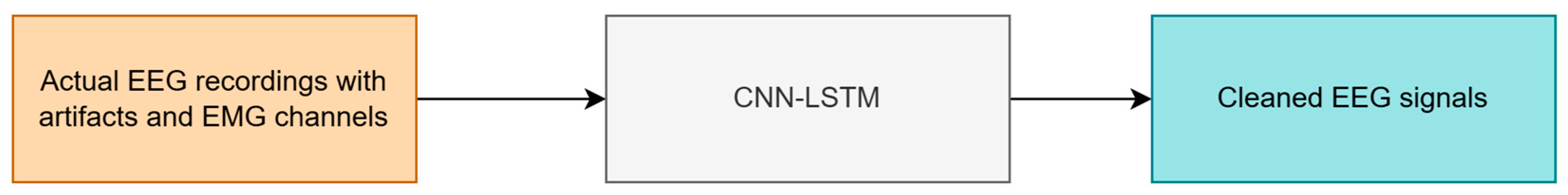
5.1. Application of CNN-LSTM for Artifact Removal

The concept of using our proposed CNN-LSTM for artifact removal is illustrated in Figure 4. The network receives input from one EEG signal channel and five additional channels that provide information about muscle activity. We assume that the CNN-LSTM outputs a single channel of cleaned EEG data, free from artifacts.

A key challenge in the presented approach was the effective training of the CNN-LSTM network. To address this, we opted to use data generated in a manner that mimics raw EEG and EMG signals. This strategy allows for the creation of a wide and diverse set of examples, essential for successful network training. To achieve this, the following steps were undertaken:

(a)

Generating EEG signals that model brain activity.

(b)

Generating EMG signals that represent muscle artifacts.

(c)

Developing augmented EEG recordings containing muscle artifacts.

Figure 5 illustrates the schematic of the EMG signal generation process and how these signals are utilized to create EEG recordings with muscle artifacts. The CNN-LSTM was trained to output clean EEG signals, free from disturbances caused by muscle artifacts. The effectiveness of the CNN-LSTM in cleaning raw EEG signals largely depends on the quality and representativeness of the training data. The augmented EEG and EMG signals created must accurately replicate the genuine properties of real signals, including their time-frequency characteristics. Additionally, it is crucial that the training data exhibit maximum diversity—for both EEG signals and muscle artifacts. Such diversity is essential as it enables the CNN-LSTM to generalize effectively and recognize various types of artifacts in raw EEG data.

5.1.1. Generation of Augmented EEG Recordings

For each participant in the study (S01–S24), a 60 s session was recorded during which the individual sat still and observed a switched-off LED with their eyes open. Under these conditions, the recorded EEG signals were assumed to be free of muscle artifacts. Next, one-second time windows were selected based on the judgment and visual assessment of a clinical neurophysiologist. The number of such artifact-free windows varied among participants, ranging from a few to several dozen.

To increase the number of artifact-free EEG examples identified by the expert, a data augmentation process was performed. Three signal-modification techniques were used to diversify the dataset in a realistic way while preserving essential signal characteristics. These techniques were spectrum modification, sample shifting, and noise addition.

The augmentation method based on spectrum modification involved randomly altering the EEG signal spectrum. Phase shifting alters the shape of the signal in the time domain, which can lead to changes in its appearance, including that of the EEG signal. However, this operation does not affect the amplitude spectrum, thereby preserving the spectral characteristics of the signal. In practice, this means that the distribution of energy across individual frequency bands remains unchanged, which is crucial for many EEG analyses based on spectral features. As a result, phase shifting can be used as a data augmentation method that enables the generation of new, diverse signal variants while maintaining their essential frequency-domain properties. First, each EEG channel was transformed using the fast Fourier transform (FFT) to analyze its spectral components. Random changes in amplitude and phase were then introduced in the frequency domain. The amplitude of each frequency component was scaled by a random factor in the range of 0.8 to 1.2, and a random phase shift between −π and π was added to each component. After these modifications, the inverse FFT (IFFT) was used to convert the spectrum back to the time domain, resulting in a modified EEG signal.

The augmentation method using sample shifting involved randomly and cyclically shifting the EEG signal in time. An offset between −100 and 100 samples was selected randomly. The signal was then shifted accordingly, with samples exiting from one end and re-entering at the other end in a first-in–first-out manner. This approach maintained data integrity while introducing variability in the time domain, thus enriching the training set.

The augmentation method involving noise addition introduced random Gaussian noise to simulate real-world measurement conditions, where interference naturally occurs. First, Gaussian noise was generated and scaled relative to the standard deviation of the EEG signal, at 5% of that standard deviation. The noise was then added to the EEG signal, introducing subtle distortions that resembled actual recording conditions.

By employing these augmentation techniques, a diverse dataset was created that closely mirrored the properties of raw EEG signals while also increasing the dataset’s size and variety. This provided a solid foundation for training and testing neural network models. Each of the techniques was applied separately. In total, 80,000 EEG signals were generated through these augmentation methods. A visual inspection of several dozen randomly chosen augmented EEG samples confirmed that they closely resembled raw EEG recordings.

5.1.2. Generation of Augmented EMG Recordings

An analogous approach was used for generating augmented EMG signals as for EEG signals. However, in this case, the primary objective was to replicate muscle-origin interference. EMG signals recorded during participants’ muscle activity served as templates for artifacts, specifically those captured from jaw clenching. To ensure high-quality output, a clinical neurophysiologist performed a visual assessment of one-second time windows and selected those segments that best represented muscle interference. This process yielded examples most characteristic of EMG artifacts, with the number of selected windows varying among users—ranging from a few to several dozen.

The data augmentation process involved operations such as adding random noise, shifting signals in time, and modifying their spectral properties. Through this approach, a rich set of EMG signals was produced, accurately reflecting the muscle interference observed under real recording conditions. A visual inspection of several dozen randomly chosen augmented EMG signals confirmed that they closely resembled actual recorded EMG signals.

5.1.3. Generating Augmented EEG Recordings with Muscle Artifacts

The method of generating augmented EEG recordings with added EMG artifacts enables the creation of controlled yet realistic conditions for evaluating and refining algorithms designed to remove muscle interference. To achieve this, the generated EEG and EMG signals are utilized. EMG artifacts undergo random amplitude scaling and random time shifting. During the scaling stage, the artifact is multiplied by a random factor (ranging from 0.5 to 1) to adjust its amplitude to the desired values. The positioning stage determines the point in the EEG signal at which the artifact will be introduced. This can be any location within the signal. Next, the generated EMG artifacts are added to the generated EEG recording, resulting in an EEG signal corrupted by muscle artifacts.

The process of synthetic data generation involves all 6 signal channels—1 EEG channel and 5 EMG channels. Both the amplitudes of individual artifacts and the weights used to combine them were randomly selected for each generated sample. As a result, a high level of variability was achieved in terms of the type, intensity, and distribution of artifacts in the signals. This approach enables the creation of realistic and diverse data, which is crucial for effectively training the denoising model. A visual inspection of several dozen randomly selected augmented signals confirmed that they resemble real signals. 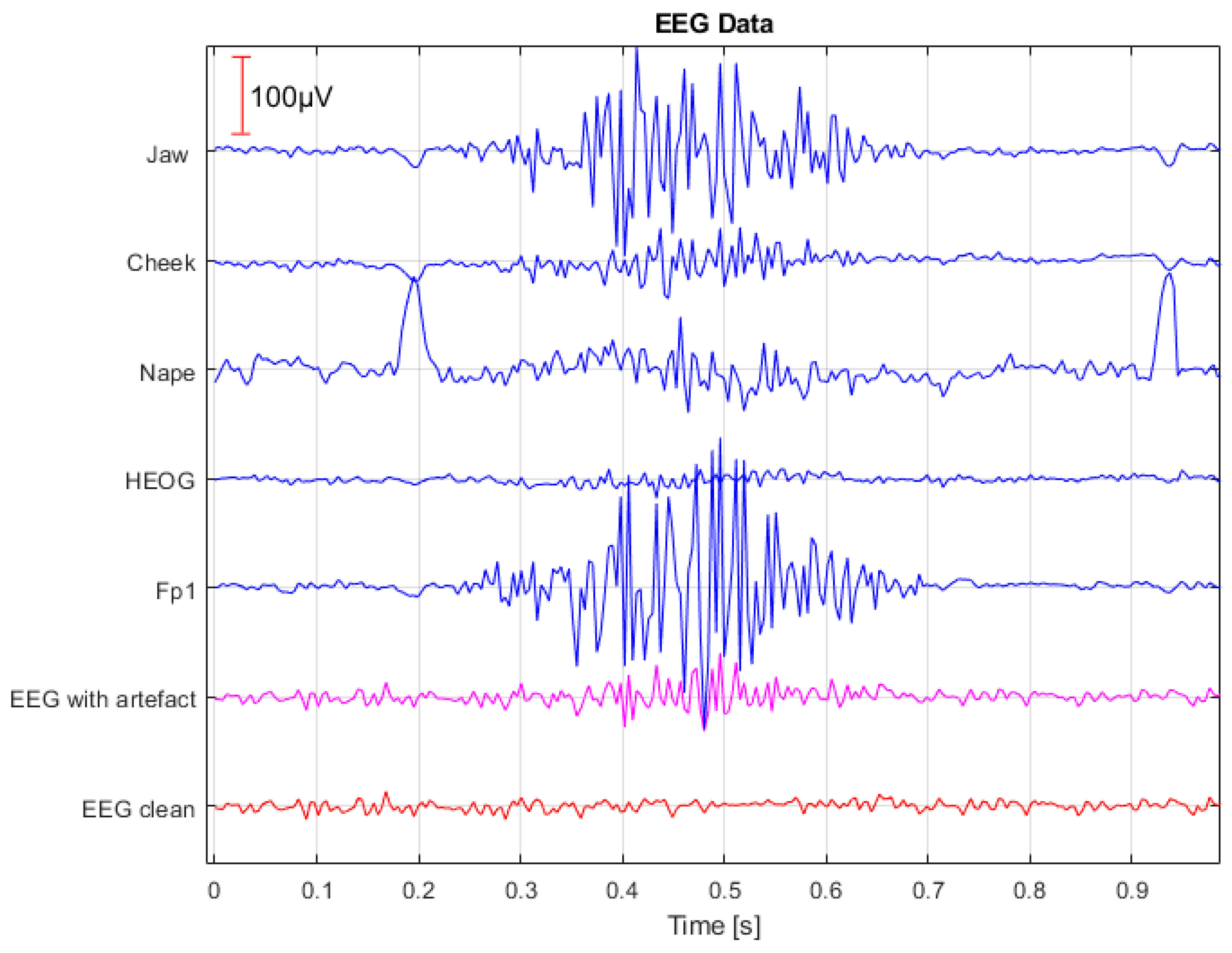Figure 6 presents sample EEG and EMG signals generated for training a CNN. Artifacts originating from the Fp1, HEOG, nape, cheek, and jaw electrodes are highlighted in blue. The EEG signal containing these artifacts is shown in magenta, while the artifact-free EEG signal is depicted in red. The generated dataset has been made available in the EEG/EMG database on the website: https://dx.doi.org/10.21227/c4k4-zd80 (accessed on 25 April 2025).

Through this approach, we have a dataset containing both clean EEG signals and EEG signals contaminated with muscle artifacts, allowing for a reliable assessment of artifact detection and filtering methods. It also provides a rich training resource for machine learning models. During the generation process, no attempt was made to reflect SSVEP.

5.1.4. Proposed CNN-LSTM Structure and Training

The proposed CNN-LSTM architecture is presented in

Table 2. Structure of the proposed CNN-LSTM.

Layer	Parameters	Input Size	Output	Number of Parameters
Input	Input containing signals with artifacts. A matrix of 256 samples per 6 EEG/EMG channels is fed to the network.	(256, 6, 1)	(256, 6, 1)	-
Conv2D	128 filters of size [1, 6], padding “valid”, and ReLU activation function.	(256, 6, 1)	(256, 1, 128)	896
Conv1D	256 filters of size 1, padding “valid”, and ReLU activation function.	(256, 1, 128)	(256, 1, 256)	33,024
Reshape	Prepares data for sequential analysis in the LSTM layer.	(256, 1, 256)	(256, 256)	-
LSTM	256 LSTM units, gate activation—sigmoid function, and state calculation—hyperbolic tangent.	(256, 256)	(256, 256)	525,312
Flatten	Converts data into a one-dimensional feature vector for the Dense layer.	(256, 256)	(65 536)	-
Dense	Number of neurons 256, linear activation function.	(65 536)	(256, 1)	16,777,472

. The network architecture was selected based on a series of ablation experiments, in which we tested different numbers of filters (32, 64, 128, 256, and 512) in the Conv2D, Conv1D, and LSTM layers. The primary selection criterion was the validation error (MSE), but it was not the only one. During model selection, we also assessed the quality of the cleaned EEG signals—both visually and in the frequency domain. Particular attention was paid to segments of the signal that did not contain artifacts, as it was essential that the network did not introduce distortions where no noise was present. Additionally, we considered various architectural variants, including models based solely on CNN layers, only on LSTM layers, and their combinations. The final model was chosen based on its ability to effectively remove artifacts while preserving the structure of the original signal.

A matrix of 256 samples by 6 channels is fed into the network input. This corresponds to 1 s of data for the EEG channel that we aim to clean of artifacts, along with 5 additional channels capturing muscle activity (Fp1, HEOG, neck, cheek, nape, and jaw). The next layer is a two-dimensional convolutional layer (Conv2D). Its primary role is to analyze the relationships between the EEG and EMG samples. This layer uses filters with dimensions of 1 × 6. Such filters represent a linear combination of samples at the same point in time across the different channels, analogous to operations like Laplacian spatial filters, common average reference (CAR) filters, or common spatial pattern filters. By doing so, the network can capture shared signal features from multiple channels, which may indicate the presence of artifacts. ReLU activation (rectified linear unit) introduces nonlinearity and helps the network learn complex relationships in the data while accelerating the training process by mitigating the vanishing gradient problem.

Another important part of the network is the one-dimensional convolutional layer (Conv1D), which operates on the data processed by the Conv2D layer. The main goal of this layer is to amplify and extract samples in the EEG signal at the individual time-point level. Using the ReLU activation function here as well further enhances modeling performance and speeds up training. The output of this layer provides more detailed information on local changes in the EEG signal. After the Conv1D layer, the data is passed to a Reshape layer, which transforms the data into a format suitable for temporal analysis in the LSTM layer. The Reshape layer flattens the spatial dimensions while retaining the time information, a crucial step for subsequent analysis. The proposed approach allows spatial dependencies between channels to be encoded at the level of the first convolutional layer, which processes all channels simultaneously. These dependencies are not further processed in their original spatial form but are instead transformed into feature representations that are passed to the LSTM layer as temporal input. Although the explicit spatial structure is no longer preserved after the Reshape operation, we assume that relevant inter-channel patterns are captured during the early stages of processing and remain available in the subsequent layers of the network.

A key component of the network is the LSTM (long short-term memory) layer, which analyzes temporal dependencies in the EEG data. LSTM is a specialized form of recurrent neural network that retains information about previous samples and incorporates that information when processing subsequent time points. Since EEG signals are sequential, the LSTM layer enables the model to capture long-term temporal relationships, including phase relations in the signal. This makes LSTM particularly effective for examining the dynamic processes occurring in biological signals.

The Flatten layer transforms the LSTM output into a one-dimensional vector. This operation is necessary so that the data can be processed by the fully connected Dense layer that follows. By flattening, all features are combined into a single vector suitable for predicting the cleaned EEG signal. Finally, the network includes a fully connected Dense layer acting as a regression layer to predict the artifact-free EEG signal. This layer uses a linear activation function, allowing for the prediction of continuous values. Its output represents the cleaned EEG signal. The output vector of the model with dimensions (256, 1) corresponds to the cleaned EEG signal from a single channel. It refers to a specific time window from the input signal and represents the signal after artifact removal by the model. The total number of network parameters is 17,336,704.

For training the model, the ADAM (adaptive moment estimation) algorithm was used. ADAM dynamically adjusts the learning rates for each weight in the neural network and combines the advantages of two popular optimization methods—RMSProp and momentum. As a result, it enables rapid and stable convergence, even with large datasets and complex models. ADAM is widely employed in CNN and LSTM training tasks. In the machine learning process, several key parameters in the ADAM algorithm influence how the model weights are updated. The learning rate was set to 0.001, determining the step size for weight updates and thus the model’s rate of adaptation. A decay of 0.0 means that there was no reduction in the learning rate during training. The beta_1 parameter was set to 0.9, smoothing the first moment by calculating the moving average of gradients, while beta_2 was set to 0.999, smoothing the second moment by considering the moving variance of gradients. A small epsilon value of 1 × 10⁻⁷ was used for numerical stability. The AMSGrad algorithm was not utilized, so the default ADAM approach was retained. These configurations were used throughout the training process.

The model’s loss function was mean squared error (MSE), which measures the difference between the predicted (artifact-removed) signal and the true artifact-free EEG signal provided by the generator. Minimizing the MSE ensures that the model accurately reconstructs the target signal, thus effectively removing artifacts from the EEG recordings. A dataset of 80,000 generated examples was prepared for training the neural network. The data were split into three subsets: training (70%), validation (15%), and testing (15%).

Table 3. Splitting the dataset into training, validation, and test sets.

Data Subset	Number of Examples	Description
Training	56,000	A total of 70% of the data to optimize network weights during training.
Validation	12,000	A total of 15% of data used to monitor model performance.
Test	12,000	A total of 15% of data for model quality assessment after training.

provides details about how the data were divided.

Training was conducted using batches of size 32. This choice balanced training speed with the stability of the optimization process. The model was trained for a maximum of 50 epochs. An early stopping mechanism was implemented, monitoring the loss on the validation set, with a patience of 3 epochs. The algorithm stopped at the 7th epoch, where the MSE was 0.092 for the training data and 0.211 for the validation data. To improve generalization and robustness, data augmentation was applied by injecting diverse and intensified synthetic artifacts—stronger and more varied than real EEG disturbances. This helped the model learn to generalize across a wider spectrum of potential noise. Training results were stable across different random weight initializations. After training, the MSE on the test data was 0.189, indicating a properly executed training process and acceptable generalization performance, especially considering the complexity and variability of EEG signals. Importantly, visual and spectral analysis confirmed that the model did not introduce distortions in clean signal segments, which is critical for reliable artifact removal.

5.2. Linear Regression Applied to Artifact Elimination

Linear regression was the second algorithm used by us to remove muscle artifacts from EEG signals. This approach models the relationship between reference signals, such as EMG, and the recorded EEG signal. EMG signals serve as indicators of interference, which are then subtracted from the EEG signal based on the calculated regression coefficients. According to [21], regression methods were frequently used in the 1990s to remove EOG artifacts due to their simplicity and low computational demands. They remain popular and widely used for artifact removal to this day [21]. The technique requires one or more electrodes, referred to as reference electrodes, dedicated to recording interference. These are often placed near the eyes or muscles to capture EOG and EMG artifacts for subsequent removal. Linear regression assumes that each EEG recording channel is the sum of an uncontaminated source signal (neuronal activity) and a linear combination of the reference signals [22]. Neuronal activity is considered independent of the reference electrodes. The goal of regression is to estimate the optimal propagation coefficient for each reference electrode using the least squares method. The correction of a contaminated EEG signal is performed by subtracting a weighted portion of the reference signal from the contaminated EEG, resulting in a cleaned signal.

Regression for EEG signal cleaning has several significant advantages, making it a popular tool in neurophysiological data analysis. First, it is a straightforward, computationally efficient method that does not require advanced algorithms. Consequently, it is fast and easy to implement. Despite these strengths, regression also has certain limitations. One of the main assumptions is that artifacts are a linear combination of signals from the reference electrodes, which can be a constraint. In reality, artifacts may be more complex and nonlinear, making regression insufficient in such cases for effective signal cleaning.

Using regression to remove artifacts requires the careful selection of reference electrodes, ensuring that these electrodes contain only artifacts rather than neuronal signal components. Regression remains an effective method for cleaning EEG signals and is still used today, particularly when fast, real-time calculations are needed (e.g., in BCI).

In our study, all EMG/EOG electrodes (HEOG, neck, cheek, and jaw) were used as reference electrodes. Cleaning focused on signals from the electrodes most commonly used in BCI—O1, Oz, O2, and Cz. Each electrode was cleaned sequentially using the reference channels. Regression was performed in time windows rather than applied once to the entire dataset, meaning the regression model operated on smaller, shifting segments of data (windows), allowing local temporal relationships and variability to be taken into account. The window length was experimentally set to 1 s (256 samples). A wider window would contain multiple artifacts as well as artifact-free signal segments, while a narrower window might not capture individual artifacts.

5.3. Independent Component Analysis for Artifact Removal

The third algorithm we implemented, which was used to separate and remove muscle artifacts from the EEG signals, was independent component analysis. This technique decomposes the EEG recordings into independent components, some of which may be associated with EMG artifacts. Once these artifact-related components have been identified, they are discarded, and the remaining signals are reconstructed to obtain a cleaned EEG signal.

ICA is a popular method for cleaning EEG data. Its primary advantage lies in its ability to separate the signal into independent components without the need for artifact indicator channels [22,23]. As a result, ICA is often used in situations where artifacts cannot easily be modeled through methods requiring artifact indicator channels. The goal of ICA is to decompose the signals recorded by each electrode into independent components, the number of which is specified by the user but typically does not exceed the number of electrodes used in the recording. In principle, among these components are those responsible for noise sources (artifacts such as blinking, muscle tension, ECG interference, etc.). Components containing artifacts are discarded either automatically or by an expert, and the remaining components are recombined via the ICA mixing matrix to yield artifact-free signals. A critical step in the ICA algorithm is whitening, which transforms the data so that they have a unit variance and are mutually uncorrelated. This process simplifies solving the source separation problem by eliminating correlations between components. In practice, it means that before running ICA, the EEG signals are transformed into a form in which their correlation coefficients are zero.

Among the assumptions of ICA [3] is that the source signals are statistically independent. This means that the signals representing both noise sources (artifacts) and neuronal activity must be statistically independent so that their statistics (mean, variance, skewness, and kurtosis) are uncorrelated. Additionally, the model allows for at most one normally (Gaussian) distributed source signal [3]. After applying ICA to the recorded signals, one obtains the requested number of independent components, each potentially corresponding to neuronal activity or artifacts. To remove artifacts, one identifies the components responsible for the interference and sets them to zero. The final signal is then reconstructed from the remaining components using the modified mixing matrix.

One of ICA’s main benefits is that it does not require artifact indicator channels. Unlike regression, ICA does not need predefined artifact indicator electrodes, which can be a significant advantage when artifacts may originate from different locations or multiple indicator electrodes would be required. This method is particularly useful when no suitable indicator electrodes are available or when setting them up would be difficult. Another notable strength of ICA is its effectiveness in separating signal sources. It can effectively isolate components related to artifacts (e.g., blinking, muscle tension, or ECG interference) from those reflecting neuronal activity, allowing the removal of unwanted artifacts without affecting the valuable brain signals. By doing so, ICA reduces the impact of artifacts on subsequent EEG analyses, retaining only clean neural activity. Furthermore, ICA is highly versatile and can be applied to various types of artifacts, including eye movements, muscle tension, ECG, and other interferences.

Despite its advantages, ICA has some limitations. One important consideration is the assumption of statistical independence among source signals. While neuronal activity can sometimes correlate with certain artifacts, ICA can still effectively separate overlapping signals if they differ in spatial topography or temporal dynamics. The main challenge in such cases is often not the separation itself, but rather the correct identification and interpretation of the resulting components. Another known limitation is that ICA performs poorly when attempting to separate components that follow similar Gaussian distributions. Although this is a theoretical constraint, in practice many neural and artifact-related sources are sufficiently non-Gaussian, allowing ICA to perform well in real-world EEG applications. Finally, even when ICA correctly isolates artifact components, distinguishing them from brain-related activity can be difficult—especially when their features are subtle or overlap in spectral content or scalp distribution. In such cases, expert review or dedicated algorithms are required to guide the removal process. Incorrectly discarding components may result in either insufficient artifact removal or the loss of neural signals.

As demonstrated in [24], rank deficiency can negatively affect the performance of ICA. Therefore, prior to ICA decomposition, the rank of the preprocessed data from each session was verified to ensure that full rank was preserved. No rank deficiency was observed, and ICA was applied without compromising data rank.

In this study, the well-known and widely used FastICA [25] algorithm was employed, with the number of components set to match the number of channels in the data. Default function parameters were used. The hyperbolic log function (logcosh) was chosen to measure departures from normality, offering a suitable balance of performance and speed in standard applications. The algorithm was run for a maximum of 200 iterations, providing sufficient steps to ensure convergence, with a tolerance of 0.0001 to achieve accurate results without excessive computation time. The initial matrix for separating signals was generated randomly, allowing the algorithm to start with neutral assumptions.

Artifact components were discarded by means of visual inspection, involving the manual evaluation of the component contents and their impact on the signal. This procedure was performed over the entire duration of the recorded signal.

6. Results and Discussion

6.1. Comparison of Augmented and Real Signals

To assess the quality of the augmented data, we compared basic statistics between EEG signals acquired from real recordings and those generated by the simulator.

Table 4. Comparison of real and augmented EEG signals.

Channel	Mean (Real) [µV]	Mean (Aug) [µV]	Std Dev (Real) [µV]	Std Dev (Aug) [µV]	Skewness (Real) [-]	Skewness (Aug) [-]	Kurtosis (Real) [-]	Kurtosis (Aug) [-]
Raw EEG (clean)	0.022	0.26	9.24	9.65	0.09	0.24	2.4	2.97
EEG (artefact)	−0.77	1.8	24.17	34.7	0.09	0.16	5.4	5.5
Fp1	−2.23	1.53	97.67	60.25	−0.44	0.08	11.0	10.9
HEOG	−0.03	1.19	38.6	59.51	−0.1	−0.03	6.1	11.02
Nape	−0.83	5.33	30.31	91.02	1.21	0.33	5.7	6.92
Cheek	−1.2	1.36	43.63	63.51	0.36	−0.02	6.5	11.25
Jaw	−1.83	−1.81	72.28	61.65	0.09	−0.02	3.0	10.97

summarizes the mean values, standard deviations, skewness, and kurtosis for the clean signals, artifact-contaminated signals, and individual channels. The results indicate an overall similarity in the statistical characteristics of the real (real) and augmented (aug) signals. For example, for clean EEG, the mean was 0.02 µV compared to 0.26 µV for the augmented version, with standard deviations of 9.24 µV and 9.65 µV, respectively. In the EEG channel with artifacts, the mean values were −0.77 µV and 1.80 µV, and the standard deviations were 24.17 µV and 34.70 µV for the real and augmented signals, respectively. Skewness and kurtosis measures were also similar; for instance, for the artifact-affected channel, skewness values were 0.09 and 0.16, while kurtosis values were 5.4 and 5.5. Despite some local differences across individual channels, the augmented data exhibit an overall distribution consistent with the real data, confirming their suitability for further analysis and EEG signal modeling.

6.2. Assessment of Artifact-Induced Disruption of SSVEP

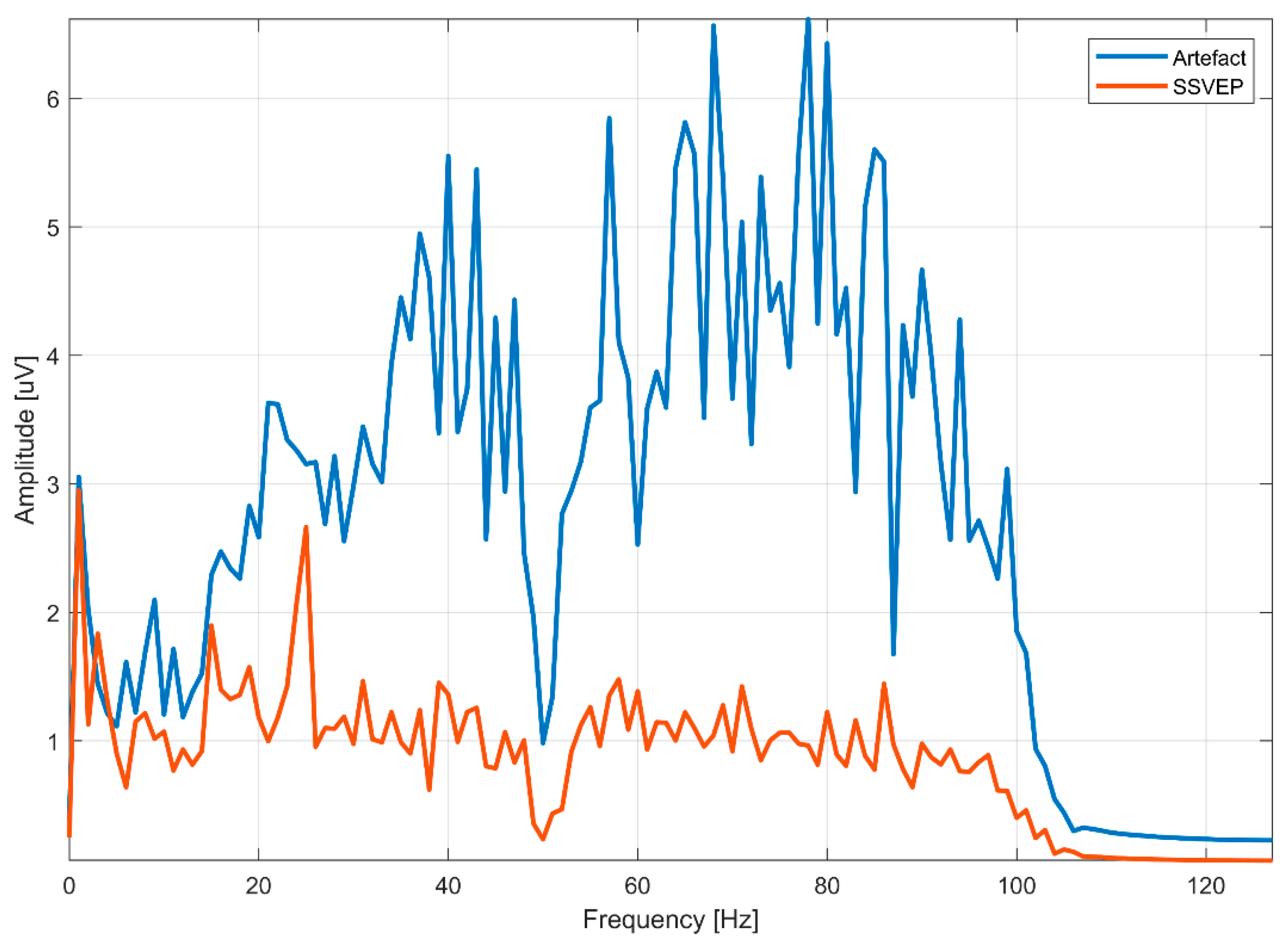
As a first step, it was verified whether the jaw clenching artifact actually disrupts SSVEP. For this purpose, during stimulation at the frequency of 25 Hz, 10 windows with artifacts and 10 windows without artifacts were selected. Figure 7 presents the signal spectrum at electrode O2 for participant S24, comparing artifact-free time windows with windows containing muscle artifacts. In both cases, steady-state visually evoked potentials were elicited at 25 Hz. As shown, jaw-clenching artifacts severely disrupt the SSVEP signal, preventing effective detection. This underscores the importance of thorough EEG preprocessing to remove artifacts.

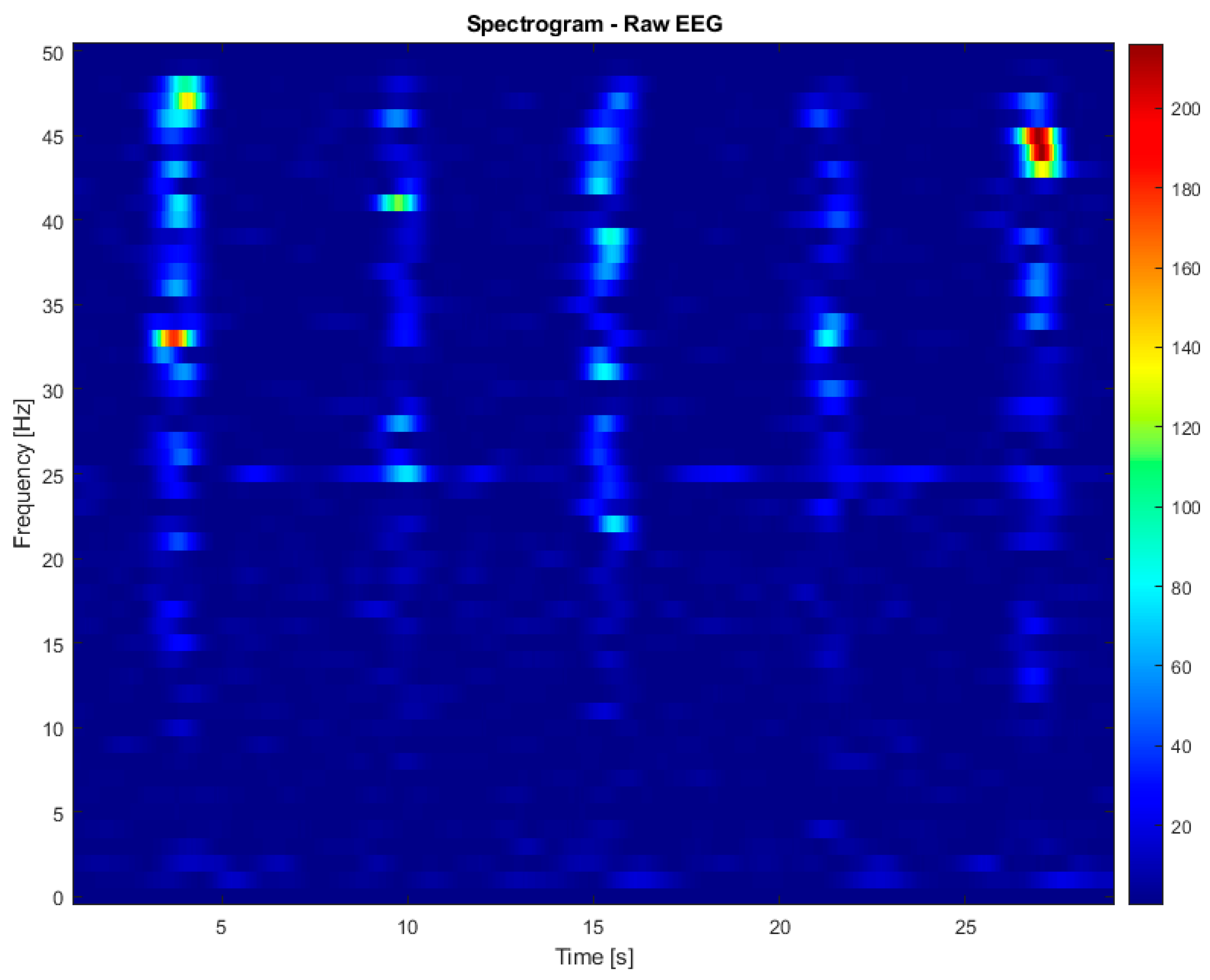
Figure 8 illustrates the spectrogram of EEG signals recorded during stimulation at the frequency of 25 Hz during jaw clenching at 4, 10, 16, 22, and 27 s, also recorded from participant S24 at electrode O2. For most of the recording, 25 Hz SSVEP is clearly visible. However, during jaw clenching, muscle activity strongly propagates to O2 and disturbs the 25 Hz frequency associated with the SSVEP. Similar trends were observed in other participants. At lower stimulation frequencies (5–20 Hz), these artifacts were less disruptive to SSVEP than at higher frequencies (>20 Hz).

6.3. Visual Evaluation of EEG Signal Cleaning Quality

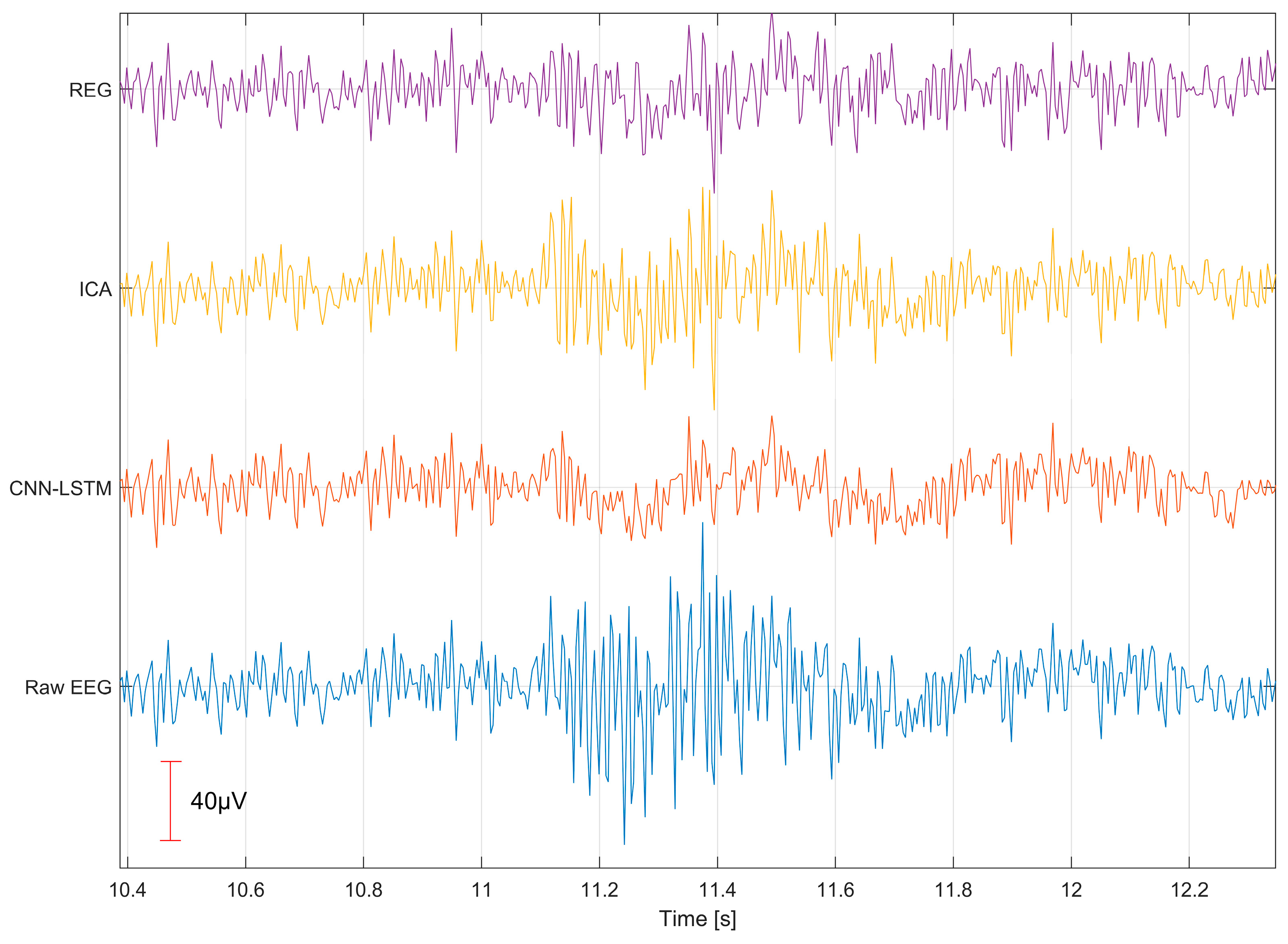
In this study, three techniques were used to clean the EEG signals from electrodes O1, O2, Oz, and Cz: regression, independent component analysis, and a CNN-LSTM neural network. The goal was to remove interference caused by EMG muscle artifacts. Figure 9 shows examples of EEG signals at electrode O2 in the time domain before and after each cleaning method for participant S2, illustrating the differences between the original and cleaned signals. Compared to the raw EEG, each method reduced the signal amplitude during the artifact periods. Notably, the CNN-LSTM method achieved the greatest amplitude reduction during the artifact intervals, while regression (REG) and ICA yielded slightly higher amplitudes. Nonetheless, all methods preserved a cleaned signal that closely resembled the original. Similar results were observed for other participants.

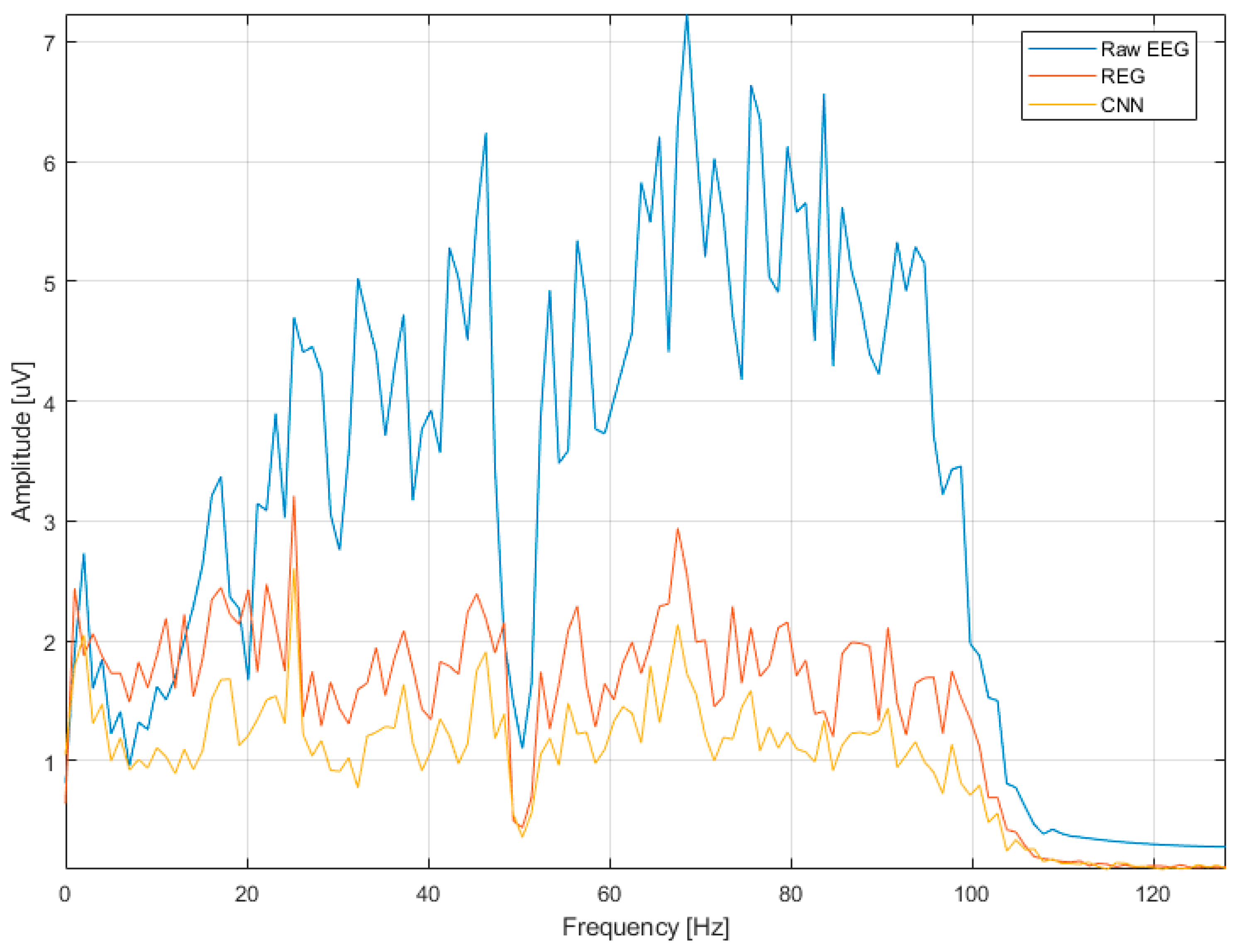
Figure 10 illustrates the EEG spectra before and after cleaning using the REG and CNN-LSTM methods, showing interference reduction in selected frequency bands. These methods were the only ones that enabled moderate artifact removal while preserving SSVEP. A 25 Hz peak can be seen in the spectrum for both REG and CNN-LSTM.

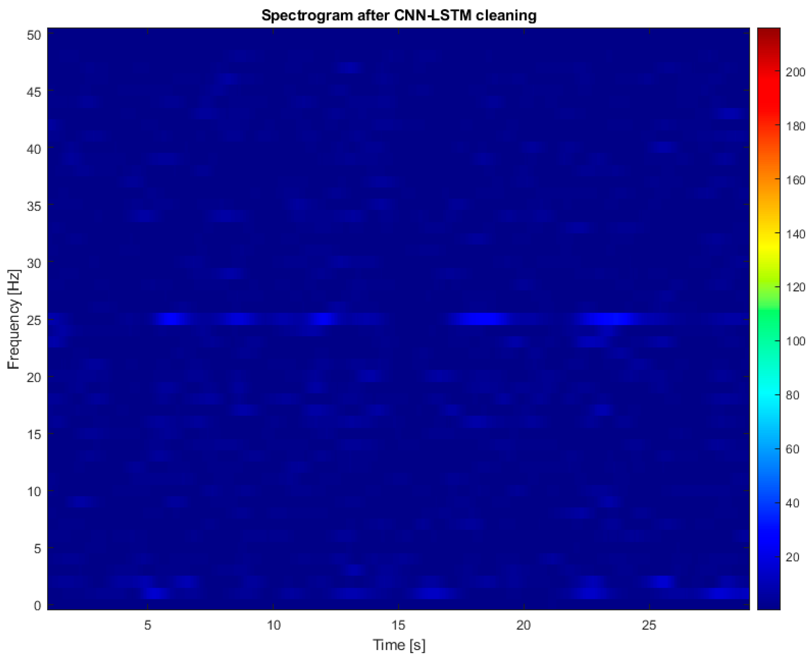
In the ICA method, a clinical neurophysiologist selected the components to remove. In many cases, it was not possible to choose only the components related to noise. As a result, the removed components also contained EEG signals and SSVEP. This made the SSVEP results inconsistent and dependent on the expert’s subjective judgment. Figure 11 shows the spectrogram after artifact removal using the CNN-LSTM method for participant S24 at electrode O2. Compared to Figure 8, the artifact-related interference has been eliminated, and the 25 Hz SSVEP is still visible. Figure 12 presents the difference in spectrograms between the original signal and the signal cleaned with CNN-LSTM. It can be seen that the CNN-LSTM method removed the artifact activity at seconds 4, 10, 16, 22, and 27. Notably, CNN-LSTM did not remove the 25 Hz frequency, indicating that the SSVEP was preserved.

6.4. Evaluation of EEG Signal Cleaning Methods Using SNR Coefficient

To evaluate the efficiency of EEG signal cleaning, a measure was proposed that expresses the ratio of the SSVEP signal amplitude at the SSVEP frequency to the average amplitude of the EEG signal frequencies in the 1–100 Hz range. This ratio can be defined as follows:

$${\mathrm{SNR}}_{\mathrm{SSVEP}}={\displaystyle \frac{A_{\mathrm{SSVEP}}}{A_{\mathrm{EEG}}}}$$

(1)

where A_SSVEP is the amplitude of the signal at the characteristic SSVEP frequency, determined from the spectrum using the Fourier transform as $\left|FFT\left(f_{base}\right)\right|$, with $f_{base}$ representing the stimulation frequency. A_EEG is the average amplitude of the EEG signal in the 1–100 Hz range, calculated as follows:

$$A_{\mathrm{EEG}}={\displaystyle \frac{1}{N}}\sum _{f=1}^{100}\left|FFT\left(f\right)\right|$$

(2)

Here, |FFT(f)| is the amplitude of the signal spectrum at frequency f, and N is the number of frequency lines within the 1–100 Hz range (in this case, N = 100).

A high SNR_SSVEP value implies that the SSVEP signal stands out markedly against the rest of the EEG activity, indicating a strong presence of the SSVEP. Conversely, a low value for this metric suggests the SSVEP is less discernible against the EEG background, indicating limited effectiveness of the particular method. For the original EEG signals, this coefficient is generally low since the SSVEP frequency is overshadowed by muscle-artifact activity. By using SNR_SSVEP, it becomes possible to quantitatively compare various EEG processing methods with regard to their ability to extract SSVEP signals, even in the presence of interference or artifacts.

Table 5. SNR_SSVEP calculated for one-second time windows that contain jaw-clenching artifacts, selected during stimulation with jaw clenching, for electrode O2.

Subject	Stimulus Frequency	Raw EEG	CNN-LSTM	REG	ICA
S01	7	1.195	2.387	2.213	1.662
S02	7	0.583	1.194	0.775	0.933
S03	6	1.495	2.019	2.028	1.615
S04	7	1.613	2.440	1.875	1.642
S05	8	0.936	1.403	1.116	1.092
S06	8	0.776	1.893	1.278	1.123
S07	7	1.092	2.053	1.730	1.421
S08	8	0.798	1.689	1.537	1.182
S09	6	1.231	2.073	1.752	1.422
S10	6	0.779	1.521	1.284	1.163
S11	6	1.047	1.902	1.483	1.310
S12	6	2.007	2.743	2.670	2.185
S13	7	1.314	2.266	2.070	1.688
S14	8	0.867	1.459	1.210	1.081
S15	6	0.924	2.403	1.352	1.131
S16	7	0.990	2.499	2.431	1.458
S17	8	0.860	2.230	2.115	1.267
S18	7	1.535	2.513	2.288	1.554
S19	8	2.882	4.806	4.735	3.833
S20	7	0.925	1.556	1.458	1.104
S21	8	1.409	2.067	2.072	1.592
S22	25	1.139	2.034	1.963	1.827
S23	25	0.711	1.475	1.425	0.686
S24	25	1.050	1.725	1.465	1.114
Mean		1.173	2.098	1.847	1.462
Std		0.482	0.694	0.753	0.589

shows the SNR_SSVEP values calculated for one-second time windows that contain jaw-clenching artifacts, selected during stimulation while jaw clenching. The analysis was performed for different signal processing methods: the original EEG (raw EEG), regression-based artifact removal (REG), the CNN-LSTM-based approach, and independent component analysis, focusing on the O2 channel. Each of these methods aims to improve the quality of the EEG signal, which is reflected in higher SNR_SSVEP values. Higher values indicate more effective extraction of SSVEP and better suppression of artifact influence. The SNR_SSVEP values for the original EEG signals serve as a baseline for comparing the effectiveness of the individual methods. From the presented results, one can observe how different EEG processing approaches handle the reduction of artifact influence and the enhancement of the useful SSVEP signal. These values allow for an assessment of which method most effectively improves the quality of SSVEP detection under challenging interference conditions.

Analysis showed that the CNN-LSTM method achieved the highest average SNR_SSVEP (2.098), indicating its effectiveness in enhancing the SSVEP signal against interference. The REG method, with an average SNR_SSVEP value 1.847, ranked second in terms of efficiency. The ICA method (1.462) demonstrated a moderate improvement in the SNR. For the original EEG signal (raw EEG), the average SNR_SSVEP was 1.173, serving as a baseline for assessing the effectiveness of the processing methods.

Statistical analysis comparing the effectiveness of different EEG processing methods revealed significant differences between the approaches. Paired-sample t-tests showed that the differences between methods were statistically significant (p < 0.001), indicating that the observed effects are unlikely to be due to chance. Specifically, all processing methods—CNN-LSTM, REG, and ICA—significantly outperformed the raw EEG signals. Furthermore, CNN-LSTM produced significantly higher values than both REG and ICA, suggesting it was the most effective method in this dataset. REG also significantly outperformed ICA, confirming its greater improvement over raw data. In summary, all pairwise comparisons between methods yielded statistically significant differences (p < 0.001), with CNN-LSTM achieving the best overall performance.

We obtained very similar SNR values for artifact removal in channels O1 and Oz, confirming that the algorithm performs well for these electrodes and may have practical applications in BCI systems.

The SNR_SSVEP alone is not sufficient for evaluating the effectiveness of artifact removal methods. It is possible that, in addition to eliminating interference, a given method may also modify useful EEG signal characteristics—that is, it may remove desired components along with the artifacts. Therefore, in addition to assessing SNR_SSVEP improvement, it is valuable to compare how each method affects signal segments containing artifacts versus artifact-free segments. For this purpose, an analysis of SNR_SSVEP was performed for each method separately, considering one-second EEG signal windows containing artifacts and clean segments. The results are summarized in

Table 6. SNR_SSVEP for EEG signals with and without artifacts, calculated for one-second time windows containing jaw-clenching artifacts at electrode O2.

	EEG Signal Without Artifacts				EEG Signal with Artifacts
	Raw EEG	CNN-LSTM	REG	ICA	Raw EEG	CNN-LSTM	REG	ICA
mean	2.475	2.653	2.725	2.701	1.173	2.098	1.847	1.462
std	0.860	0.927	1.004	0.948	0.482	0.694	0.753	0.589

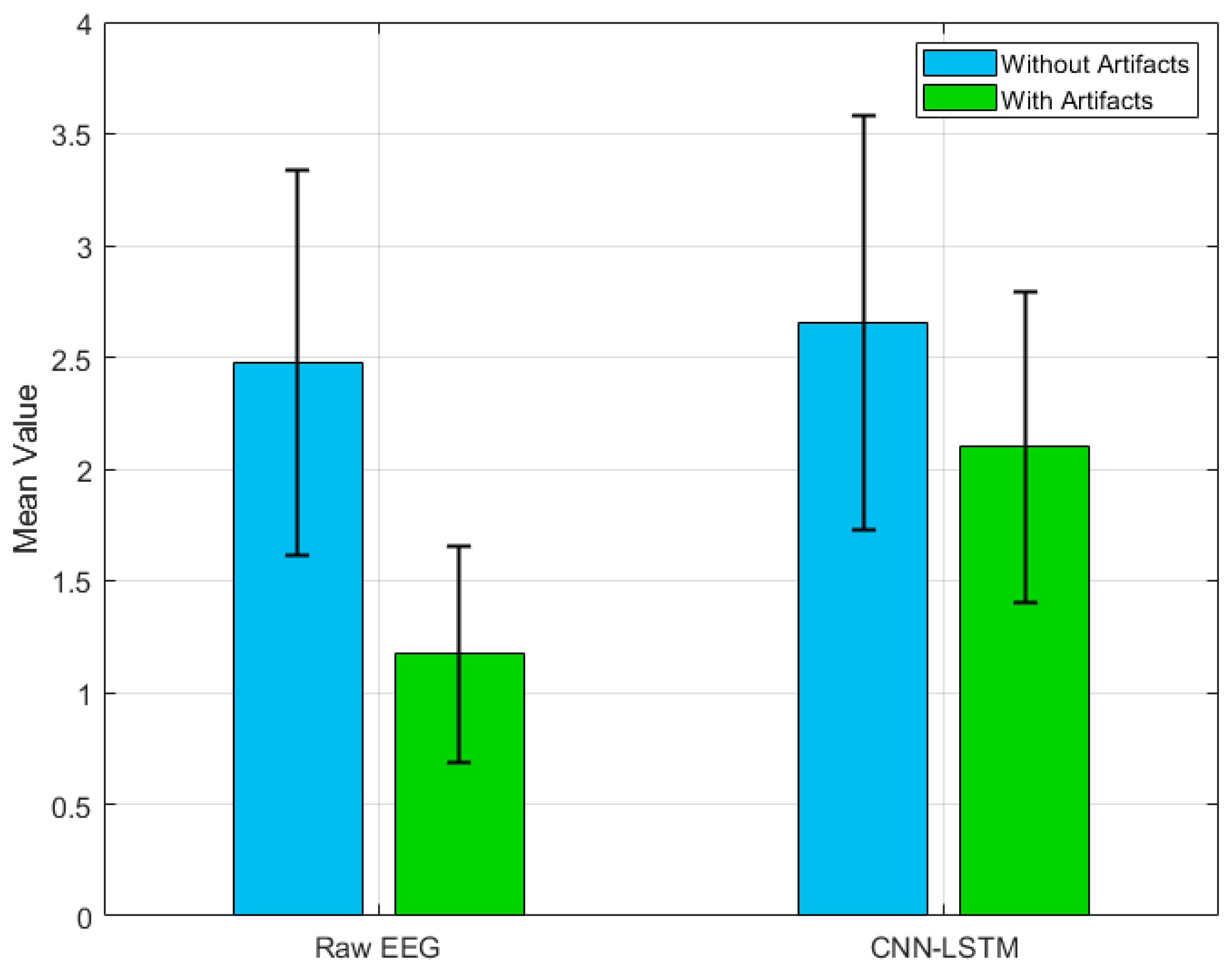
. Figure 13 presents the comparison of the average SNR_SSVEP between the raw EEG and the CNN-LSTM method for one-second EEG signal windows containing jaw-clenching artifacts and artifact-free segments.

It is particularly noteworthy that the CNN-LSTM method applied to signals containing artifacts (average SNR: 2.098) achieves results comparable to those of raw EEG signals without artifacts (average SNR: 2.475; p = 0.028). Another important observation is that, for artifact-free EEG signals, the SNR values remain comparable—the CNN-LSTM processing method does not introduce significant changes compared to the raw signal (raw EEG: 2.475 vs. CNN-LSTM: 2.653; p = 0.34). This indicates that applying the CNN-LSTM method effectively reduces artifact influence to levels typical of interference-free signals while preserving their original structure. In other words, this method accurately reconstructs the actual amplitudes of EEG signals.

6.5. Advantages and Disadvantages of Particular Artifact-Removal Methods

Each artifact removal method has its own advantages and disadvantages. Linear regression is notable for its simplicity of implementation, low computational requirements, and very high processing speed, making it ideal for real-time applications. However, its effectiveness is limited to simple, linear interferences and requires reference signals, which restricts its versatility. ICA decomposes the EEG signal into independent components, effectively separating artifacts without the need for artifact indicator signals. Nevertheless, this method is time-consuming and requires expertise in identifying artifact components, which limits its automation. CNN-LSTM networks represent one of the most advanced approaches, offering high effectiveness in removing complex and nonlinear artifacts, as well as full automation once the model is trained. However, such hybrid networks require large training datasets, substantial computational resources, and time-consuming training processes. Once trained, they operate very quickly, making them well-suited for processing large datasets. In summary, linear regression is the most efficient in terms of speed and simplicity; ICA provides a balance between adaptability and automation; and CNN-LSTM architectures offer superior performance and full automation, albeit at the cost of increased computational demands and data requirements. The choice of method depends on the problem’s specifics, available resources, and requirements for speed and automation.

It should be noted that all methods considered by us use data from additional EMG channels; therefore, they cannot be used with standard EEG hardware nor directly applied to existing EEG data.

6.6. Example of EEG Signal Cleaning for Various Muscle Artifacts

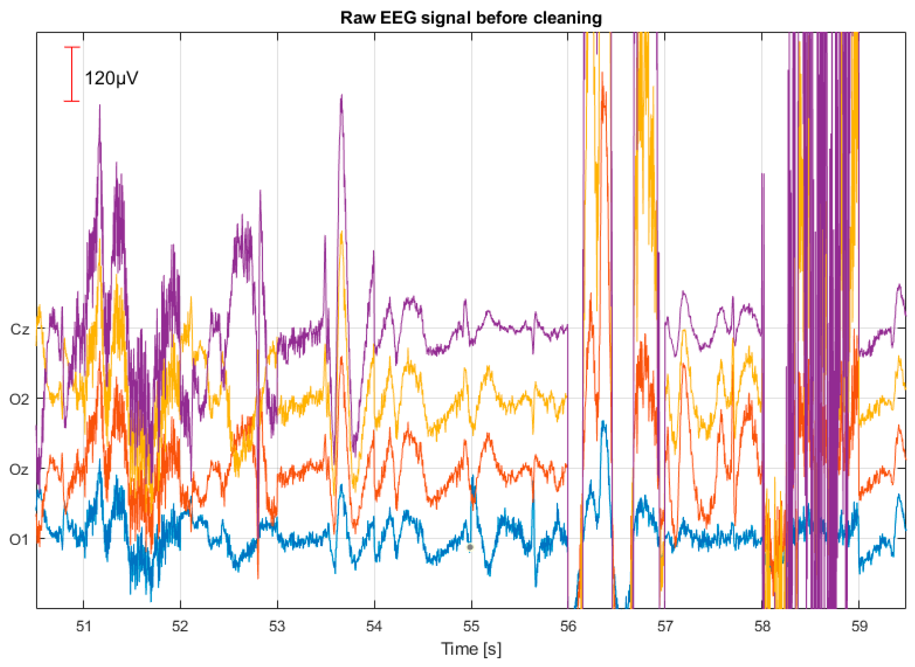
To evaluate how well the proposed method handles more complex EEG signals containing multiple, diverse artifacts, additional experiments were conducted. The EEG was recorded while participants were free to perform any muscle artifacts—or combinations thereof—over a one-minute period. Users combined artifacts such as neck muscle tension, jaw clenching, tongue movements, intense jaw clenching, cheek tension, eye movements, forehead wrinkling, and many others. This generated a mix of artifacts from which it was impossible to isolate a single source of interference. Participants were also asked to perform the artifacts with maximum intensity, posing a significant challenge for the artifact removal algorithm. 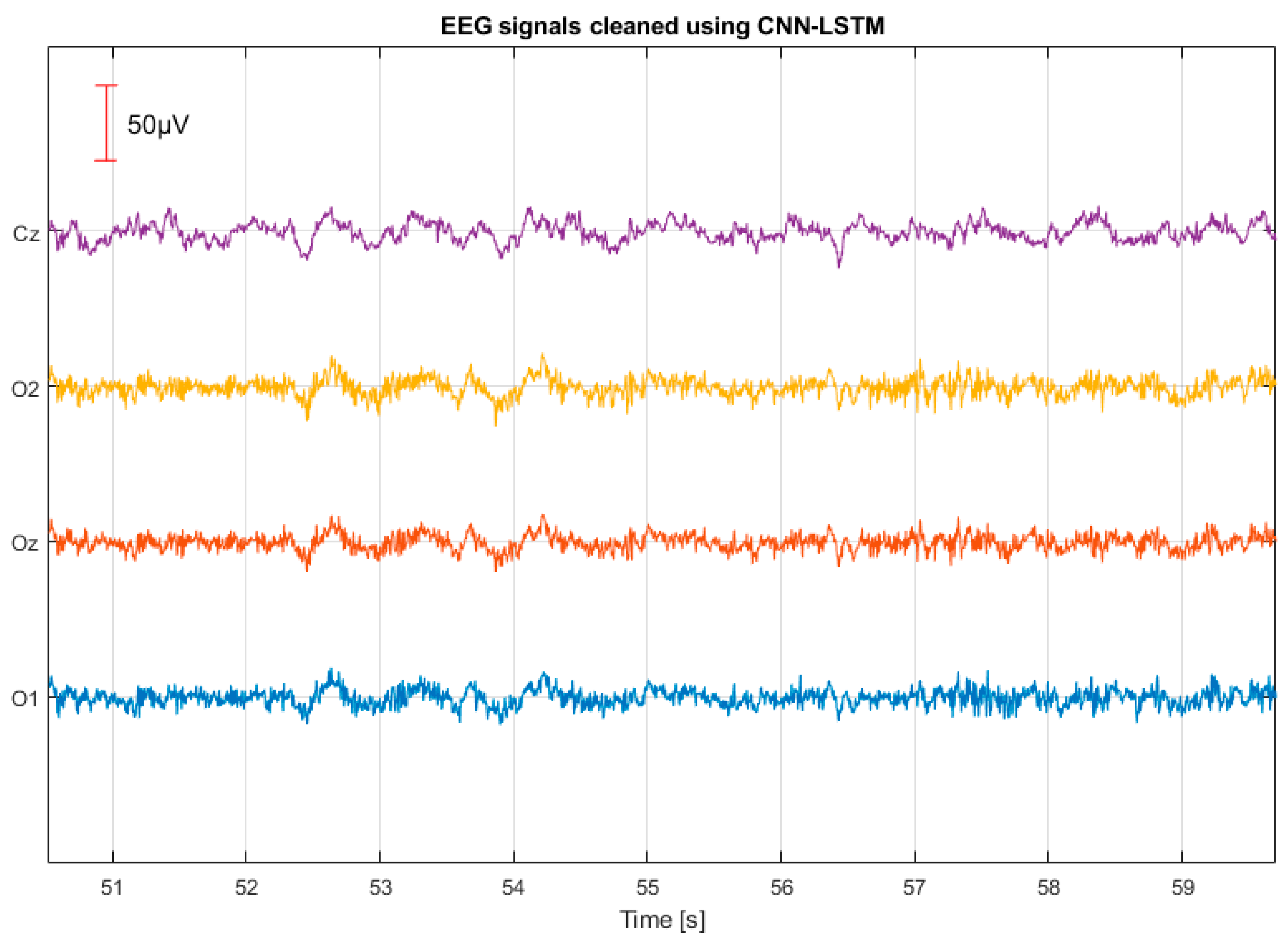Figure 14 shows four EEG channels recorded while one participant was performing these artifacts, and Figure 15 presents the corresponding EEG signals after cleaning with CNN-LSTM method. Both figures are presented on the same amplitude scale. It can be observed that the CNN-LSTM performed remarkably well in eliminating artifacts, even though the algorithm was trained solely on one type of artifact—jaw clenching. The amplitude of the artifacts was significantly reduced. This challenging scenario is particularly relevant to EEG signal analysis in epileptic seizures. These results indicate that the proposed algorithm and method have substantial potential for practical applications.

In the experiment involving “various muscle artifacts”, no visual stimulation (SSVEP) was used, which means the EEG signal lacked evoked potentials that could serve as a reference for evaluating the effectiveness of artifact removal. Simultaneously performing a wide range of artifacts (e.g., eye movements, jaw clenching, neck tension, and facial grimacing) while maintaining steady visual focus on a stimulator is extremely difficult and practically unfeasible. For this reason, only visual inspection was applied, with the same amplitude scale maintained before and after artifact removal, allowing for a qualitative comparison of signal distortion levels. The observed reduction in amplitude and the restoration of characteristic EEG waveforms suggest that the model effectively removes even complex artifacts, despite being trained solely on jaw clenching data. It is worth emphasizing that the data used to train the model underwent extensive augmentation, characterized by high variability. During the generation of synthetic data, many parameters—such as amplitude, temporal structure, and frequency spectrum—were randomly modified. As a result, the training set was significantly more diverse than real-world examples of muscle artifacts originating solely from jaw clenching. Moreover, since muscle artifacts typically have a broad frequency spectrum and irregular characteristics, the model may have learned general features of noise—independent of its source or amplitude. As a result, its behavior may resemble regression, where the model learns the relationship between contaminated and clean signals. This enables the effective removal of previously unseen artifact types—without the need for domain adaptation or transfer learning.

6.7. Practical Applicability of the Proposed CNN-LSTM Algorithm

A key practical consideration is the capability for real-time application; thus, the method’s suitability in this context was evaluated. An analysis was conducted to determine whether the proposed EEG signal denoising method is appropriate for real-time applications, particularly beneficial for brain–computer interface systems. All computations and software implementations were carried out using Python (version 3.9.18) and the TensorFlow library (version 2.10.1). The experiments were performed on a computer equipped with 32 GB of RAM, a Gigabyte GeForce GTX 1660 Ti OC graphics card with 6 GB GDDR6 memory, and an Intel Core i7-9750H CPU running at 2.60 GHz under Windows 10 (64-bit). Results showed that denoising four EEG channels, each with a duration of one second, using the proposed CNN-LSTM-based model took an average inference time of 78 ms. However, the method was developed primarily for the offline processing of entire EEG sessions, leveraging high-performance computing resources. Therefore, no specific optimization for low-power or embedded deployment was performed, as the focus was on maximizing artifact reconstruction quality rather than minimizing computational complexity.

Our research confirms the effectiveness of the proposed method for electrodes O1, O2, and Oz, enabling its use in BCI systems. During the study, we also recorded signals from the Cz channel, which does not contain SSVEP signals. Visual analysis demonstrated that artifacts were effectively removed from this channel as well. Crucially, the signal remained unchanged in regions without artifacts, thus preserving the original EEG structure. We are therefore confident that our method can also be effectively applied to denoising signals from other EEG channels. This capability would extend its practical application to other EEG signal analysis domains, including epilepsy diagnosis, evoked potential analysis, and various clinical and research applications.

6.8. Other Methods Considered for Artifact Removal

During the initial stage of our study, we also considered the use of other commonly applied EEG artifact removal methods, such as adaptive filters—least mean squares (LMS) [26] and recursive least squares (RLS) [27]—as well as artifact subspace reconstruction (ASR) [15].

Adaptive filters such as LMS and RLS are classical approaches used to remove artifacts based on artifact indicator channels—in our case, additional EMG channels. Their main advantage is the ability to dynamically adjust filtering parameters in real time, which theoretically allows for the effective suppression of artifacts with minimal interference to the EEG signal. In our experiments, both LMS and RLS methods enabled a partial reduction of muscle-related artifacts. However, the performance of these filters was highly sensitive to the selection of adaptation parameters—such as the step size in LMS or the forgetting factor in RLS. In many cases, these parameters proved to be very sensitive: overly aggressive settings led to an excessive attenuation of relevant EEG components, while overly lenient settings failed to sufficiently remove the artifacts. Notably, the visual inspection of the EEG signals processed using these filters revealed that in many cases, the filters substantially altered the signal structure—not only in the artifact-contaminated segments but also in those that were potentially clean.

In contrast, ASR is a statistical method that detects and suppresses short-term, atypical deviations from a reference EEG template, treating them as potential artifacts. It can operate in both data rejection and reconstruction modes, making it theoretically comparable to methods that aim to restore the original signal. Nevertheless, we decided not to include ASR in the comparative analysis for several reasons. First, ASR does not utilize direct information about the sources of muscle artifacts. Its operation is based on a statistical model of “clean” EEG and component variance analysis, without the ability to explicitly identify and separate muscle activity as an independent source. This contradicts our core assumption that effective EEG signal reconstruction should, as far as possible, leverage information from EMG channels. Moreover, we conducted tests using ASR on our dataset. As with the adaptive filters, the visual assessment of the EEG signals processed with ASR showed significant signal modifications, particularly in segments with artifacts. We observed waveform smoothing, amplitude changes, and waveform distortions, all of which could negatively affect subsequent analyses. Furthermore, ASR’s effectiveness was clearly subject-dependent, and even within the same recording session, there were instances where some artifacts were either insufficiently removed or removed too aggressively, resulting in undesirable signal distortions. For these reasons, despite ASR’s advantages in general EEG denoising applications, it was not included in our comparative analysis, which focused on reconstructing EEG signals contaminated with EMG artifacts while preserving their natural structure.

6.9. Further Work

Further research should involve recording data that include other types of artifacts while simultaneously presenting stimuli that elicit SSVEP responses. This may be challenging, as interference from EMG artifacts—such as blinking or eye movements—can make it difficult to maintain focus on the flickering visual stimulus and thus prevent SSVEP generation. In future work, it may also be beneficial to present multiple SSVEP stimuli to each participant. This would allow for the use of alternative measures of SSVEP usefulness in brain–computer interfaces, such as classification accuracy. Future studies could focus on further reducing the number of network parameters, for example by applying techniques such as CNN-LSTM distillation.

More detailed analyses are also needed to determine which of the currently used electrodes are truly necessary for recording EMG signals. It may turn out that a smaller number of EMG channels is sufficient, which would simplify and streamline the entire research process. Consideration should also be given to adapting the model for use on embedded and low-power platforms, particularly in real-time BCI applications.

7. Conclusions

Research indicates that adding extra EMG electrodes to monitor muscle artifact sources produces good results in removing such interference. The proposed CNN-LSTM effectively eliminates muscle artifacts while preserving the signal components crucial for analyzing SSVEP. Compared to other methods, such as linear regression or ICA, this approach demonstrates significantly better performance—minimally altering the useful signal and more effectively suppressing interference. Future studies should consider expanding the number of SSVEP stimuli, incorporating additional artifacts, and developing a new, more comprehensive research procedure.