Horizontal Control System for Maglev Ruler Based on Improved Active Disturbance Rejection Controller

Abstract

This paper is centered around the autonomous displacement of the maglev ruler system, with the core objective of optimizing the performance of its horizontal control system. The horizontal positioning precision of the maglev ruler’s mover core plays a crucial role in determining the survey accuracy. Moreover, its horizontal system exhibits distinct nonlinear and strongly coupled characteristics. Initially, a mathematical model is meticulously established based on the principles of magnetic circuits and dynamics. By analyzing the relationship between the Ampere force and the coil current, and constructing the dynamic equations, it is clearly demonstrated that this system belongs to a nonlinear and strongly coupled type with two inputs and two outputs. Subsequently, the active disturbance rejection control algorithm is employed to address the decoupling issue, and a novel differential tracker, SYSTD, is designed. SYSTD is constructed using specific elementary functions. Through rigorous theoretical derivation, its favorable stability is verified. The basis for parameter selection is obtained through phase-plane analysis, and a detailed tuning method is provided. Additionally, a sensor-less control technology is proposed, where survey coils are wound along the horizontal control coils to estimate the position of the mover core. The simulation and experimental results indicate that the improved system showcases excellent performance. In the simulation, the positioning accuracy can reach ±5 μm, while, in the experiment, the control accuracy can achieve ±2 μm. It can effectively realize decoupling control and possesses good dynamic, static characteristics, as well as remarkable robustness. This research paves the way for the practical application of the maglev ruler system in fields such as coordinate survey.

1. Introduction

The linear survey system of a coordinate measuring machine (CMM) is composed of a grating scale, a servo motor, and a linear motion mechanism, enabling the survey of free-form surface components [1,2]. The maglev ruler has the potential to simplify this system, as its mover core (MRC) undertakes the functions of autonomous displacement and displacement survey [1,2]. The MRC of the maglev ruler (MAR) moves in a step-by-step linear fashion with a fixed step size. The microcontroller determines its displacement by recording the number of steps, and the horizontal positioning precision of the MRC directly influences the survey accuracy of the MAR [1,2]. This paper delves into the research on the horizontal displacement system of the MAR. A mathematical model is established based on the principles of magnetic circuits and dynamics, the improved active disturbance rejection control algorithm is utilized to solve the nonlinear and strongly coupled problems of the system, and the sensor-less control technology is adopted to simplify the system structure [1,2]. Active disturbance rejection control (ADRC), particularly effective in handling nonlinear and coupled systems [3,4,5,6,7], is adopted to address the horizontal motion control challenges. Its core mechanism—real-time estimation and compensation of total disturbances via an extended state observer (ESO)—aligns with the requirements of the maglev ruler’s horizontal system.

ADRC has demonstrated success in maglev systems, such as yaw angle control [8] and rotor stabilization [9]. However, its application to horizontal motion control of maglev rulers remains unexplored. The rotor of a maglev turbo machine is subject to various disturbances, and traditional PID control has limitations [10]. The linear active disturbance rejection controller (LADRC) improves upon the shortcomings of PID but still has issues such as overshoot. The improved LADRC suppresses uncertain factors through specific design, facilitating its application in engineering [10]. Conventional tracking differentiators (TDs) face challenges in balancing noise suppression and response speed [11,12,13,14]. To overcome these limitations, a novel TD (SYSTD) is designed, as detailed in Section 5. The fhan-TD with double r improves its performance through innovative design, and its advantages have been verified by simulations and experiments [14]. In the field of electric vehicles, to address the speed-regulation contradiction of permanent-magnet synchronous motors, a study proposed MTD-DADRC [15]. This controller is applied in the speed loop control, which improves the system stability and anti-noise ability and enhances the speed tracking performance of the motor. Compared with the traditional PI controller, it can shorten the shift-speed-regulation time and reduce the shift shock [15]. There is also a study that proposed an active disturbance rejection fractional-order controller (ADRFOC) for time-delay systems to achieve independent control of servo and regulation [16]. Comprising FOC and MESO, its effectiveness was verified through mathematical derivation. The air-floating motion platform experiment shows that its performance outperforms that of typical time-delay ADRC and SIMC-PID controllers [16]. When the MAR system conducts surveys, the MRC moves in a step-by-step manner, resulting in a high-frequency fluctuation of its position feedback signal. Classical TD and MTD cannot meet the response speed requirements when dealing with such fast-changing signals, leading to tracking delays. This will affect the real-time tracking precision of the MRC position, thereby reducing the positioning accuracy of the horizontal control system (HCS) of the MAR system and making it impossible to quickly and accurately obtain the position information of the MRC. Furthermore, in the MAR system, obtaining accurate position and speed information is of utmost importance. In the field of motor control, relevant technologies can offer valuable references [17,18,19,20,21]. For example, in the research of permanent-magnet linear synchronous motors (PMLSMs), the method of combining an ADRC speed controller and an AFO position estimator can improve the position estimation accuracy and can be applied in the MAR system to enhance the position estimation accuracy of the MRC [19]. The ADRC-enhanced sensorless vector control method of permanent-magnet synchronous motors (PMSMs) has strong anti-interference capabilities and is helpful for improving the anti-interference ability of the MAR system [20]. A new hybrid algorithm for switched reluctance motors (SRMs) can accurately estimate the motor state. When applied to the MAR system, it can improve its survey accuracy [21].

Previous studies have laid the foundation for the maglev ruler: The literature of [1] proposed the structural design and magnetic circuit analysis, while the literature of [2] focused on the suspension control system to stabilize the mover core vertically. However, neither addressed the horizontal motion control of the mover core, which is critical for precise positioning in coordinate measurement. In the existing literature, the horizontal control of the maglev ruler’s mover core has not been systematically investigated. The proposed method addresses the inherent nonlinearity and strong coupling characteristics of the horizontal system, overcoming the limitations of conventional linear control strategies such as PID. The contributions of this study include (1) an optimized winding configuration for horizontal control coils and analysis of their operational principles; (2) a novel active disturbance rejection control (ADRC) framework based on SYSTD, achieving decoupling control; and (3) a sensor-less position estimation technology that enables high-precision localization through measurement coils.

This paper conducts in-depth research on the autonomous displacement of the MAR system. Besides the abstract and introduction, it consists of seven parts. The second part focuses on establishing the mathematical model of the horizontal system and analyzing the relationship between the Ampere force and the coil current. The third part constructs the dynamic model to describe the movement of the MRC. The fourth part uses ADRC for decoupling. The fifth part designs the improved tracking differentiator SYSTD. The sixth part elaborates on the ESO, NLSEF, and disturbance compensation of ADRC. The seventh part provides the system parameter tuning method and conducts simulations. The eighth part summarizes the research, verifies the system performance, demonstrates its high positioning accuracy, and lays a solid foundation for subsequent research.

2. Mathematical Model of the Horizontal System

2.1. Modeling of Horizontal Thrust-Current Dynamics

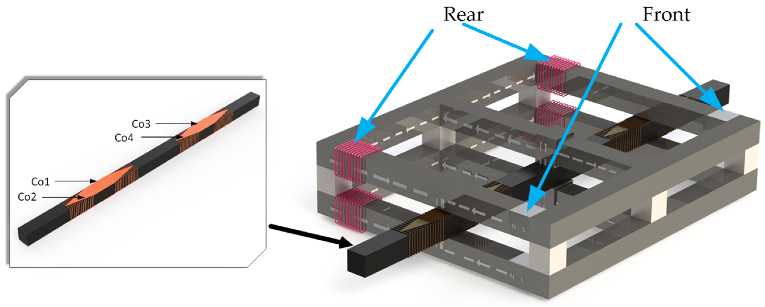
The “moving armature” method is adopted, with the horizontal control coils wound around the MRC [2]. The Ampere force generated in the horizontal direction by the energized horizontal control coils in the air-gap magnetic field drives the MRC to move horizontally. The winding configuration of the horizontal control coils is depicted in Figure 1.

The MAR system is equipped with six stator yokes in the Y-direction. The air-gap magnetic fields between the two sets of stator yokes on both sides and the MRC share the same direction. However, the air-gap magnetic field between the middle stator yoke and the MRC has an opposite direction to that of the side stator yokes. If a coil is wound around the entire MRC along its Y-axis, the Ampere forces acting on the MRC in the three magnetic fields will not be in the same direction. The Ampere forces at the two-side force-application points of the MRC are in the same direction, which is contrary to the Ampere force at the middle force-application point. Since the MRC is driven by the Ampere forces on both sides, the Ampere force in the middle interferes with the movement of the MRC. Consequently, no coil is wound in the middle part of the MRC. Instead, four coils, Co1, Co2, Co3, and Co4, are wound on both sides of the MRC. As illustrated in Figure 1, Co1 and Co2 are fastened to one side of the MRC from the front and rear, while Co3 and Co4 are attached to the other side of the MRC from the front and rear. This setup ensures that the wires of the horizontal control coils in the air-gap magnetic field are perpendicular to the Y-direction. In this paper, the permanent magnet of the MAR system is designated as the front side of the system, and the suspension control coils are considered the rear side. After energization, Co1 can generate a forward-driving force, propelling one end of the MRC forward. Similarly, Co3 can drive the other end of the MRC forward. Co2 and Co4 generate backward-driving forces to move the MRC backward. As there are no wires in the air-gap magnetic field at the middle of the MRC, no reverse interference force is generated. 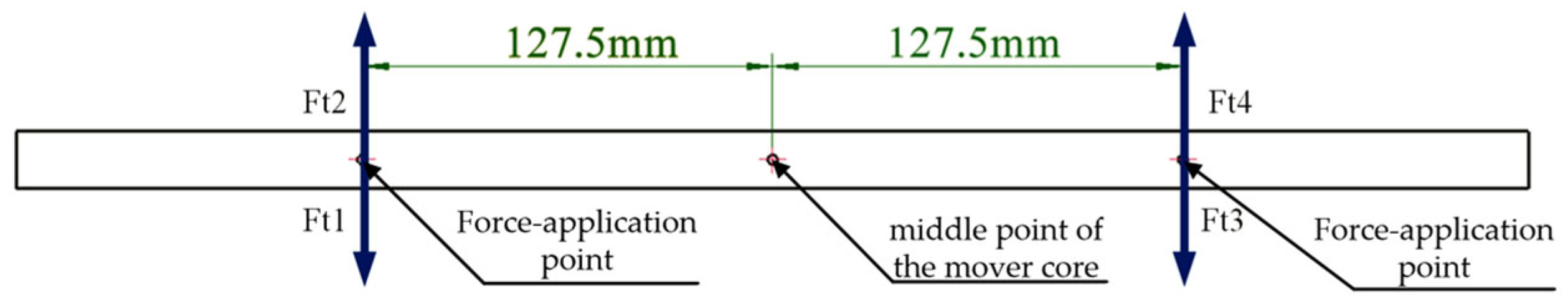Figure 2 presents the schematic diagram of the horizontal driving force.

In the figure, F_t1 represents the Ampere force generated by the energization of coil Co1, F_t2 is the Ampere force generated by the energization of coil Co2, F_t3 is the Ampere force generated by the energization of coil Co3, and F_t4 is the Ampere force generated by the energization of coil Co4. Therefore, the thrust on the right-hand side of the MRC is as follows:

$$F_{rt}=F_{t1}-F_{t2}$$

(1)

Based on the Ampere force calculation formula [2], the formula for calculating the right-hand side thrust F_rt is as follows:

$$F_{rt}=n{B}_{r}L{i}_{cr}$$

(2)

In this formula, n is the sum of the turns of the right-front horizontal control coil and the right-rear horizontal control coil. Each group of coils has 15 turns, amounting to a total of 30 turns. B_r represents the sum of the right-hand side air-gap magnetic fields. L is the length of a single-turn horizontal control coil in the air-gap magnetic field. i_cr is the current of the horizontal control coils on the right-hand side of the MRC, which is composed of the current i_c1 of the right-front horizontal control coil Co1 and the current i_c2 of the right-rear horizontal control coil Co2. i_c1 and i_c2 flow in opposite directions. When observing the two horizontal control coils Co1 and Co2 on the right-hand side from the front side of the MAR system, if the current i_c1 in coil Co1 flows counter-clockwise, it is considered positive, ensuring that the horizontal control coil Co1 generates a forward thrust F_t1. If the current i_c2 in coil Co2 flows clockwise, it is negative, ensuring that the horizontal control coil Co2 generates a backward thrust F_t2. Then, the following is true:

$$\left\{\begin{array}{l}{i}_{cr}=i_{c1} i_{c1}\ge 0, i_{c2}=0 \hfill \\ i_{cr}=i_{c2} i_{c2}<0, i_{c1}=0\hfill \end{array}\right.$$

(3)

When the MRC accelerates forward, i_c2 is zero, and at this moment, i_cr = i_c1. When the MRC accelerates backward, i_c1 is zero, and i_cr = i_c2. Similarly, the thrust on the left-hand side of the MRC is as follows:

$$F_{lt}=F_{t3}-F_{t4}$$

(4)

According to the Ampere force calculation formula [2], the formula for calculating the left-hand side thrust F_lt is as follows:

$$F_{lt}=n{B}_{l}L{i}_{cl}$$

(5)

In this formula, n is the sum of the turns of the left-front horizontal control coil and the left-rear horizontal control coil, with a total of 30 turns. B_l is the sum of the left-hand side air-gap magnetic fields. L is the length of a single-turn horizontal control coil in the air-gap magnetic field. i_cl is the current of the horizontal control coils on the left-hand side of the MRC, composed of the current i_c3 of the left-front horizontal control coil Co3 and the current i_c4 of the left-rear horizontal control coil Co4. i_c3 and i_c4 flow in opposite directions. When looking at the two horizontal control coils Co3 and Co4 on the left-hand side from the front side of the MAR system, if the current i_c3 in coil Co3 flows counter-clockwise, it is positive, enabling the horizontal control coil Co3 to generate a forward thrust. If the current i_c4 in coil Co4 flows clockwise, it is negative, allowing the horizontal control coil Co4 to generate a backward thrust. Then, the following is true:

$$\left\{\begin{array}{l}{i}_{cl}=i_{c3} i_{c3}\ge 0, i_{c4}=0 \hfill \\ i_{cl}=i_{c4} i_{c4}<0, i_{c3}=0\hfill \end{array}\right.$$

(6)

When the MRC accelerates forward, i_c4 is zero, and i_cl = i_c3. When the MRC accelerates backward, i_c3 is zero, and i_cl = i_c4. As can be seen from Figure 1, the horizontal control coils on the left-hand side and the right-hand side are positioned far apart, and the magnetic field interference between them can be neglected. Thus, the thrusts at both ends of the MRC are not coupled.

2.2. The Relationship Between the Horizontal Thrust and the Current of the Horizontal Control Coil

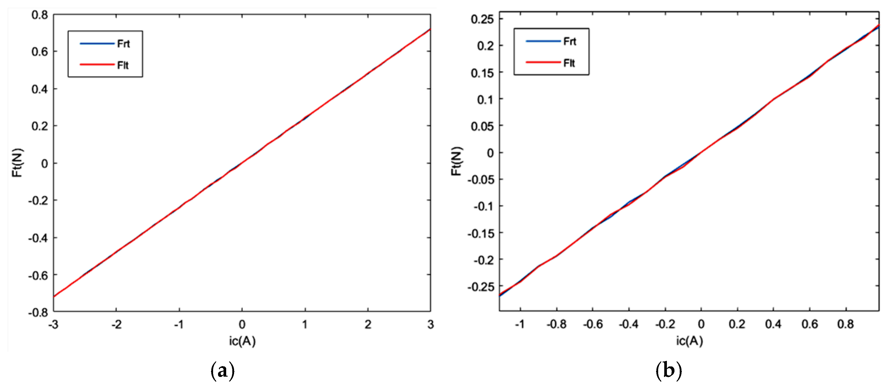
Thrust and the Current of the Horizontal Control Coil Force sensors are respectively fixed on the front and rear sides of the MRC to measure a set of horizontal thrust values when the current of the horizontal control coils ranges from −2A to +2A. The relationship between the horizontal thrust and the current of the horizontal control coil is then plotted, as shown in Figure 3. In this paper, the forward thrust is defined as positive.

In Figure 3, F_rt represents the thrust on the right-hand side of the MRC, and F_lt represents the thrust on the left-hand side. It can be observed from Figure 3a that the current of the horizontal control coils on both sides of the MRC is proportional to the thrust generated by the coils. However, due to the parallel installation and close proximity of Co1 and Co2, as well as Co3 and Co4, the mutual inductance coefficient between Co1 and Co2 is nearly 1, and the same is true for Co3 and Co4. As a result, when i_cr changes from positive to negative, that is, during the process of i_c1 decreasing to zero, there is mutual inductance in Co2, and this mutual inductance does not disappear when i_c1 reaches zero. During the process of i_c2 gradually increasing, although the mutual inductance decreases, it still has an impact on the thrust. From Figure 3b, it can be seen that near the origin of the coordinate system, the thrust exhibits fluctuations. Given that the fluctuation range is very small, it can be disregarded.

3. Dynamic Model of the Horizontal System

Based on the thrust analysis in Figure 2, the MRC has two degrees of freedom in the horizontal system: (1) it can move vertically in the Y-direction; (2) it can rotate around the Z-axis with the center of mass of the MRC as the center of rotation, denoted as ψ_z. In this paper, Newton’s second law of motion is utilized to describe the vertical motion of the MRC, and the torque equation is employed to describe its rotational motion [2].

$$F_y=m\cdot {\displaystyle \frac{{\partial }^2{y}_b}{\partial t^2}}$$

(7)

$$M_{\beta }=J_{\beta }\cdot {\displaystyle \frac{{\partial }^2{\psi }_z}{\partial t^2}}$$

(8)

In Equation (7), F_y represents the sum of all forces acting on the MRC in the Y-direction, m is the mass of the MRC, and y_b is the displacement of the center of mass of the MRC in the Y-direction. In Equation (8), M_β is the torque of the resultant force F, J_β is the moment of inertia, and ψ_z is the rotation angle. The position of the center of mass, the force-application points of the horizontal thrusts at the left and right ends of the MRC, and the length of the force arm are marked in Figure 2.

$$J_{\beta }=m_h{r}^2$$

(9)

In Equation (9), m_h is the mass from the center of mass of the MRC to the end, and r is the distance from the center of mass to the force-application point of the horizontal thrust. From this, J_β = 1.49 × 10⁻² kg·m² can be calculated. Ignoring other disturbances such as base vibration and suspension force, the sum of all forces F_y on the MRC in the Y-direction is as follows:

$$F_y=F_{lt}+F_{rt}$$

(10)

From the dimensions indicated in Figure 2, the torque equation around the Y-axis is as follows:

$$M_{\beta }=-0.1275F_{lt}+0.1275F_{rt}$$

(11)

According to Equation (8), the following can be obtained:

$$-0.1275F_{lt}+0.1275F_{rt}=J_{\beta }\cdot {\displaystyle \frac{{\partial }^2{\psi }_z}{\partial t^2}}$$

(12)

From Equations (7) and (10), we obtain the following:

$$F_{lt}+F_{rt}=m\cdot {\displaystyle \frac{{\partial }^2{y}_b}{\partial t^2}}$$

(13)

Thus, the rigid-body dynamic equation of the MRC horizontal system is derived as follows:

$$\left[\begin{array}{cc}1& 1\\ -0.1275& 0.1275\end{array}\right]\cdot \left[\begin{array}{c}{F}_{lt}\\ F_{rt}\end{array}\right]=\left[\begin{array}{cc}1.83& 0\\ 0& 0.0273\end{array}\right]\left[\begin{array}{c}{\displaystyle \frac{{\partial }^2{y}_b}{\partial t^2}}\\ {\displaystyle \frac{{\partial }^2{\psi }_z}{\partial t^2}}\end{array}\right]$$

(14)

The MRC is solely affected by the horizontal thrust in the horizontal direction. According to Newton’s second law, F_lt and F_rt are related to the left-hand side horizontal displacement y_bl and the right-hand side horizontal displacement y_br of the MRC, and they are in the [y_bl, y_br] coordinate system with the horizontal displacement as the research point. However, Equation (14) is in the [y_b, ψ_z] coordinate system with the center of mass as the research point. Therefore, a coordinate transformation is required to convert the horizontal displacement coordinate system to the center-of-mass coordinate system.

As can be seen from Figure 2, when the MRC rotates around the Z-axis, there are the following relationships between y_bl, y_br, the displacement of the center of mass y_b and the rotation angle ψ_z:

$$y_{bl}=y_b-0.1275\times \tan {\psi }_z$$

(15)

$$y_{br}=y_b+0.1275\times \tan {\psi }_z$$

(16)

Since the horizontal displacement is extremely small, the rotation angle ψ_z is also very small, so tan ψ_z ≈ ψ_z. Therefore, Equations (4)–(15) and (4)–(16) can be written as follows:

$$\left[\begin{array}{c}{y}_{bl}\\ y_{br}\end{array}\right]=\left[\begin{array}{cc}1& -0.1275\\ 1& 0.1275\end{array}\right]\left[\begin{array}{c}{y}_b\\ {\psi }_z\end{array}\right]$$

(17)

The above formula can be used to transform the horizontal displacement coordinate system into the center-of-mass coordinate system.

Substitute Equations (2) and (5) into Equation (14), and, after rearrangement, the horizontal system analysis model of the MAR system can be obtained:

$$\left[\begin{array}{cc}0.21& 0.21\\ -0.0268& 0.0268\end{array}\right]\cdot \left[\begin{array}{c}{i}_{cl}\\ i_{cr}\end{array}\right]=\left[\begin{array}{cc}1.83& 0\\ 0& 0.0273\end{array}\right]\left[\begin{array}{c}{\displaystyle \frac{{\partial }^2{y}_b}{\partial t^2}}\\ {\displaystyle \frac{{\partial }^2{\psi }_z}{\partial t^2}}\end{array}\right]$$

(18)

The boundary conditions for Equation (18) are defined by the physical constraints of the maglev ruler:

Initial states: y_b(0) = 0, ψ_z(0) = 0;

Motion range limits: y_b ≤ 1.2 mm, ψ_z ≤ 0.01 rad to avoid mechanical interference;

Actuator saturation: i_cr ≤ 2 A, i_cl ≤ 2 A.

These constraints reflect the system’s nonlinearity and coupling, which cannot be handled by linear controllers like PID.

It can be seen from Equation (18) that the horizontal system of the MAR system is a nonlinear system with a double-input and double-output structure. Moreover, there is a strong coupling in the system. Conventional linear control methods cannot effectively control the system. The ADRC method is more suitable for the horizontal system of the magnetic levitation ruler system.

4. HCS Based on Active Disturbance Rejection

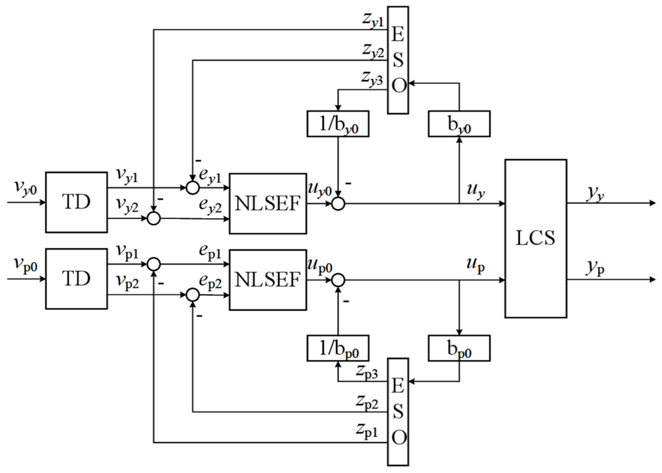
The HCS of the MAR is a coupled system. In view of this, this paper utilizes the characteristics of the ADRC, a system that has low requirements for modeling accuracy and can effectively compensate for comprehensive disturbances, to solve the decoupling problem in the horizontal system of the MAR. The ADRC regards the coupling between various degrees of freedom (y_b and ψ_z) as disturbances, observes them through an ESO, and compensates for their combined effects (i.e., the total disturbance of the system), thereby achieving decoupling control. Essentially, this compensation is a means of anti-disturbance. This control method has low requirements for the model and is easy to implement, which can effectively solve the problems of decoupling and disturbance suppression in horizontal control.

The ADRC controller of the HCS is shown in Figure 4. It mainly consists of a tracking differentiator (TD), an extended state observer (ESO), and a nonlinear state error feedback control law (NLSEF).

5. Improved Tracking Differentiator (SYSTD)

When the MAR system measures, the MRC adopts a step-by-step motion mode with a fixed step size, resulting in a high-frequency fluctuation of its position feedback signal. High-quality position feedback signals contribute to improving the positioning accuracy of the HCS of the MAR system. Although classical tracking differentiators can reduce differential noise, do not require the derivation of a mathematical model, and are convenient to use, they also have problems such as complex and diverse forms, insufficient stability, large phase delay, or amplitude attenuation. The above problems can be solved by improving the structure of TD and enhancing its performance.

5.1. Design and Stability Judgment of SYSTD

The key to constructing a new type of tracking differentiator lies in designing an acceleration function with both linear and nonlinear characteristics. Since sign functions and piece-wise functions can increase switching noise, they are not suitable for application. Therefore, this paper employs elementary functions, which are defined as follows:

$$sys(x,a_4,a_5)={\displaystyle \frac{x}{\sqrt{a_4+a_5{x}^2}}}$$

(19)

where a₄ > 0, a₅ > 0, a₄ ∈ R, a₅ ∈ R. The following can be deduced:

$$\left\{\begin{array}{l}\underset{x\to +\infty }{\lim }sys={\displaystyle \frac{1}{\sqrt{a_5}}},\underset{x\to -\infty }{\lim }sys={\displaystyle \frac{-1}{\sqrt{a_5}}}\hfill \\ sys(x)+sys(-x)=0\hfill \end{array}\right.$$

(20)

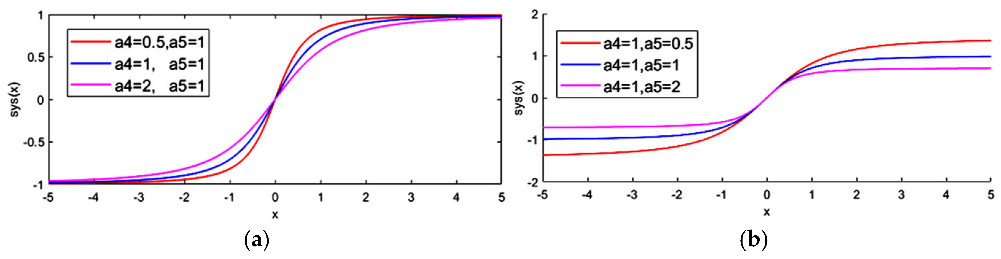
It can be seen that sys(x) is a smooth and continuous odd function passing through the first and third quadrants, and it is bounded.

Its basic characteristics are shown in Figure 5. As can be seen from Figure 5a, the parameter a₄ can adjust the curve change rate. The smaller the value of a₄, the greater the curve change rate. When x > 1 or x < −1, the function curve gradually approaches saturation; when −1 < x < 1, the function is approximately linearly changing, and, the smaller the value of a₄, the larger the slope. It can also be seen from Figure 5a that the parameter a₅ can adjust the amplitude of the curve, that is, the saturation boundary. This indicates that the TD based on the sys(x) function has good tracking and differential characteristics, and the sys(x) function requires fewer parameters to be adjusted. Therefore, the following second-order system S₀ is constructed:

$$\left\{\begin{array}{l}{\dot{z}}_1(t)=z_2(t)\hfill \\ {\dot{z}}_2(t)=-sys(z_1(t),a_{41},a_{51})-sys(z_2(t),a_{42},a_{52})\hfill \end{array}\right.$$

(21)

To design SYSTD, Lemma 1 needs to be introduced first.

Figure 5. (a) The curve of the function sys(x) when the parameter a₄ changes and the parameter a₅ remains unchanged. (b) The curve of the function sys(x) when the parameter a₅ changes and the parameter a₄ remains unchanged.

Figure 5. (a) The curve of the function sys(x) when the parameter a₄ changes and the parameter a₅ remains unchanged. (b) The curve of the function sys(x) when the parameter a₅ changes and the parameter a₄ remains unchanged.

Lemma 1

[22]. For a time-invariant system S:

$$\left\{\begin{array}{l}{\dot{x}}_1=x_2\hfill \\ {\dot{x}}_2=f(x_1,x_2)\hfill \end{array}\right.\hspace{1em}{x}_1,x_2\in D\subset R^2$$

(22)

If in the real domain R²:

(1) There exists a positive-definite function (or negative-definite function) V(x) that increases infinitely;

(2) In the entire phase space, the total derivative of V(x) along the solution of system S with respect to time t is always negative (or always positive);

(3) The set of points that satisfy only contains the origin.

Then the zero-solution of the system is globally asymptotically stable.

Theorem 1.

When the parameters a₄₁, a₅₁, a₄₂, and a₅₂ are all greater than zero, the system S₀ satisfies the Lyapunov global asymptotic stability condition:

$$\begin{array}{l}\underset{t\to \infty }{\lim }{z}_1(t)=0\\ \underset{t\to \infty }{\lim }{z}_2(t)=0\end{array}$$

(23)

Proof. 

First, construct the Lyapunov function as follows:

$$V(z_1,z_2)={\displaystyle {\int }_0^{z_1}sys(\xi ,a_4,a_5)d\xi +\frac{1}{2}{z}_2^2}$$

(24)

when a₄ > 0 and a₅ > 0, because the function sys(ξ, a₄, a₅) is an odd function and is monotonically increasing in the first and third quadrants, the variable ξ and the function sys(ξ, a₄, a₅) always have the same sign. Therefore, the following is true:

$${\displaystyle {\int }_0^{z_1}sys(\xi ,a_4,a_5)d\xi \ge 0}$$

(25)

Equation (25) holds with the equal sign only when z₁ = 0. When z₁ ≠ 0, according to Equations (24) and (25), V(z₁,z₂) > 0 always holds. Therefore, there exists a positive-definite function V(z₁,z₂) that increases infinitely.

Secondly, take the derivative of the function V(z₁,z₂) with respect to time t:

$$\dot{V}(z_1,z_2)=sys(z_1,a_{41},a_{51})\cdot z_2+z_2{\dot{z}}_2=-z_2\cdot sys(z_2,a_{42},a_{52})\le 0$$

(26)

It can be seen from Equation (26) that the equal sign holds only when z₂ = 0. When z₂ ≠ 0, the function always holds. Therefore, in the entire phase space, the total derivative of V(z₁,z₂) along the solution of system S₀ with respect to time t is always negative.

Thirdly, it is known that the equal sign of Equation (26) holds only when z₂ = 0. At this time, this occurs only when z₁ = 0, ${\dot{\mathrm{z}}}_2=0$. Therefore, the set of points that satisfy $\dot{V}(z_1,z_2)=0$ only contains the origin (0, 0).

Finally,

When $\left|z_1\right|\to +\infty$, ${\displaystyle {\int }_0^{z_1}sys(\xi ,a_{41},a_{51})}d\xi \to +\infty$;

When $\left|z_2\right|\to +\infty$, ${\displaystyle \frac{1}{2}}{z}_2^2\to +\infty$.

Therefore, V(z₁,z₂) tends to positive infinity in the real domain R².

It can be seen from Lemma 1 that the zero-solution of system S₀ is globally asymptotically stable. The proof is completed. □

Next, this paper designs TD based on the function sys(). Lemma 2 needs to be introduced first.

Lemma 2 

[22]. In the sense of Filippov, if the second-order differential equation is as follows:

$$\left\{\begin{array}{l}{\dot{z}}_1(t)=z_2(t)\hfill \\ {\dot{z}}_2(t)=f(z_1(t),z_2(t))\hfill \end{array}\right.$$

(27)

Additionally, if it has all solutions bounded and satisfies the following:

$$\left\{\begin{array}{l}\underset{t\to \infty }{\lim }{z}_1(t)=0\hfill \\ \underset{t\to \infty }{\lim }{z}_2(t)=0\hfill \end{array}\right.$$

(28)

Then, for any bounded measurable signal r(t) (t ∈ [0, +∞]) and time T(T > 0), there is a differential equation S₁:

$$\left\{\begin{array}{l}{\dot{x}}_1(t)=x_2(t)\hfill \\ {\dot{x}}_2(t)=R^{2}f(x_1(t)-r(t),{\displaystyle \frac{x_2(t)}{R}})\hfill \end{array}\right.$$

(29)

The solution component x₁(t) of S₁ satisfies the following:

$$\underset{R\to \infty }{\lim }{\displaystyle {\int }_0^T\left|x_1(t)-r(t)\right|dt=0}$$

(30)

It can be seen from Lemma 2 that, within any finite time T, as R increases, x₁(t) can fully approximate the input signal r(t). Combining this with Equation (21), the system S₂ is constructed as follows:

$$\left\{\begin{array}{l}{\dot{x}}_1=x_2\hfill \\ {\dot{x}}_2=R^2[-sys(x_1-r,a_{41},a_{51})-sys({\displaystyle \frac{x_2}{R}},a_{42},a_{52})]\hfill \end{array}\right.$$

(31)

Theorem 2.

If a₄₁, a₅₁, a₄₂, and a₅₂ are all positive numbers, and the $\dot{r}(t)$ and $\ddot{r}(t)$ of the input signal r(t) (t ∈ [0, +∞]) are bounded, then, for any finite time T > 0, the system S₂ satisfies:

(1) The solutions of system S₂ satisfy the following:

$$\underset{R\to \infty }{\lim }{\displaystyle {\int }_0^T\left|x_1(t)-r(t)\right|dt=0}$$

(32)

Furthermore, x₁(t) converges to r(t), and x₂(t) converges to the generalized derivative of r(t).

(2) System S₂ is a perturbed form of system S₁.

Proof. 

First, because S₂ and S₁ are equivalent in form, it can be seen from Lemma 2 that conclusion (1) holds.

Secondly, let the following be true:

$$\begin{array}{l}\eta =Rt\\ w_1(\eta )=x_1(t)-r(t)\\ w_2(\eta )={\displaystyle \frac{x_2(t)}{R}}\end{array}$$

(33)

Take the derivatives of w₁ and w₂ to obtain the following:

$$\begin{array}{l}{\displaystyle \frac{d{w}_1(\eta )}{dt}}=w_2(\eta )-{\displaystyle \frac{\dot{r}(\frac{\eta }{R})}{R}}\\ {\displaystyle \frac{d{w}_2(\eta )}{dt}}=-sys(w_1(\eta ),a_{41},a_{51})-sys(w_2(\eta ),a_{42},a_{52})\end{array}$$

(34)

When R → ∞, system Equation (34) is equivalent to system S₀. At this time, z₁ and z₂ are not only the solutions of system S₀ but also the solutions of system Equation (33). Therefore, system S₂ is a perturbed form of system S₀ and has global zero-value asymptotic stability. The conclusion (2) holds and the proof is completed. □

System S₂ is SYSTD. Obviously, the dynamic performance of SYSTD is affected by the parameters a₄₁, a₅₁, a₄₂, a₅₂, and R.

5.2. Phase-Plane Analysis of the Tracking Differentiator System

By studying the types of singular points and the characteristics of phase-trajectories in the system phase-plane, the convergence characteristics of the second-order nonlinear time-invariant system can be analyzed, and, thus, the constraint conditions of the parameters can be obtained.

First, perform a Taylor expansion of the function sys(x,a₄,a₅) at the zero point. Its expansion with remainder is as follows:

$$y={\displaystyle \frac{1}{\sqrt{a_4}}}(x-{\displaystyle \frac{a_5*x^3}{2*a_4}}+{\displaystyle \frac{3*a_5^2*x^5}{8*a_4^2}}-{\displaystyle \frac{5*a_5^3*x^7}{16*a_4^3}}+{\displaystyle \frac{35*a_5^4*x^9}{128*a_4^4}}\cdots )+R_n(x)$$

(35)

The absolute-value ratios of the first-order term coefficient to other multi-order term coefficients are ${\displaystyle \frac{2a_4}{a_5}}$, ${\displaystyle \frac{8a_4^2}{3a_5^2}}$, ${\displaystyle \frac{16a_4^3}{5a_5^3}}$, ${\displaystyle \frac{128a_4^4}{35a_5^4}}$, etc. If the linear part of the function sys() is to play a dominant role in the extremely small neighborhood of x = 0 and reduce the chattering of the TD output, it is necessary to set, which can increase the weight of the linear part. Therefore, in the extremely small neighborhood of x = 0, there is the following:

$$sys(x,a_4,a_5)\approx {\displaystyle \frac{x}{\sqrt{a_4}}}$$

(36)

At this time, system S₀ can be approximately expressed as a linear system S₃, which is as follows:

$$\left\{\begin{array}{l}{\dot{z}}_1(t)=z_2(t)\hfill \\ {\dot{z}}_2(t)=-{\displaystyle \frac{z_1(t)}{\sqrt{a_{41}}}}-{\displaystyle \frac{z_2(t)}{\sqrt{a_{42}}}}\hfill \end{array}\right.$$

(37)

Its Jacobian matrix at the origin is as follows:

$$X=\left[\begin{array}{cc}0& 1\\ -{\displaystyle \frac{1}{\sqrt{a_{41}}}}& -{\displaystyle \frac{1}{\sqrt{a_{42}}}}\end{array}\right]$$

(38)

It can be seen that the matrix has no zero eigenvalue, so the origin of the phase-plane is an elementary singular point of system S₃. Let $i_1={\displaystyle \frac{1}{\sqrt{a_{41}}}}$, $i_2={\displaystyle \frac{1}{\sqrt{a_{42}}}}$ the eigenvalues of matrix X are as follows:

$${\lambda }_{1,2}={\displaystyle \frac{-i_2\pm \sqrt{i_2^2-4i_1}}{2}}$$

(39)

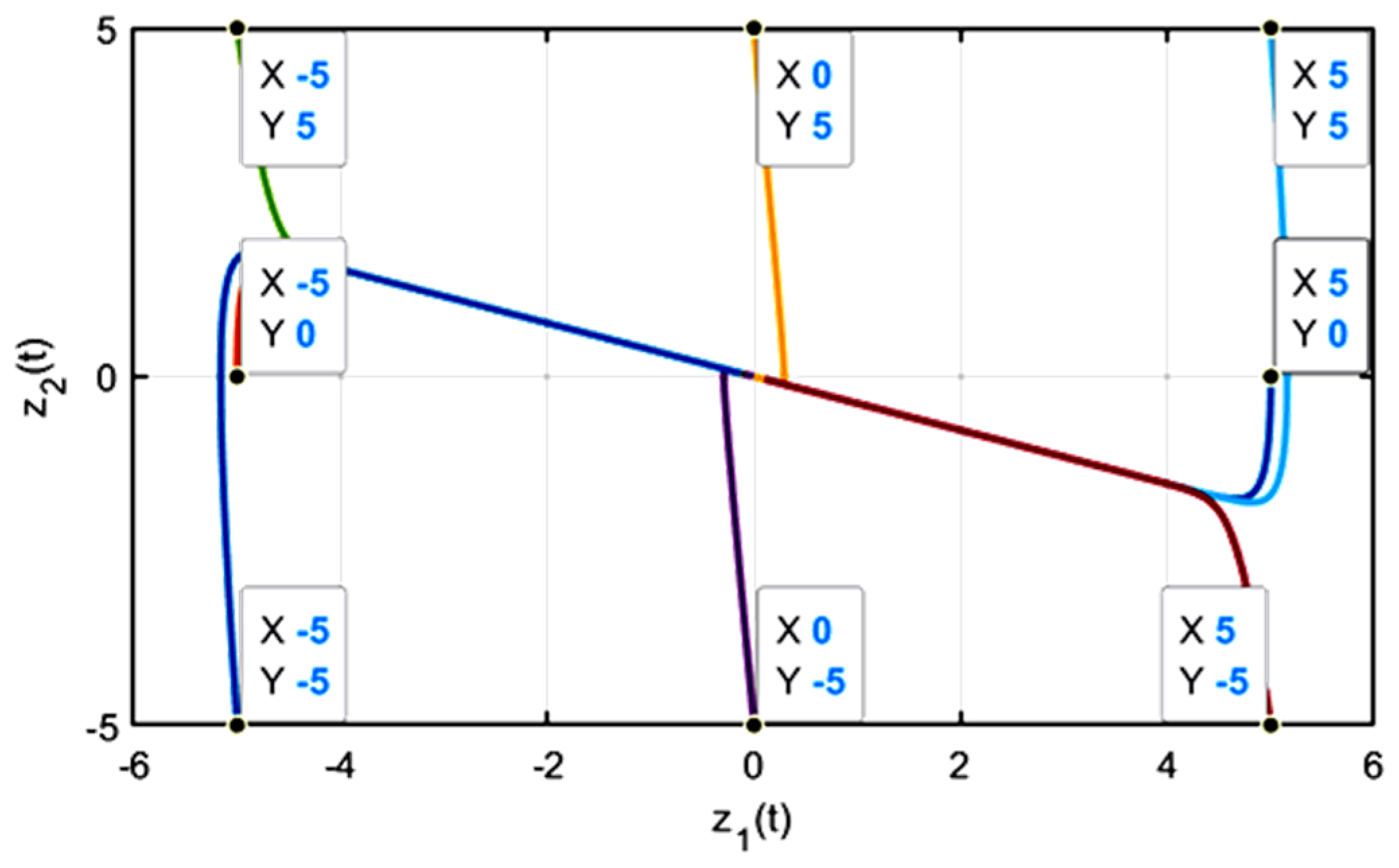
When $i_2\ge 2\sqrt{i_1}$, the eigenvalues of matrix X are all real numbers, and the singular point (0, 0) is a stable node of system S₃. In this paper, eight groups of phase-plane points are selected to analyze the phase-trajectory characteristics under this condition. Set i₁ = 6 and i₂ = 16 and draw its phase-trajectory diagram as follows:

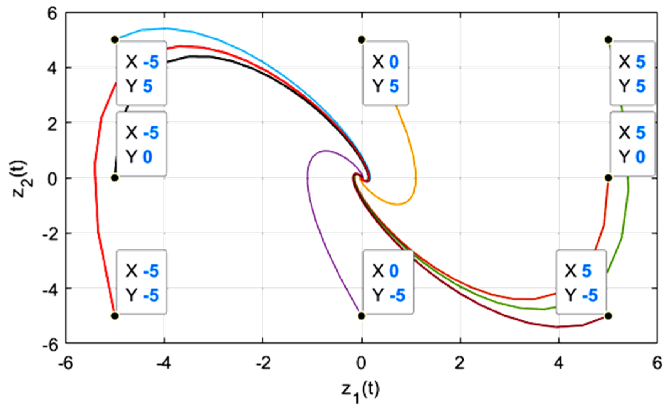
It can be seen, from Figure 6, that the phase-trajectory of the system is smooth and finally directly approaches the origin, and the system state converges stably. Similarly, when, the eigenvalues of matrix X are all imaginary numbers, and the singular point (0, 0) is a stable focus of system S₃. Additionally, we can select eight groups of phase-plane points, set i₁ = 16 and i₂ = 6, and draw their phase-trajectory diagram as shown is Figure 7.

Obviously, differently from the simple and fixed approximation method in the neighborhood of the node, the phase-trajectory in this figure approaches the origin in a spiral form, and the oscillation of the system during the transition process is relatively large. In summary, in order to reduce the overshoot oscillation during the system transition and increase the weight of the linear component in the neighborhood range, in the selection of system parameters, it can be considered to satisfy the constraint.

$$\left\{\begin{array}{l}{a}_{41}\ge 16a_{42}^2\hfill \\ a_{4i}\ge 0.6a_{5i}\hspace{1em}i=1,2\hfill \end{array}\right.$$

(40)

5.3. Parameter Tuning Method of SYSTD

Set the system input signal as Asin(ωt), and define M(A) to describe the nonlinear function f(t) = sys(t):

$$M(A)={\displaystyle \frac{f_1+j{e}_1}{A}}$$

(41)

where e₁ and f₁ are the first-order Fourier coefficients:

$$\begin{array}{l}{e}_1={\displaystyle \frac{1}{\pi }}{\displaystyle {\int }_0^{2\pi }f(t)\cos (\omega t)}\cdot d(\omega t)\\ f_1={\displaystyle \frac{1}{\pi }}{\displaystyle {\int }_0^{2\pi }f(t)\sin (\omega t)}\cdot d(\omega t)\end{array}$$

(42)

Because f(t) is an odd function, e₁, let x₁(t) − r(t) = Asin(ωt), and combined with Equation (42); the function sys(x₁(t) − r(t),a₄₁,a₅₁) can be transformed into the following:

$$M_1(A,a_{41},a_{51})={\displaystyle \frac{1}{\pi }}{\displaystyle {\int }_0^{\pi }sys(A\sin (\omega t),a_{41},a_{51})\sin (\omega t)}\cdot d(\omega t)$$

(43)

Similarly, the function sys(x₂(t)/R,a₄,a₅) can also be transformed into the following:

$$M_2(A,a_{42},a_{52})={\displaystyle \frac{1}{\pi }}{\displaystyle {\int }_0^{\pi }sys(A\sin (\omega t),a_{42},a_{52})\sin (\omega t)}\cdot d(\omega t)$$

(44)

Therefore, the linearized form of the nonlinear system S₂ can be expressed as follows:

$$\left\{\begin{array}{l}{\dot{x}}_1(t)=x_2(t)\hfill \\ {\dot{x}}_2(t)=-R^2[M_1(A,a_{41},a_{51})\cdot (x_1(t)-r(t))+M_2(A,a_{42},a_{52})\cdot {\displaystyle \frac{x_2(t)}{R}}]\hfill \end{array}\right.$$

(45)

From this, the transfer function between the input r(t) and the tracking x₁(t) can be derived as follows:

$$G_{{\displaystyle \frac{x_1}{r}}}={\displaystyle \frac{X_1(s)}{r(s)}}={\displaystyle \frac{R^2\cdot M_1(A,a_{41},a_{51})}{s^2+R\cdot M_2(A,a_{42},a_{52})s+R^2\cdot M_1(A,a_{41},a_{51})}}$$

(46)

Let $T={\displaystyle \frac{1}{R\sqrt{M_1}}}$, $\xi ={\displaystyle \frac{M_2}{2\sqrt{M_1}}}$, ${\omega }_r={\displaystyle \frac{1}{T}}$ then Equation (46) can be simplified as:

$$G_{{\displaystyle \frac{x_1}{r}}}={\displaystyle \frac{1}{T^2{s}^2+2\xi Ts+1}}$$

(47)

where T is the signal period, ξ is the damping coefficient, and ω_T is the cut-off frequency. It should be noted that, when 0 < ξ < 1, system Equation (47) is actually an under-damped system. When the damping is not large enough, chattering may occur.

Therefore, ξ must be greater than 1:

$$M_2\ge 2\sqrt{M_1}$$

(48)

where M₁ > 0 and M₂ > 0 to ensure the stability of the system. The frequency characteristics of the system can be described as follows:

$$G_{{\displaystyle \frac{x_1}{r}}}(j\omega )={\displaystyle \frac{R^2{M}_1}{R^2{M}_1+R{M}_2\cdot (j\omega )-{\omega }^2}}$$

(49)

The amplitude–frequency and phase–frequency characteristics are as follows:

$$L(\omega )=20\log (\left|G_{{\displaystyle \frac{x_1}{r}}}(\omega )\right|)=-20\log \sqrt{{\displaystyle \frac{{\omega }^4+2(M_2^2-M_1^2)R^2{\omega }^2+R^4{M}_1^2}{R^4{M}_1^2}}}$$

(50)

$$\phi (\omega )=\angle \left|G_{{\displaystyle \frac{x_1}{r}}}(\omega )\right|=-\arctan ({\displaystyle \frac{2R{M}_2\omega }{R{M}_1-{\omega }^2}})$$

(51)

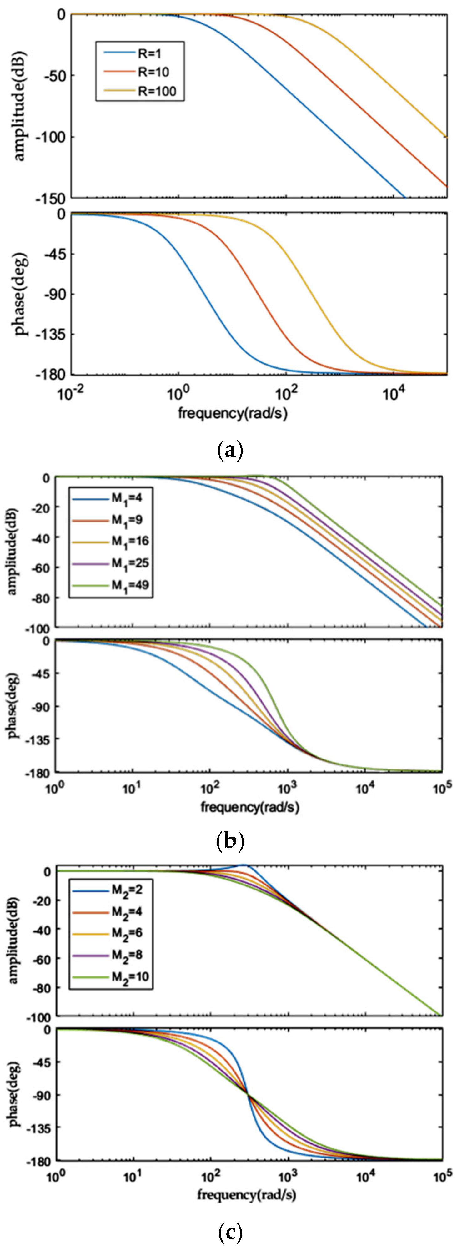
Through simulation, as shown in Figure 8, we observe the influence of the comprehensive parameters of SYSTD on its dynamic characteristics. The results are as follows:

(1)

Influence of the speed factor R on the frequency characteristics. First, fix M₁ and M₂, change R, and then draw the Bode diagram of SYSTD as shown in Figure 8a. It can be seen from the figure that an increase in the value of R can increase the cut-off frequency of the system, which is conducive to the estimation of high-frequency components of the signal and shortens the system response time. However, if the value of R is too large, high-frequency noise will be introduced, reducing the filtering performance of SYSTD. Therefore, the selection of the value of R needs to balance the response speed and filtering performance.

(2)

Influence of parameter M₁ on the frequency characteristics. First, fix M₂ and R, change M₁, and then draw the Bode diagram of SYSTD as shown in Figure 8b. It can be seen that increasing M₁ can increase the cut-off frequency of the system. However, an excessively large M₁ may lead to over-shoot in the high-frequency band of the system, causing survey errors for effective signals and weakening the filtering performance and stability of SYSTD.

(3)

Influence of parameter M₂ on the frequency characteristics. First, fix M₁ and R, change M₂, and then draw the Bode diagram of SYSTD as shown in Figure 8c. An increase in M₂ is beneficial for improving the dynamic response of SYSTD. However, there may be a problem of over-shoot. Moreover, the impact of M₂ on the dynamic performance of SYSTD is more obvious.

It can be seen from the above analysis that, in order to effectively extract the survey signal, it is necessary to first select an appropriate value of R so that the bandwidth of SYSTD can cover the spectrum of the survey signal; then, select appropriate M₁ and M₂ to satisfy Equation (48) and ensure the stability of the system; then, adjust M₁ and M₂ to further balance the contradiction between the filtering ability and the fast response of SYSTD; finally, combined with the basic constraint of Equation (40), select appropriate a₄₁, a₅₁, a₄₂, and a₅₂ to meet the requirements of M₁ and M₂. Generally, the parameters a₅₁ and a₅₂ are adjusted first to adjust the amplitude of SYSTD; then, the parameters a₄₁ and a₄₂ are adjusted to adjust the fast-tracking ability of SYSTD.

5.4. Simulation Analysis of SYSTD Performance

The discrete equation of system S₂ is as follows:

$$\left\{\begin{array}{l}{x}_1(k+1)=x_1(k)+x_2(k)\cdot h+{\displaystyle \frac{1}{2}}{h}^2\cdot u(k)\hfill \\ x_2(k+1)=x_2(k)+h\cdot u(k)\hfill \\ u(k)=R^2[-sys(x_1(k)-r(k),a_{41},a_{51})-sys({\displaystyle \frac{x_2(k)}{R}},a_{42},a_{52})]\hfill \end{array}\right.$$

(52)

Among them, h is the integration step size.

Next, conduct the simulation. Analyze the influence of different set values of parameters R, a₄₁, a₅₁, a₄₂, and a₅₂ on SYSTD through the simulation. Since the movement of the MRC in the horizontal direction is a step-by-step movement, the step distance is set to 1 mm, and the survey signal is close to a sine wave. Therefore, in the simulation experiment, white noise and a sine wave are used as the given signals, and their equations are as follows:

$$r(t)=\sin (t)+\gamma n(t)$$

(53)

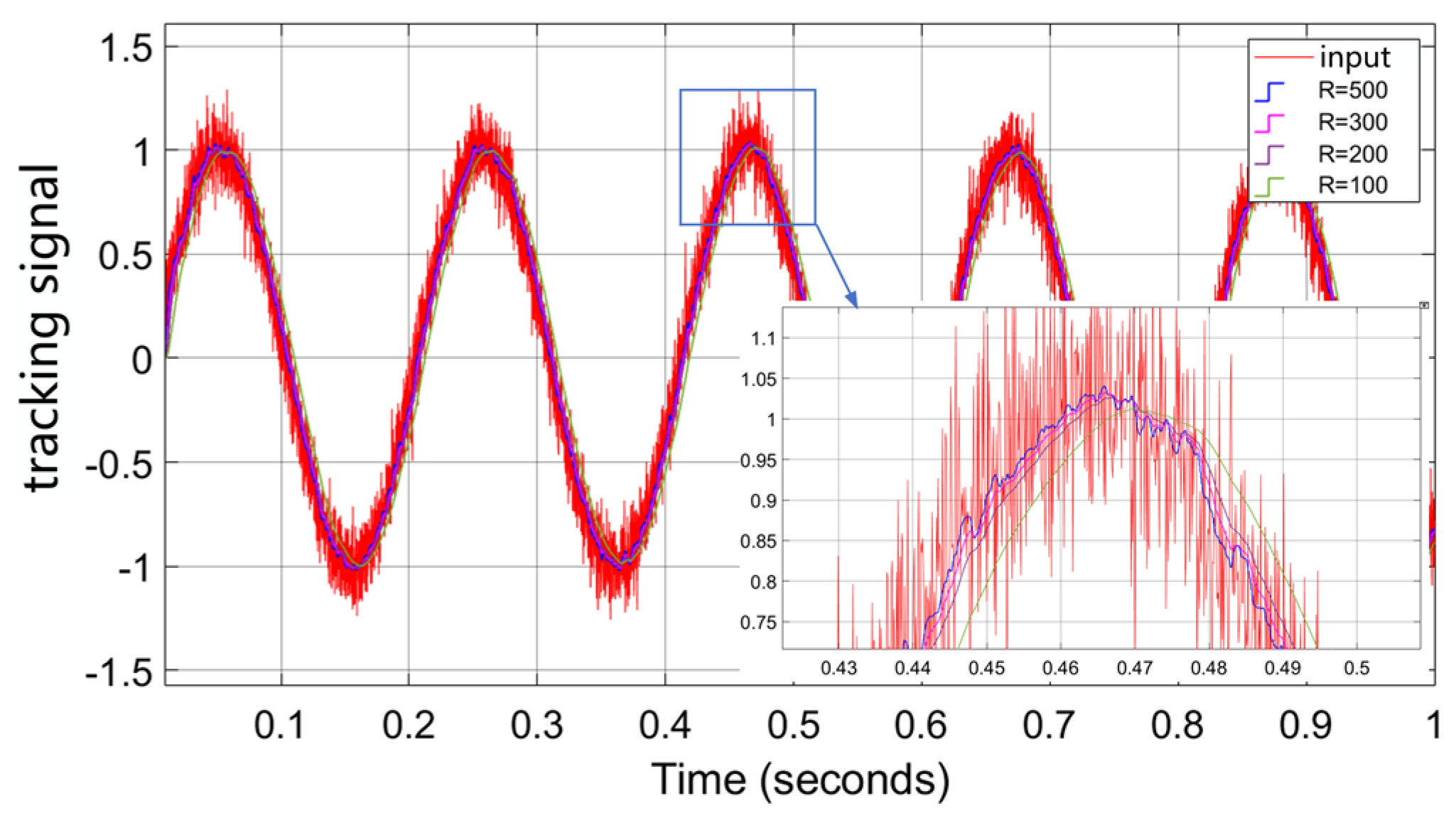
Simulation 1: Influence of the time scale R on the tracking characteristics of SYSTD. According to the constraint conditions of Equations (40) and (48), let a₄₁ = 144, a₅₁ = 16, a₄₂ = 3, and a₅₂ = 1. Take R = 100, 200, 300, and 500, respectively, to simulate the tracking of the given signal by SYSTD. The results are shown in Figure 9. Obviously, the value of R determines the tracking speed of SYSTD. The smaller the value of R, the slower the tracking speed. However, when R > 300, the increase in the tracking speed is not obvious, and at the same time, the oscillation amplitude increases. Therefore, the parameter R has a significant influence on the tracking accuracy of SYSTD. When selecting its value, the balance between the dynamic response and the noise-reduction ability of SYSTD needs to be considered.

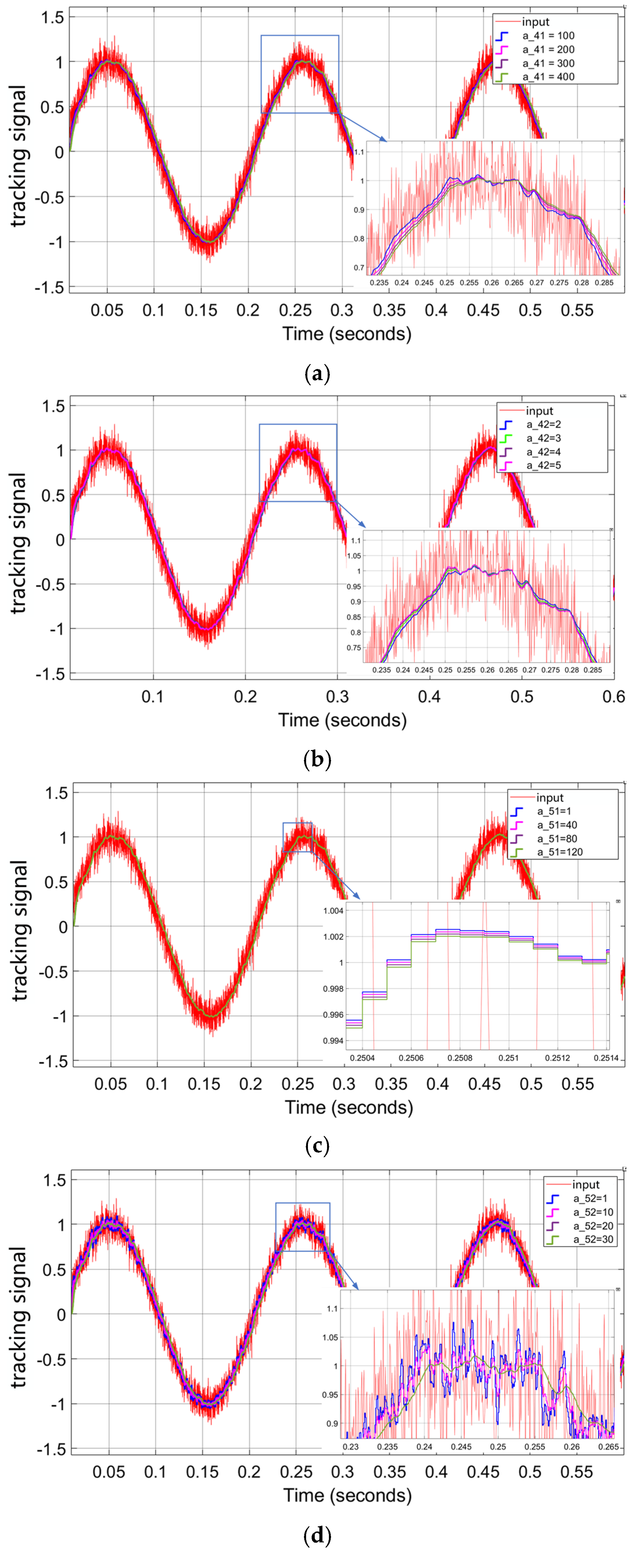
Simulation 2: Influence of the parameters of sys() on the tracking characteristics of SYSTD. As can be seen from Section 5.1, when a₄ is constant, the parameter a₅ directly determines the change in the amplitude of sys(); when a₅ is constant, the parameter a₄ directly determines the change in the tracking rate of sys(). The parameter settings of SYSTD and the results of following the given signal containing random noise are shown in Figure 10.

Obviously, increasing the parameters a₄₁ and a₄₂ can effectively improve the signal tracking speed, but it will result in a loss of tracking accuracy (Figure 10a,c). Additionally, appropriately increasing a₅₁ and a₅₂ can enhance the denoising ability of SYSTD, but it will lead to a loss of tracking speed (Figure 10b,d). Moreover, when the parameters do not meet the constraint conditions required by Equations (40) and (48), it will cause a large overshoot and seriously reduce the tracking accuracy.

To obtain appropriate SYSTD parameters, considering the influence of linear components on the tracking and filtering performance of SYSTD, and, in combination with Simulation 1, first, under the condition of ensuring system stability, roughly select the four parameters of sys(), and then adjust R to meet the requirements of tracking speed and accuracy. Then, based on the phenomena in Simulation 2, adjust a₄ and a₅ to change the amplitude and change rate of sys(), and, thus, adjust the tracking and filtering performance of SYSTD.

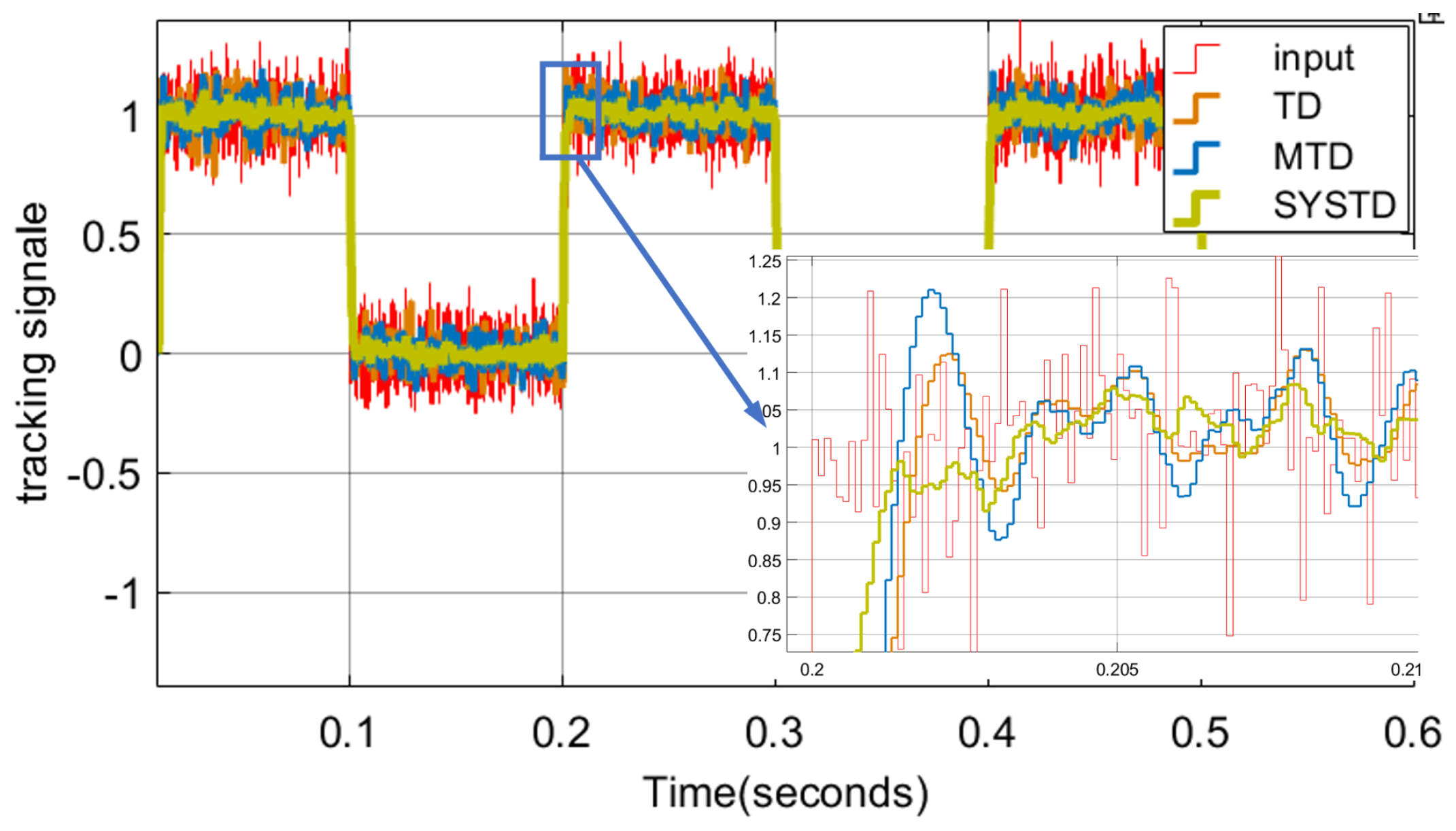
Simulation 3: Performance comparison simulation of TD, MTD, and SYSTD. The parameters of the tracking differentiators selected for comparison are as follows:

(1) TD. The TD and its parameters involved in Literature [1] are used for TD.

(2) MTD [15].

$$\begin{array}{l}\left\{\begin{array}{l}{x}_1(k+1)=x_1(k)+h\cdot x_2(k)+0.5h^2\cdot u(k)\hfill \\ x_2(k+1)=x_2(k)+h\cdot u(k)\hfill \\ u=f(x_1-r,x_2,R,h_0)\hfill \end{array}\right.\\ f(x_1,x_2,R,h_0)=-R^2(a(x_1+{\displaystyle \frac{x_2}{R}})+b(x_1^m+{\displaystyle \frac{x_2^m}{R}}))\end{array}$$

(54)

The advantages and disadvantages of the characteristics of the differential tracker are mainly reflected by its tracking speed and numerical filtering. Under the condition of similar filtering effects, the parameters of three TDs are set as shown in

Table 1. Simulation parameters of three differential trackers: TD, MTD and SYSTD.

TDs	Parameter Settings
TD	R = 1000	h = 0.001
MTD	R = 2	a = 2	b = 2	m = 5
SYSTD	R = 300	a41 = 144	a42 = 3	a51 = 72	a52 = 3

to compare their tracking characteristics for harmonic signals.

The results are depicted in Figure 11 and Figure 12.

For the purpose of clearly observing the comparison results of the tracking characteristics of the three tracking differentiators (TDs), a square-wave signal with a period of 0.2 s and a white-noise signal were superimposed in the simulation. The relevant equation is as follows:

$$r(t)=\sin (t)+\gamma n(t)$$

(55)

Figure 11 and Figure 12 clearly indicate that the SYSTD exhibits the quickest tracking speed and the optimal filtering effect.

5.5. A Method for Estimating the Position of the Mover Iron Core Based on SYSTD

In order to simplify the system structure, the horizontal position of the MRC in this paper is not obtained by survey with a position sensor. Instead, a measuring coil can be wound along the horizontal control coil, and the position feedback signal of the mover core can be estimated from the back electromotive force obtained from the measuring coil.

During the operation process, the MRC is only affected by the electromagnetic suction force, the horizontal thrust force, and the gravitational force. Among them, the magnitude and direction of the electromagnetic suction force are related to the air-gap magnetic field of the magnetic levitation ruler system. The air-gap magnetic field is mainly distributed between the stator yoke and the mover iron core [2].

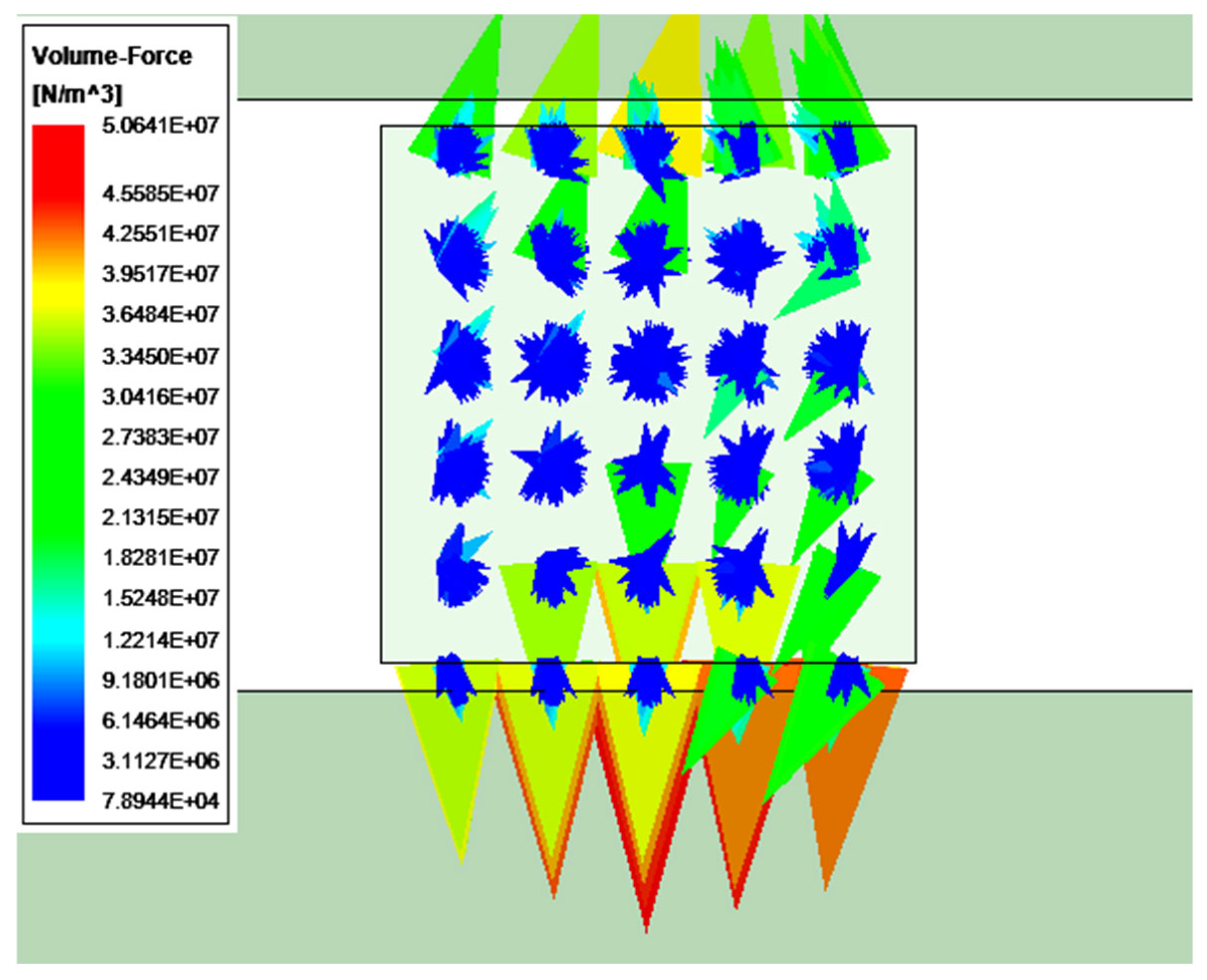
However, there are still residual air-gap magnetic fields on the front and rear sides of the MRC. When the suspension position of the mover is 1.1 mm, the upper and lower residual air-gap magnetic fields are symmetrical. Under the action of this part of the air-gap magnetic field, there are horizontal components in the upward and downward electromagnetic suction forces of the MRC. In this paper, the force analysis of the MRC is carried out by means of MAXWELL. Figure 13 shows the force analysis diagram of the MRC at the left-hand end of the MRC.

As can be seen from the figure, the electromagnetic suction force generated by the air-gap magnetic field is mainly in the Z-direction. However, there are also horizontal components. The horizontal component of the electromagnetic suction force on the front side of the MRC is in the backward direction; the horizontal component of the electromagnetic suction force on the rear side of the MRC is in the forward direction. Most of the horizontal components of the electromagnetic suction force cancel each other out. By means of the MAXWELL field calculator, it is concluded that the total horizontal electromagnetic suction force component of the MRC is approximately 0.04 mN, which is less than 0.1% of the horizontal thrust. Therefore, the horizontal component of the electromagnetic suction force can be neglected.

The horizontal control coil is in contact with the upper and lower surfaces of the MRC. As can be seen from Figure 14, the magnetic field lines of the air-gap magnetic field are perpendicular to the upper and lower surfaces of the MRC and the horizontal control coil in contact with these surfaces.

Thus, an induced-electromotive-force measuring coil can be wound along the horizontal control coil, and the position change of the MRC can be estimated by detecting the induced electromotive force in the measuring coil.

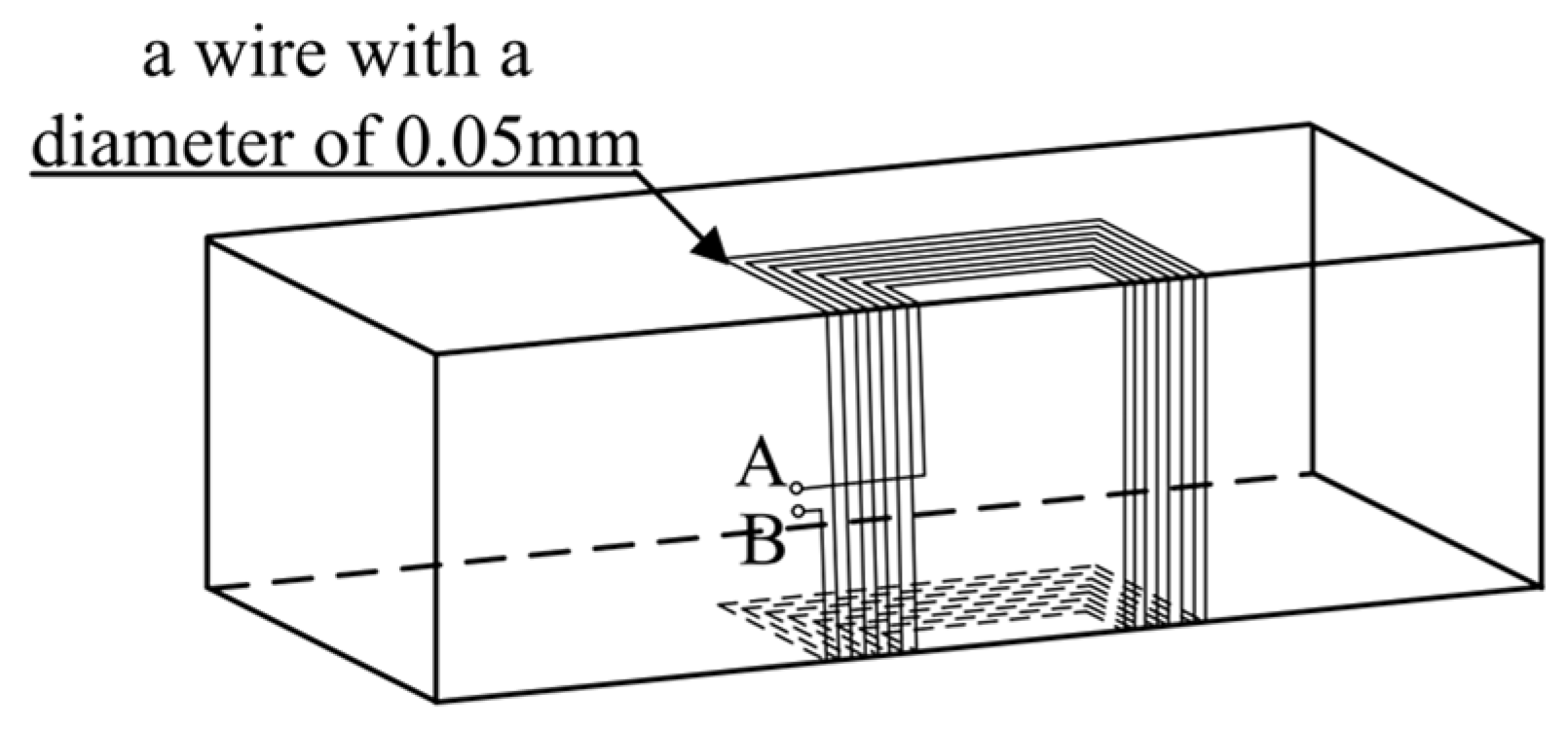
The design objective of the measuring coil is to detect the induced electromotive force, and there is no requirement for the coil current. Therefore, in this paper, enameled wire with a wire diameter of 0.05 mm is chosen to wind the induced-electromotive-force measuring coil along the gaps between the wires of the horizontal control coil, and the number of turns of the coil can reach around 300 as shown in Figure 15.

Figure 15 is a schematic diagram of the winding method of the coil on the left-front side of the mover core. The installation method of the measuring coils on the left-rear side, right-front side, and right-rear side of the mover iron core is the same as this. Among them, the port AB is used to measure the induced electromotive force.

By connecting the two groups of measuring coils on the left side in series, the left-side induced electromotive force e_l can be obtained; by connecting the two groups of measuring coils on the right side in series, the right-side induced electromotive force e_r can be obtained.

The calculation formula for the induced electromotive force when the left-side measuring coil cuts the magnetic field lines is as follows [20]:

$$e_l=BLv=(B_u+B_d)L{\displaystyle \frac{d{S}_l}{dt}}$$

(56)

In the formula, B_u is the air-gap magnetic field strength on the upper-left side of the MRC, B_d is the air-gap magnetic field strength on the lower-left side of the MRC, L is the length of the measuring coil in the air-gap magnetic field, and S_l is the displacement of the MRC. The calculation method of the induced electromotive force e_r is the same as that of e_l, so it will not be repeated here.

In addition, since the measuring coil is wound along the horizontal control coil, the mutual-inductance coefficient k between the measuring coil and the horizontal control coil is infinitely close to 1. Therefore, there is mutual inductance between the measuring coil and the horizontal control coil. According to the mutual-inductance calculation formula, the mutual inductance M can be estimated as follows:

$$M=k\sqrt{L_c\times L_k}$$

(57)

In the formula, Lc is the inductance of the measuring coil; L_k is the inductance of the horizontal control coil. The calculation formula for the inductance is as follows:

$$L={\displaystyle \frac{0.01\times D\times N^2}{\frac{H}{D}+0.44}}$$

(58)

In the formula, L represents the inductance, D represents the diameter of the coil, N represents the number of turns, and H represents the length of the coil.

Thus, it can be calculated that L_c ≈ 12,272 μH, L_k ≈ 122 μH. Therefore, M ≈ 1.2 × 10⁻³ μH. In the measuring coil, the calculation method of the induced electromotive force e_c generated by the mutual inductance is as follows:

$$e_c=-M{\displaystyle \frac{d{i}_c}{dt}}$$

(59)

In the formula, i_c represents the current of the horizontal control coil. The MRC operates in a fixed-step-length stepping motion mode. Therefore, the current of the horizontal control coil is a square wave signal. Here, e_c is the induced electromotive force generated by the mutual inductance. Only at the rising edge and falling edge of the square wave signal will it cause significant fluctuations in e_c. The duration of these fluctuations is influenced by the time constant τ_k of the horizontal control coil.

$${\tau }_k={\displaystyle \frac{L_k}{R}}$$

(60)

R is the equivalent resistance of the horizontal control coil, which is measured to be 1.4 Ω. τ_k is approximately 8.7 μs. To ensure the calculation accuracy, the rising edge and the falling edge of the current in the horizontal control coil are taken as six times the value of τ_k, that is, 52.2 μs. During this period, the frequency of the waveform of e_c is much higher than that of the induced electromotive forces e_l and e_r, and its amplitude is also larger. This issue can be addressed by low-pass filtering for noise reduction. In this paper, SYSTD is used to observe the three signals B_u, B_d, and e_l, respectively, so as to obtain more accurate values of the air-gap magnetic field strength and the induced electromotive force. After substituting these values into Equations (4)–(56), a relatively accurate estimated value of the position of the left end of the MRC can be calculated. The estimated value of the position of the right end of the MRC can be obtained in the same way.

6. ADRC’s ESO, NLSEF, and Disturbance Compensation

6.1. ESO

According to the ADRC law, Equation (18) is rewritten as follows:

$$\left\{\begin{array}{l}{\displaystyle \frac{{\partial }^2{y}_b}{\partial t^2}}=b_y{i}_{cl}+w_y(t)\hfill \\ {\displaystyle \frac{{\partial }^2{\psi }_z}{\partial t^2}}=b_z{i}_{cr}+w_{z1}(t)\hfill \end{array}\right.$$

(61)

where w_y(t) and w_z1(t) are the equivalent disturbances of the system, including coupling and other disturbances. i_cl and i_cr are the control variables. In Equation (61), b_y and b_z are the control parameters of the control variables i_cl and i_cr, respectively.

From this, the current variations of the four horizontal control coils can be obtained. The ADRC can regard w_y(t) and w_z1(t) as the system’s comprehensive disturbance and observe and compensate for them through its ESO. The control variables are selected as follows:

$$\left\{\begin{array}{l}{i}_{cl}={\displaystyle \frac{1}{b_y}}[i_{cl}^{*}-w_y(t)]\hfill \\ i_{cr}={\displaystyle \frac{1}{b_z}}[i_{cr}^{*}-w_{z1}(t)]\hfill \end{array}\right.$$

(62)

After compensation, Equation (20) can be rewritten as follows:

$$\left\{\begin{array}{l}{\displaystyle \frac{{\partial }^2{y}_d}{\partial t^2}}=i_{cl}^{*}\hfill \\ {\displaystyle \frac{{\partial }^2{\psi }_z}{\partial t^2}}=i_{cr}^{*}\hfill \end{array}\right.$$

(63)

After compensation, y_b and ψ_z are decoupled and controllable. Taking y_b as an example, it can be seen from Equation (63) that the system controls y_b through i_cl. In Equation (63), after parameter adjustment, i_cl becomes part of the equivalent disturbance of w_z1(t) and is then observed and compensated by the ESO.

Similarly, when controlling the other degree of freedom ψ_z, i_cr will also cause changes in y_b. In Equation (63), after parameter adjustment, i_cr becomes part of the equivalent disturbance of w_y(t) and is then observed and compensated by the ESO. The ESO of the HCS of the MAR system is as follows:

$$\left\{\begin{array}{l}e(m)=z_1(m)-y(m)\hfill \\ z_1(m+1)=z_1(m)+h[z_2(m)-{\beta }_{e1}e(m)]\hfill \\ z_2(m+1)=z_2(m)+h\left\{z_3(m)-{\beta }_{e2}fal[e(m),0.5,\delta ]+\left.b_{0}u(m)\right\}\right.\hfill \\ z_3(m+1)=z_3(m)-h{\beta }_{e3}fal[e(m),0.25,\delta ]\hfill \end{array}\right.$$

(64)

where:

$$fal(e,a_1,\delta )=\left\{\begin{array}{ll}{\left|e\right|}^{a_1}sign(e)\hfill & \hfill \left|e\right|>\delta \\ {\displaystyle \frac{e}{{\delta }^{1-a_1}}}& \hfill \left|e\right|\le \delta \end{array}\right.$$

where z₁(m), z₂(m) and z₃(m) are the state variables of the ESO. z₁(m) and z₂(m) are used to track the state variables of the system, and z₃(m) is used to track the state variable of the total disturbance. β_e1, β_e2, and β_e3 are the gains of the ESO. a₁ and δ are undetermined parameters. If a₁ is less than 1, the function has nonlinear characteristics such as small gain for large errors and large gain for small errors. δ represents the linear range, aiming to avoid oscillation caused by large gain for extremely small errors.

6.2. NLSEF

For the HCS of the MAR system, the NLSEF of the following form is adopted:

$$\left\{\begin{array}{l}{e}_1(m+1)=x_1(m+1)-z_1(m+1)\hfill \\ e_2(m+1)=x_2(m+1)-z_2(m+1)\hfill \\ u_0(m+1)={\beta }_{f1}fal[e_1(m+1),a_2,{\delta }_{f1}]+{\beta }_{f2}fal[e_2(m+1),a_3,{\delta }_{f1}]\hfill \end{array}\right.$$

(65)

where e₁(m) and e₂(m) are the deviation and its derivative between the expected transition process and the estimated value of the system output. a₂, a₃, and β_f1 are the relevant parameters of fal. u₀ is the output of the NLSEF, and b₀ is the compensation coefficient.

6.3. Disturbance Compensation

In reality, when the MRC moves horizontally, it may encounter sudden load changes, interference at a certain frequency, and external force impacts,; noise signals may also penetrate into the displacement signal, affecting the control.

The ESO is used to track the representative disturbance state variable z₃(m) extended from the original system. The control variable is used to compensate for the disturbance and is transformed into an integral-series control variable. The control variable is as follows:

$$u(m+1)={\displaystyle \frac{u_0(m+1)-z_3(m+1)}{b_0}}$$

(66)

7. Parameter Tuning Method of the HCS of the MAR System

Through numerous simulation experiments and prototype testing experiments, this paper summarizes the parameter tuning method of the HCS of the MAR system:

The parameter tuning method of SYSTD is described in Section 5.3.

ESO Parameter Tuning: There are three parameters to be tuned in the ESO, namely, β_e1, β_e2, and β_e3. β_e3 is the most important among the three parameters.

When tuning the parameters, first, select the parameter β_e3. If β_e3 is too small, the observation accuracy of z₃(m) will be insufficient, and z₁(m) and z₂(m) will lag behind x₁(m) and x₂(m). If β_e3 is too large, it will increase system fluctuations and even cause system oscillation. Therefore, β_e3 is adjusted first to ensure the accuracy of the ESO.

Then, adjust β_e1 and β_e2 from small to large to reduce the oscillation of the ESO output. Since there is coupling in the horizontal system of the MAR system, these two parameter values should be as small as possible while ensuring the stable output of the ESO.

In addition, δ has a significant impact on β_e1, β_e2, and β_e3. Before adjusting these three parameters, the value of δ needs to be determined first. In this paper, δ = h.

NLSEF Parameter Tuning: There are three parameters to be tuned in the NLSEF, namely, β_f1, β_f2, and b₀. b₀ is the coefficient of the control variable u. The adjustment methods of β_f1 and β_f2 are similar to those of PD parameters.

8. Simulation Analysis of the HCS of the MAR System

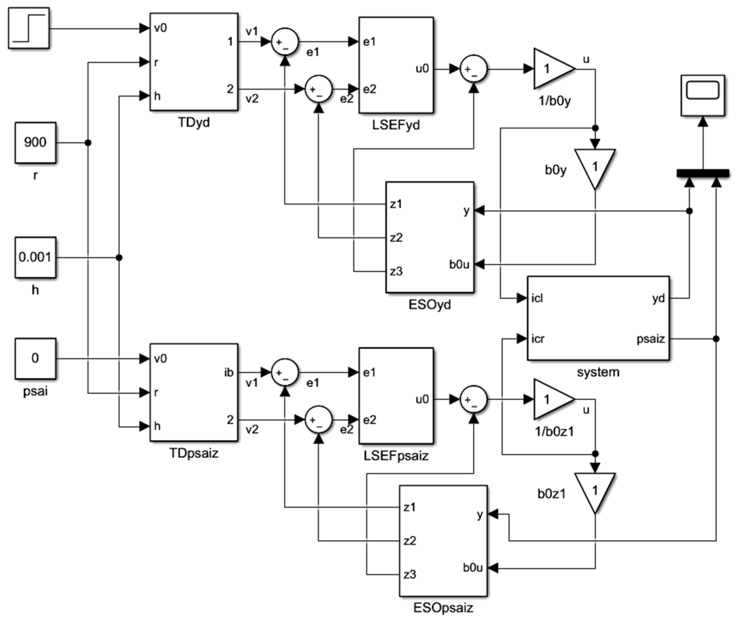
To facilitate the simulation analysis of the feasibility of the HCS of the MAR system, a simulation model of the HCS is built using Simulink (10.1(R2020a)), as shown in Figure 16.

The parameters of the MRC of the MAR system are J_α = 1.49 × 10⁻² kg·m², the lever arm r = 0.1275 m, and the mass m = 1.83 kg. The parameter values of SYSTD are shown in 5.4. The other main parameters of the ADRC are shown in

Table 2. Other main parameters of the ADRC.

Name	Value	Name	Value	Name	Value
βe1	150	βf1	27	a3	0.5
βe2	1078	βf2	0.02
βe3	819	a2	0.25

.

Suppose at t = 0 s, when the Y-direction coordinate value of the MRC is 0, a sudden given value y_d* = 1 mm and ψ_z* = 0 rad/s are applied to detect the response characteristics of the MAR system when the MRC moves within one step during displacement detection.

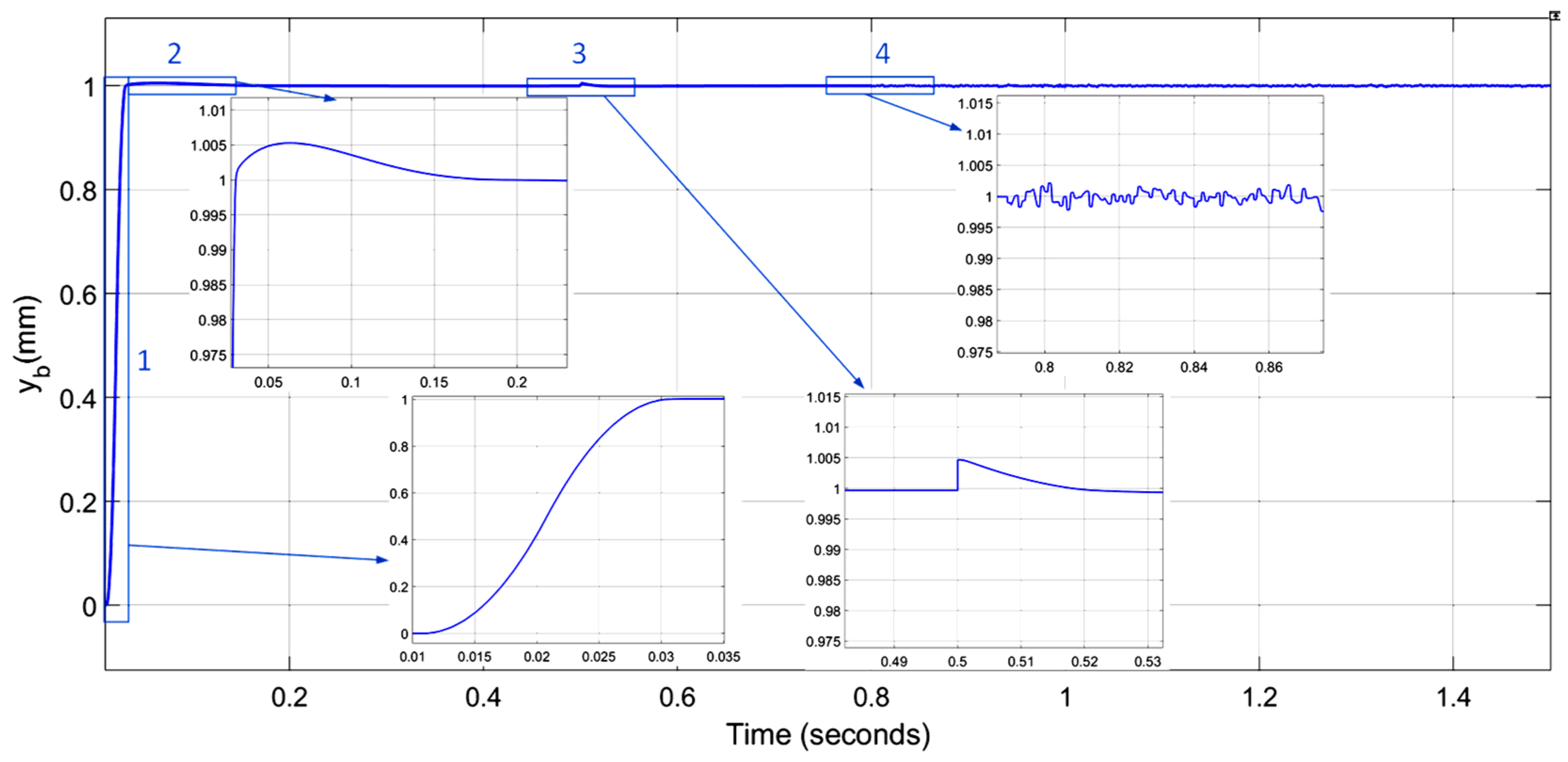
In addition, at t = 0.5 s, a position disturbance of y_b = 0.005 mm is added, and, at t = 0.8 s, white-noise interference is added to simulate external interference. The simulation results are shown in Figure 17.

Figure 17 is divided into four regions for detailed analysis:

The partial enlarged view of Region 1 is shown in Figure 17. It can be seen that the MRC can reach the displacement given value of 1 mm (i.e., one step) in about 0.03 s after starting. Within one step, the MRC first accelerates from a stationary state, moves 0.5 mm, and then decelerates to a stop. Additionally, the displacement curve within one step is relatively smooth, which is conducive to improving the accuracy of the MAR system after subdivision.

A partially enlarged view of Region 2 is shown in Figure 17. It can be seen that the MRC will have an overshoot at the end of each step. The overshoot does not exceed 6 μm and is corrected within 0.2 s.

A partially enlarged view of Region 3 is shown in Figure 17. It can be seen from the figure that the disturbance can be quickly eliminated.

A partially enlarged view of Region 4 is shown in Figure 17. The white noise has little impact on the HCS.

As can be seen from Figure 17, the HCS of the MAR system has strong robustness, and the positioning accuracy can reach ±5 μm.

The following is true as is known from Reference [2]:

$$m{\displaystyle \frac{d^{2}S}{d{t}^2}}=B{I}_{L}L$$

(67)

By taking the integral of both sides of Equation (67) from 0 to t and ignoring the constant term, the following equation can be obtained:

$$S={\displaystyle \frac{nB{I}_{L}L}{2m}}{t}^2$$

(68)

where n represents the number of turns, B represents the magnetic induction intensity in the air-gap, I_L represents the current of the horizontal control coil, L is the length of the horizontal control coil in the air-gap magnetic field, and m is the mass of the MRC. Assuming these quantities are constants, the relationship between the displacement S of the MRC and time t is a quadratic function, which is consistent with the simulation results in Figure 17.

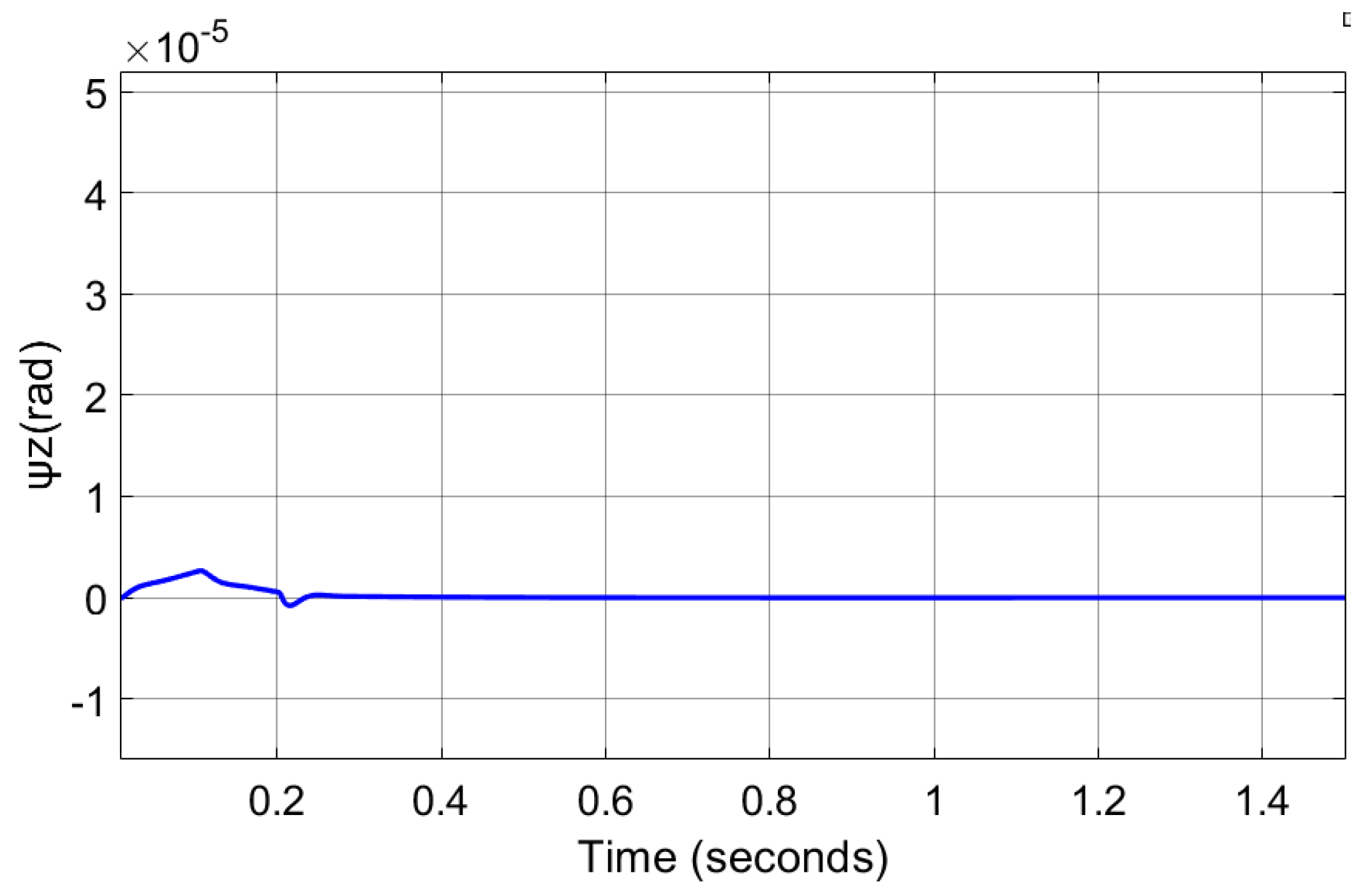
Figure 18 is the simulation diagram of the horizontal rotation angle of the MRC. It can be seen from the above two figures that, when the MRC starts, there is a slight angular deviation on the Z-axis. The angular deviation is corrected in about 0.2 s, and the movement distances at both ends are basically the same, indicating that the HCS has achieved decoupling control.

9. Experiment and Test of the HCS

To verify the control effect of the HCS, a horizontal positioning experiment of the MRC was carried out on the MAR system test platform shown in Figure 19.

The hardware platform comprised an MAR, horizontal control coil, coil driving circuit, sensors, and levitation control system [1]. In the experimental setup, a grating ruler boasting an accuracy of 0.1 μm and a resolution of 0.01 μm was employed. It was rigidly connected to the MRC to accurately calibrate the horizontal displacement of the MRC. y_d was captured by measuring coils. The angle sensor is affixed to the MRC using an adhesive. ψ in Figure 19 was captured by an angle sensor.

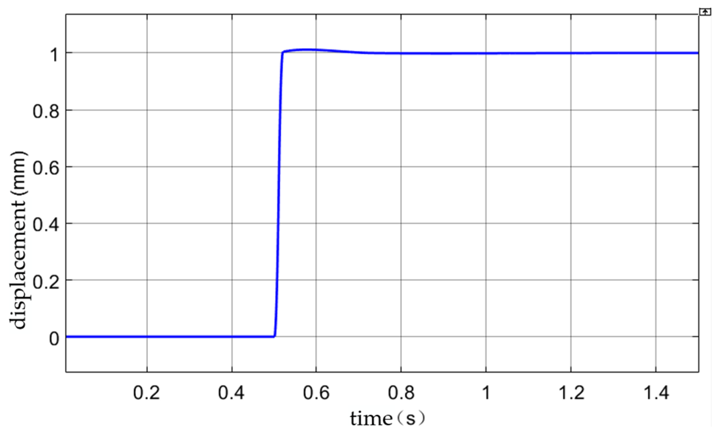
Figure 20 shows the measured start-up response curve of the MRC. It can be seen from the curve that the MRC exhibits good response speed and stability during the start-up process. In a very short time, the MRC can quickly reach the preset horizontal position and ensure accurate positioning throughout the process.

As shown in Figure 20, at t = 0.5 s, the horizontal position set value of the MRC was adjusted to 1 mm, that is, one step. The horizontal position of the MRC reached the set value within t = 0.58 s with no obvious overshoot. After t = 0.75 s, the horizontal position of the MRC stabilized at the set horizontal position value, with an error within ±2 μm. The adjustment speed is slightly slower than that shown in the simulation.

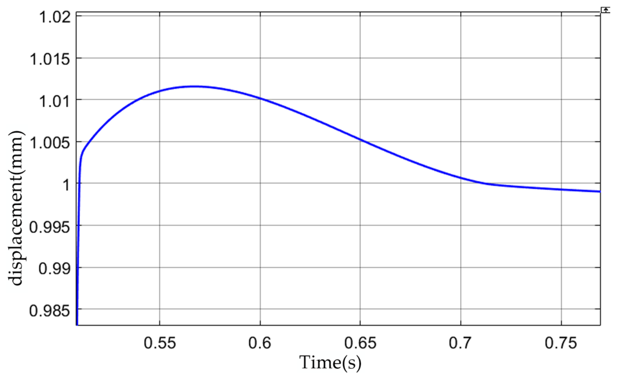
It can be seen from Figure 21 that the overshoot of the actual HCS is more than twice that of the simulation. The MRC begins to enter a stable state at about t = 0.72 s, which is 0.02 s more than that in the simulation. After that, there is still an error, but it is less than ±2 μm.

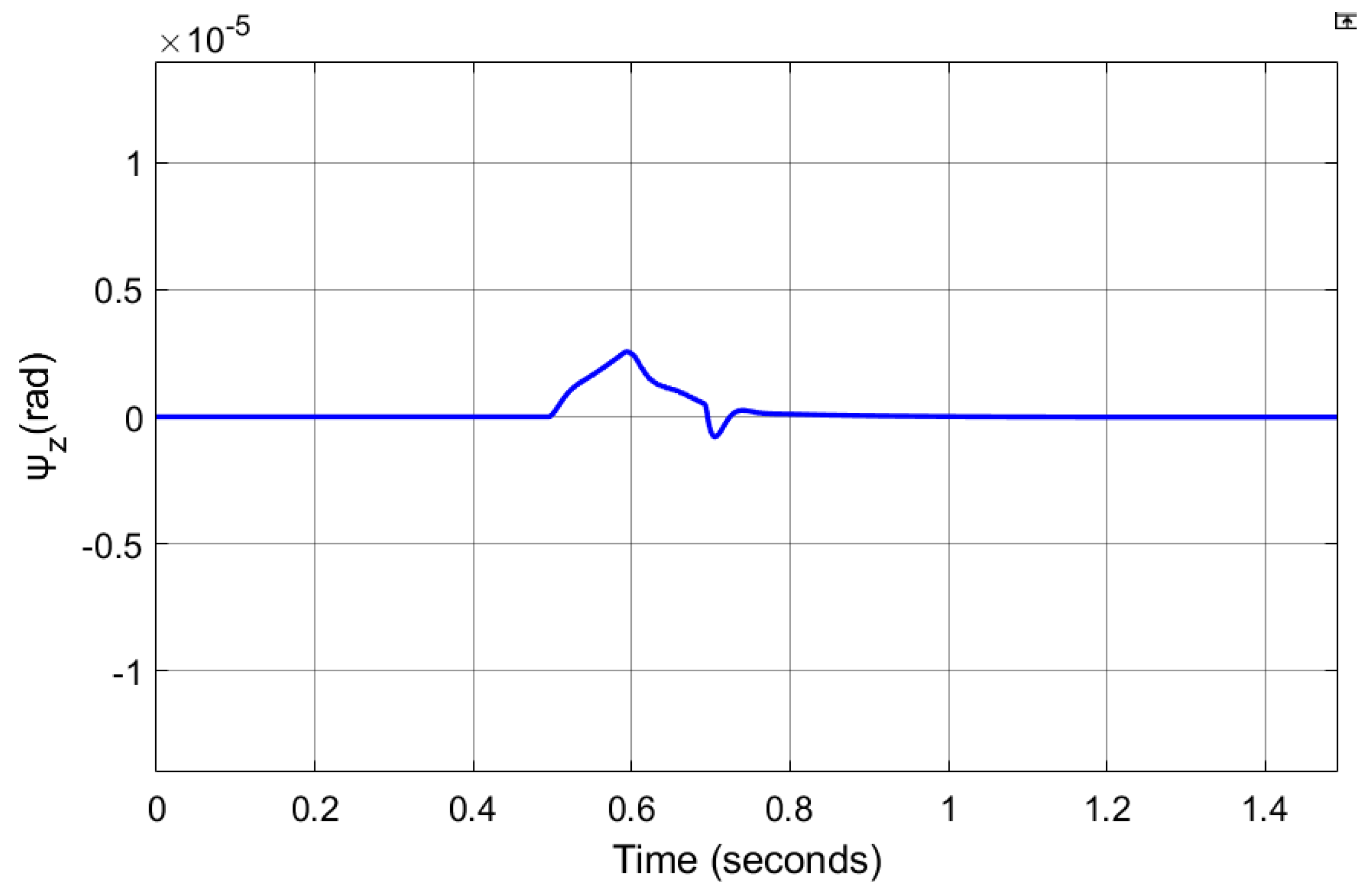
As shown in Figure 22, at t = 0.5 s, the deflection angle of the MRC changes. At this time, the horizontal position set value of the MRC also changes suddenly, and the HCS starts to adjust the horizontal position of the MRC. At t = 0.6 s, the deflection angle reaches its maximum value. Before t = 0.8 s, the deflection angle returns to zero degrees, and the transition process of the suspension position is also completed. The MRC stabilizes at the new horizontal position.

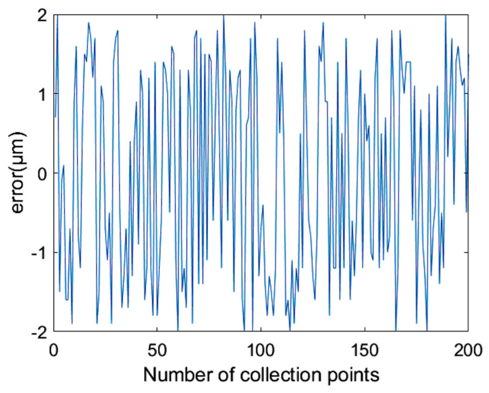
Obviously, there is strong coupling when controlling the horizontal positions of the left and right ends of the MRC. The transition process of the horizontal position will interfere with the deflection angle of the MRC. However, the HCS can eliminate the interference in about 0.22 s, complete one step. The control accuracy can reach ±2 μm under 200 repeated trials, as shown in Figure 23. Therefore, the HCS effectively achieves decoupling control and has excellent robustness.

The performance comparison among conventional linear active disturbance rejection control (LADRC), PID control methods, and the proposed improved active disturbance rejection control (I-ADRC) method is summarized in

Table 3. Comparative performance metrics of control methods in nonlinear and coupled systems.

Control Method	Positioning Accuracy (μm)	Setting Time (ms)	Overshoot (%)	Applicability to Nonlinear System
Proposed ADRC	±2	580	1.2	Yes (Designed for coupling)
PID [8]	±10	1200	8.5	No (Linear assumption)
LADRC [10]	±5	800	0.25	Partial (Limited decoupling)

.

10. Discussion

This paper focuses on the autonomous displacement of the MAR system and has achieved innovative results in system control algorithms and structural optimization. The proposed new differential tracker, SYSTD, effectively solves the problem of tracking the position feedback signal of the MRC. SYSTD is constructed based on specific elementary functions, and its stability has been verified through theoretical derivation. Through phase-plane analysis, a theoretical basis for its parameter selection is provided, and the detailed parameter tuning method enhances its operability in practical applications. Simulation results show that SYSTD achieves a good balance between tracking speed and stability. Compared with traditional TD and MTD, it has a faster tracking speed and better filtering effect. This not only improves the tracking accuracy of the MAR system for the position feedback signal of the MRC but also provides new ideas for the control algorithm design of other similar systems. In terms of system structure optimization, the method of estimating the position of the MRC by winding survey coils along the horizontal control coils realizes sensorless control. This innovation simplifies the system structure, reduces costs, and improves system reliability. Combined with the precise observation of relevant signals by SYSTD, the accuracy of position estimation is further improved, providing a more advantageous solution for the practical application of the MAR system. However, this paper also has certain limitations. During the experiment, it was found that the overshoot of the actual system is larger than that of the simulation results, and the time to enter a stable state is also longer. This may be due to the more complex interference factors in the actual environment, which are difficult to fully simulate in the simulation. Future research can consider further optimizing the control algorithm to enhance its adaptability to complex actual environments and improve the stability of system performance.

This study has limitations: (1) environmental disturbances (e.g., electromagnetic noise) may degrade performance in industrial settings; (2) long-term thermal effects on coil resistance were not modeled. Future work will integrate real-time disturbance observers and temperature compensation modules. Additionally, we plan to extend the control framework to 3D multi-axis coordination for complex trajectory tracking.

11. Conclusions

This research involved an in-depth analysis and optimization of the HCS of the MAR system. By establishing a mathematical model, it is clear that the system is a nonlinear and strongly coupled system with two inputs and two outputs.

The HCS designed based on ADRC utilizes its characteristics of a low requirement for modeling accuracy and effective compensation for comprehensive disturbances to achieve decoupling control of the system. In response to the problem that the traditional TD cannot stably track the high-frequency position feedback signal of the MRC, a new differential tracker, SYSTD, is constructed. The simulation shows that SYSTD balances rapidity and stability well and significantly improves the tracking accuracy of the position feedback signal.

At the same time, the proposed sensor-less control method simplifies the system structure and improves the accuracy of position estimation by winding survey coils to estimate the position of the MRC.

Verified by simulation and experiments, the improved HCS of the MAR system has good dynamic and static characteristics and robustness. The positioning accuracy can reach ±5 μm in simulation, and the control accuracy can reach ±2 μm in experiments. It can effectively achieve decoupling control. The research results of this paper lay a solid foundation for the practical application of the MAR system and are expected to promote the wide application of this technology in fields such as coordinate survey.

Future work will integrate temperature compensation and extend the framework to include 3D multi-axis coordination.