Article

Predicting Filter Medium Performances in Chamber Filter Presses with Digital Twins Using Neural Network Technologies

by
Dennis Teutscher
1,2,*,
Tyll Weber-Carstanjen
3,
Stephan Simonis
1,4 and
Mathias J. Krause
1,2,4
1
Lattice Boltzmann Research Group, Karlsruhe Institute of Technology, 76131 Karlsruhe, Germany
2
Institute for Mechanical Process Engineering and Mechanics, Karlsruhe Institute of Technology, 76131 Karlsruhe, Germany
3
Simex Filterpressen und Wassertechnik GmbH & Co. KG, 75365 Calw, Germany
4
Institute for Applied and Numerical Mathematics, Karlsruhe Institute of Technology, 76131 Karlsruhe, Germany
*
Author to whom correspondence should be addressed.
Appl. Sci. 2025, 15(9), 4933; https://doi.org/10.3390/app15094933
Submission received: 26 March 2025 / Revised: 21 April 2025 / Accepted: 28 April 2025 / Published: 29 April 2025

Abstract

:
Efficient solid–liquid separation is crucial in industries like mining, but traditional chamber filter presses depend heavily on manual monitoring, leading to inefficiencies, downtime, and resource wastage. This paper introduces a machine learning-powered digital twin framework to improve the operational flexibility and predictive control of a traditional chamber filter press. A key challenge addressed is the degradation of the filter medium due to repeated cycles and clogging, which reduces filtration efficiency. To solve this, a neural network-based predictive model was developed to forecast operational parameters, such as pressure and flow rates, under various conditions. This predictive capability allows for optimized filtration cycles, reduced downtime, and improved process efficiency. Additionally, the model predicts the filter medium’s lifespan, aiding in maintenance planning and resource sustainability. The digital twin framework enables seamless data exchange between filter press sensors and the predictive model, ensuring continuous updates to the training data and enhancing accuracy over time. Two neural network architectures, feedforward and recurrent, were evaluated. The recurrent neural network outperformed the feedforward model, demonstrating superior generalization. It achieved a relative L 2 -norm error of 5 % for pressure and 9.3 % for flow rate prediction on partially known data. For completely unknown data, the relative errors were 18.4 % and 15.4 % , respectively. Qualitative analysis showed strong alignment between predicted and measured data, with deviations within a confidence band of 8.2 % for pressure and 4.8 % for flow rate predictions. This work contributes an accurate predictive model, a new approach to predicting filter medium cycle impacts, and a real-time interface for model updates, ensuring adaptability to changing operational conditions.

1. Introduction

Filter presses play a critical role in numerous industries, including wastewater treatment, pharmaceuticals, and mining, by efficiently separating solids from liquids. A chamber filter press is a specific type of filter press that operates by pumping slurry into a series of recessed chambers lined with filter cloth. As pressure builds, liquid passes through the cloth and exits the system, while solids are retained to form filter cakes. This design enables high solid–liquid separation efficiency and is widely used in industrial applications due to its robustness and reliability. In the mining sector, where vast quantities of ore are processed daily and water consumption is significant [1], filter presses are indispensable for reducing fluid content in the separated material [2]. This reduction not only minimizes water usage but also mitigates the risks associated with sludge storage, such as dam failures [3]. As mining operations can have a big impact on the environment [4], it faces increasing environmental regulations and demands for sustainability. The optimization of filtration processes through innovations such as augmented reality (AR) and machine learning (ML) presents a significant opportunity to enhance automation, monitoring, and operational efficiency. Machine learning has been widely recognized for its role in predictive analytics and adaptive control in filtration systems [5,6]. In parallel, recent work has demonstrated the potential of AR to support real-time process monitoring, operator training, and decision-making in industrial environments [7,8,9], suggesting further possibilities for its integration into filtration processes. By embedding predictive capabilities within filter press systems, operators can achieve higher precision in process control, leading to greater efficiency and better quality outputs. This idea has been researched through different approaches. For example, Landman et al. [10] used the theory of compressive rheology to predict the filtration time and maximize suspension throughput. Other approaches utilize neural networks (NNs) to predict metrics such as filtered volume [11], flow rate, and turbidity [12], or to predict and optimize particle counts [13]. NNs are particularly suited for modelling complex tasks due to their capability as universal function approximators, allowing them to capture intricate, non-linear relationships within diverse datasets [14]. Their adaptability and effectiveness have been demonstrated across various domains, including engineering, medical, and industrial applications, where they are used for tasks such as pattern recognition, classification, and prediction. Furthermore, recent works highlight their effectiveness in time-series forecasting and industrial prediction problems, showcasing their flexibility in real-world scenarios [15]. Another possibility is the application of computational fluid dynamics (CFD). For instance, Spielman et al. [16] employed a numerical model based on the Brinkman equation to predict pressure drops and filtration efficiency. Highly performant simulation software based on the lattice Boltzmann method (LBM) could also be utilized for this purpose [17]. However, the setup required for such simulations can be very challenging, covering aspects such as sedimentation [18,19,20], behaviour during the filling phase, and actual filtering processes aided by porous areas [21,22]. Additionally, while LBM are significantly faster than other simulation approaches [23,24], the results are still not available in real time.
Traditional filter press operations are highly dependent on manual monitoring and adjustments, which often result in inefficiencies, human errors, and increased downtime. Predicting performance parameters such as pressure and flow rates in real time is challenging, as these variables are influenced by fluctuating operating conditions and the state of the filter medium. The condition of the filter medium, particularly its level of clogging and the number of operational cycles it has undergone, significantly affects performance [25,26,27,28,29]. Filter press dynamics are inherently complex due to the interplay of multiple non-linear variables, including pressure, flow rate, and cake resistance, which evolve over time. In addition, fluctuations in components, such as membrane pumps, introduce noise, further complicating real-time predictive analysis. Existing data acquisition systems often lack the ability to seamlessly interface with advanced ML algorithms, limiting operational flexibility and optimization potential. According to the work of McCoy et al. [6], one problem in using ML in the mining sector is the missing amount of data to train a model. Addressing these challenges requires the integration of real-time data analytics with robust ML capabilities to enable smarter and more adaptive process control.
To address these challenges, this work proposes a machine learning-based predictive framework embedded within a digital twin (DT) architecture, a concept that refers to a virtual representation of a physical system, enabling real-time monitoring, analysis, and optimization of its operations through the integration of real-time data and predictive models [30]. The DT is designed to enable real-time estimation of key process variables, specifically pressure and flow rate, while also tracking the condition of the filter medium over successive cycles. By integrating both historical and live data, the approach mitigates the data scarcity issue and enables more robust, adaptive control strategies. The predictive model reduces reliance on manual intervention, enhances process stability, and helps determine the optimal point for filter cloth replacement, improving long-term efficiency and sustainability. By addressing both real-time and historical data, the model can assist operators in determining optimal filter medium utilization, thereby enhancing efficiency and sustainability. Key performance metrics, including root mean square error (RMSE) and mean square error (MSE), are used to evaluate the accuracy of the model in training and validation datasets. The contributions of this work can be summarized as follows. First, a machine learning-based digital twin framework is developed for a chamber filter press, enabling accurate prediction of key operational parameters such as pressure and flow rate across varying experimental configurations. Second, the proposed framework includes predictive modelling of the filter medium efficiency, allowing for proactive maintenance planning and supporting long-term resource sustainability. Finally, the architecture supports seamless data exchange and continuous model updates, ensuring adaptability to evolving operational conditions. In the remainder of the paper, first the methodology is described in Section 2, which contains the experimental setup, parameter selection, and the architecture of the DT, as well as the NN model. Lastly, the results are discussed in Section 3 and conclusions are drawn in Section 4.

2. Methodology

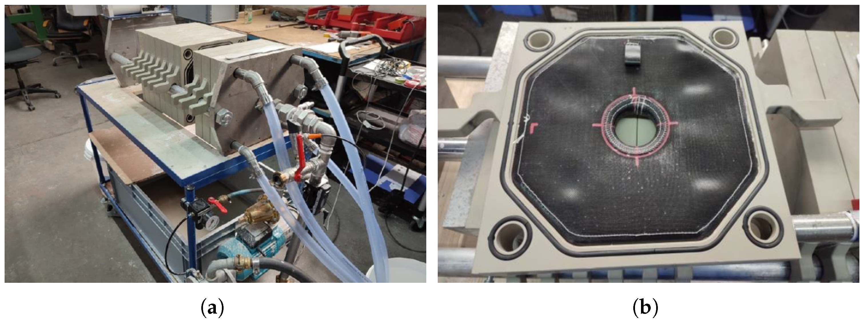
2.1. Experimental Setup of the Chamber Filter Press

The chamber filter press used in this study has a plate size of 300 mm, a compromise between typical small-scale test presses (150 mm plate size) and larger versions (up to 1000 mm). This size is compatible with existing infrastructure, requires manageable suspension quantities, and is portable. The press is equipped with a membrane pump and a manually operated hydraulic cylinder, common configurations in industry, ensuring transferability of results. The setup includes a central inlet and outlets in each corner of the plates, maintains uniform conditions across the press, and aligns with industrial applications, such as automotive paint-sludge treatment and marine scrubber systems. This design ensures leak-tightness and consistent filtrate flow, enhancing reproducibility. Air blowing for filter cake removal is controlled through adjustable valves, allowing for variable air flow. Figure 1 shows the experimental setup next to the filter chamber with the filter cloth.
In order to ensure consistency and reproducible results that can be used to train a model, a suspension consisting of a mixture of water and perlite was used as the test material.
The filter cloth used in the experiments had a throughput capacity of 5 l dm 2 · min . During each experiment, filtration was performed under controlled conditions to evaluate key parameters such as filtrate flow rate, pressure, filter cake formation, and overall filtration performance. The filtration process continued until a specified end point, such as a defined pressure or filtrate volume. Air blowing was then applied to remove the filter cake, with the air flow rate adjusted via the system’s valves.

2.2. Parameter Selection

Effective training of an NN for a chamber filter press requires selecting input and output variables that capture the intricate dynamics of the filtration process. The flow rate of the filtrate and the operating pressure were chosen as the primary output variables because they are key indicators of the filtration performance. As filtration progresses, the pressure gradually increases, while the flow rate decreases, eventually approaching zero. This decrease in flow, combined with an increase in pressure, signals that the filter chambers are filled with accumulated solids, indicating the end of the filtration cycle. Accurately predicting these variables allows one to monitor process efficiency in real time.
The input variables selected reflect various factors that influence the dynamics of filtration. The number of filter chambers directly impacts the filtration capacity, with a larger number of chambers enabling higher throughput. Filtration time captures the time-dependent evolution of flow and pressure, which is critical to understanding the progression of the cycle. The concentration of solids in the suspension plays a crucial role, as higher concentrations lead to a faster accumulation of solids within the chambers, affecting pressure dynamics and accelerating clogging. Another important input is the cycle count of the filter cloths, as repeated use degrades their performance, reducing the filtration efficiency over time. In addition, the maximum operating pressure sets the upper limit of the system, influencing the pressure and flow profiles throughout the process.
To enhance the generalization capability of the model, we constructed a training dataset to cover a wide range of operational conditions, including variations in chamber configurations, solid concentrations, and filter cloth usage. This comprehensive approach ensures that the model can accurately predict filtration outcomes across diverse scenarios, supporting effective, data-driven process control and optimization.

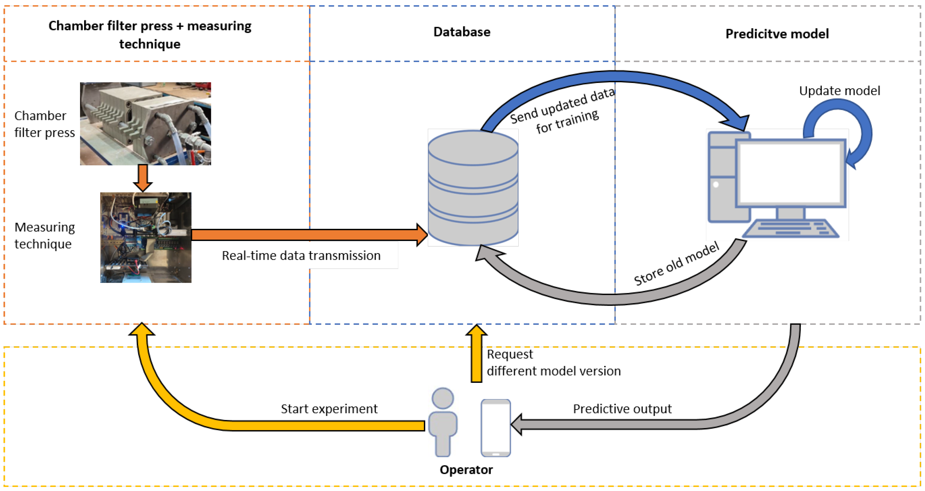
2.3. Digital Twin Architecture

The concept of the DT for the chamber filter press revolves around a continuously improving NN model that is updated with new training data as the filter press operates. This dynamic updating process ensures that the model predictions become increasingly reliable and accurate over time. As illustrated in Figure 2, the operator initiates the process by setting up a new experiment with the static parameters identified, including the number of filter chambers, the filter cloth cycle, the maximum operating pressure, and the suspension concentration. These parameters are sent simultaneously to the database and the NN model. The model uses this input to predict the expected course of pressure and flow rate over time, providing the operator with an estimated filtration time and an efficiency forecast for the process. This predictive insight helps in planning and optimizing the filtration cycle. During the filtration process, sensors installed on the filter press continuously monitor and record real-time data, specifically flow rate and pressure. This data is transmitted to the database and linked to the corresponding experiment entry, ensuring traceability and coherence between static parameters and dynamic measurements. Once the filtration cycle is complete, the recorded data can be fed back into the NN as new training data. This iterative feedback loop enhances the model’s accuracy by refining its ability to predict future filtration performance based on historical patterns and real-time observations. This continuous learning approach not only optimizes the performance of the filter press, but also supports proactive decision-making, reducing downtime and improving process outcomes through more accurate predictions and insights.
This DT concept can also be expanded by integrating AR technology. AR could enable operators and maintenance personnel to visualize the state of the filter press directly on its physical counterpart, providing a real-time overlay of critical data such as performance metrics, sensor readings, or potential error states. For example, AR could highlight issues such as wear or misalignment of the filter cloth or deviations in pressure distribution, allowing immediate troubleshooting. Furthermore, AR could dynamically visualize the operational status of the filter press, including the progress of filtration cycles and system diagnostics, making complex data more intuitive and actionable. Although this combination of DT and AR has significant potential to improve system understanding, troubleshooting, and maintenance, these aspects will not be explored further in this work. However, Figure 3 illustrates a preliminary demonstration, from previous work, where a three-dimensional model of the chamber filter press is overlaid on its real geometry, showcasing the potential for future developments in this direction [31].

2.4. Experiments

The experiments that serve as training and validation data for the NN are summarized in Table 1, with a total of 34. The selection of these experiments was based on the need to cover a wide range of operating conditions and ensure that the NN can learn patterns that generalize well to different scenarios. The configurations are designed to reflect a variety of process variables, such as concentration, filter plate number, end pressure, and filter medium cycles, which are expected to significantly influence the filtration process. By varying these parameters, we ensure that the network is exposed to a comprehensive set of inputs and can develop a robust understanding of the system’s behaviour.

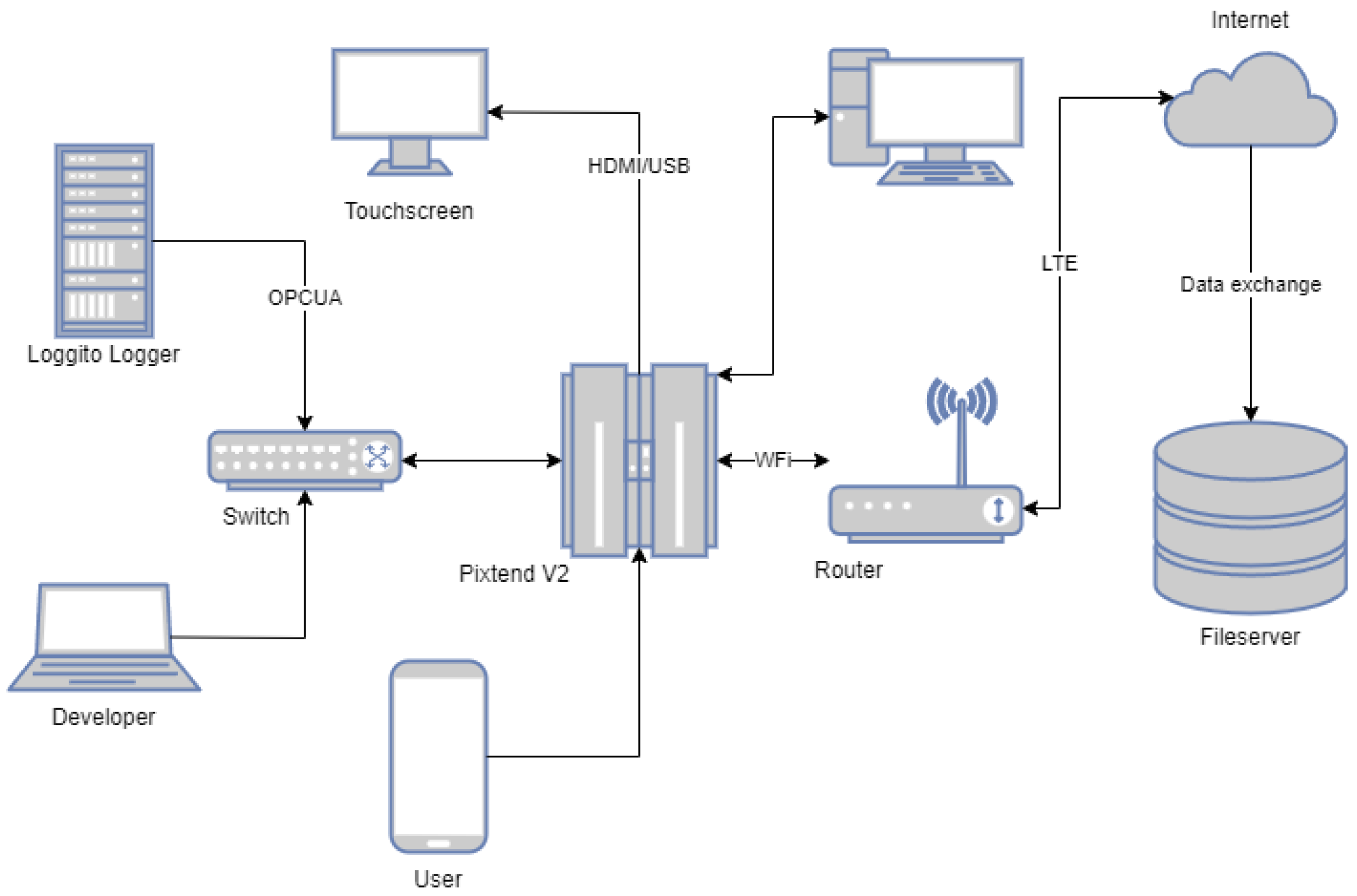
2.5. Data Logging and Database Development

The experimental filter press setup incorporates essential hardware components powered by a 24 V DC input, including a suspension pressure sensor, a flow sensor, and a delphin data logger. The data logger, which operates at a sampling rate of 10 Hz per channel with 24-bit resolution, is suitable for capturing high-resolution data necessary for the analysis of the filtration process. It features an integrated web server and supports the open platform communications unified architecture (OPC UA) protocol, facilitating seamless data transmission and remote access (Figure 4). While the logger enables local data retrieval via USB using proprietary software, it does not inherently support the direct transmission of data to the model environment or provide control functionality for the active components of the filter press. Therefore, an independent control computer was introduced, equipped with a development board containing a quad-core 64-bit ARM Cortex A72 processor. This control system also includes an output module that interfaces with and manages the operation of the active elements in the filter press.
The control computer runs on a 64-bit Ubuntu Linux-based operating system and utilizes an InfluxDB time-series database for local data storage. Node-RED programming facilitates the management of local input and output (I/O) control and orchestrates the data exchange between the control computer and the data logger. Communication between the development board and the data logger is established over an Ethernet connection via the OPC UA protocol, where the data logger functions as the OPC UA server. Once data is transferred to the control system, it undergoes preprocessing, including filtering and analysis, to optimize the data storage load in the database.
The database architecture comprises two interconnected tables: one dedicated to experimental metadata and the other to measured data. The experiment table records user-defined parameters, including the experiment number, number of filter cycles, number of filter chambers, maximum operating pressure, and suspension concentration. These parameters are entered by the user via a graphical interface before initiating each experimental run. The measured data table contains time-stamped data points, such as pressure and flow rate readings, which are linked to the corresponding experiment via the experiment number as a foreign key. This relational structure allows for efficient organization and retrieval of experimental data.
Since InfluxDB utilizes time-based indexing, accurate synchronization between the control computer and the data logger is critical to maintaining data integrity. Initially, the network time protocol (NTP) is employed to synchronize the system clocks. However, given that NTP cannot achieve millisecond-level precision on the data logger, a precision time protocol (PTP) server is subsequently initiated on the control computer. This ensures precise time synchronization between the two systems, which is essential for accurate data logging and analysis.
The system architecture is designed to accommodate various data transmission strategies, depending on the operational context of the filter press. For the prototype system described, the direct transmission of measurement data from the control system to the model cloud server via LTE was selected as the preferred method. This approach facilitates real-time monitoring and data exchange with external databases for further analysis and archiving.

2.6. Neural Network Model

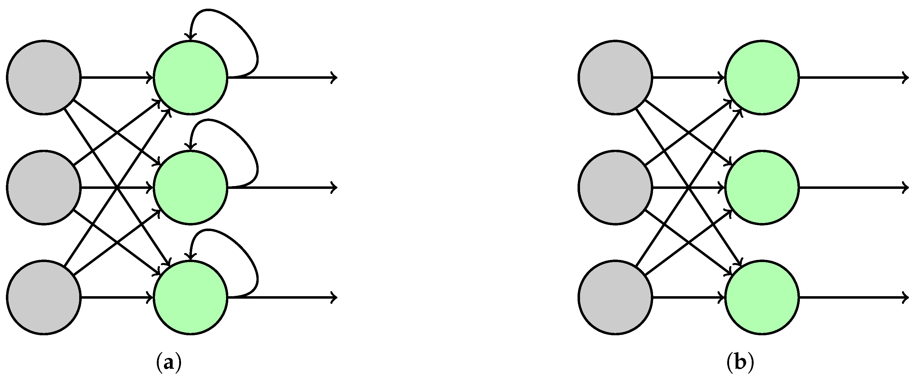
2.6.1. Selection of Neural Network Type

For the model, two NN architectures were considered, the recurrent neural network (RNN) and the feedforward neural network (FFNN), the architecture of which is shown in Figure 5. FFNNs are simple and effective for static data [32]; however, they lack the ability to model temporal dependencies and treat each input independently. RNNs, on the other hand, are explicitly designed to handle sequential data by maintaining an internal state that allows them to retain information from previous time steps [33]. This property makes RNNs particularly well-suited for time-series tasks, such as predicting the pressure and flow rate measurements in a filter press system. In this work, the RNN is implemented using long short-term memory (LSTM) units, which are effective at learning long-term dependencies and mitigating issues such as vanishing gradients, which can occur in standard RNNs. Its downside is that with enough accumulated data, it needs significantly more computational power to train. In this work, both the FFNN and RNN were implemented in order to compare them against each other.
The selection of these two architectures was made to evaluate the trade-off between FFNNs’ simplicity and efficiency for static data, and the temporal modelling capabilities of LSTM-based RNNs. Other architectures, such as gated recurrent unit (GRU) or convolutional neural networks (CNNs), were considered but not selected for this work. GRUs, while simpler than LSTMs, do not capture long-term dependencies as effectively, which can limit their accuracy in applications requiring extended temporal memory. However, their simpler structure, with fewer gates, results in faster training times and reduced computational overhead, making them attractive for scenarios where model efficiency and real-time responsiveness are critical [34]. Despite these advantages, in this work, LSTMs were preferred due to their superior ability to retain information over longer sequences, which is essential for accurately modelling the temporal dynamics of filter press operations. CNNs, which excel in tasks like spatial pattern recognition, are less suited for time-series forecasting tasks where sequential relationships are paramount.

2.6.2. Model Architectures

The FFNN consists of an input layer that accepts a normalized feature vector with five input variables. The model architecture includes two fully connected hidden layers with 64 and 32 neurons, respectively. Each hidden layer utilizes the rectified linear unit (ReLU) activation function to introduce non-linearity and enhance the model’s capability to learn complex relationships. The output layer comprises a single neuron with a linear activation function, suitable for predicting continuous target variables. The FFNN is optimized using the Adam optimizer with a learning rate of 0.001 .
The RNN is configured using an LSTM [35] layer to manage sequential data. The input layer receives sequences of length 10, each consisting of five features per time step. The LSTM layer contains 64 hidden units, enabling the model to capture temporal dependencies effectively. Following the LSTM layer, a fully connected output layer with a single neuron provides the final prediction, using a linear activation function for regression. Similar to the FFNN, the RNN is trained using the Adam optimizer with a learning rate of 0.001 . To facilitate temporal learning, the input data is prepared by generating sequences, allowing the network to leverage internal states for improved prediction accuracy. Data normalization and sequence preparation are essential preprocessing steps that enhance the performance of both models.

2.6.3. Data Preparation

Before training the FFNN or RNN, the input data must undergo preprocessing [36]. The inputs are normalized for both networks using the following standardization formula:
x scaled = x μ σ ,
where μ represents the mean of the input variables and σ denotes their standard deviation.
Although this normalization step is sufficient for training the FFNN, the RNN requires an additional preparation step: sequencing the input variables. This step structures the data into temporal sequences, enabling the RNN to capture patterns over time and develop an internal representation of the expected behaviour of the experiments. This sequencing enhances the RNN’s ability to model temporal dependencies and improves predictive performance.

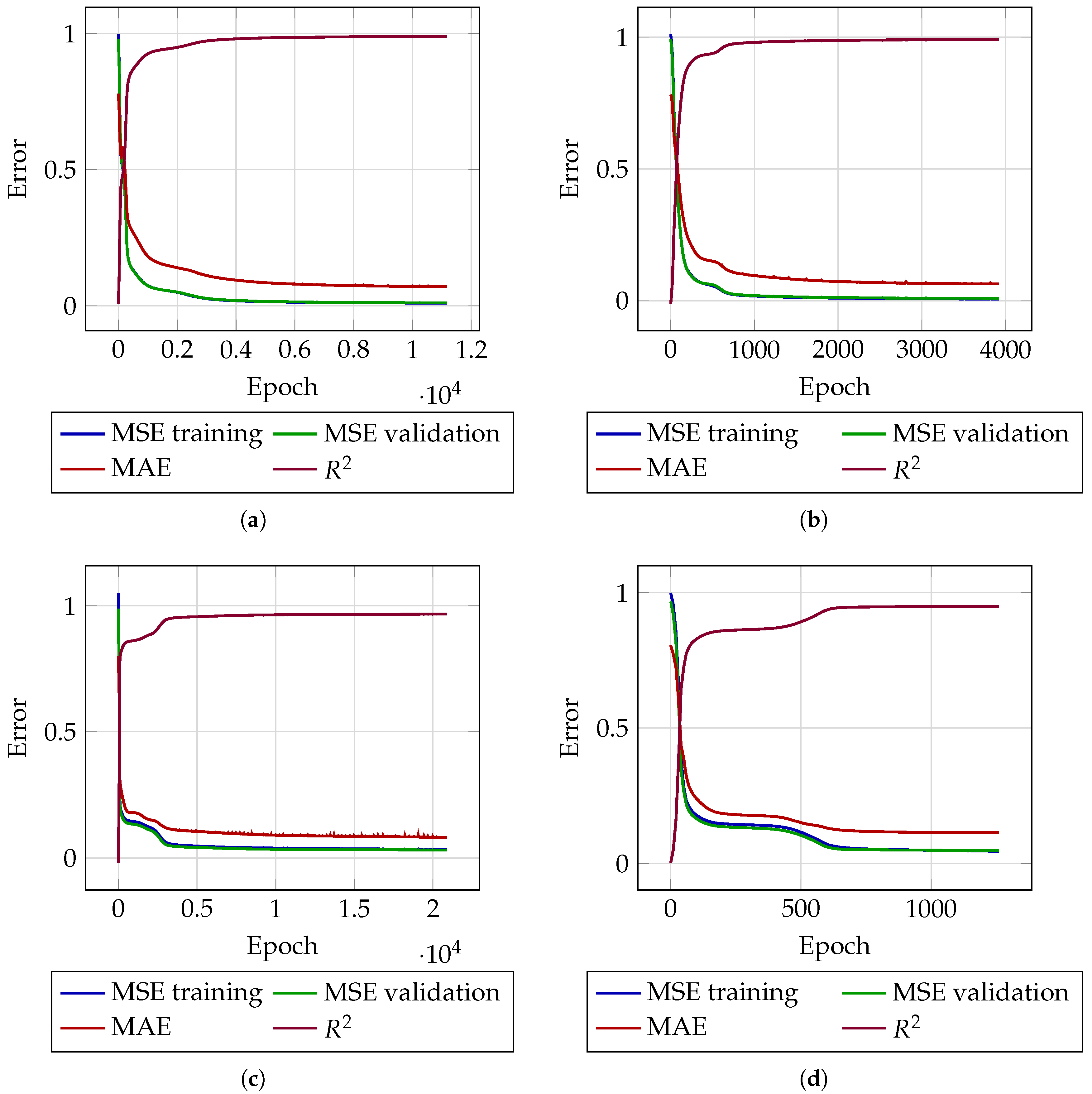
2.6.4. Model Evaluation

The performance of the models was analysed using key metrics such as the MSE, the mean absolute error (MAE), and the coefficient of determination ( R 2 ). These metrics provide complementary insights into the performance of the model. MSE quantifies the average squared differences between true and predicted values, penalizing larger errors more heavily than smaller ones. MAE measures the average absolute difference between true and predicted values, treating all deviations equally, providing a more intuitive interpretation of the average error magnitude compared to MSE. The coefficient of determination ( R 2 ) explains the proportion of variance in the true values captured by the model. The mathematical formulations of these error metrics are provided in Equations (2)–(4):
MSE = 1 n i = 1 n y i y ^ i 2 ,
MAE = 1 n i = 1 n y i y ^ i ,
R 2 = 1 i = 1 n y i y ^ i 2 i = 1 n y i y ¯ 2 ,
where n is the total number of data points, y i represents the true values, and y ^ i denotes the predicted values. For R 2 , y ¯ is the mean of the true values.
These metrics were tracked over the training epochs to evaluate the convergence of the model and to detect potential issues such as overfitting, where the model performs well on training data but poorly on validation data, or underfitting, where the model fails to capture the underlying data patterns.
Figure 6 illustrates the training and validation performance of the FFNN and RNN in predicting both the pressure and the flow rate. As shown in Figure 6b, the RNN model for pressure prediction demonstrates superior convergence and generalization compared to the FFNN model (Figure 6a). The RNN achieves training and validation MSEs of 0.0064 and 0.0093 , respectively. Furthermore, MAE stabilizes at 0.04 , and the R 2 score reaches 0.99 , indicating strong predictive performance. In contrast, FFNN achieves a training MSE of 0.01 and a validation MSE of 0.0108 , with a final R 2 score of 0.98 . Although the FFNN demonstrates reasonable accuracy, the RNN consistently achieves lower errors and faster convergence compared to the FFNN. For flow rate prediction, the FFNN outperforms the RNN in terms of error metrics, achieving training and validation MSEs of 0.031 and 0.034 , respectively, along with an MAE of 0.0823 and an R 2 score of 0.967 . In contrast, the RNN converges to training and validation MSEs of 0.049 and 0.052 , with a final MAE of 0.115 and an R 2 score of 0.9485 . However, Figure 6c reveals that the validation MAE of FFNN exhibits spikes caused by fluctuations in the validation MSE, which increases while the training MSE decreases. This instability suggests overfitting and poorer generalization. In contrast, the RNN model (Figure 6d) achieves a final test MSE of 0.049 , closely aligned with the training MSE, and an MAE of 0.1156 . Unlike the FFNN, the RNN does not exhibit significant fluctuations in validation metrics, indicating better generalization and robustness. Overall, the evaluation suggests that the RNN model is better suited for this task, as it demonstrates superior generalization and stability across both prediction tasks.

3. Results

To evaluate the model, several key points must be addressed. In Figure 7, the true pressure values of an experiment are shown, revealing significant fluctuations in the pressure trend Figure 7a. To fairly assess the prediction error, we first calculated a moving average (MA) and standard deviation (STD) for the experiments, as described by the following equations:
MA ( t ) = 1 n i = t n + 1 t x i ,
STD = 1 n i = t n + 1 t x i MA ( t ) 2 ,
where n is the size of the averaging window, x i represents the data points, and n is the number of data points.
Next, a 90% confidence interval (CI 90 % ) is defined using the calculated STD:
CI 90 = MA ± z · STD ,
where z = 1.645 is the z-score corresponding to the 90% percentile. This interval is used to assess how many predictions fall within the CI 90 % .
By applying these equations to the experiments, an averaged line is obtained with upper and lower bounds, which represent the fluctuations in pressure and flow rate, as shown for the pressure in Figure 7b. This was applied for the flow rate in the same manner.
In addition to MSE and RMSE, the relative L 2 -norm (RL2N) is also used to estimate the percentage error relative to the total magnitude of the experiments. It is defined as
RMSE = 1 n i = 1 n ( y i y ^ i ) 2 ,
RL 2 N = i = 1 n ( y i y ^ i ) 2 i = 1 n y i 2 · 100 ,
where y i represents the true values and y i ^ represents the predicted values. In order to obtain an idea of the deviation of points in regards to the CI 90 % bounds, the L 2 -norm bound (RL2N-B) is introduced and is defined as
RL 2 N - B = i = 1 n e 2 ( x i ) i = 1 n f 2 ( x i ) · 100 ,
e 2 ( x i ) = 0 , if f ^ ( x i ) [ l ( x i ) , u ( x i ) ] , min ( f ^ ( x i ) l ( x i ) ) 2 , ( f ^ ( x i ) u ( x i ) ) 2 , if f ^ ( x i ) [ l ( x i ) , u ( x i ) ] .
where e 2 ( x i ) represents the squared error for the value x i . It is zero if the predicted value f ^ ( x i ) lies within the confidence band [ l ( x i ) , u ( x i ) ] defined by a lower and upper bound. Otherwise, e 2 ( x i ) is computed as the square of the minimum distance between f ^ ( x i ) and the nearest bound of the confidence interval. This formulation ensures that only deviations outside the tolerated range contribute to the total error. The RL2N-B metric thus quantifies how far and how often the prediction violates the expected confidence bounds, rather than simply measuring deviation from a reference value. This is particularly useful in scenarios where predictions are allowed to vary within a known uncertainty band and should only be penalized when they exceed those limits. The denominator i = 1 n f 2 ( x i ) serves as a normalization factor, representing the total squared magnitude of the reference values f ( x i ) . This allows the error to be interpreted as a relative percentage of the baseline signal, enabling fair comparisons across datasets or scales while maintaining a focus on confidence-aware model performance.
Last but not least, the percentage of points inside the CI90% bounds (PIB) is also used for evaluation.
In this section, two experimental datasets are considered: Table 2, which contains experiments used for training and validation (split as 80%/20%), and Table 3, which contains completely unknown experiments, including one with an unknown concentration to the model.

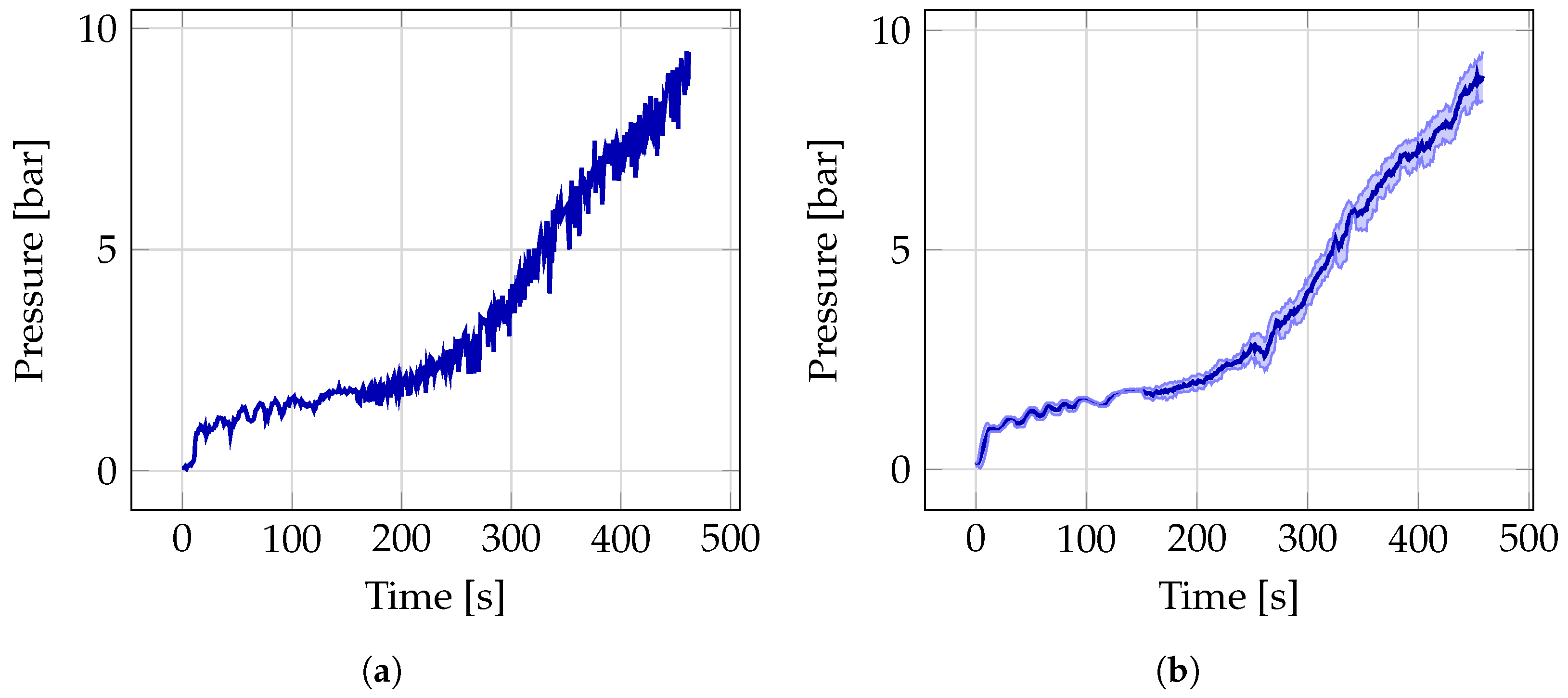
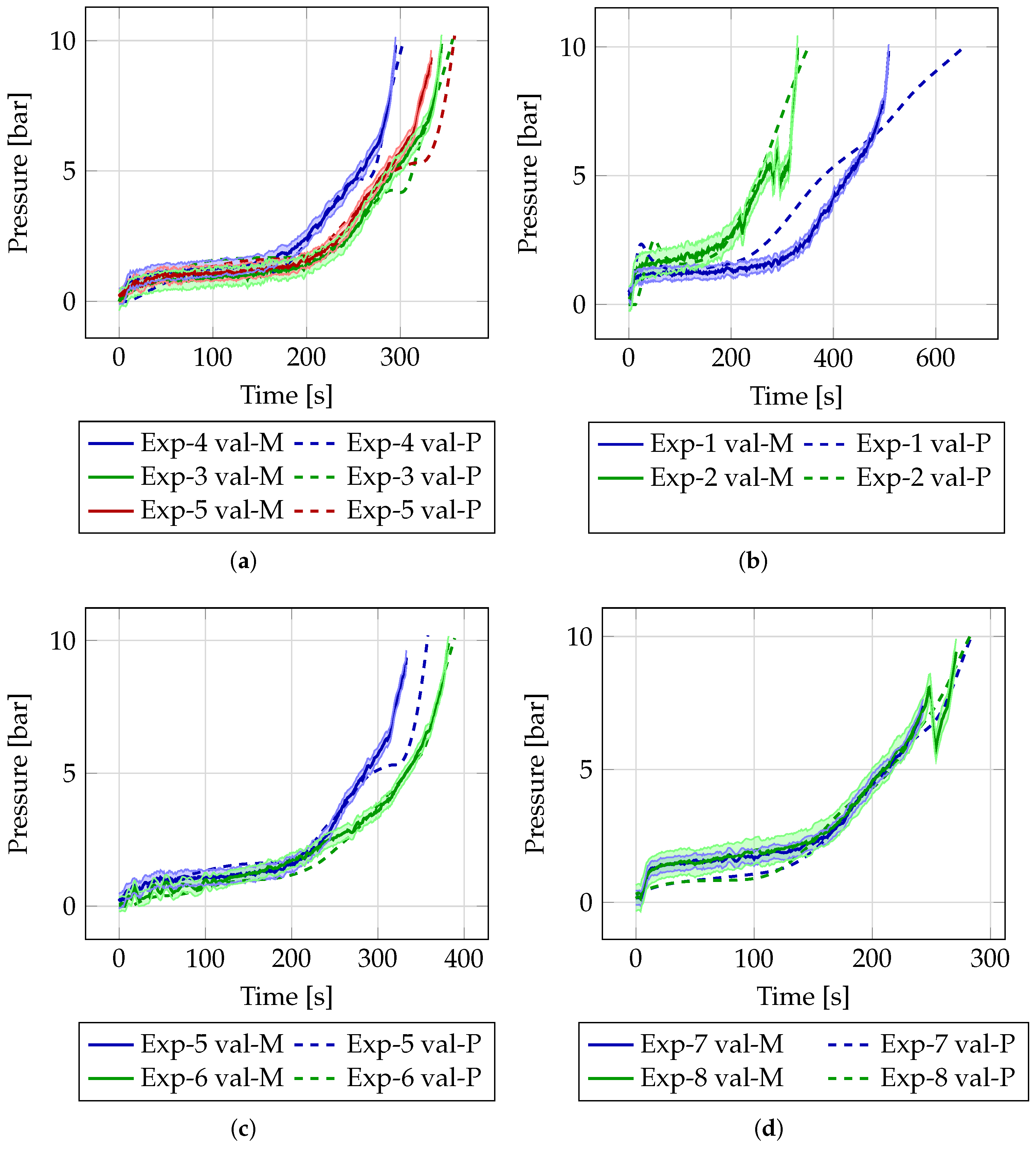
3.1. Pressure Prediction

  • Partially known data
The model demonstrated a strong reliability for pressure prediction in partially known experiments, as illustrated in Figure 8, which compares measured (M) against predicted (P) trends. For experiments with varying filter cycles (Exp-1 to Exp-4, Figure 8a), the predicted pressure profiles closely matched the measured values, with minor deviations observed at higher pressures during later stages. Similarly, experiments with varying concentrations (Exp-5, Exp-3, and Exp-6, Figure 8b) showed high accuracy, although Exp-5 exhibited less precision at maximum pressures due to the absence of training data for a concentration of 6.25 g/L. Figure 8c,d highlight the model’s consistency across different configurations, with slight discrepancies near peak pressures. Quantitative metrics are summarized in Table 4. The errors for partially known experiments ranged from MSE 0.006 to 0.178 , RMSE 0.103 to 0.352 , and RL2N 1.7 % to 9.8 % . The best performance was observed in Exp-5 (RL2N 0.17 % , PIB 97 % ), while Exp-6 had the highest error (RL2N 9.8 % , PIB 64 % ). Overall, the model achieved an average MSE of 0.048 , RMSE of 0.185 , and RL2N of 5 % , with 82 % of the predictions falling within CI90% bounds and minor deviations for the remaining 18 % . The pressure drop around 230 s in Exp-6 (Figure 8d) illustrates the model’s ability to follow expected trends despite limited training data for configurations with three or four plates.
  • Unknown experiments
For unknown experiments, the performance of the model was satisfactory, as shown in Figure 9. The errors for unknown experiments, detailed in Table 5, ranged from MSE 0.100 to 0.838 , RMSE 0.317 to 0.915 , RL2N 9.9 % to 28.2 % , and PIB 64 % to 20 % . Exp-6-val showed the best performance, supported by training data from a similar experiment (Exp-8). In contrast, Exp-1-val exhibited the highest errors due to limited training data at 6.25 g/L and narrow filtration cycle ranges (Figure 9b). Despite these challenges, the model interpolated effectively in experiments with unfamiliar filtration cycles, such as Exp-4-val, achieving good results both qualitatively and quantitatively. Figure 9a highlights deviations at the start and between 260 and 280 s, corresponding to common pressure drops during filtration. Experiments with unknown concentrations (e.g., Exp-7-val and Exp-8-val at 15 g/L, Figure 9c) further demonstrate the generalization capabilities of the model. In general, the mean errors for unknown experiments were MSE 0.403 , RMSE 0.605 , RL2N 18.4 % , and PIB 49.13 % , with minimal deviations outside CI90% bounds (RL2NB 8.2 % ).

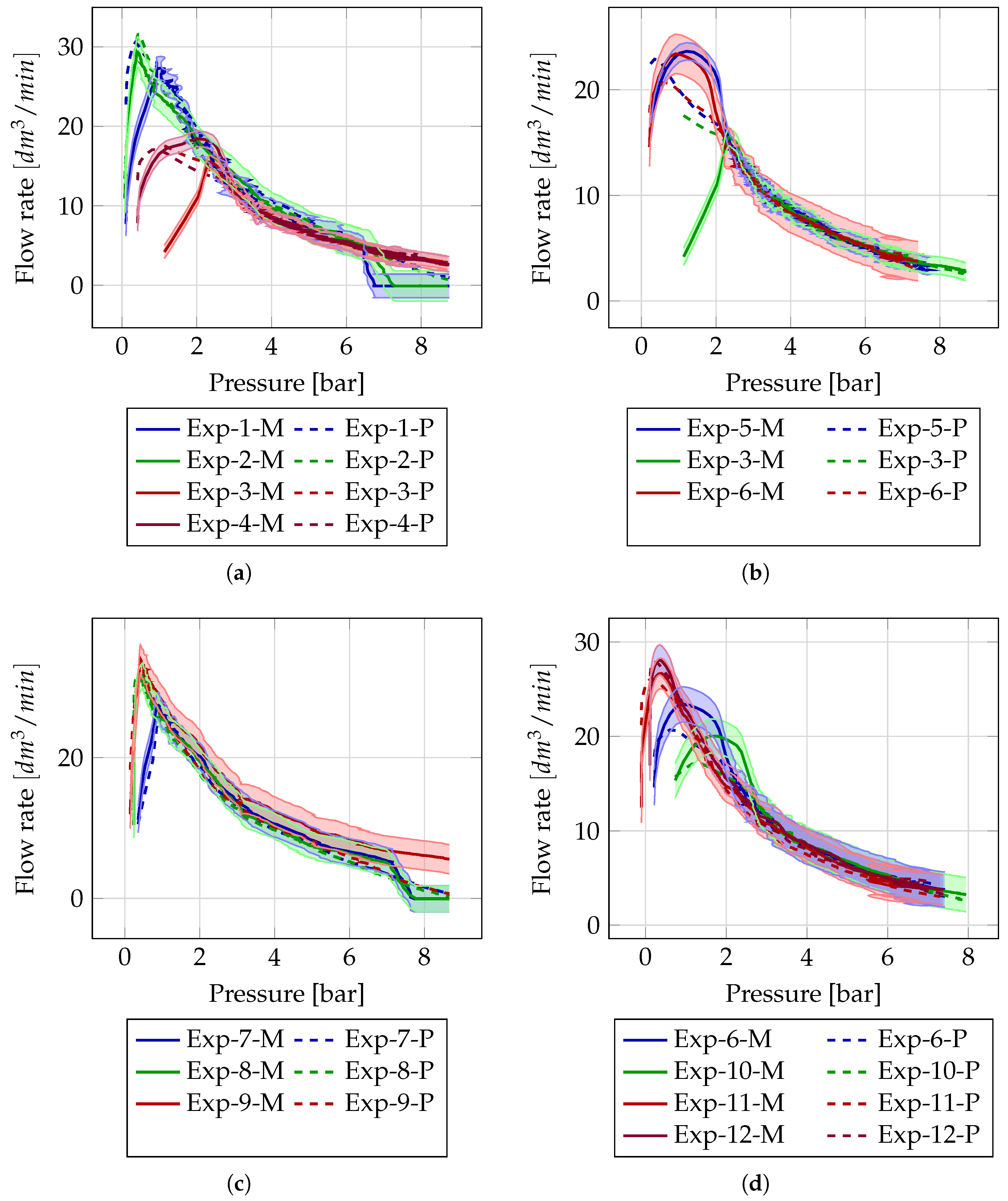
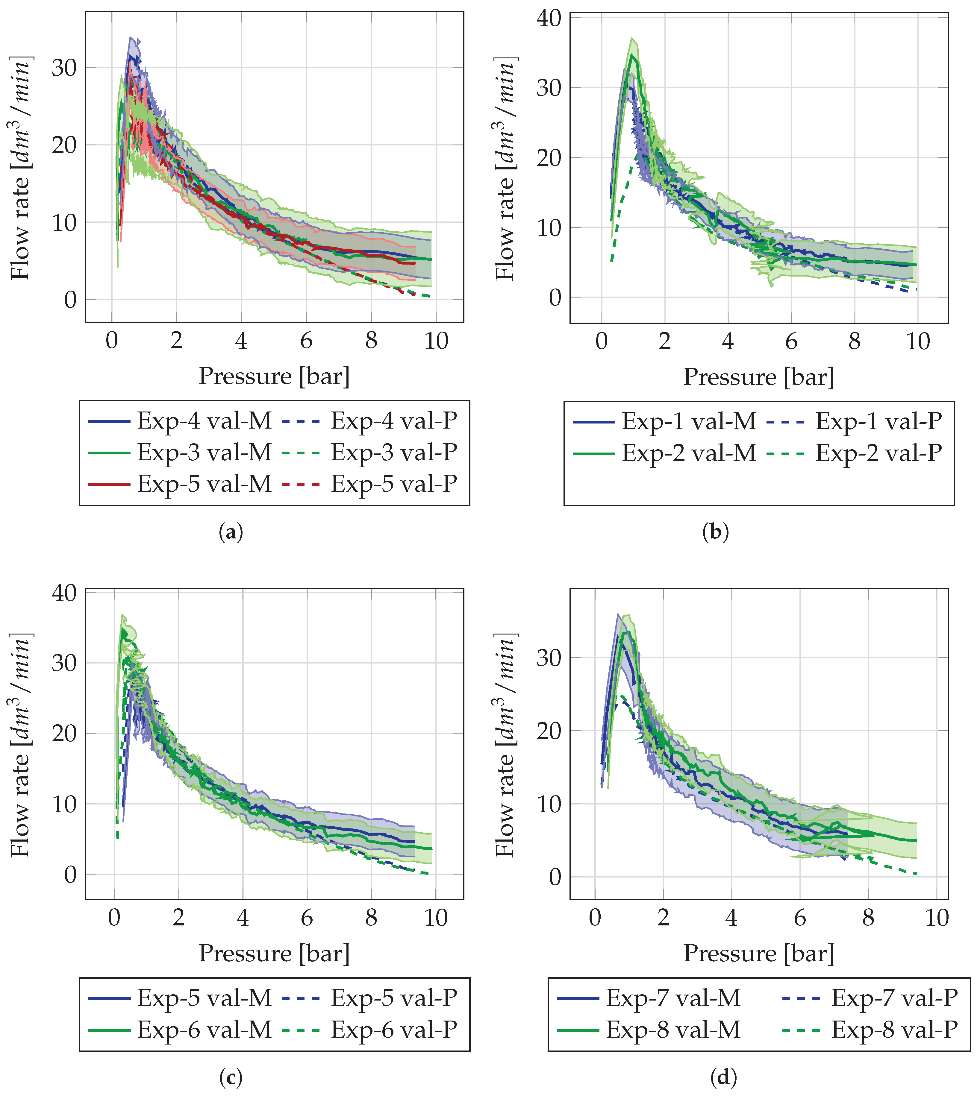
3.2. Flow Rate Prediction

  • Partially known data
The model performed well for flow rate predictions, closely aligning with the experimental setups, as illustrated in Figure 10. The maximum flow rates showed expected trends, such as declines with increasing filter cycles (Figure 10a) and concentrations (Figure 10b). The predictions for varying filter chamber numbers (Figure 10c,d) also matched measured values qualitatively. Quantitative errors for partially known experiments, summarized in Table 4, ranged from MSE 0.339 to 2.150 , RMSE 0.582 to 1.466 , and RL2N 6.2 % to 16.7 % , with 77 % to 89 % of predictions within CI90% bounds. Deviations were linked to specific anomalies. For example, Exp-3 showed initial discrepancies due to clogging, which normalized post-clogging. Exp-5 achieved the best results, closely followed by Exp-12. As seen in Figure 10b, the significant deviation of Exp-5 at the start reflects challenges in initial phase predictions.
  • Unknown experiments
For unknown experiments, the prediction errors, detailed in Table 5, were higher, with averages of MSE 8.229 , RMSE 2.772 , RL2N 15.4 % , and PIB 52.25 % . The worst predictions were in Exp-2-val, where initial trends deviated strongly (Figure 11a,b) due to limited training data for higher flow rates ( 7 dm 3 / min ). In contrast, Exp-6-val performed best, with deviations confined to the end of the filtration process, caused by sensor limitations below 5 dm 3 / min . Experiments at unknown concentrations (15 g/L, Exp-2-val and Exp-3-val) achieved acceptable results, with MSE 4.876 to 9.649 , RMSE 2.208 to 3.106 , RL2N 12.7 % to 17.9 % , and PIB 63 % to 45 % . Figure 11c illustrates the model’s ability to approximate overall trends despite missing knowledge for certain configurations.
Table 4. Prediction errors for experiments in the validation and training sets, evaluated for both pressure and flow rate. Metrics include MSE (mean squared error), RMSE (root mean squared error), RL2N (relative L 2 norm error), RL2N-B (relative L 2 norm error with respect to CI90 bounds), and PIB (percentage of points within bounds).
Experiment Pressure Flow Rate
MSE RMSE RL2N
[%]
RL2N-B
[%]
PIB [%] MSE RMSE RL2N
[%]
RL2N-B
[%]
PIB [%]
10.0410.2024.60.5964.9552.22613.45.350
20.0110.1032.60.1983.8681.9679.82.364
30.0410.2024.11.3742.1501.46616.710.677
40.0360.1903.70.9750.4680.6848.43.469
50.0060.0751.70.3970.3390.5826.22.689
60.1780.4219.84.7641.4131.18910.23.662
70.0130.1142.70.2982.9051.7049.23.360
80.0450.2115.82.4763.9531.9889.14.991
90.0080.0882.20.01003.9341.9838.51.677
100.0380.1964.10.5860.9840.9929.92.766
110.0660.2576.72.3751.0821.0407.03.193
120.1240.3529.24.8710.9140.9566.13.198
Mean0.0480.1855.01.8822.5791.5459.33.774
Table 5. Prediction errors for experiments completely unknown to the model, evaluated for both pressure and flow rate. Metrics include MSE (mean squared error), RMSE (root mean squared error), RL2N (relative L 2 norm error), RL2N-B (relative L 2 norm error with respect to CI90 bounds), and PIB (percentage of points within bounds).
Experiment Pressure Flow Rate
MSE RMSE RL2N
[%]
RL2N-B
[%]
PIB [%] MSE RMSE RL2N
[%]
RL2N-B
[%]
PIB [%]
1-val0.8380.91528.215.820.0010.2813.20618.06.750.00
2-val0.7090.84224.211.946.0012.5933.54920.97.835.00
3-val0.2500.50016.15.947.0013.8453.72120.95.155.00
4-val0.1710.41413.34.354.001.7371.3186.61.384.00
5-val0.4880.69922.313.152.006.3232.51513.53.737.00
6-val0.1000.3179.92.964.006.5312.55512.65.749.00
7-val0.2730.52316.87.154.004.8762.20812.72.863.00
8-val0.3970.63016.44.856.009.6493.10617.95.445.00
Mean0.4030.60518.48.249.138.2292.77215.44.852.25

3.3. Current Limitations and Future Work

While the presented approach demonstrates strong performance and accurate predictions within the tested setup, several limitations remain that offer opportunities for further enhancement of the model’s robustness and generalizability.
  • Material specificity: As described in Section 2.1, all experiments were carried out using a single suspension, perlite, to ensure consistent results. However, other suspensions such as kieselgur exhibit significantly different behaviours due to their high porosity and fluid retention characteristics. This may affect the direct applicability of the current model to a broader range of materials.
  • Limited scalability: The experiments were performed using a chamber filter press with a plate size of 300 mm. While the current model has shown that it can adapt to different configurations if such setups are included during training, its ability to generalize to presses of different sizes remains dependent on the diversity of the training data. Without sufficient variation, scaling the model to untested press sizes or configurations may be less reliable.
  • Hardware dependency: The predictive accuracy of the model is influenced by the mechanical state of the system. Irregularities, such as inefficiencies in the membrane pump, leaks, or hardware degradation, can affect performance and introduce noise into the training data. If such anomalies remain undetected, they could gradually influence model performance.
To address these limitations, future work will focus on expanding the dataset to include a wider variety of suspensions, operating conditions, and press configurations. Thanks to the installed sensor setup from Section 2.5, the experimental data is continuously collected and stored in a central database, allowing automatic model updates as new operational scenarios arise. Incorporating anomaly detection and additional sensor types can further improve resilience to hardware-related issues. Ultimately, a more diverse and representative dataset is expected to not only improve model accuracy but also enhance its ability to generalize to unseen scenarios. In addition, we will explore whether it is possible to normalize relevant features and upscale the existing model to different filter press sizes without requiring retraining from scratch. Furthermore, the use of physics-informed neural networks incorporating domain equations such as the Darcy law will be explored, particularly for modelling porous materials such as kieselgur, where fluid–solid interactions play a more dominant role.

4. Conclusions

This study introduces a novel ML-based DT framework to sustainably predict key operational parameters of chamber filter presses, specifically pressure and flow rates. The framework was evaluated using two datasets: one for training and validation, and another with unknown experimental configurations.
Summary of evaluation:
  • Pressure prediction (training and validation): Overall, MSE was 0.048 , RMSE was 0.185 and RL2N was 5.0 % . Deviation from the CI90% bounds was 1.8 % .
  • Flow rate prediction (training and validation): Overall, MSE was 2.579 , RMSE was 1.545 and RL2N was 9.3 % . Deviation from the CI90% bounds was 3.7 % .
  • Pressure prediction (unknown data): Overall MSE was 0.403 , RMSE was 0.605 and RL2N was 18.4 % . Deviation from the CI90% bounds was 8.2 % .
  • Flow rate prediction (unknown data): Overall MSE was 8.229 , RMSE was 2.772 , and RL2N was 15.4 % . Deviation outside CI90% bounds was 4.8 % .
The comparison of RMSE and MSE values suggests fewer significant errors and more frequent small deviations in flow rate predictions. Furthermore, the model’s ability to interpolate between known configurations (e.g., 12.5 g/L and 25 g/L) to approximate unknown configurations (e.g., 15 g/L) highlights its practical utility, even in cases with limited training data. However, errors for specific configurations, such as 6.25 g/L, indicate that broader training datasets should be considered in future studies to further enhance performance in edge cases.
This DT framework, which integrates real-time data and predictive analytics, represents a significant step forward in optimizing chamber filter press operations. By accurately forecasting pressure and flow rates and estimating the lifespan of the filter medium, the system enables more efficient process control, reduces downtime, enhances resource utilization, and supports sustainable practices. The model can be adopted by operators in industrial filtration settings such as mining, wastewater treatment, and pharmaceuticals, where data-driven optimization is essential. It is particularly suited for applications involving repetitive, measurable processes that benefit from predictive maintenance and efficiency improvements. Future work will focus on expanding the diversity of operational scenarios, improving prediction accuracy for sparsely trained configurations, and further refining the model’s adaptability to evolving industrial conditions.

Author Contributions

Conceptualization, D.T.; methodology, D.T.; software, D.T.; validation, D.T. and S.S.; formal analysis, D.T. and S.S.; investigation, D.T.; resources, M.J.K. and T.W.-C.; data curation, D.T.; writing—original draft preparation, D.T.; writing—review and editing, S.S. and M.J.K.; supervision, M.J.K.; project administration, M.J.K.; funding acquisition, M.J.K. and T.W.-C. All authors have read and agreed to the published version of the manuscript.

Funding

The current research is part of the Invest BW project BW1_0027/01 “Filt-AR: Entwicklung einer neuen Filt-AR-Filterpresse mit wissensbasierter Regelung anhand eines digitalen Zwillings und Augmented Reality-Visualisierung”.

Institutional Review Board Statement

Not applicable.

Informed Consent Statement

Not applicable.

Data Availability Statement

Data is contained within the article.

Conflicts of Interest

Author T.W.-C. was employed by the company Simex Filterpressen und Wassertechnik GmbH & Co. KG. The remaining authors declare that the research was conducted in the absence of any commercial or financial relationships that could be construed as a potential conflict of interest.

Abbreviations

The following abbreviations are used in this manuscript:
AIartificial intelligence
ARaugmented reality
CI9090% confidence interval
CFDcomputational fluid dynamics
CNNconvolutional neural network
DTdigital twin
FFNNfeedforward neural network
GRUgated recurrent unit
LBMLattice Boltzmann method
LSTMlong short-term memory
MAmoving average
MAEmean absolute error
Mmeasured
MSEmean square error
MLmachine learning
NNneural network
NTPnetwork time protocol
OPC UAopen platform communications unified architecture
Ppredicted
PIBpoint inside bounds
PTPprecision time protocol
ReLUrectified linear unit
RL2Nrelative L 2 -norm
RL2N-Brelative L 2 -norm bounds
RMSEroot mean square error
RNNrecurrent neural network
STDstandard deviation

References

  1. Garner, R.; Naidu, T.; Saavedra, C.; Matamoros, P.; Lacroix, E. Water Management in Mining: A Selection of Case Studies; International Council on Mining & Metals: London, UK, 2012. [Google Scholar]
  2. Gunson, A.; Klein, B.; Veiga, M.; Dunbar, S. Reducing mine water requirements. J. Clean. Prod. 2012, 21, 71–82. [Google Scholar] [CrossRef]
  3. Baker, E. Mine Tailings Storage: Safety Is No Accident; GRID-Arendal: Arendal, Norway, 2017. [Google Scholar]
  4. Matschullat, J.; Gutzmer, J. Mining and Its Environmental Impacts. In Encyclopedia of Sustainability Science and Technology; Springer: New York, NY, USA, 2012; pp. 6633–6645. [Google Scholar] [CrossRef]
  5. Tran, T.; Truong, T.; Tran, T.; Hài, N.; Dao, Q. An overview of the application of machine learning in predictive maintenance. Petrovietnam J. 2021, 10, 47–61. [Google Scholar] [CrossRef]
  6. McCoy, J.; Auret, L. Machine learning applications in minerals processing: A review. Miner. Eng. 2019, 132, 95–109. [Google Scholar] [CrossRef]
  7. Anagnostopoulos, I.; Chatzilygeroudis, K.; Maragos, P. A Prototype Implementation of Factory Monitoring Using VR and AR Technologies. arXiv 2023, arXiv:2306.09692. [Google Scholar]
  8. Alpha Wastewater. Wastewater Treatment and Augmented Reality: Visualizing Processes and Optimizing Operations. 2023. Available online: https://www.alphawastewater.com/wastewater-treatment-and-augmented-reality-visualizing-processes-and-optimizing-operations/?utm_source=chatgpt.com (accessed on 16 April 2025).
  9. Alatawi, H.; Albalawi, N.; Shahata, G.; Aljohani, K.; Alhakamy, A.; Tuceryan, M. An AR-Assisted Deep Reinforcement Learning-Based Model for Industrial Training and Maintenance. Sensors 2023, 23, 6024. [Google Scholar] [CrossRef]
  10. Landman, K.A.; White, L.R. Predicting filtration time and maximizing throughput in a pressure filter. AIChE J. 1997, 43, 3147–3160. [Google Scholar] [CrossRef]
  11. Puig-Bargués, J.; Duran-Ros, M.; Arbat, G.; Barragán, J.; Ramírez de Cartagena, F. Prediction by neural networks of filtered volume and outlet parameters in micro-irrigation sand filters using effluents. Biosyst. Eng. 2012, 111, 126–132. [Google Scholar] [CrossRef]
  12. Hawari, A.H.; Alnahhal, W. Predicting the performance of multi-media filters using artificial neural networks. Water Sci. Technol. 2016, 74, 2225–2233. [Google Scholar] [CrossRef] [PubMed]
  13. Griffiths, K.; Andrews, R. Application of artificial neural networks for filtration optimization. J. Environ. Eng. 2011, 137, 1040–1047. [Google Scholar] [CrossRef]
  14. Khan, W.A.; Chung, S.H.; Awan, M.U.; Wen, X. Machine learning facilitated business intelligence (Part I): Neural networks learning algorithms and applications. Ind. Manag. Data Syst. 2020, 120, 657–698. [Google Scholar] [CrossRef]
  15. Khan, W.A.; Chung, S.H.; Eltoukhy, A.E.; Khurshid, F. A novel parallel series data-driven model for IATA-coded flight delays prediction and features analysis. J. Air Transp. Manag. 2024, 114, 102488. [Google Scholar] [CrossRef]
  16. Spielman, L.; Goren, S.L. Model for predicting pressure drop and filtration efficiency in fibrous media. Environ. Sci. Technol. 1968, 2, 279–287. [Google Scholar] [CrossRef]
  17. Krause, M.J.; Kummerländer, A.; Avis, S.J.; Kusumaatmaja, H.; Dapelo, D.; Klemens, F.; Gaedtke, M.; Hafen, N.; Mink, A.; Trunk, R.; et al. OpenLB—Open source lattice Boltzmann code. Comput. Math. Appl. 2021, 81, 258–288. [Google Scholar] [CrossRef]
  18. Krause, M.J.; Klemens, F.; Henn, T.; Trunk, R.; Nirschl, H. Particle flow simulations with homogenised lattice Boltzmann methods. Particuology 2017, 34, 1–13. [Google Scholar] [CrossRef]
  19. Trunk, R.; Bretl, C.; Thäter, G.; Nirschl, H.; Dorn, M.; Krause, M.J. A Study on Shape-Dependent Settling of Single Particles with Equal Volume Using Surface Resolved Simulations. Computation 2021, 9, 40. [Google Scholar] [CrossRef]
  20. Stipić, D.; Budinski, L.; Fabian, J. Sediment transport and morphological changes in shallow flows modelled with the lattice Boltzmann method. J. Hydrol. 2022, 606, 127472. [Google Scholar] [CrossRef]
  21. Hafen, N.; Dittler, A.; Krause, M.J. Simulation of particulate matter structure detachment from surfaces of wall-flow filters applying lattice Boltzmann methods. Comput. Fluids 2022, 239, 105381. [Google Scholar] [CrossRef]
  22. Zhang, X.; Zhang, Z.; Zhang, Z.; Zhang, X. Lattice Boltzmann modeling and analysis of ceramic filtration with different pore structures. J. Taiwan Inst. Chem. Eng. 2022, 132, 104–113. [Google Scholar] [CrossRef]
  23. Haussmann, M.; Ries, F.; Jeppener-Haltenhoff, J.B.; Li, Y.; Schmidt, M.; Welch, C.; Illmann, L.; Böhm, B.; Nirschl, H.; Krause, M.J.; et al. Evaluation of a Near-Wall-Modeled Large Eddy Lattice Boltzmann Method for the Analysis of Complex Flows Relevant to IC Engines. Computation 2020, 8, 43. [Google Scholar] [CrossRef]
  24. Wichmann, K.R. Evaluation and Development of High Performance CFD Techniques with Focus on Practice-Oriented Metrics. Ph.D. Thesis, Technische Universität München, Munich, Germany, 2014. [Google Scholar]
  25. Callé, S.; Bémer, D.; Thomas, D.; Contal, P.; Leclerc, D. Changes in the performances of filter media during clogging and cleaning cycles. Ann. Occup. Hyg. 2001, 45, 115–121. [Google Scholar] [CrossRef]
  26. Kandra, H.S.; McCarthy, D.; Fletcher, T.D.; Deletic, A. Assessment of clogging phenomena in granular filter media used for stormwater treatment. J. Hydrol. 2014, 512, 518–527. [Google Scholar] [CrossRef]
  27. Kehat, E.; Lin, A.; Kaplan, A. Clogging of filter media. Ind. Eng. Chem. Process. Des. Dev. 1967, 6, 48–55. [Google Scholar] [CrossRef]
  28. Fränkle, B.; Morsch, P.; Nirschl, H. Regeneration assessments of filter fabrics of filter presses in the mining sector. Miner. Eng. 2021, 168, 106922. [Google Scholar] [CrossRef]
  29. Callé, S.; Contal, P.; Thomas, D.; Bémer, D.; Leclerc, D. Description of the clogging and cleaning cycles of filter media. Powder Technol. 2002, 123, 40–52. [Google Scholar] [CrossRef]
  30. Lyu, Z. (Ed.) Handbook of Digital Twins, 1st ed.; CRC Press: Boca Raton, FL, USA; Routledge: London, UK, 2024. [Google Scholar] [CrossRef]
  31. Teutscher, D.; Weckerle, T.; Öz, Ö.F.; Krause, M.J. Interactive Scientific Visualization of Fluid Flow Simulation Data Using AR Technology-Open-Source Library OpenVisFlow. Multimodal Technol. Interact. 2022, 6, 81. [Google Scholar] [CrossRef]
  32. Sandberg, I.W.; Lo, J.T.; Fancourt, C.L.; Principe, J.C.; Katagiri, S.; Haykin, S. Nonlinear Dynamical Systems: Feedforward Neural Network Perspectives; John Wiley & Sons: Hoboken, NJ, USA, 2001; Volume 21. [Google Scholar]
  33. Sherstinsky, A. Fundamentals of Recurrent Neural Network (RNN) and Long Short-Term Memory (LSTM) network. Phys. D Nonlinear Phenom. 2020, 404, 132306. [Google Scholar] [CrossRef]
  34. Waqas, M.; Humphries, U.W. A critical review of RNN and LSTM variants in hydrological time series predictions. MethodsX 2024, 13, 102946. [Google Scholar] [CrossRef]
  35. Mienye, I.D.; Swart, T.G.; Obaido, G. Recurrent Neural Networks: A Comprehensive Review of Architectures, Variants, and Applications. Information 2024, 15, 517. [Google Scholar] [CrossRef]
  36. McClarren, R. Feed-Forward Neural Networks; Springer International Publishing: Berlin/Heidelberg, Germany, 2021; pp. 119–148. [Google Scholar] [CrossRef]
Figure 1. (a) Full view of the chamber filter press, showing the filter press unit with multiple filter chambers. The number of chambers directly correlates with the volume of suspension that can be filtered in a single cycle. (b) Close-up view of an individual filter chamber, highlighting the filter cloth (black) inside. Each chamber is where the filtration process occurs, with the slurry being pressurized, allowing the liquid to pass through the cloth while retaining the solids as filter cakes.
Applsci 15 04933 g001
Figure 2. Architecture of the DT framework for a chamber filter press, illustrating the communication flow between the filter press, real-time measuring techniques, the central database, the predictive model, and the operator.
Applsci 15 04933 g002
Figure 3. Integration of augmented reality (AR) with the digital twin (DT) framework [31]. This figure shows a virtual 3D model of a chamber filter press overlaid onto its physical counterpart using AR. At the current stage, the AR system primarily supports visualization of the geometry and structure of the filter press. It can assist operators by highlighting specific components—such as individual filter chambers—and providing interactive maintenance instructions, for example, indicating how to access or remove parts. This lays the foundation for future functionality, such as real-time diagnostics or condition monitoring.
Applsci 15 04933 g003
Figure 4. Schematic overview of the data acquisition and communication architecture for the chamber filter press system. The setup includes a Delphin data logger connected to sensors for pressure and flow rate measurement, which communicates with a control unit via OPC UA. The control system, represented by a PiXtend V2 board, interfaces with peripheral devices such as a touchscreen and user input terminals through HDMI/USB. Data transfer and remote monitoring are facilitated through a router, enabling Wi-Fi connectivity and LTE-based transmission to a file server for storage and further analysis. Developers and operators can access the system remotely or locally for control and data export.
Applsci 15 04933 g004
Figure 5. Comparison of RNN (a) and FFNN (b). Gray nodes represent input neurons, and green nodes represent hidden neurons in both architectures. In (a), the RNN includes feedback loops, represented by the arrows looping back from the hidden neurons to themselves, enabling the processing of sequential data and temporal dependencies. The arrows pointing to the right indicate information flow to the output. In (b), the FFNN consists of direct connections between neurons, without feedback loops, illustrating a simpler network structure designed for static data processing.
Applsci 15 04933 g005
Figure 6. Error metrics MSE, MAE, and R 2 for training and validation data during training of pressure and flow models. Figure (a,b) represent FFNN and RNN models for pressure prediction, respectively, while (c,d) depict FFNN and RNN models for flow prediction.
Applsci 15 04933 g006
Figure 7. Depicted is the RAW data of a pressure trend in (a) and the MA pressure trend in (b) with CI90% bounds.
Applsci 15 04933 g007
Figure 8. Comparison of measured (M) and predicted (P) pressure values for the experiments from the Table 2. (a) shows the increase in operation time with higher cycle number. (b) shows the increase in operation time with different concentrations and similar filter cycle. (c,d) show the operational time with different numbers of filter chambers.
Applsci 15 04933 g008
Figure 9. Comparison of measured (M) and predicted (P) pressure values for the experiments listed in Table 3. (a) illustrates the increase in operational time with a higher number of filter cycles. (b) depicts the increase in operational time for different concentrations while maintaining similar filter cycles. (c) demonstrates the variation in operational time with differing numbers of filter chambers. (d) presents the prediction for an unknown concentration of 15 g/L.
Applsci 15 04933 g009
Figure 10. Comparison of measured (M) and predicted (P) flow rate for the experiments from Table 2. (a) shows the reduction in the flow rate with higher cycle numbers over the pressure. (b) shows the reduction in the flow rate with different concentrations and similar filter cycles over the pressure. (c,d) shows the flow rate with different numbers of filter chambers over the pressure.
Applsci 15 04933 g010
Figure 11. Comparison of measured (M) and predicted (P) flow rate for the experiments listed in Table 3. (a) illustrates the reduction in flow rate with a higher number of filter cycles. (b) shows the reduction in the flow rate with different concentrations and similar filter cycles over the pressure. (c) shows the increase in flow rate with different numbers of filter chambers. (d) presents the prediction of the flow rate for an unknown concentration of 15 g/L.
Applsci 15 04933 g011
Table 1. Available training and validation data from experiments.
Concentration [g/L]Filter Plate NumberEnd Pressure [bar]CyclesFrequency
6.2522.0341
6.2524.0321
6.2525.0311
6.2526.0301
6.2528.0291
12.5011041
12.50210.02, 4, 5, 6, 7, 14,
23, 35, 36
9
12.5027.051
12.5028.061
12.5020.211
12.5020.510,112
12.5020.712,132
12.503101,2,33
25.00210.0241
25.0025.0181
25.0026.0191
25.0027.0201
25.0028.0211
25.0029.0221
25.00210.0231
25.00310.0251
25.00410.0261
Table 2. Experiment data with diverse configurations and filter cycles. The experiment is partially known to the model since it was split into 80 % training and 20 % validation data.
ExperimentConcentration [g/L]Filter Plate NumberEnd Pressure (bar)Cycles
112.52102
212.52107
312.521035
412.521036
56.252829
62521023
712.51104
812.53102
912.52105
102511024
112531025
122541026
Table 3. Experiment data with diverse configurations and filter cycles. The experiments are completely unknown to the model.
ExperimentConcentration [g/L]Filter Plate NumberEnd Pressure (bar)Cycles
1 val6.2521024
2 val12.521030
3 val12.521011
4 val12.521010
5 val12.52109
6 val12.53106
7 val152107
8 val152108
Disclaimer/Publisher’s Note: The statements, opinions and data contained in all publications are solely those of the individual author(s) and contributor(s) and not of MDPI and/or the editor(s). MDPI and/or the editor(s) disclaim responsibility for any injury to people or property resulting from any ideas, methods, instructions or products referred to in the content.

