RoPT: Route-Planning Model with Transformer

Abstract

With the increasing aggravations of urban traffic jams, intelligent route planning to reduce traffic time is becoming increasingly critical for drivers. However, traditional route-planning methods, such as graph search and Recurrent Neural Network (RNN)-based methods, struggle to capture the complex dynamics of road networks. Specifically in A*-type methods, routes should be searched instantly on the whole graph for the sake of dynamic changes in edge time consumption. As for RNN-based methods, their shortcomings in capturing long-distance sequence dependencies makes them unsuitable for route planning in metropolises with long routes. Therefore, to better adapt to the complexity of urban traffic, in this paper, an innovative route-planning model called Route Planning with Transformer (RoPT) is proposed. This model is based on the fusion of Graph Convolutional Networks (GCNs) and a Transformer, which uses GCNs for capturing complex spatial dependencies between the current intersection and the destination in a road network. Depending on the self-attention mechanism of the Transformer, the long-distance temporal dependencies between intersections could also be captured effectively. With comprehensive experiments on two real-world traffic datasets, the Porto dataset and the Chengdu dataset, it is demonstrated that RoPT outperforms the best methods, to the best of our knowledge. Moreover, the latent features learned from RoPT are more interpretable.

1. Introduction

With the rapid development of urbanization, urban traffic jams become increasingly prominent. To reduce computing time and enhance the life quality of residents, it is more urgent to accurately predict urban traffic information such as traffic volume, vehicle speed, and traffic time, and process it in a timely fashion. Thus, with its important applications in the navigation of taxis, shared bicycles, and takeouts, as well as in other fields, route planning attracts more and more attentions of researchers.

The role of route planning is to predict the most likely path in a road network between the given source node and the destination node. In the traditional research of route planning, graph search algorithms are focused on finding the path with the smallest cost in a given road network, according to the weights of the edges connecting the nodes, such as distance, traffic time, etc. However, with the increasing traffic, more attention is paid to traffic time, and the weights of the edges are changing dynamically, which makes them ineffective when capturing complex spatial–temporal structures and the dynamics of road networks. Naturally, these algorithms are unable to adapt to even more complicated circumstances, such as accidents that happened in urban traffic. In our analysis of taxi routes from Porto, it could be seen that, in actual routes, the appearance probabilities of transportation hubs and main roads are much larger than those planned with Dijkstra. This phenomenon probably comes from the fact that travel time in the narrow streets of the old town of Porto is much longer, so the drivers choose to take a detour.

To make route-planning prediction more accurate and comprehensive, machine learning is introduced to mine the complex dynamics of traffic. (1) As a road network is essentially a graph, and the features of traffic are typically temporal, Graph Neural Networks (GNNs) and its variants, for processing complex spatial topologies, and Recurrent Neural Networks (RNNs) and its variants, for obtaining temporal patterns, are used in route planning. Research includes CSSRNN [1], NEUROMLR [2], and GETNext [3]. (2) Noting that RNN methods are not suitable for learning long-term dependencies, researchers have recently begun to combine GNNs and a Transformer for molecular property prediction and image classification [4,5]. In these studies, GNNs were used to understand the local short-term dependencies, and the Transformer was used to learn the global long-term dependencies. Moreover, the combinations of GNNs and a Transformer, such as Graphormer [6] and GEIT [7], where graph features are encoded and inputted into the Transformer, is needed for route planning. However, these methods both have their shortcomings in traffic route planning. In the former, the computed graph features are static, which does not closely align with the requirements of prediction tasks. In the latter, a route is planned with a Divide-and-Conquer framework in order to recursively identify an intermediate road section to divide a route into two sub-routes for planning. Thus, destination, a key factor, is omitted when planning sub-routes. (3) As we know, when a city becomes bigger, the number of intermediate road sections of a long route also becomes bigger. Then, the planning performance is degraded due to the sparsity of intermediate road sections. Thus, an alternative approach is considered for predicting the next road sections from a source node, step by step. However, in this kind of approach, the prediction results gained from the current route are often influenced by the destinations frequently visited by the public, which are not the true destinations. Thus, the planning results should be adjusted using the results predicted based on the true destination.

In summary, in this paper, an innovative route-planning model, which is based on the combination of a GCN and Transformer for metropolises, RoPT, is proposed. In this model, multiple layers of GCNs are stacked together to capture the dependencies between different sections of a road network. Then, a self-attention mechanism of the Transformer is used to capture the long-term dependencies in sequences. In the end, due to the importance of the destination in guiding the direction of a route, features of the destination learned from the GCN are used to adjust the next road section.

The main contributions of this paper are summarized as follows:

(1) The RoPT is proposed, combining a multi-layer GCN module and Transformer module to better capture the complex dependencies between road sections, including spatial and temporal dependencies.

(2) A new method of destination embedding is proposed to add the influence of destination features and current route features into the transfer probability, to improve the prediction performance.

(3) Comprehensive experiments are conducted on two publicly available traffic datasets, whose results show that RoPT outperforms all of the baselines, to the best of our knowledge.

The rest of this paper is organized as follows. In Section 2, related works on route planning are discussed. In Section 3, a preliminary definition of route planning is presented. The framework and evaluations of RoPT are shown in Section 4 and Section 5. In the end, the conclusion and future work of this paper are discussed in Section 6.

2. Related Work

Traditional route-planning algorithms, such as the Dijkstra and A*, primarily rely on graph-search methods. These methods identify the shortest route from the starting point to the destination by considering edge weights, which represent geographical distances or traffic time between nodes in a graph. In [8], Kanoulas et al. use A* to find the fastest route. In [9], Kriegel et al. generate different kinds of routes using combinations of different preference factors. However, route selection is typically influenced by numerous potential factors. On the other hand, traditional algorithms need to search and traverse a large part of a graph. When the graph scale and the number of preferences required to be considered are big, the cost of computation will be too big to search a route instantly.

For this reason, model-based inference methods are introduced to separate the time-consuming offline model training from instant model inference. While deep-learning methods are popular, improving the accuracy of the route-planning model, with spatial and temporal features learned from trajectories, has become a hot spot of researches.

(1) Extraction of spatial features: Owing to the remarkable achievements of Convolutional Neural Networks (CNNs) in computer vision, these methods have been employed to learn the regional dependencies in Euclidean space. In [10], in order to predict the destinations of taxis, Zhang et al. converted the information of the original trajectories into an image and used the CNN to extract deep spatial features. In [11], to predict traffic on a road network, Zhang et al. applied multiple CNN layers to extract spatial features on a traffic demand heat map. However, in route planning, more complex long-distance spatial correlations, such as road connections, intersections, and especially urban expressways, are needed to be considered. Due to the fact that CNNs are suitable for capturing local spatial correlations, Graph Convolutional Networks (GCNs), which perform convolution operations on a graph, are used to capture global correlations of nodes in the graph. By treating a road network as a graph, with a GCN, the features of nodes can be integrated into the deep neural network to learn global spatial correlations of the road network. For example, in NEUROMLR [2], the frequent visited trajectory is chosen to form an edge whose weight in each time slice is the corresponding average speed. Lipschitz embedding and a GCN are combined to capture features of all nodes in the road network. However, trajectories are essentially sequential; extracting the spatial feature alone cannot fully characterize the trajectory features. Then, the extraction of spatio-temporal features is a hot topic.

(2) Extraction of traditional spatio-temporal features: In STGCN [12], a spatio-temporal convolution block is constructed with combining gated CNNs and GCNs together to capture temporal and spatial features. In temporal feature extraction, RNNs and LSTMs are commonly employed. For example, in [13], Endo et al. model sequential corrections of GPS points with RNNs to predict the destinations. In [14], to enhance performance, Brébisson et al. proposed a BiRNN network whose input contains information limited with sliding windows. In CSSRNN [1], the outputs of RNNs are combined with node adjacency information to capture variable-length sequence features, which can model spatio-temporal correlations better. In [15], DeepMove combines an RNN with an attention mechanism. Firstly, the RNN is used to extract personalized potential transfer patterns in historical trajectories, and the attention mechanism is used to extract the multi-layer periodicity of these transfer patterns. There are also some applications of LSTMs: in [16], Rossi et al. use LSTMs to extract temporal features from the input historical trajectories; in [17], CNNs and LSTMs are connected to construct a spatio-temporal recurrent convolutional network; and, in [18], bidirectional and unidirectional LSTMs are stacked to discover the forward and backward dependencies hidden in traffic information. There are also many works focusing on the combination of GCN and RNN models to extract spatio-temporal traffic features. In [19], outputs of multiple GCNs are fed into an LSTM to predict traffic speed. In [20], to predict traffic demands, the output of GCNs and a variational auto-encoder model are concatenated as the input of Seq2seqGRU.

(3) Extraction of Transformer-based spatio-temporal features: In recent years, due to the great success of the Transformer [21] in sequence prediction, many researchers use it to replace RNN and LSTM models. In [22], Yan et al. propose an encoder–decoder structure, composed of a global encoder and a local decoder, to extract and fuse global and local spatial patterns to predict traffic flow. In [23], Xu et al. extract spatio-temporal features, by stacking spatial Transformers and temporal Transformers, to predict traffic flow in multiple steps.

(4) Extraction of spatio-temporal features with Transformer and Graph Neural Network (GNN): In GETNext [3], the GCN is used to extract POI embeddings on a global trajectory flow graph, and the Transformer is used to recommend a next POI with combinations of the output of the GCN and other global features. In [24,25], Zhang and Kreuzer et al. focus more on learning representations of nodes in the graph. For example, in GRAPH-BERT [24], a method of sub-graph sampling is proposed, where only the original features of nodes, such as sub-graph structures, and the number of hops between nodes, are considered. In SAN [25], node features are combined with position encoding learned with graph convolutions, to feed into the Transformer. In [4,5], Yu, Wu et al. focus on optimizing the side effect of the Transformer. For example, in GROVER [4], where the GNN is connected with the Transformer, Dynamic Message Passing Network (dyMPN) is used to enhance the generalization ability of the model. In GraphTrans [5], the Transformer is added on top of the standard GNN layer, where a summary tag ([CLS] token) is added into the input to summarize the pairwise interactions between nodes, in order to obtain global representations of nodes. In [6,7,26,27,28,29], the GNN and Transformer are adjusted together. For example, in [26], the Laplacian eigenvectors obtained with graph convolution is used as the position encoding in the Transformer to capture the representations of edges. In GraphiT [27], a graph convolutional kernel network (G-CKN) is used to encode the local sub-graph structures as the input of the Transformer, where the relative position encoding of the kernel function in the graph can affect the attention score in the Transformer. In Graph-GPS [28], representations of a node are captured with graph operation, and fed into the parallel transformers and message-passing graph neural network (MPNN). Recently, in Graphormer [6], GEIT [7], and STGSTN [29], graph topology is fed into the Transformer with different kinds of encoding methods, such as centrality encoding, spatial encoding, and edge encoding. Although GEIT [7] was specifically designed for traffic route planning, its Divide-and-Conquer framework demonstrates limited scalability for metropolitan-scale long-distance routing scenarios. In summary, the extraction of spatio-temporal features with the Transformer and GNN is a hot-spot in traffic prediction. In this paper, we also apply it to route planning.

3. Problem Definition

Definition 1.

Road Network. The road network is modeled with an undirected graph $G=(V,E)$, where $V$ represents the set of nodes and $E$ represents the set of edges. In this paper, a node $V_i\in V$ represents a road section. An edge $E_{ij}=(V_i, V_j)\in E$ is an intersection of two connecting sections, such as $V_i$ and $V_j$. Note that $n=\left|V\right|$ is the number of nodes in the graph, and also corresponds to the number of sections.

Definition 2.

Route. A route is represented as $R=(V_1, V_2, \dots , V_L)$, where L is the length of a route.

Definition 3.

Look Up. The function $LookUp(M,i)$ represents the search operation, which is used to search values in the matrix $M$ with the index $i$.

Problem 1.

Route Planning. In this paper, a route planning task is decomposed into several tasks to recommend a next node. Given the current route $R$ and destination $D$, the next node $v_{i+1}$ is predicted, and added into $R$, as shown in Formula (1) and (2).

$$v_{i+1}=RoPT\left(R_i,D,M\right)$$

(1)

$$R_{i+1}=R_i\bigcup v_{i+1}$$

(2)

For ease of reference, the symbols and interpretations are listed in

Table 1. Symbols and interpretations.

Symbol	Definition
MA	adjacent matrix
NDes	destination node
MR	eigenvector of the current route R
LookUp(M, i)	the LookUp operation finds a vector at the index position i in M
Nei	the neighbor set of the current route R
MNei	the weight matrix composed of the features of the neighbor NeR of the current route R
MDes	the feature matrix of the destination
MS	the road feature matrix extracted with GCN
Rmask	the mask matrix of the route R, where the value of -inf represents the filling positions and 0 represents the remaining positions
dNe	maximum number of neighbors of a node
MT	route hidden state matrix
MProb	transition probability matrix
n	total number of nodes (sections)
l	the maximum length of the trajectory
e	dimension of node (sections) embedding representation

.

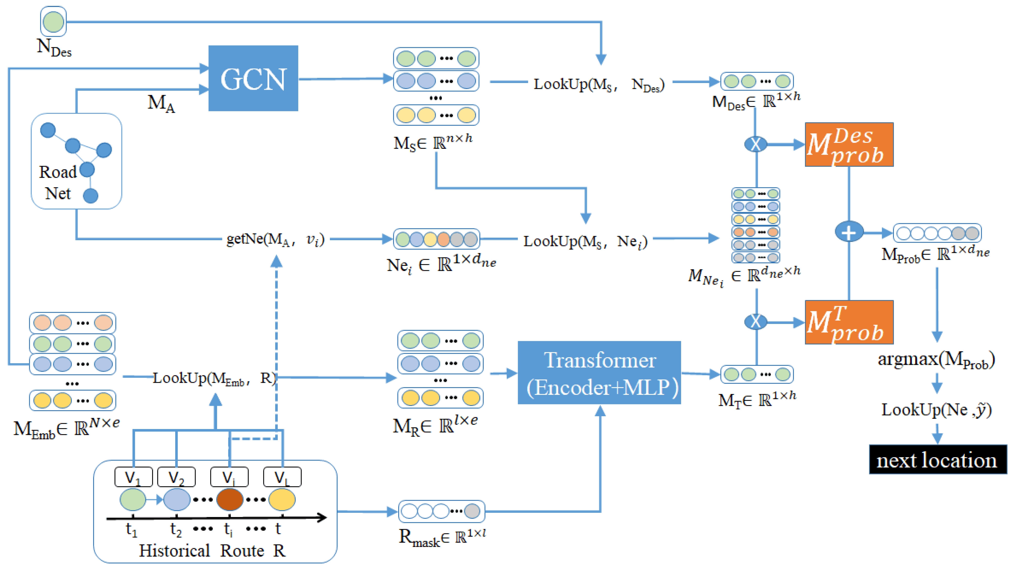
4. Methodology

In this paper, a model named Route Planning with Transformer (RoPT) is proposed to improve the accuracy of route planning in road networks. Existing approaches typically concatenate features of destination node with those of traversed node to predict the next node. However, due to the fact that the destination is more important than other nodes in route planning, in this paper, two prediction tasks are executed on destination and the current route composed of nodes that have been passed. The final results are computed on these two intermediate predictions results.

Firstly, with GCN, representations corresponding to spatial correlations of nodes are obtained, according to their adjacency matrix. Secondly, with Transformer, the representations of current route are captured based on concatenations of above node representations. Finally, based on the similarity between spatial representations of current route and the destination, and the similarity between temporal representations and spatial representations of current route, the next node of the route is recommended. As illustrated in Figure 1, RoPT is composed of three parts. The first part is the spatial feature aggregation module, which captures spatial representations of nodes on a road network with GCN, whose input are an adjacent matrix of a road network (M_A) and a learnable representation matrix of nodes (M_Emb). The second part is the sequence feature aggregation module based on Transformer, which captures temporal representations of nodes on long-term dependencies and sequential correlations in current route. The last part is next node prediction module, which calculates transition probabilities of nodes who are neighbors of current node in the route, according to representations of the destination and those neighboring nodes captured from results of the first part (GCN). In the end, the recommended neighboring node is the one with highest probability.

4.1. Spatial Feature Aggregation Module

Given that the road network is fundamentally a graph, within the RoPT framework, GCN is employed to capture the spatial representations of nodes by aggregating the features of both their direct and indirect neighbors. Specifically, the influence of direct neighbors is derived from the adjacency matrix of nodes. And the influence of indirect neighbors is obtained by iterative multiplication of the adjacency matrix. By stacking multiple layers of GCN, indirect influence from distant nodes is aggregated to enrich the latent spatial representations of current node. The specific calculation process is shown in Formula (3).

$$M_S^{\left(i\right)}=\left\{\begin{array}{c}\left({\tilde{D}}^{-{\displaystyle \frac{1}{2}}}\tilde{A}{\tilde{D}}^{-{\displaystyle \frac{1}{2}}}{M}_S^{\left(i-1\right)}{W}^{\left(i-1\right)}\right) if i=n\\ BN\left(\sigma \left({\tilde{D}}^{-{\displaystyle \frac{1}{2}}}\tilde{A}{\tilde{D}}^{-{\displaystyle \frac{1}{2}}}{M}_S^{\left(i-1\right)}{W}^{\left(i-1\right)}\right)\right) else\end{array}\right.$$

(3)

$$\tilde{D}=M_D+I,\tilde{A}=M_A+I,M_S^{\left(0\right)}=M_{Emb}$$

(4)

where $M_S^{\left(i\right)}\in {\mathbb{R}}^{n\times h}$ means the output of layer $i$ in this module, $M_{Emb}\in {\mathbb{R}}^{n\times e}$ is the node-embedding matrix to be learned, $I$ represents the identity matrix, $A$ represents the node adjacency matrix $M_A\in {\mathbb{R}}^{n\times n}$, $D\in {\mathbb{R}}^{n\times n}$ donates the degree matrix obtained from the adjacency matrix, $W^{\left(i\right)}\in {\mathbb{R}}^{n\times n}$ donates the weight matrix of layer $i$, $W^{\left(0\right)}, W^{\left(1\right)},{\dots , W}^{\left(l\right)}$ are learned with this model, and σ is an activation function. In addition, BN indicates a Batch Normalization function, to improve the stability of model training. Since there are other operations after GCN, BN and σ are not used in the last layer of this module. The final output of this module can be viewed as the spatial potential representations of all nodes $M_S\in {\mathbb{R}}^{n\times h}$.

4.2. Sequence Feature Aggregation Module

The purpose of this module is to capture temporal latent representations $M_T\in {\mathbb{R}}^{l\times h}$ of current route $R$ with Transformer. Since the length of original routes $R$ are different, the route $R$ with length less than $l$ should be padded to $l$, called $R^{*}$, as shown in Formula (5). Firstly, according to randomly initialized matrix of node features $M_{Emb}$, the $Lookup$ function is called to search the spatial potential representations of current route $R$, named $M_R\in {\mathbb{R}}^{l\times e}$, which is shown in Formula (6). With the $Lookup$ function, the corresponding row of $M_{Emb}$ is extracted according to the node ID, to obtain the representation matrix $M_R$ of $R$.

$$R[i]=\left\{\begin{array}{c}{R}^{*}\left[i\right]; if i \le \left|R^{*}\right|\\ \mathrm{pad}; if i>\left|R^{*}\right|\end{array}\right.$$

(5)

$$M_R=Lookup(M_{Emb},R)$$

(6)

Then, a mask vector of the route $R_{mask}$ is introduced to manually avoid obtaining representations of nodes in the padded positions, as shown in Formula (7). Here, $R_{mask}\in {\mathbb{R}}^l$ denotes the mask vector of $R$, the values of the padded positions are set as -inf to facilitate normalization of the attention mechanism, and those of rest positions are set as 0. Then, in Formula (8), $R_{mask}$ is converted into a mask matrix $M_{mask}$ by concatenating the route mask vector $R_{mask}$ for $l$ times, where rbind represents line-based concatenation. Next, $M_{mask}$ and $M_R$ are fed into the Transformer to obtain latent state $M_T$ of the route, as shown in Formula (9).

$$R_{mask}\left[j\right]=\left\{\begin{array}{c}0; if j \le \left|R^{\mathrm{*}}\right|\\ -inf; if j>\left|R^{\mathrm{*}}\right|\end{array}\right.$$

(7)

$$M_{mask}=rbind(\underset{l}{\underbrace{R_{mask}^T,R_{mask}^T,\dots , R_{mask}^T}}$$

(8)

$$M_T=Transformer(M_R,M_{mask})$$

(9)

$$Transformer\left(·\right)=MLP\left(LayerNorm\left(A\_N+FFN\right)\right)$$

(10)

$$A\_N=LayerNorm(M_R+MultiHead\left(GenIn\left(M_R\right),M_{mask}\right))$$

(11)

$$FFN=Relu\left(A\_N·W_1+b_1\right)W_2+b_2$$

(12)

In Formula (11), residual connection and Layer Normalization are used, also represented as A_N layer, where $LayerNorm(·)$ means the layer normalization operation. In Formula (12), the Feed-Forward layer is represented, where $W_1$ and $W_2$ are learnable weight matrices of the two linear layers, and $b_1$ and $b_2$ are biased. Next, the results are passed through an A_N layer again to obtain final outputs of the Encoder. As shown in Formula (10), an MLP is used as a Decoder, to transform the outputs of Encoder into latent representations of current route $M_T$, which is also the final output of Transformer.

The following is the specific calculation process of the Transformer. Firstly, the feature matrix of current route is calculated according to Formulae (13) and (14). Here, a linear layer is used to calculate the embedding of $M_R$, and position encoding of each step is added to obtain sequential features. Finally, temporal–spatial embedding matrix of route features is obtained as ${input}_E\in {\mathbb{R}}^{l\times h}$, where $M_{PE}$ donates the position matrix of the route, $pos\in [0,\mathrm{l}-1]$ donates the sequential step, and $i\in [0,\mathrm{h}-1]$ is the dimension index.

$${input}_E=GenIn\left(M_R\right)=\mathrm{L}\mathrm{i}\mathrm{n}\mathrm{e}\mathrm{a}\mathrm{r}\left(M_R\right)+M_{PE}$$

(13)

$$M_{PE}\left[pos,i\right]=\left\{\begin{array}{c}\mathit{sin}\left({\displaystyle \frac{pos}{{\mathrm{10,000}}^{\frac{i}{h}}}}\right);if i\%2=0\\ \mathit{cos}\left({\displaystyle \frac{pos}{{\mathrm{10,000}}^{\frac{i-1}{h}}}}\right);if i\%2=1\end{array}\right.$$

(14)

Then, calculations of multi-head attention are performed, where matrices of Query (Q), Key (K), and Value (V) are obtained from the input sequence with different linear transformation layers, and each head has its own independent matrices of Q, K, and V. In Formulae (15)–(17), the calculation process of each head and the integration of multi-head attention are shown, where $W_i^q\in {\mathbb{R}}^{h\times dk}$, $W_i^k\in {\mathbb{R}}^{h\times dk}$, $W_i^v\in {\mathbb{R}}^{h\times dv}$, and $W^O\in {\mathbb{R}}^{dv·he\times h}$, and $d_k=d_v=h/he$ donates the number of heads. It should be noted that, in Formula (16), the influence of padded nodes is removed when calculating self-attention. Here, using the theorem softmax(-inf) = 0, mask matrix $M_{mask}\in {\mathbb{R}}^{l\times l}$ is introduced to mask padded nodes.

$$MultiHead({input}_E,M_{mask})=Concat({head}_1,\dots ,{head}_{he})W^O$$

(15)

$${head}_i=softmax\left({\displaystyle \frac{Q{K}^T}{\sqrt{h}}}+M_{mask}\right)V$$

(16)

$$Q={input}_E{W}_i^q,K={input}_E{W}_i^k,V={input}_E{W}_i^v$$

(17)

4.3. Next Node Prediction Module

This module predicts the next node from latent representations of the destination node $N_{Des}$ and latent representations of the current route $M_S$. As shown in Formula (18), latent representations of the destination $M_{\mathrm{D}es}\in {\mathbb{R}}^{l\times \mathrm{h}}$ are looked up from the node representations output with GCN.

$$M_{Des}=LookUp(M_S,N_{Des})$$

(18)

Then, latent representations of neighboring nodes of current node $M_{\mathrm{N}\mathrm{e}\mathrm{i}}\in {\mathbb{R}}^{dne\times \mathrm{h}}$ are also obtained with the above methods. Here, the matrix of transition probability is computed with similarity calculation:

$${Ne}_i=getNe(M_A,v_i)$$

(19)

$$M_{{Ne}_i}=LookUp(M_V,{Ne}_i)$$

(20)

With Formula (19), latent presentations of neighboring nodes $N_{\mathrm{e}\mathrm{i}}\in {\mathbb{R}}^{l\times \mathrm{d}\mathrm{n}\mathrm{e}}$ of current node are found, where $M_A$ represents the network adjacency matrix, $v_i$ represents the current node, getNe is a function to search neighboring nodes of $v_i$, and IDs of neighboring nodes are concatenated into a vector $N_{\mathrm{e}\mathrm{i}}\in {\mathbb{R}}^{l\times \mathrm{d}\mathrm{n}\mathrm{e}}$. When the number of neighbors is less than the hyper-parameter $d_{ne}$, it should be padded to $d_{ne}$. Then, the representations of the neighbors of current node $M_{\mathrm{N}\mathrm{e}\mathrm{i}}$ are obtained with Formula (20).

Next, transition probability based on current route is calculated $M_{Prob}^T\in {\mathbb{R}}^{l\times \mathrm{d}\mathrm{n}\mathrm{e}}$.

$$M_{prob}^T={\displaystyle \frac{exp(M_{{Ne}_i}·M_T)}{\sum _{i}exp(M_{{Ne}_i}·M_T)}}$$

(21)

Similarly, transition probability based on destination $M_{Prob}^{Des}\in {\mathbb{R}}^{l\times \mathrm{d}\mathrm{n}\mathrm{e}}$ can also be calculated.

$$M_{prob}^{Des}={\displaystyle \frac{exp(M_{{Ne}_i}·M_{Des})}{\sum _{i}exp(M_{{Ne}_i}·M_{Des})}}$$

(22)

Then, the calculation of complete transition probability ${\mathrm{M}}_{\mathrm{prob}}\in {\mathbb{R}}^{\mathrm{l}\times \mathrm{d}\mathrm{n}\mathrm{e}}$ is shown in Formula (23), where $\lambda$ is a hyper-parameter to balance importance of the two transition probabilities listed above. The index of the position with the highest probability is obtained by the argmax function.

$$M_{\mathrm{prob}}=(1-\lambda )M_{\mathit{prob}}^{\mathit{Des}}+\mathsf{\lambda }{M}_{\mathit{prob}}^T$$

(23)

Finally, a Cross-Entropy Loss function is used to train the whole model RoPT, which is shown in Formula (24).

$$Loss=-{\displaystyle \frac{1}{n}}{\sum }_i{\sum }_{c=1}^{dne}q\left(y_{ic}\right)log\left(p_{ic}\right)$$

(24)

Here, $y_{ic}$ denotes the index of node in the real route. And q denotes a signum function, whose output is 1 when, in sample i, the index is equal to the real index; otherwise, it is 0. The transition probability of each node in sample $i$ is denoted as $p_{ic}$.

5. Experiments

5.1. Datasets

The experiments are conducted on real-world trajectory datasets from two cities, Porto [2] and Chengdu, with their statistical characteristics summarized in

Table 2. Statistics of datasets.

	Chengdu	Porto
number of nodes	3041	5330
number of edges	4354	11,491
number of trajectories	5,887,769	1,258,165
sparsity	0.698	0.463
mean trajectory length	23.09	40.21

. The former is denoted as the Porto Dataset, which is an open dataset of 18 GB, recording taxi trajectories between 7 January to June 2013. The latter is denoted as the Chengdu dataset with a size of 60 GB, which is composed of taxi trajectories from 1 November to 30 November 2016. The Chengdu dataset only contains GPS coordinates without road segment information; the road network and the corresponding adjacent graph of Chengdu is constructed from OpenStreet-Map [30] for matching GPS locations to road sections [31]. Here, the sparsity of the dataset is calculated as the ratio of the number of nodes to the number of edges, which means a node equally appears on how many edges.

Preprocessing of datasets: First, discontinuous routes are eliminated. If the time between two consecutive points in a route is bigger than 30 s, then the route is divided into two parts. Secondly, Leuven MapMatching based on a Hidden Markov Model (HMM) is used to map GPS trajectory points to the actual road network obtained from OpenStreetMap.

5.2. Experiment Settings

Environment. The machine used in the experiments is equipped with a 2.50 GHz Intel(R) Xeon(R) Platinum 8255C CPU, and an NVIDIA GTX 3080 GPU with 24 GB VRAM. Our model RoPT is developed on Python 3.8 and PyTorch 1.13.

Hyper-parameter. The datasets are partitioned in an 8:1:1 ratio into training, validation, and test sets. The average number of neighbors of each node in the Chengdu dataset is 4.34, while that of Porto is 2.39. The dimensions of the initial feature matrix of a road network $M_A$ is set as 128. The number of layers of the GCN is set as 4. The output dimensions of each layer are 64, 128, 256, and 256. The number of heads in the encoder of the Transformer is set as 8, whose number of layers is set as 3, and the dimension is set as 256. The number of layers of the MLP corresponding to the decoder is also set as 3, and the dimension is 256. These hyper-parameters conform to those used in the baselines which follow the best settings listed in the references. The analysis of choosing 4 as the number of layers of the GCN is detailed as described in Section 5.6.

Evaluation Metric. For the route-planning task, we adopt the standard performance metrics [1,2,3,6,32]:

(1) Acc, (2) Recall, (3) F1, and (4) Acc@K, (k = 1).

The first three metrics are used to evaluate the performance of a recommended full route, and the fourth Acc@K is used to evaluate the performance of a recommended next node. Their calculation formulae are shown in Formulae (25)–(27):

$$Acc={\displaystyle \frac{|R\cap R^{*}|}{\left|R^{*}\right|}} Recall={\displaystyle \frac{|R\cap R^{*}|}{\left|R\right|}}$$

(25)

$$F1={\displaystyle \frac{2\ast Acc\ast Recall}{Acc+Recall}}$$

(26)

$$Acc@k={\displaystyle \frac{1}{\left|R^{*}\right|}}{\sum }_{i=1}^{\left|R^{*}\right|}1\left({rank}_i<k\right)$$

(27)

Here, $R$ is a route recommended with model PoPT, $R^{*}$ is the corresponding real route, the intersection of these two routes represents the set of common nodes, the symbol similar to the absolute value represents the cardinality of the intersection, and ${rank}_i$ is the position of the i-th recommended node ranked with the transfer probability in the current reachable node set.

5.3. Baselines

To better evaluate the performance of RoPT, the following baselines are chosen for comparison:

Dijkstra: A traditional method for finding the shortest path from the source node to the destination node, where the weight of an edge corresponds to the time consumption of the edge in the road network.

Heuristic-A* [32]: In this method, when computing the edge cost, traffic and weather conditions are considered in the penalty term of the edge cost in A*. Due to the fact that weather condition is not considered in other baselines, only traffic congestion is considered in our simulated method.

CSSRNN [1]: In this method, route planning is carried out with the spatial correlations of nodes in the road network extracted based on the node reachable matrix, and sequence correlations in the trajectory extracted based on the RNN.

GETNext [3]: In this method, a global flow graph based on trajectories is constructed. Firstly, the potential representations of nodes are learned with the GCN, then the embedded information, such as the movement mode, user, node, and time, are combined and fed into the Transformer to predict the next node to be visited. Due to the fact that this method is only designed for predicting the next POI, in order to improve its performance in route planning, destination information is added into the Transformer in the following experiments. The method of adding the destination is similar to RoPT: destination embedding learned from the GCN is added to the end of the current route.

GetNext-N is a variant of GetNext that considers only neighboring nodes when calculating the transition probability.

NEUROMLR [2]: In this method, a GCN and Lipschitz embedding are used in order to learn the potential representations of nodes. To reduce the dimension of the temporal features of a node, which is formed with concatenating the potential representation of the node in all time slices, Principal Component Analysis (PCA) is introduced. Finally, the transition probability can be predicted on representations of the node to be transferred, the current node, and the destination node.

Graphormer [6]: This method incorporates the structure of a graph into the Transformer via three encoding techniques. Centrality encoding adds learnable embeddings based on the node degree to the initial features. Spatial encoding uses the shortest path distance (SPD) to model the spatial relationships between nodes. Edge encoding adjusts attention weights by averaging the dot products of edge features and learnable embeddings along the shortest paths. These encodings allow Graphormer to capture both local and global graph dependencies, achieving strong performance across graph representation tasks.

5.4. Performance Comparisons

In

Table 3. Overall performance comparisons (the values in bold represent the best, the values with underline represent the second best, and the line of “improvement” compares RoPT with the second best).

	Porto				Chengdu
	Acc	Recall	F1	ACC@1	Acc	Recall	F1	ACC@1
Dijkstra	63.42%	50.20%	56.04%	63.42%	55.73%	41.91%	47.84%	55.73%
A*	64.82%	54.37%	59.14%	64.82%	49.04%	44.30%	46.55%	49.04%
Heuristic-A*	66.55%	55.89%	60.76%	66.55%	52.74%	46.83%	49.61%	52.74%
CSSRNN	65.23%	68.84%	66.98%	92.70%	56.12%	54.33%	55.21%	80.56%
Graphormer	15.67%	40.12%	22.54%	75.40%	23.46%	42.56%	30.25%	68.43%
GetNext	7.73%	27.53%	12.07%	66.37%	11.07%	33.22%	16.60%	59.05%
GetNext-N	66.02%	68.92%	67.43%	92.83%	56.08%	55.65%	55.86%	80.81%
Neuro	74.13%	71.24%	72.65%	94.83%	61.85%	60.77%	61.30%	84.41%
RoPT (Ours)	75.62%	71.30%	73.40%	95.36%	62.85%	61.42%	62.00%	85.61%
Improvement	+1.49%	+0.06%	+0.75%	+0.53%	+1.00%	+0.65%	+0.7%	+1.20%

, the performances of our model RoPT on two datasets are shown, compared to other baselines. Overall, RoPT achieves optimal performance on several metrics. And Neuro performed second best. This can be attributed to Porto’s lower average node degree (2.39), which simplifies target identification within the top two recommendations. Similarly, all the metrics in the Chengdu dataset are lower than those in the Porto dataset because the number of neighbors per node in the Chengdu dataset is 4.34, much bigger than that in Porto, which increases the difficulty of recommendation.

The reason why RoPT performs better stems from the fact that it captures the temporal correlations of nodes in trajectories with the Transformer, and captures the spatial correlations of nodes in the road network with the GCN. In contrast, in Neuro, only the average speed of edges in the different periods is focused on, and the order of nodes in trajectories is not fully considered. Although CSSRNN incorporates node sequence information and road network constraints, it fails to conduct an in-depth analysis of spatial correlations among road network nodes. Even in Graphormer, where the Transformer is used, the spatial correlations of nodes are modeled statically with the shortest path distance, which degrades its performance. GetNext similarly combines the GCN and Transformer; yet, its full-node prediction strategy introduces unnecessary complexity for node recommendation tasks. To address this, in GetNext-N, a variant of GetNext, only neighbor nodes are considered when recommending the next node. It can be found that all metrics of GetNext-N are better than those of GetNext, which indicates the necessity of limiting the ranges of candidates.

5.5. Ablation Studies

To verify the effectiveness of the GCN, Transformer, and destination information, ablation experiments are conducted on the Porto and Chengdu datasets, with results shown in

Table 4. Ablation results (the values in bold represent the best).

	Porto		Chengdu
	Acc	Recall	Acc	Recall
RoPT (Ours)	75.81%	71.47%	62.91%	61.82%
w/o MDes	66.75%	60.38%	58.59%	55.65%
w/o Transformer	72.46%	67.91%	61.88%	60.17%
w/o GCN	70.80%	64.32%	60.97%	59.96%

. The method marked as w/o $M_{Des}$ represents the variant of removing destination, w/o Transformer represents the variant of replacing the Transformer with an RNN, and w/o GCN represents the variant of replacing the GCN with a linear layer. The results reveal that destination information exerts the most significant impact. Destination removal leads to a performance degradation of 9.06% (Acc) and 11.09% (Recall) on Porto, and 4.32%/6.17% on Chengdu, correspondingly. The biggest reason may stem from the fact that, when taking a taxi, passengers like to take the expressway to reach their destination as soon as possible. As we know, the number of forks on the expressway are few, so the choice of route is simple, which increases the impact of the destination. After the removal of the GCN and Transformer, the metrics are also decreased, which prove the effectiveness of the combination of the GCN and Transformer. Notably, the GCN demonstrates greater influence, aligning with the well-established principle that spatial road network correlations are prioritized in route planning.

5.6. Hyper-Parameter Analysis

In this section, the influence of λ and the number of GCN layers are investigated. The change in λ will affect the importance ratio of the passed nodes and destination. While a deeper GCN can capture more complex graph correlations, they may compromise the generalization performance. Exploring the appropriate number of GCN layers is helpful in order to promote the RoPT model. The results are shown in Figure 2a and Figure 2b, respectively. Figure 2a demonstrates peak Recall at λ = 0.5, revealing an equivalent importance between the historical trajectory nodes and destinations. This suggests that temporal feature extraction and spatial modeling hold equal importance. From Figure 2b, the performance of Recall tends to be stable after the number of GCN layers reaches 4, indicating that the long-distance node has little influence on the next node. For this purpose, a 4-layer GCN is used to extract spatial features.

5.7. Qualitative Study

To better illustrate the correspondence between the extracted node latent representations and the real road network, t-SNE is employed to perform dimensionality reduction on node features extracted with RoPT and Neuro on the Chengdu dataset. We fix the t-SNE random seed at 20150101 while retaining scikit-learn’s TSNE default parameters for all other hyper-parameters. The detailed results are shown in Figure 3 where each point corresponds to a node in the road network. The position of the center point corresponds to the mean longitude and latitude of the nodes in the trajectories. The city was then divided into four parts based on the horizontal and vertical axes. The nodes in the northeast, southeast, northwest, and southwest parts are marked in pink, blue, yellow, and green.

As shown in Figure 3a, the points in these four colors are relatively clustered, where green points are mainly located on the margins of the upper part, yellow points are mostly in the middle, pink points are concentrated in the southwest, and blue points, though more dispersed, can be observed to cluster roughly into two groups in the northeastern and southwestern parts. In contrast, in Figure 3b, the points of different colors are more scattered. The pink points clustered in the north are interspersed with many yellow points, and the blue points clustered in the west are also mixed with a large number of green, yellow, and some red points. Notably, the eastern yellow clusters and southern green clusters both demonstrate pronounced heterogeneity through admixture with other colored points. To further demonstrate the effectiveness of the feature extraction, several consecutive segments of a road are chosen and highlighted in Figure 3a,b. Here, red triangles correspond to several continuous segments on the northern part of the Chengdu Ring Road, which are also circled in the figure. As in Figure 3a, with the latent representations learned with RoPT, these segments are clustered closely on the right side of the figure. Conversely, Neuro’s representations result in the significant dispersion of these segments. Especially, the segment located in the leftmost circle in Figure 3b is far away from the other segments. This phenomenon demonstrates that RoPT is more effective in capturing the correlations between nodes in the road network.

5.8. Reasoning Efficiency

It is well-established that deep-learning models typically exhibit a longer inference latency compared to classical algorithms like A*. Thus, an experiment is carried out on the Chengdu dataset, to show the limitations of RoPT in reasoning efficiency. From

Table 5. Reasoning efficiency (average inference time and standard deviation for each route planning in Chengdu dataset—the values in bold represent the best and the values with underline represent the second best).

	Average Inference Time (ms)	Standard Deviation (ms)
A*	0.278	0.174
Heuristic A*	11.692	6.964
CSSRNN	242.951	22.409
Neuro	298.215	27.682
GetNext	308.423	29.455
RoPT (ours)	297.631	23.630

, it can be seen that the average inference time of A* and Heuristic A* are much shorter than other deep-learning-based methods. However, considering deep-learning-based methods, such as CSSRNN, Neuro, GetNext and RoPT, the average inference time of RoPT is only longer than CSSRNN, which comes from the well-known fact that the inference time of the Transformer is longer than the RNN. And the standard deviation of RoPT is significantly reduced, indicating that it is better for handling complex spatial–temporal correlations.

It is also known that A* is not suitable for traffic environments changing dynamically. Therefore, in the future, a trade-off could be made so that, when traffic environments remain stable, A* and its variant are used; otherwise, RoPT and other deep-learning-based methods are used.

6. Conclusions and Future Work

In this paper, a route-planning model, named RoPT, is proposed for use in an urban transportation system. The use of RoPT can capture drivers’ experience in order to recommend routes that are less time-consuming to users with navigation apps, helping administrative traffic management discover abnormal road sections, and so forth. In RoPT, the GCN and Transformer are combined in order to handle complex spatio-temporal correlations in traffic, where the spatial representations of nodes in the road network are captured with stacking multi-layer GCNs and the temporal representations of nodes in trajectories are captured with the Transformer. Furthermore, considering that the destination has a great influence on route planning, in RoPT, features of the destination, captured from the graph corresponding to the road network, are combined with latent representations of the current trajectory to predict the next road section more accurately. The experimental results from the Porto and Chengdu datasets demonstrate that RoPT achieves consistent improvements over baselines, with relative gains of 1.49% (Accuracy), 1.00% (Recall), and comparable F1/Acc@1 scores. And latent features learned with RoPT are more interpretable.

Our inference time experiments demonstrate that deep-learning-based methods exhibit a significantly bigger computational cost compared to A* and its variants. In the future, we will explore methods of route planning which combine the advantages of these two types, according to the dynamics of traffic environments.