Article

Evaluation of Rural Visual Landscape Quality Based on Multi-Source Affective Computing

1
School of Art and Design, Dalian Polytechnic University, Dalian 116034, China
2
School of Design, Dalian Minzu University, Dalian 116600, China
*
Author to whom correspondence should be addressed.
These authors contributed equally to this work.
Appl. Sci. 2025, 15(9), 4905; https://doi.org/10.3390/app15094905
Submission received: 25 March 2025 / Revised: 19 April 2025 / Accepted: 24 April 2025 / Published: 28 April 2025

Abstract

:
Assessing the visual quality of rural landscapes is pivotal for quantifying ecological services and preserving cultural heritage; however, conventional ecological indicators neglect emotional and cognitive dimensions. To address this gap, the present study proposes a novel visual quality assessment method for rural landscapes that integrates multimodal sentiment classification models to strengthen sustainability metrics. Four landscape types were selected from three representative villages in Dalian City, China, and the physiological signals (EEG, EOG) and subjective evaluations (Beauty Assessment and SAM Scales) of students and teachers were recorded. Binary, ternary, and five-category emotion classification models were then developed. Results indicate that the binary and ternary models achieve superior accuracy in emotional valence and arousal, whereas the five-category model performs least effectively. Furthermore, an ensemble learning approach outperforms individual classifiers in both binary and ternary tasks, yielding a 16.54% increase in mean accuracy. Integrating subjective and objective data further enhances ternary classification accuracy by 7.7% compared to existing studies, confirming the value of multi-source features. These findings demonstrate that a multi-source sentiment computing framework can serve as a robust quantitative tool for evaluating emotional quality in rural landscapes and promoting their sustainable development.

1. Introduction

Amid the dual forces of accelerating global urbanization and the concurrent antiurbanization trend, the rural landscape is undergoing an unprecedented transformation in value. In the postindustrial era, reflections on the “over-technicalization” of urban spaces have led to the social practice of “re-localization”, prompting a reassessment of the strategic importance of rural areas as the foundation of ecological resilience and cultural heritage [1]. While the implementation of China’s rural revitalization strategy has progressively elevated rural environments by “underdeveloped areas” to central fields for “ecological-cultural-economic collaborative revitalization”, the assessment of rural landscape sustainability remains mired in significant quantitative challenges. Although traditional ecological indicators (such as soil and water conservation rates and biodiversity indices) can depict the physical attributes of natural resources, they fail to capture the underlying forces of emotional carrying capacity in human settlements and the visual cognitive experience influencing community identity and ecological behavior [2]. This issue arises from the methodological limitations of a one-dimensional approach, where the “hard-data” of ecosystems and the “soft-value” of human emotions have long existed in a disciplinary divide [3]. As an emerging interdisciplinary innovation, emotional computing technology, through its (1) theoretical evolution, (2) technological breakthroughs, and (3) paradigm shifts, constructs a quantitative sustainability framework that integrates multi-source emotional computing with rural visual landscapes, unveiling the synergistic potential between the two.

1.1. Affective Computing

Emotion, as a complex psychophysiological phenomenon, plays a pivotal role in daily life [4]. A positive emotional state is essential for maintaining both physical and mental wellbeing, while prolonged negative emotions can profoundly affect an individual’s health [5]. Consequently, the study of emotional states has expanded across multiple disciplines, including neuroscience, psychology, medicine, biology, computer science, engineering, and the humanities, gradually fostering an interdisciplinary development trend [6,7,8,9,10]. For instance, in neuroscience, emotional research focuses on the neural mechanisms underpinning emotions; in psychology, it explores how emotions influence human behavior, resulting in physical and psychological changes; and in computer science, it encompasses the study and analysis of emotional responses, commonly referred to as affective computing, which has garnered increasing attention in recent years. Affective computing serves as an umbrella term for human emotion recognition and analysis [6]. As a cornerstone in the advancement of human-centered artificial intelligence and human–computer interaction [11], emotional computing has enabled computers to recognize, express, and respond to both their own emotions and those of humans, a concept introduced by Professor Picard in 1997 [12,13]. In practical applications, emotional computing has been employed across diverse fields such as healthcare, education, business services, intelligent driving, social media, and the integration of science and art [14,15,16,17,18,19], where it is used to identify users’ emotional states and provide appropriate feedback and adjustments.

1.2. Multi-Source Affective Computing

Multi-source emotion computing refers to the application of experiments utilizing multi-source data in emotion computing, aiming to transition from single-mode to multi-source data [20], transcending modal boundaries to achieve a higher emotion recognition rate [21,22]. Its research framework encompasses two core themes and five key aspects (as depicted in Figure 1). The two themes are emotion recognition and emotion analysis, while the five aspects include the foundational theory of emotion, signal collection, algorithm modeling, modal fusion, and output presentation, which may overlap and interrelate. In the domain of emotion recognition, the focus is on detecting human emotional states (i.e., discrete or dimensional emotions) through visual, auditory/speech, and physiological modalities. Sentiment analysis, on the other hand, primarily centers on evaluating and extracting preferences for objects or events [23], with results typically categorized as positive, negative, or neutral [24,25]. Among the five aspects, the first is the foundational theory of emotions. Psychologists have proposed two primary models—the discrete emotion model and the dimensional emotion model—to simulate human emotions from basic to complex states [26,27]. The second aspect concerns the collection of emotional signals. Recent advancements have seen the use of various physiological signals, such as electroencephalogram (EEG), electromyogram, electrocardiogram, and eye movement, alongside non-physiological signals, including text, speech, facial expressions, and body movements, all of which contribute to emotion recognition, supported by corresponding datasets [28,29,30]. Notably, EEG signals have been shown to outperform other physiological signals in emotion recognition tasks [31,32], while eye movement signals complement EEG data in multimodal emotion recognition scenarios [33,34], enhancing the accuracy of multimodal emotion classification systems. The third aspect, algorithm modeling of emotion, involves leveraging machine learning, ensemble learning, and deep learning techniques to model and identify emotional signals. Common classifiers for environmental emotion recognition include Logistic Regression, Support Vector Machines (SVMs), Decision Trees, ensemble models, and neural networks [35,36,37]. The fourth aspect, modal fusion, integrates emotional features and fusion algorithms derived from multimodal recognition to enhance emotion classification accuracy [38]. The fifth aspect is the output presentation of emotion, which enables machines to express emotions through facial expressions, vocal intonation, body movements, and visualization platforms, following the learning of emotional signals [39], thereby advancing human–computer interaction. Therefore, sentiment analysis utilizing multi-source data plays a pivotal role [40] and has been increasingly validated in sentiment classification and event detection applications [30,41].

1.3. Rural Visual Landscape Quality Assessment

As a spatial–cultural composite that embodies the evolving human–land relationship, the assessment of rural landscape visual quality plays a pivotal role in quantifying ecological service functions and preserving cultural memory [42,43]. In contrast to the homogenizing trends observed in urban landscapes, the regional heterogeneity of rural visual landscapes, coupled with the interplay between natural and human elements, facilitates a paradigm shift in evaluation—from traditional aesthetic criteria to interdisciplinary collaborative analysis [44]. The theoretical foundation for visual landscape quality assessment can be traced to Laurie’s concept of “the comparative relationship between the perception and evaluation of two or more landscapes” [43]. In the rural context, this concept is further extended to encompass “the systematic decoding of the visual characteristics and emotional value of local spaces”. Methods for assessing the quality of rural visual landscapes can be categorized into two distinct approaches [45]. The first, “externalist” evaluation, treats space as an object of observation. Common methods, such as GIS [46] and surveys [47], are employed to analyze stimuli including remote sensing images, classified maps, photographs, and actual landscapes. The second approach is “egocentric” assessment, which typically begins with direct human experience and employs physiological sensors—such as eye trackers [48] and EEG [47]—along with evaluative tools such as the Scenic Beauty Estimation (SBE) method [49], Analytic Hierarchy Process (AHP) [50], and Semantic Differential (SD) method [51]. This approach combines intuitive perception and assessment of photos, simulations, and real landscapes, incorporating both objective and subjective evaluations (through questionnaires). In addition to these two evaluation methods, the interdisciplinary integration of neuroscience, psychology, computer science, and visual landscape research has led to the development of techniques for random visual landscape perception, evaluation, and emotion classification prediction. For example, Ningning Ding et al. [52] analyzed the preferences of villagers and university students using eye tracking and EEG to explore the appeal of plant organ structures. They found that plants with distinct features and vibrant colors were preferred in rural landscapes, while simpler structures were favored in campus settings. Feng Ye et al. [53] developed a predictive model based on the correlation between eye-tracking metrics and 19 different emotional responses to rural landscapes, highlighting the effectiveness of eye-tracking technology in capturing and predicting emotional reactions to various landscape types. Wang Yuting et al. [54] innovatively employed aerial video and EEG technologies to assess rural landscapes, selecting seven representative landscape types, extracting EEG features, and classifying them with four classifiers. They demonstrated that SVM and Random Forest (RF) classifiers exhibited high accuracy, achieving 98.24% and 96.72%, respectively, and identified distinct classification patterns across different features and bands, thereby advancing novel methodologies for quantifying human perception. Thus, in the assessment of rural visual landscape quality, perception refers to the behavioral patterns of visual or brain activity, while evaluation pertains to preferences and ratings of the landscape. Both processes are intrinsically linked to the emotional experience of the visual landscape.

1.4. Summary of Relevant Research

In summary, the primary challenges in rural visual landscape affective computing research are as follows: (1) Insufficient interdisciplinary integration in rural landscape affective computing. Although affective computing technology has been extensively applied in fields such as healthcare, education, and urban design, its comprehensive integration into rural landscape visual quality assessment remains underdeveloped. (2) Limited collaborative classification of multimodal data and subjective questionnaires. While the fusion of objective modes, such as eye tracking and EEG, has been explored in multi-source affective computing, few datasets have been developed that use subjective questionnaire data as independent variables. (3) Existing studies lack systematic verification of the adaptation rules for classifier performance. Most research defaults to using a single classifier (e.g., SVM or Random Forest) to process emotion classification tasks across various categories, overlooking the boundary effects of task complexity on model performance. This leads to challenges such as difficulties in adaptive multi-source feature fusion, weak scene generalization, and small sample overfitting. In response, this study selected twelve rural landscape images, representing four distinct types from Dalian, Liaoning, China, as stimuli. It collected emotional signals using a combination of subjective and objective methods (“eye movement + EEG + questionnaire score”) from participants, and applied machine learning and ensemble learning techniques to develop an emotion classification model and spatial emotion quality assessment process. This approach is applicable to a variety of rural visual landscape quality assessments, with the final evaluation results providing valuable insights for rural landscape design and decision-making in rural revitalization.
This paper is structured into five sections: Section 1 provides an overview of the prior research. Section 2 introduces the study area, data, and methodologies employed. The key findings are presented and analyzed in Section 3. Section 4 discusses the results, along with the study’s limitations. Finally, Section 5 presents the conclusions.

2. Materials and Methods
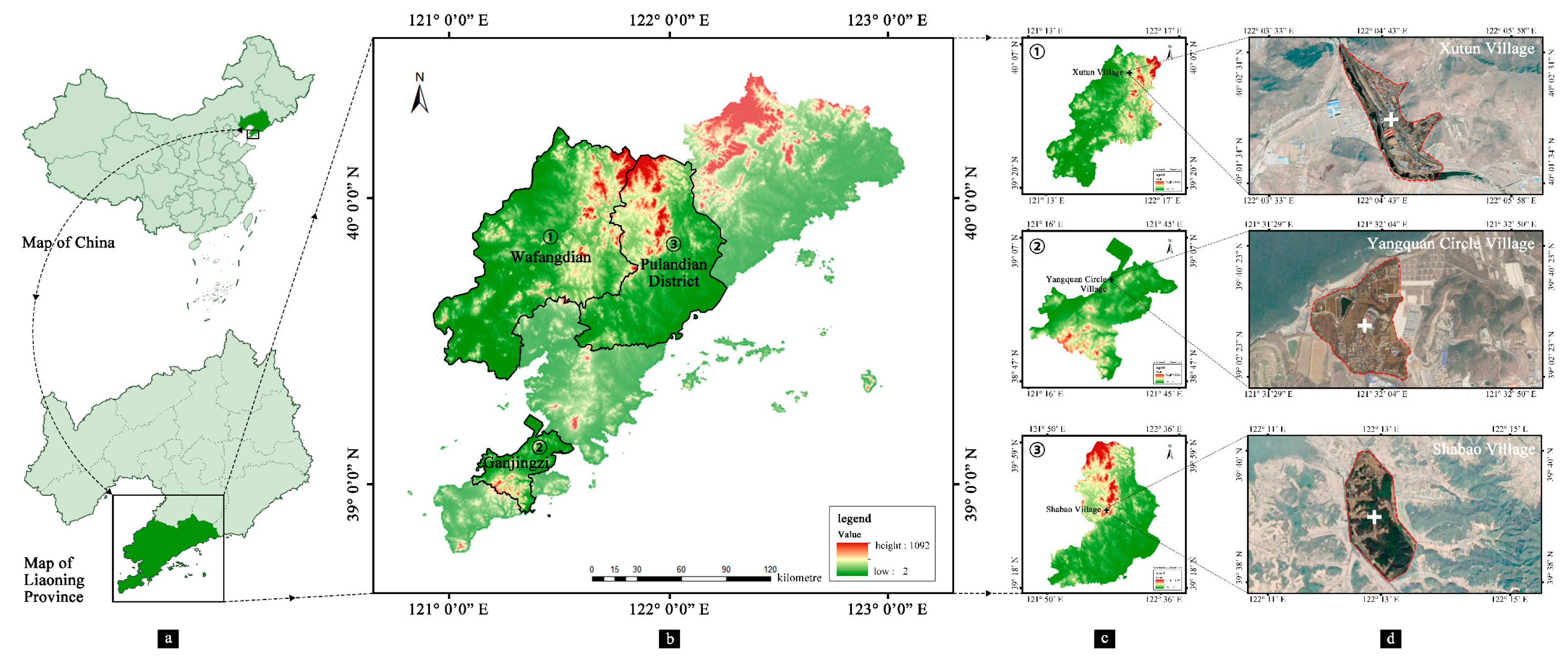
2.1. Research Area

Dalian, situated in the southern part of Liaoning Province (120.58° E to 123.31° E, 38.43° N to 40.10° N), as depicted in Figure 2a, is renowned as the “Pearl of the North” and is a popular tourist destination. In addition to its rich marine culture, Dalian’s villages exhibit a diverse range of forms and regional characteristics, making it an ideal setting for rural visual landscape quality assessments. Therefore, three representative villages within Dalian were selected for investigation in this study: (1) Xutun Village, a traditional settlement located in Xutun Town, Wafangdian City, known for its long history and distinctive architectural style, which primarily focuses on restoration and conservation; (2) Yangquan Circle Village, a coastal village situated in Gezhenbao Street, Ganjingzi District, where the village’s development is influenced by a “medium intervention” approach from architects and urban planners; and (3) Shabao Village, a rural settlement in Shabao Street, Pulandian District, which has undergone spontaneous, top-down construction and renovation by the villagers themselves (as shown in Figure 2c,d). Field investigations were conducted, and key landscape features of the villages were photographed to serve as a foundation for the multi-source emotion computing experiments.

2.2. Experimental Elements

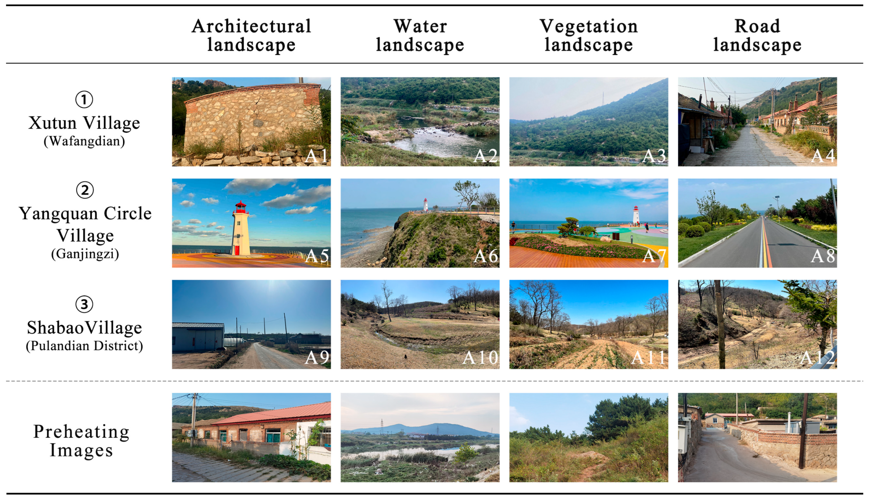
2.2.1. Element Presentation

Given the constraints of human and material resources for onsite landscape evaluation, landscape photographs were selected as substitutes for direct environmental investigations [55]. To ensure the subjects’ perceptions closely align with real-world experiences, virtual scenes, which could distort visual perception, were avoided [56,57,58]. Consequently, original images were utilized in this study, with all images sized at 1920 × 1080 pixels, rather than edited landscape photographs. A SONY A6000 SLR (SONY, Tokyo, Japan) camera was employed to capture landscape samples from a distance of 8 m and at a height of 1.6 m from the edge of the object space. The photos were taken from November 2023 to May 2024, resulting in a total of 360 images.
During the photo-selection process, five experts classified the images according to the following procedure: (1) Feature Annotation: Reviewed 360 photographs, extracted salient keywords for landscape elements (such as buildings, water bodies, vegetation, roads, etc.), and annotated each image’s core attributes. (2) Unrestricted Classification: Grouped images sharing similar annotated features. (3) Consolidation: Considering overlap or redundancy among the 360 photographs, provisionally sorted them into four categories—architecture, water, vegetation, and roads—with ten images per group. (4) Validation and Refinement: Experts scored and cross-referenced each category, reducing each group to five or six images. (5) Representativeness Assessment: Based on each village’s characteristics, retained the three most representative images per category. This process yielded a structured library of 12 landscape images from three villages to support subsequent experimental research. To mitigate potential bias from priming effects, four additional images were chosen as warm-up stimuli for the experiment (as shown in Figure 3).

2.2.2. Experimental Subjects

To facilitate the experiment, 35 students and 3 teachers (17 males, 21 females; average age: 25.63 years) participated. Of these, 23 were aged between 20 and 25 years, 11 between 25 and 30 years, 1 between 30 and 39 years, and 3 between 40 and 45 years. All participants were right-handed, with no history of mental illness or brain trauma, and had normal or corrected vision, except in the campus environment. None of the participants had previously visited the experimental site. Four participants were excluded from the final analysis due to signal artifacts, leaving data from 34 participants (17 males and 17 females) for analysis. All participants voluntarily consented to the study, having received full information regarding the research objectives, experimental procedures, and potential risks. They signed written informed consent prior to participation and were compensated upon completion, with the option to withdraw at any time without penalty.

2.2.3. Experimental Equipment and Questionnaire

The experimental setup comprised an Eyeso Glasses head-mounted eye tracker (Braincraft, Beijing, China) and a Waveguard™ 8-lead electrode cap (ANT Neuro, Berlin, Germany). The eye movement sampling rate was 380 fps, and the EEG was recorded via a 500 Hz micro-EEG amplifier. Supporting equipment included a 24-inch display (resolution 1920 × 1080), a laptop (running Windows 10), a dongle, and an adapter for convenient mobile portability. The laptop also served as the medium for displaying the landscape images (as shown in Figure 4). The experimental questionnaires were categorized into two sections: (1) The Beauty Assessment Scale and (2) The SAM Scale. (1) The Beauty Assessment Scale is a subjective tool for quantifying individuals’ visual experiences of landscapes. It integrates the SBE (Scenic Beauty Estimation) scale with the SD (Semantic Differential) method to create a streamlined evaluation framework, enabling participants to intuitively rate landscape aesthetics—higher scores correspond to greater perceived beauty. The SBE method quantifies the landscape’s aesthetic appeal based on evaluators’ personal standards [49], while the SD method employs a verbal scale to conduct psychological measurements of individuals’ intuitive responses [51], providing quantitative data for landscape assessment. Based on the works of Liu Binyi et al. [59] and Xie Hualin et al. [60], and considering the specific visual characteristics of rural landscapes in Dalian, eight semantic variables were chosen as evaluation criteria: naturalness (N), diversity (D), harmony (H), singularity (S), orderliness (O), vividness (V), culture (C), and agreeableness (A). (2) The SAM Scale (as shown in Figure 5) [61] is a versatile tool designed to track emotional responses to stimuli across various settings, enabling quick assessment of emotional reactions. During the experiment, participants’ emotional states were recorded through the SAM questionnaire, capturing both emotional valence (positive or negative) and arousal (high or low). Both questionnaires were rated using a 5-point Likert scale, with scores ranging from −2 (lowest) to +2 (highest) [62]. By synthesizing subjective impressions with objective measurements, the evaluation of landscape aesthetics can more fully elucidate visual allure and underpin a rigorous scientific basis for the sustainable design of rural landscapes.

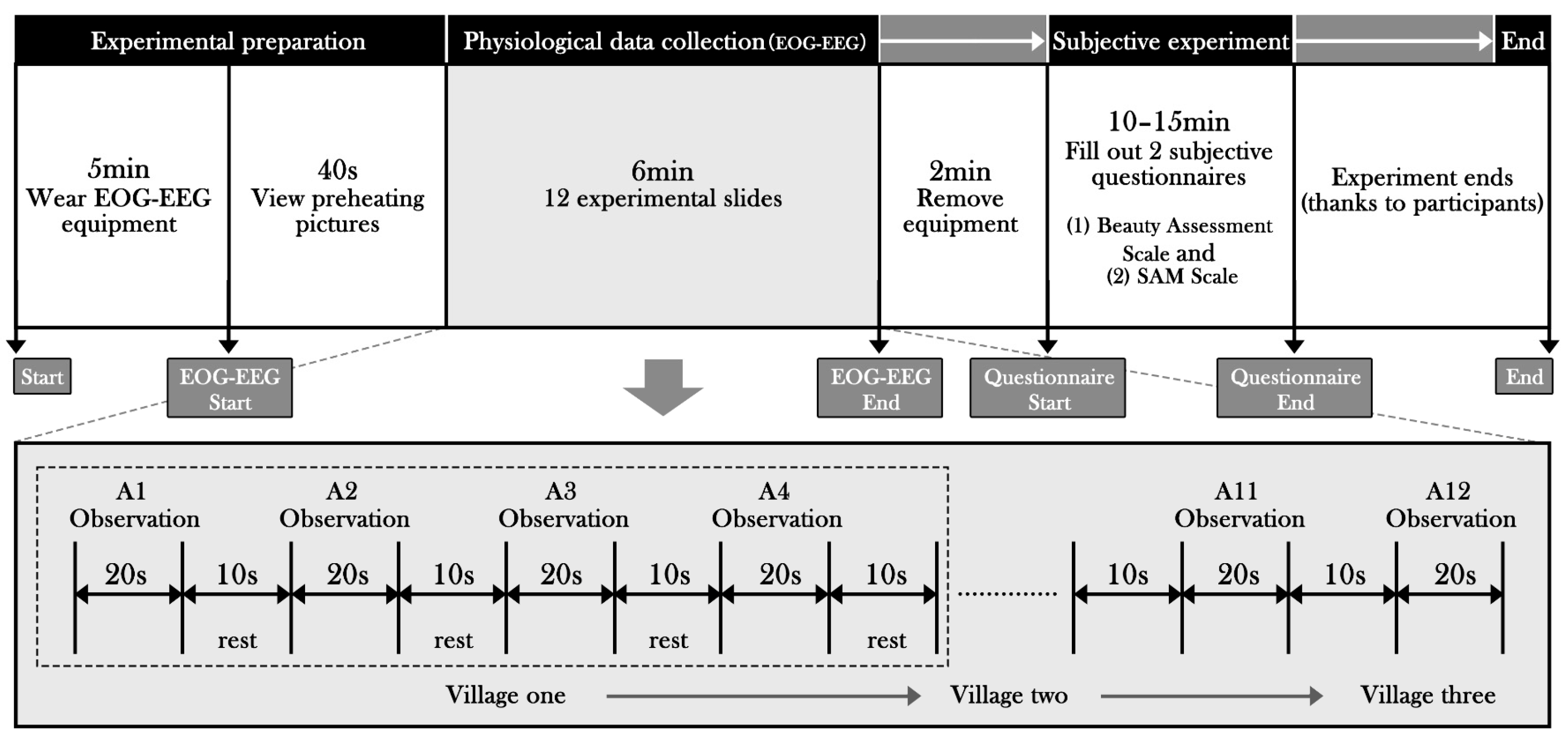
2.2.4. Experimental Procedures

The experiments were conducted individually in a controlled laboratory setting, adhering to a standardized procedure, with participants instructed to wash their scalp prior to the experiment to minimize impedance [63]. Initially, participants, equipped with the necessary sensors, were asked to complete a pretest involving eye movement and electrical brain stimulation by remaining seated and viewing four warm-up photos as directed by the experimenter. Upon meeting the pre-experiment standards, participants, under the experimenter’s guidance, proceeded to view a series of 12 stimulus photos (A1–A12) sequentially, following the stimulus presentation protocol of 20 s of viewing, followed by a 10 s rest period, to ensure the consistency of experimental variables. The collected EOG and EEG signals were transmitted and stored in a laptop via signal amplifiers. Throughout the experiment, efforts were made to maintain a constant environment, ensuring that only the stimuli presented on the monitor influenced the participant’s responses, thereby ensuring a high correlation between the results and the stimulus conditions. Upon completing the physiological portion of the experiment, participants rested briefly, removed the physiological sensors, and then filled out both the Beauty Assessment Scale and the SAM Scale questionnaires. After questionnaire completion, participants were thanked, and the experiment concluded (as shown in Figure 6). The total duration of the experiment was approximately 23–28 min.

2.3. Data Processing

2.3.1. Eye Movement Data Preprocessing

Following the experiment, raw eye-tracking data were processed using Pupil Player (Braincraft, Beijing, China) and eyeeso Studio 6.23 (Braincraft, Beijing, China) to ensure data integrity and consistency. Data segmentation, primarily conducted in Pupil Player, involved multiple steps, including blink removal, target area identification, and video cropping. The segmented data were then imported into eyeeso Studio for further analysis. Subsequent procedures included gaze statistics, definition and editing of Areas of Interest (AOIs), generation of attention heatmaps (as illustrated in Figure 7), and visualization of eye movement trajectories. The software extracted 31 specified signal parameters and exported them as CSV files. The hotspot map analysis algorithm calculates the aggregated Gaussian distribution of each fixation point on a given visual stimulus. Assuming a mean µ = 0, the standard deviation σ and the co-directional distribution are computed using the following Formulas (1):
f x , y = e x 2 + y 2 2 σ 2 2 π σ 2 , x , y [ s , s ]
The standard deviation σ is internally defined as σ = s/5. For each fixation, every element of the kernel template is scaled by a weight proportional to that fixation’s duration. These weighted kernels—anchored at their respective fixation coordinates—are then summed into an array representing stimulus intensity. Finally, the array is normalized, yielding stimulus magnitude and height maps (topographic maps).
Attention heatmaps employ a two-dimensional Gaussian kernel convolution to visually depict subjects’ attention distribution across the stimulus. Red denotes areas of concentrated focus, while yellow and green indicate lower attentiveness. From these maps, we observe the following:
(1) Architectural landscapes: All three villages exhibit focal fixation on discrete features—wall details in Xutun Village, landmark edifices in Yangquan Circle Village, and dispersed points of interest in Shabao Village—underscoring the visual salience of unique or intricate architectural elements.
(2) Water landscapes: Hotspots arise at feature boundaries or protrusions—the stream banks in Xutun Village, cliff faces along Yangquan Circle Village’s shore, and open water in Shabao Village—suggesting that contrasts between dynamic/static and smooth/abrupt forms guide gaze behavior.
(3) Vegetation landscapes: Attention clusters correspond to variations in color, stratification, and morphology—layered vegetation in Xutun Village, distinctive species in Yangquan Circle Village, and density fluctuations in Shabao Village—demonstrating that biodiversity and structural diversity capture visual interest.
(4) Road landscapes: Both linear pathways and discrete roadside elements shape eye trajectories—unique road alignments in Xutun Village, signage in Yangquan Circle Village, and surrounding objects in Shabao Village—highlighting the combined influence of spatial guidance and salient features on gaze patterns.

2.3.2. EEG Data Preprocessing

The EEG signals were preprocessed using the data analysis software Asalab 4.10.2 (ANT Neuro, Berlin, Germany), which included steps such as downsampling, re-referencing, and artifact removal. Asalab software decodes and converts the received electrical signals into visual representations, while simultaneously storing and analyzing them in the background for detailed monitoring and assessment of EEG signals. In clinical settings, the frequency-band energy ratio (FBER) is commonly utilized as a characteristic parameter to quantitatively assess changes in the basic rhythm of EEG signals [64]. In this study, the FBER value is referred to as the R-value. The R-value reflects the proportion of different waveforms across the EEG electrodes, which include eight points: Fz, Cz, Pz, F3, F4, Fpz, C3, and C4. As a crucial EEG characteristic parameter, the R-value can be used to evaluate the subject’s cerebral cortex preference and excitability in response to the rural visual landscape, based on its magnitude and variation. A total of eight EEG characteristics were derived. The frequency-band energy ratio (R-value) is calculated as follows in (2) and (3):
E a l l k = E j k j
R = E j k E a l l k
where j represents any electrode in Fz, Cz, Pz, F3, F4, Fpz, C3, and C4, E(j)(k) represents the power value of the electrode point, and Eall(k) represents the total power value of the eight electrode points.

2.3.3. Preprocessing of Scenic View Evaluation Data

The questionnaire, utilizing a Likert scale, explicitly instructs participants to interpret adjacent scores as representing equal psychological distances [65]. To facilitate the subsequent comprehensive analysis of physiological continuous variables (eye movement and EEG) within a unified dimension, statistical verification of isometric continuous variables was conducted. Initially, a data distribution test was performed using SPSS 24.0 (IBM, Armonk, NY, USA) on eight indicators, as shown in Table 1, revealing that the absolute values of skewness and kurtosis for all variables were less than 1, indicating an approximately symmetric distribution [66]. Subsequently, unidimensional verification through factor analysis yielded a Kaiser–Meyer–Olkin (KMO) value of 0.916 and a factor loading of 60.14%, confirming the suitability of the data for factor analysis and demonstrating strong unidimensional properties. This aligns with established practices in multimodal data fusion within the engineering domain [67].

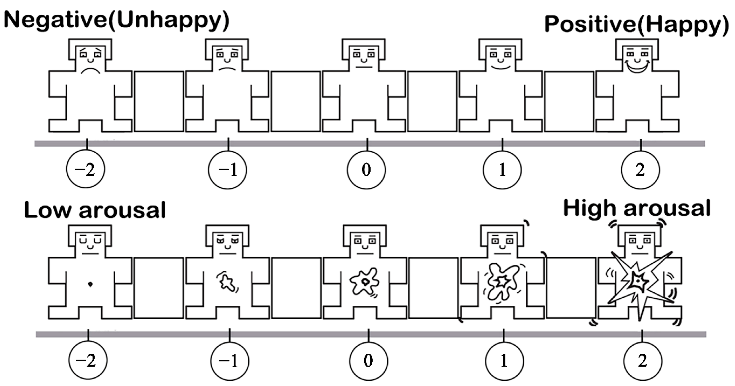
2.3.4. SAM Scale Data Preprocessing

The SAM questionnaire responses were classified at three granularity levels—binary, ternary, and five-category. In the binary schema, valence and arousal are dichotomized into two poles (“positive”/“negative” or “high arousal“/“low arousal”); for example, a participant’s sense of pleasure toward a rural architectural scene is tagged “1”, whereas perceptions of monotony are tagged “–1”, facilitating rapid screening of landscapes in need of renovation. The ternary schema introduces a neutral category “0” to capture ambivalent states; for instance, when participants neither favor nor dislike a given rural road scene, it is assigned “0”, supporting refined assessments that distinguish landscapes requiring optimization from those warranting preservation. The five-category schema further subdivides emotional intensity into “−2, −1, 0, 1, 2” (ranging from “extremely negative” to “extremely positive”), such as rating a sea of flowers as “2” and a dilapidated farmhouse as “−2”. Although theoretically more granular, this approach may suffer from sample-imbalance, degrading model performance. Accordingly, for the binary model, samples with valence/arousal “0” were excluded; values “−2” and “−1” were consolidated as negative/low “−1” and “1” and “2” as positive/high “1”. In the ternary model, “0” samples are retained as neutral for both valence and arousal.
After data processing, four incomplete entries were removed, resulting in a final valid dataset of 34 participants. This dataset comprises eye movement data (12,648 entries), EEG data (3264 entries), and beauty evaluation data (3264 entries), yielding a total of 19,176 data points.

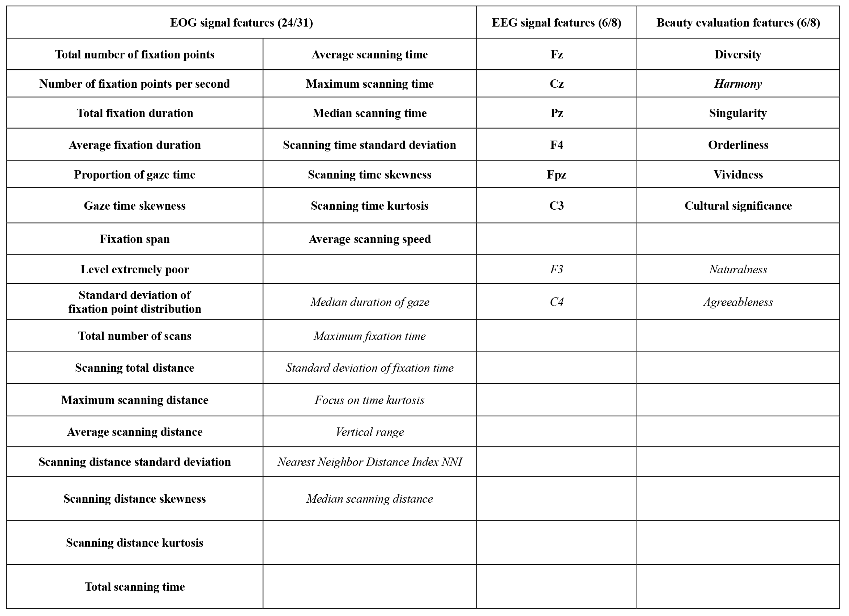
2.3.5. Feature Extraction and Reduction

To determine the number and validity of features, various software packages were employed to extract features from the physiological signals and Beauty Assessment Scale. This process yielded 31 eye movement signal features, 8 EEG features, and 8 beauty assessment features, for a total of 47 features. During the preprocessing stage, it was confirmed that the beauty assessment data could be comprehensively analyzed alongside the physiological continuous variables (eye movement and EEG). Consequently, data normalization was applied separately to both the beauty assessment and physiological data, standardizing dimensions and mitigating specific effects [68]. The calculation method is outlined in Formula (4) below:
z i = x i μ σ
where μ represents the mean and σ denotes the standard deviation, both calculated from the entire signal X, with xiX being the individual data points collected from a subject.
The standardization process was carried out independently for three distinct data types (eye movement, EEG, and beauty assessment). Subsequently, principal component analysis (PCA) was conducted on 47 signal features using SPSS 24.0 (IBM, Armonk, NY, USA) [69,70,71]. The results indicate that the Bartley sphere test is statistically significant (p < 0.01), with a Kaiser–Meyer–Olkin (KMO) value of 0.772, confirming the efficacy of PCA. The cumulative contribution rate of the extracted eigenvalues was found to be 90.775%; for details, please refer to Table A1 in the Appendix A. After calculating and comparing the weights of each feature, 36 features (depicted in Figure 8), which exhibited a strong correlation with mood, were selected.

2.4. Model Construction and Evaluation Methods

During data collection and processing (Section 2.1, Section 2.2 and Section 2.3), four visual landscape datasets from three villages were assembled, encompassing physiological signals (EEG, EOG) and subjective evaluations (Beauty Assessment and SAM Scales). By synchronizing data acquisition, standardizing preprocessing, and applying PCA for feature extraction, we harmonized physiological and subjective features within a unified dimensional space, ensuring data coherence and optimizing inputs for the subsequent sentiment classification model. Thereafter, SMOTE and Bayesian optimization were employed to enhance binary, ternary, and quinary classification performance—elevating accuracy, precision, recall, and F1 score—and thereby validating the coordinated integration of physiological data with subjective questionnaire metrics.

2.4.1. Build the Model

The rural visual landscape serves as a setting for the daily recreation of villagers, with spatial stimuli predominantly evoking positive or tranquil emotional responses. We observed that the samples labeled “−2” and “−1” in the valence and arousal datasets were significantly smaller than other samples, which resulted in poor recognition of negative emotions in the training model. To achieve a balanced class distribution, we employed the Synthetic Minority Over-sampling Technique (SMOTE) [72], utilizing k-nearest neighbor interpolation (k = 5, determined via grid search) to augment the number of samples in each minority class to match those of the majority class. Additionally, we implemented Bayesian optimization for hyperparameter tuning. Hyperparameter optimization plays a pivotal role in enhancing the performance of machine learning models by intelligently searching the parameter space to maximize the model’s generalization capacity. In this study, the HyperOpt Python 3.9 (Python Software Foundation, Wilmington, DE, USA) library [73,74] was used for hyperparameter tuning within the classifier element pool. Compared to traditional grid search and random search methods, this optimization strategy is particularly well suited for the multi-level classification system (binary, ternary, five-element classification) developed in this research. By defining the objective function as the weighted accuracy index of the test set (independently verified by villages), SMOTE effectively mitigated the potential risk of data leakage post-cross-validation [75]. Consequently, the classification robustness of the model was significantly enhanced in a few categories.
In classifier selection, we observed that single classifiers such as Logistic Regression (LR), Support Vector Machine (SVM), Decision Tree (DT), Artificial Neural Network (ANN), and Random Forest (RF) are commonly employed [76,77,78,79]. However, ensemble learning has been shown to yield superior predictive performance by aggregating the predictions from multiple models. Consequently, we utilized two single classifiers and two ensemble classifiers for model training. The single classifiers were LR-GD and DT, while the ensemble classifiers consisted of RF (Python 3.9) and XGBoost (Python 3.9).

2.4.2. Evaluation Methods

The confusion matrix, also referred to as the error matrix, is a visual tool primarily employed to compare the classification outcomes with the actual observed values, thereby providing a clear representation of the classification accuracy. The performance metrics of the classification model include accuracy, precision, recall, and the F1 score. By utilizing the confusion matrix, one can assess the misclassifications made by the model, facilitating subsequent adjustments to model parameters or data augmentation. The calculation methods are as follows (5)–(8):
A c c u r a c y = T P + T N T P + T N + F P + F N
P r e c i s i o n = T P T P + F P
R e c a l l = T P T P + F N
F 1 s c o r e = 2 × ( P r e c i s i o n × R e c a l l ) P r e c i s i o n + R e c a l l
where TP denotes the number of true positives in the positive category, FN represents the number of false negatives in the positive category, FP indicates the number of false positives in the negative category, and TN refers to the number of true negatives in the negative category.

3. Results

3.1. Impact of Feature Reduction on the Model

The PCA algorithm was employed to reduce the 47 extracted features to 36. However, while PCA effectively reduces the dimensionality of the independent variables, it does not clarify the significance of these variables in relation to the target variables. To assess whether the reduction in feature count positively impacts valence classification, we constructed binary and ternary classification models using both 47 and 36 signal features, respectively, with XGBoost and Random Forest as classifiers. The model performance results, before and after the reduction in valence and arousal features, are presented in Table 2 and Table 3.

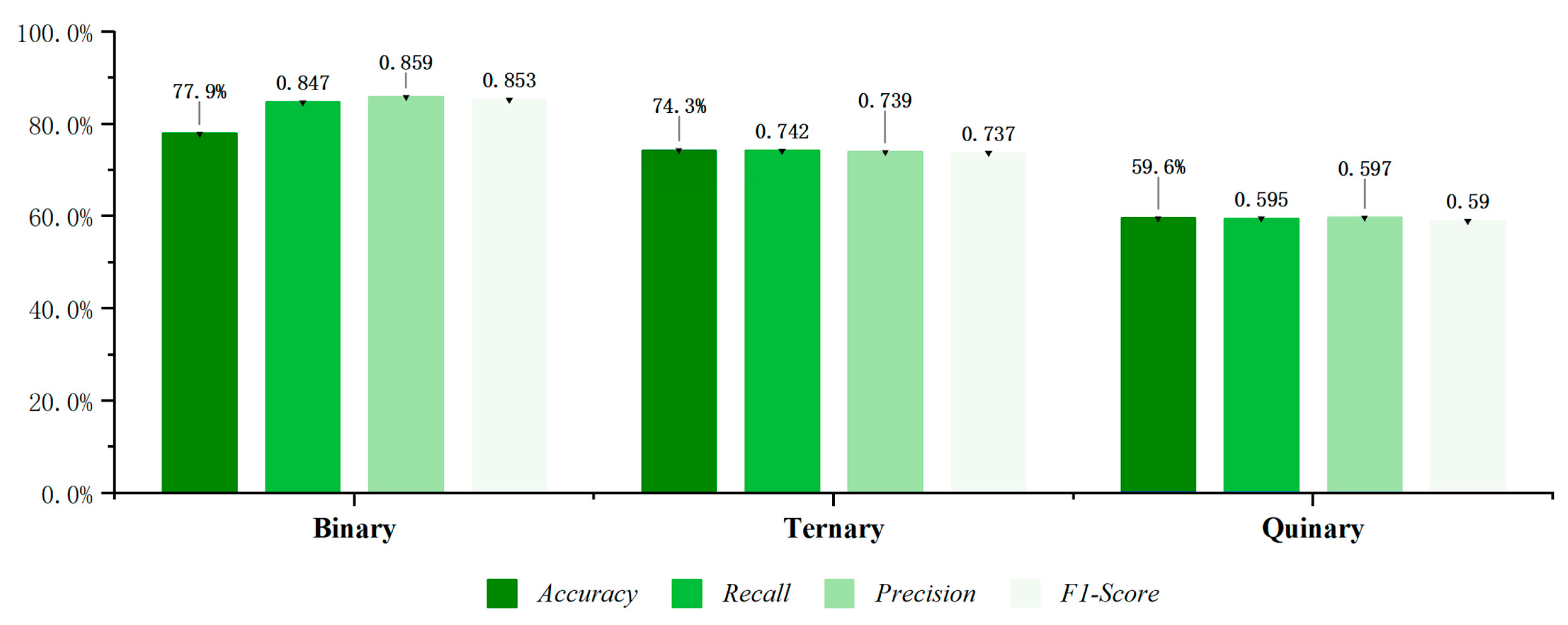
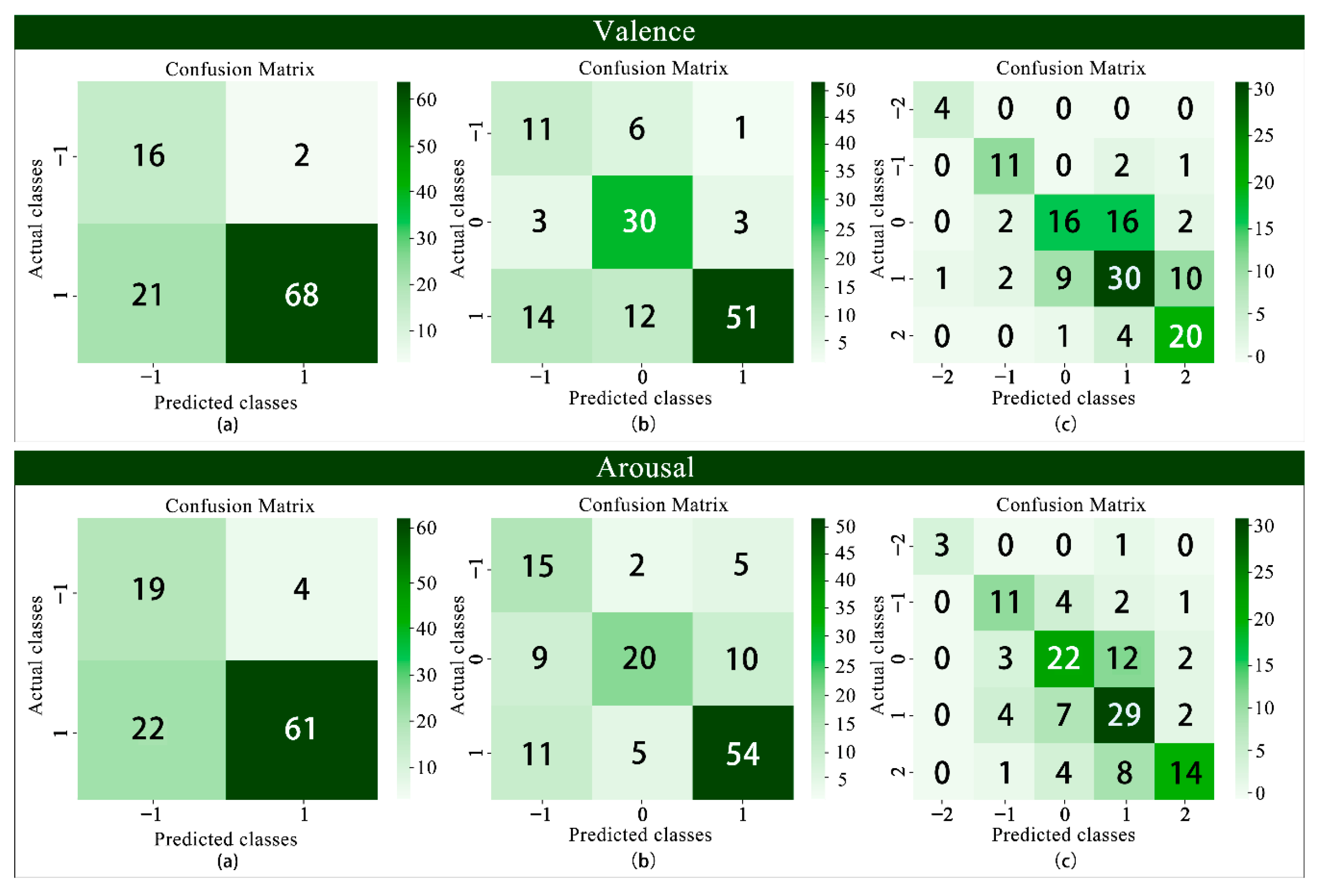
3.2. Model Classification Results and Performance Comparison

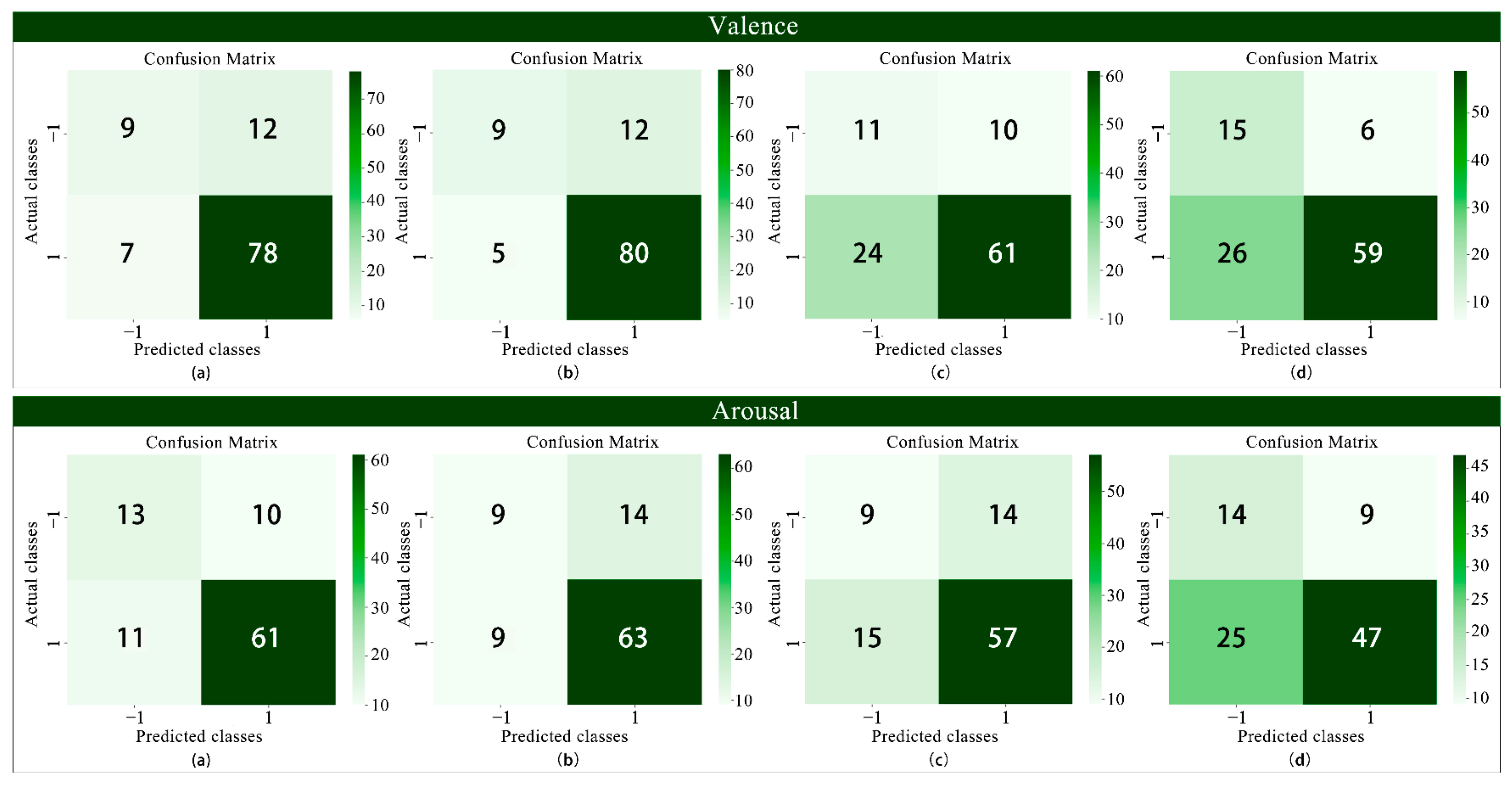
3.2.1. Binary Classification

Villages 1 and 2 were utilized as the training models, while Village 3 served as the test model. The training and test sets were randomly selected, and SMOTE along with Bayesian optimization were applied to enhance the model’s performance. In binary classification, the target variable values were “−1” and “1”, with 36 signal features as independent variables, and valence and arousal as the dependent variables. The model performance results are presented in Table 4 and Figure 9.
The binary classification results indicate that the model’s recognition accuracy for emotional pleasure, based on XGBoost and RF, surpasses 80%. For emotional arousal, both the XGBoost- and RF-based models achieve recognition accuracy rates exceeding 75%, demonstrating robust classification performance. These findings further suggest that both models are effective in assessing the emotional quality of rural visual landscapes.

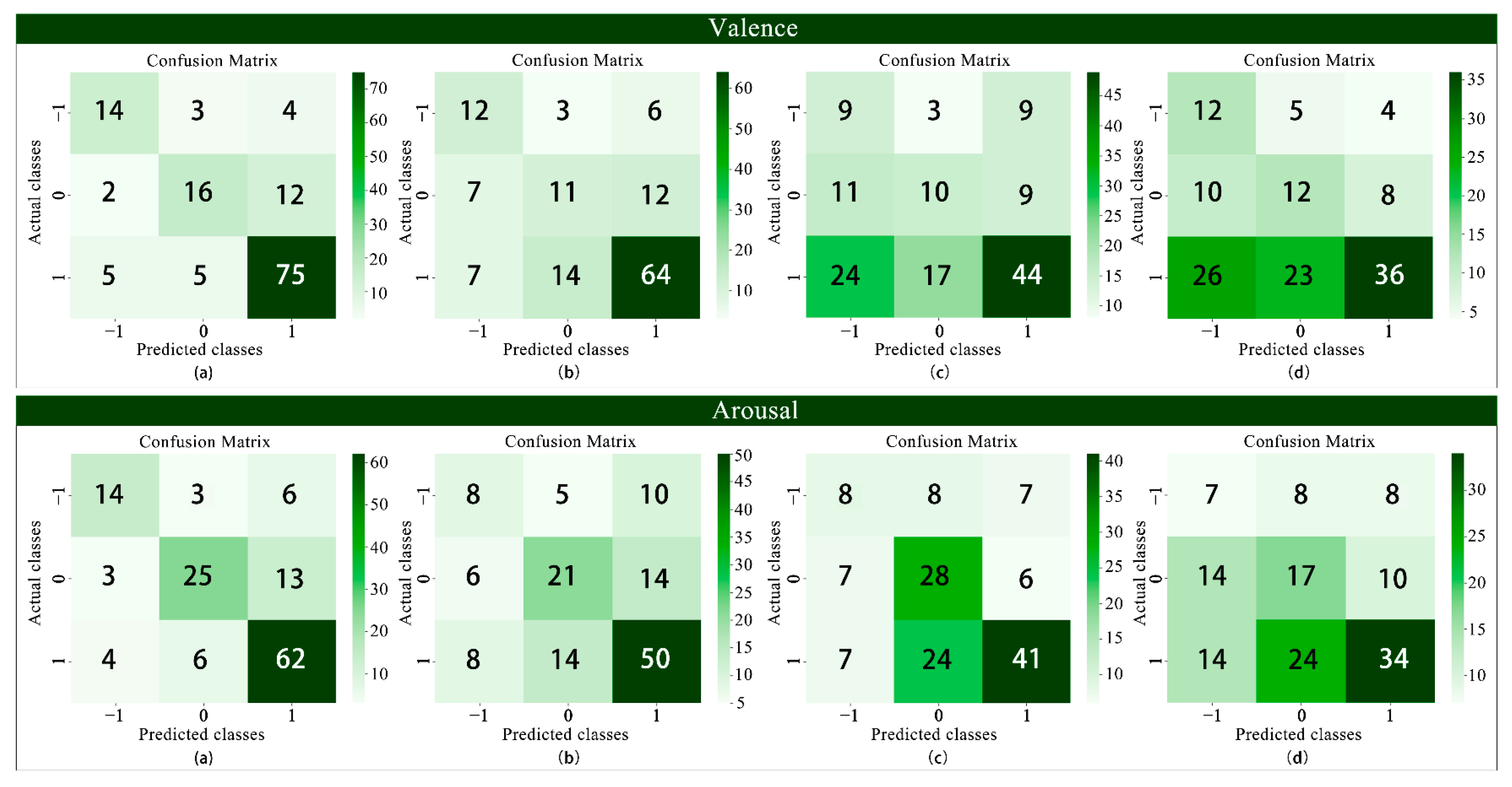
3.2.2. Ternary Classification

The target variable values for triadic classification are “−1”, “0”, and “1”, with all valid sample data utilized for model training and testing, incorporating SMOTE and Bayesian optimization. Following model evaluation, we obtained the classification accuracy for each performance indicator, as presented in Table 5 and Figure 10.
Through the observation of emotional pleasure and arousal, the XGBoost-based model demonstrated higher performance index values, achieving recognition accuracies of 77.2% and 74.3%, respectively. In comparison, the RF model’s recognition accuracies were 64.0% and 58.1%, respectively. These results indicate that the XGBoost model is more effective in evaluating the emotional quality of rural visual landscapes.

3.2.3. Five-Element Classification

The target variable values for the five classifications are “−2, −1, 0, 1, 2”, with all valid sample data utilized for model construction, incorporating SMOTE and Bayesian optimization. After evaluating these models, we obtained the classification accuracy, precision, recall, and F1 scores for each category, as presented in Table 6 and Figure 11.
The results of the five classifications indicate that the XGBoost model exhibits the best classification performance in emotional pleasure, although its accuracy is only 64.0%. In terms of emotional arousal, the XGBoost model demonstrates superior classification performance; however, the accuracy of all four models remains below 60%. Therefore, in practical terms, none of these four models can adequately address the emotional quality assessment of rural visual landscapes in five-element classification.

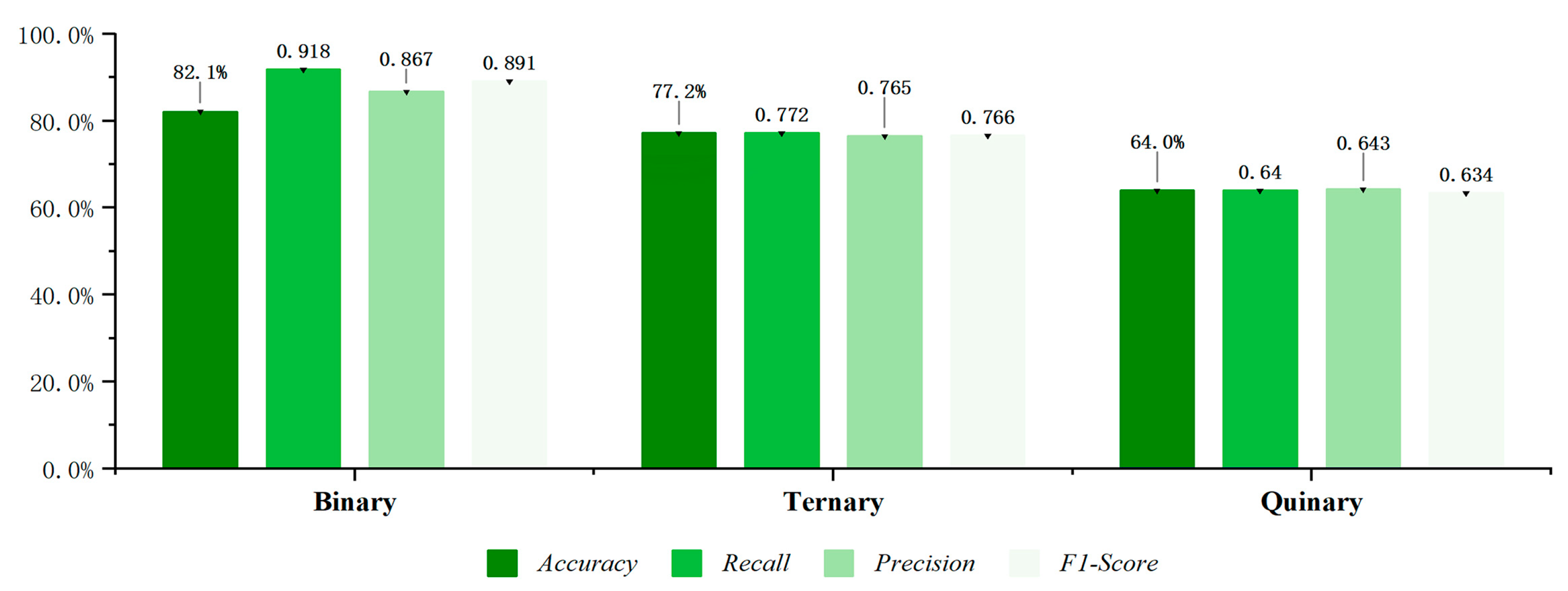
3.2.4. Comparison of Optimal Classification Performance of Models

Figure 12 and Figure 13 present a comparison of the four indices for the binary, ternary, and quintuple classification models of emotional valence and optimal arousal performance (XGBoost), respectively. The results reveal a progressive decline in classification ability, with a significant decrease observed in the five-element classification. The binary and ternary classification models, however, are shown to meet the practical requirements.

3.2.5. External Validation

In addition to internal testing and performance benchmarking, the model underwent external validation. A new dataset was constructed using the four preheating images presented prior to the formal experiment and was input into the XGBoost classification model, which demonstrated relatively high accuracy. This process aimed to assess the model’s effectiveness in predicting the emotional quality of novel spatial stimuli. The model generated outputs in binary, ternary, and five-class classifications. By comparing these predicted classifications with the ground truth labels, we derived classification accuracy and confusion matrices, as presented in Table 7 and Figure 14.
The results indicate that the highest external validation accuracy was achieved in the binary classification, reaching 78.50%, followed by the ternary and five-class models with accuracies of 70.23% and 61.83%, respectively. Additionally, the classification accuracy for valence consistently outperformed that for arousal. The ternary confusion matrix reveals that samples labeled with a valence of −1 were more frequently misclassified than those in other categories. In the five-class system, due to the limited number of samples labeled as −2, the classification performance for labels 0 and 1 was comparatively more accurate.

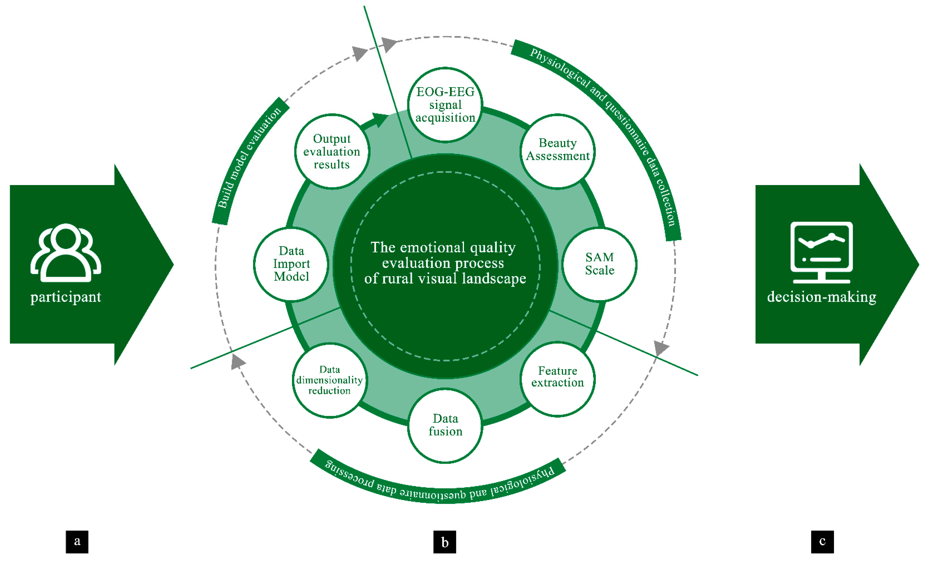
3.3. Model Usage Process

This training model is designed to assess the quality of rural visual landscapes in practical settings. Consequently, we sought to establish a process for evaluating the emotional quality of rural visual landscapes using multi-source data (as illustrated in Figure 15). The process encompasses the following steps: First, we defined the experimental route and divided it into several segments. Next, we invited participants to engage in the study and sign a consent form. During the signal collection phase, we gathered both physiological and subjective data from participants while they viewed the images. After feature extraction, fusion, and dimensionality reduction, the processed data were input into the classification model. Based on the emotion score derived from the model, areas with a positive emotional value will be preserved, while spaces with a negative emotional value will undergo renovation.

4. Discussion

This study integrates eye movement, EEG, and a subjective beauty questionnaire to construct and evaluate a multi-source affective computing model tailored for assessing rural visual landscapes. Model performance was optimized through feature selection, SMOTE, Bayesian optimization, and ensemble classification. Generalizability was evaluated via external validation, and the normality assumption underlying the subjective aesthetic questionnaire was empirically examined.

4.1. Collaborative Classification of Multimodal and Subjective Data

As a crucial method for assessing visual quality in human–environment interactions, emotion calculation is primarily conducted through single modalities, such as GIS, questionnaires, and physiological sensors. Although multimodal sensors, such as eye movement + EEG and skin electrocardiogram + ECG, have been employed, subjective questionnaires are rarely used as independent variables. Consequently, this study integrates subjective questionnaires (beauty assessment) with objective physiological signals (eye movement, EEG) to create a multi-source dataset encompassing eight semantic variables (e.g., naturalness, diversity, coordination). The symmetric distribution test (with absolute values of skewness and kurtosis both < 1) and unidimensional test (KMO = 0.916, factor load 60.14%), as described in Shing-On Leung’s study [66], confirm that the Li Keert scale satisfies the conditions for continuous variable analysis in emotion questionnaires, thus mitigating the potential confounding effects of multi-dimensionality on model fusion. In model validation, robust fusion of multi-source features is achieved through ensemble learning. For instance, in the triadic classification task, the model combining subjective questionnaire and eye movement data achieved accuracy rates of 77.2% and 74.3% for valence and arousal emotion classification, respectively. This performance exceeds the accuracy of valence (76.1%) and arousal (67.7%) in triadic classification using the fusion of eye movement and EEG by Mohammad Soleymani et al. Additionally, the accuracy surpasses that of Wei-Bang Jiang et al. [30] and Kazuhiko Takahashi [79], who utilized eye movement and EEG as standalone modalities for emotion calculation, thereby confirming the efficacy of multimodal and subjective data collaboration in emotion classification.

4.2. Classifier Generalization Verification

In this study, Village 1 and Village 2 were used for training, while Village 3 served as the validation set. The performance of classifiers across binary, ternary, and quintuple tasks (XGBoost, RF, DT, LR-GD) was systematically compared. To enhance the comparability and practical applicability of model validation, PCA feature extraction was applied consistently across classifiers. After reducing the number of features from 47 to 36, the model’s recognition accuracy increased by an average of 5.2% for valence and 6.4% for arousal, with other performance metrics also improving. These findings demonstrate that the PCA algorithm effectively reduces data redundancy and noise, thereby enhancing model classification capabilities. However, obtaining a sufficient number of meaningful features remains a challenge, one that requires further academic consensus through extensive experimentation. Furthermore, the integration of SMOTE and Bayesian optimization techniques was employed to compare the performance of integrated versus single classifiers. The results showed that, for valence, the highest binary classification accuracy was 84%, ternary classification accuracy was 77.2%, and quintuple classification accuracy was 64%. For arousal, the highest accuracy was 77.9% for binary classification, 74.3% for ternary classification, and 59.6% for quintuple classification. Notably, the integrated classifiers exhibited superior performance in binary and ternary classification, with higher performance metrics, while the quintuple classification accuracy was notably lower—64% for both valence and arousal—compared to 79% achieved by Kalimeri and Saitis [80]. This discrepancy is attributed to the varied emotional responses elicited by image-based experiments versus real-world scenarios [81], an issue that will be further investigated through virtual scene construction or field experiments in the future. Furthermore, the proposed model underwent external validation to address the limitations associated with deriving both training and validation data from the same image set. When new data were introduced into the model, a decline in performance was observed, with average decreases of 4.25% in valence classification accuracy and 3.31% in arousal. These findings underscore the necessity of incorporating external validation, as relying solely on a unified dataset is insufficient for robust classification research. Additionally, it was observed that the average accuracy for valence exceeded that of arousal by 7.4% across binary, ternary, and quintuple classifications, supporting the weak V-shaped relationship and individual differences identified by Kuppens et al. [82] in their analysis of average relationships.

4.3. Enrich Sustainable Assessment Methods

Building on the analysis above, this study has been validated by constructing a multi-source emotion model that integrates eye movement, EEG, and landscape beauty questionnaires into a unified framework. This approach enriches the interdisciplinary methodology for assessing rural landscape sustainability. In practical terms, the model provides innovative solutions to address the three major challenges in rural revitalization, as outlined in Section 3.3 First, by establishing the spatial coupling relationship between eye movement, EEG, beauty assessment questionnaires, and the SAM emotion scale, we can accurately identify traditional villages that require protection, thus preventing the destruction of cultural heritage caused by the “largescale demolition and construction” transformation. Second, dynamic monitoring, based on an emotional feedback database, enables the establishment of a tiered update mechanism—comprising “negative spatial early warning, moderate intervention, and positive maintenance”—that overcomes time-domain constraints and facilitates real-time monitoring of emotional responses to rural landscape designs. Third, the model can be seamlessly integrated with GIS systems to transcend the limitations of point-based analysis, enhancing the ecological perception of tourists’ experiences. Finally, the visual emotional responses are translated into quantifiable landscape indicators through the affective computing model, enabling rural landscape designers to better contribute to SDG 11.7 (providing inclusive green public spaces) through the quantitative insights offered by the multi-source affective model.

4.4. Limitations and Challenges

Although this study has established a foundational framework for multi-source sentiment computing in rural visual landscapes, several notable limitations remain. First, the geographic concentration on three villages in Dalian constrains the generalizability of cultural and ecological insights to other regions. Future research should therefore focus on diversifying application contexts and expanding the geographical scope. Second, the participant pool—comprising exclusively students and teachers—exhibited a degree of homogeneity. Subsequent studies should include a broader demographic spectrum, such as rural residents and tourists, to more accurately evaluate the model’s applicability across different user groups and to strengthen the generalizability of the findings. Finally, the current experiment employed two-dimensional images as stimuli, limiting emotional extraction to flat visual environments. To improve the ecological validity of emotional assessments, future investigations should consider developing a multimodal virtual or augmented reality platform that incorporates environmental variables such as seasonal transitions and dynamic lighting conditions. This would foster more immersive experimental settings and enable dynamic, adaptable evaluations. Collectively, these advancements will offer critical technical support for refining the emotional assessment framework and enhancing its applicability in complex real-world environments.

5. Conclusions

Despite the aforementioned limitations, the rural visual landscape evaluation based on multi-source emotion computing effectively meets the decision-making requirements for rural landscape renewal through binary and ternary emotional assessments. Whether utilizing multimodal physiological sensors or various questionnaire evaluations, assessing rural visual landscapes across different regions, styles, and functions has been a contentious issue in rural revitalization. This study primarily focuses on enhancing the adaptability and classification performance of the proposed model. To achieve a more versatile model, data were collected from four distinct landscape types across three villages, ensuring the diversity of spatial data. Furthermore, efficient feature reduction, the SMOTE algorithm, Bayesian optimization, and ensemble learning techniques were employed to enhance the classification accuracy of the model. This paper also compares the performance of binary, ternary, and five-element classification models. Ultimately, accuracy comparisons reveal that the binary and ternary classification models outperform the five-element model in fulfilling practical requirements.
In future research, we aim to explore long-term emotional assessment, dynamic evaluation, and the integration of virtual and real-world emotional quality evaluations. By leveraging multi-source signal extraction and advanced machine learning technologies, we seek to continuously enhance the performance of the multi-source emotion computing model, thereby providing technical support for the development of rural visual landscapes.

Author Contributions

Conceptualization, X.Z. and L.L.; methodology, X.Z. and R.L.; software, X.Z. and Z.W.; validation, X.Z. and L.L.; formal analysis, X.Z. and L.L.; investigation, X.Z. and X.G.; resources, X.G. and R.L.; data curation, X.Z.; writing—original draft preparation, X.Z.; writing—review and editing, X.Z., L.L., X.G., R.L. and Z.W.; visualization, X.Z.; supervision, X.Z., L.L., X.G. and R.L.; project administration, X.Z., L.L. and X.G.; funding acquisition, X.G. and R.L. All authors have read and agreed to the published version of the manuscript.

Funding

Humanities and Social Science Fund of Chinese Ministry of Education (Number: 21YJC760022), and Supported by Guizhou Provincial Science and Technology Projects, number [2023] general project 116, Liaoning Province Social Science Federation project (Number: 2025lslybwzzkt-049), and Ministry of Education industry-university cooperative education project (Number: 231107615030255).

Institutional Review Board Statement

This study was conducted in accordance with the Declaration of Helsinki, and approved by the Institutional Ethics Committee of DALIAN POLYTECHNIC UNIVERSITY (protocol code 20241115 and date of 15 November 2024).

Informed Consent Statement

Informed consent was obtained from all subjects involved in the study.

Data Availability Statement

The data that support this study are available from the authors upon reasonable request.

Acknowledgments

We thank all the study participants in this study.

Conflicts of Interest

The authors declare no conflicts of interest.

Abbreviations

The following abbreviations are used in this manuscript:
EOGelectrooculogram
EEGelectroencephalogram
SAMSelf-assessment
XGBoosteXtreme Gradient Boosting
RFRandom Forest
DTDecision Tree
LR-GDLogistic Regression–Gradient Descent

Appendix A

Table A1. Principal component contribution rate and cumulative contribution rate.
ComponentEigenvalueContribution Rate *Cumulative Contribution Rate *
F18.23517.52217.522
F26.31713.44130.963
F34.72610.05641.019
F44.2819.10950.128
F54.0098.52958.657
F62.0574.37663.033
F71.8413.91866.951
F81.2542.66869.618
F91.1382.42272.040
F101.0802.29774.338
F110.9902.10676.444
F120.9532.02878.472
F130.8271.76080.231
F140.7801.65981.890
F150.7591.61683.506
F160.6721.42984.935
F170.6481.37886.313
F180.6021.28187.594
F190.5331.13388.727
F200.5181.10289.829
F210.4440.94590.775
* The unit of these data is %.

References

  1. Kaplan, A.; Taskin, T.; Onenc, A. Assessing the Visual Quality of Rural and Urban-fringed Landscapes Surrounding Livestock Farms. Biosyst. Eng. 2006, 95, 437–448. [Google Scholar] [CrossRef]
  2. Yin, C.; Zhao, W.; Pereira, P. Ecosystem Restoration along the “Pattern-Process-service-sustainability” Path for Achieving Land Degradation Neutrality. Landsc. Urban Plan. 2025, 253, 105227. [Google Scholar] [CrossRef]
  3. Plieninger, T.; Dijks, S.; Oteros-Rozas, E.; Bieling, C. Assessing, Mapping, and Quantifying Cultural Ecosystem Services at Community Level. Land Use Policy 2013, 33, 118–129. [Google Scholar] [CrossRef]
  4. Sarma, P.; Barma, S. Review on Stimuli Presentation for Affect Analysis Based on EEG. IEEE Access 2020, 8, 51991–52009. [Google Scholar] [CrossRef]
  5. Engelen, T.; Buot, A.; Grezes, J.; Tallon-Baudry, C. Whose Emotion is It? Perspective Matters to Understand Brain-Body Interactions in Emotions. Neuroimage 2023, 268, 119867. [Google Scholar] [CrossRef]
  6. Wang, Y.; Song, W.; Tao, W.; Liotta, A.; Yang, D.; Li, X.; Gao, S.; Sun, Y.; Ge, W.; Zhang, W.; et al. A Systematic Review on Affective Computing: Emotion Models, Databases, and Recent Advances. Inf. Fusion 2022, 83, 19–52. [Google Scholar] [CrossRef]
  7. Benssassi, E.M.; Ye, J. Investigating Multisensory Integration in Emotion Recognition Through Bio-Inspired Computational Models. IEEE Trans. Affect. Comput. 2021, 14, 906–918. [Google Scholar] [CrossRef]
  8. Ayata, D.E.; Yaslan, Y.; Kamasak, M.E. Emotion Recognition from Multimodal Physiological Signals for Emotion Aware Healthcare Systems. J. Med. Biol. Eng. 2020, 40, 149–157. [Google Scholar] [CrossRef]
  9. Esposito, A.; Esposito, A.M.; Vogel, C. Needs and Challenges in Human Computer Interaction for Processing Social Emotional Information. Pattern Recognit. Lett. 2015, 66, 41–51. [Google Scholar] [CrossRef]
  10. Naqvi, N.; Shiv, B.; Bechara, A. The Role of Emotion in Decision Making. Curr. Dir. Psychol. Sci. 2006, 15, 260–264. [Google Scholar] [CrossRef]
  11. Picard, R.W.; Vyzas, E.; Healey, J. Toward Machine Emotional Intelligence: Analysis of Affective Physiological State. IEEE Trans. Pattern Anal. Mach. Intell. 2001, 23, 1175–1191. [Google Scholar] [CrossRef]
  12. Pace, R.K.; Barry, R. Quick Computation of Spatial Autoregressive Estimators. Geogr. Anal. 1997, 29, 232–247. [Google Scholar] [CrossRef]
  13. Fleckenstein, K.S. Defining Affect in Relation to Cognition: A Response to Susan McLeod. J. Adv. Compos. 1991, 11, 447–453. [Google Scholar]
  14. Yadegaridehkordi, E.; Noor, N.F.B.M.; Ayub, M.N.B.; Affal, H.B.; Hussin, N.B. Affective Computing in Education: A Systematic Review and Future Research. Comput. Educ. 2019, 142, 103649. [Google Scholar] [CrossRef]
  15. Liberati, G.; Veit, R.; Kim, S.; Birbaumer, N.; Von Arnim, C.; Jenner, A.; Lulé, D.; Ludolph, A.C.; Raffone, A.; Belardinelli, M.O.; et al. Development of a Binary Fmri-Bci for Alzheimer Patients: A Semantic Conditioning Paradigm Using Affective Unconditioned Stimuli. In Proceedings of the 2013 Humaine Association Conference on Affective Computing and Intelligent Interaction, Geneva, Switzerland, 2–5 September 2013; pp. 838–842. [Google Scholar] [CrossRef]
  16. Pei, G.; Li, T. A Literature Review of EEG-Based Affective Computing in Marketing. Front. Psychol. 2021, 12, 602843. [Google Scholar] [CrossRef]
  17. Healey, J.A.; Picard, R.W. Detecting Stress During Real-World Driving Tasks Using Physiological Sensors. IEEE Trans. Intell. Transp. Syst. 2005, 6, 156–166. [Google Scholar] [CrossRef]
  18. Balazs, J.A.; Velasquez, J.D. Opinion Mining and Information Fusion: A Survey. Inf. Fusion 2016, 27, 95–110. [Google Scholar] [CrossRef]
  19. Gómez, L.M.; Cáceres, M.N. Applying Data Mining for Sentiment Analysis in Music. In Proceedings of the Advances in Intelligent Systems and Computing Trends in Cyber-Physical Multi-Agent Systems the Paams Collection—15th International Conference, Paams 2017, Porto, Portugal, 21–23 June 2017; pp. 198–205. [Google Scholar] [CrossRef]
  20. Ducange, P.; Fazzolari, M.; Petrocchi, M.; Vecchio, M. An Effective Decision Support System for Social Media Listening Based on Cross-Source Sentiment Analysis Models. Eng. Appl. Artif. Intell. 2018, 78, 71–85. [Google Scholar] [CrossRef]
  21. Maria, E.; Matthias, L.; Sten, H. Emotion Recognition from Physiological Signal Analysis: A Review. Electron. Notes Theor. Comput. Sci. 2019, 343, 35–55. [Google Scholar] [CrossRef]
  22. Kessous, L.; Castellano, G.; Caridakis, G. Multimodal Emotion Recognition in Speech-Based Interaction Using Facial Expression, Body Gesture and Acoustic Analysis. J. Multimodal User Interfaces 2009, 3, 33–48. [Google Scholar] [CrossRef]
  23. Poria, S.; Cambria, E.; Gelbukh, A. Aspect Extraction for Opinion Mining with a Deep Convolutional Neural Network. Knowl.-Based Syst. 2016, 108, 42–49. [Google Scholar] [CrossRef]
  24. Cambria, E.; Das, D.; Bandyopadhyay, S.; Feraco, A. Affective Computing and Sentiment Analysis. In A Practical Guide to Sentiment Analysis; Springer: Berlin/Heidelberg, Germany, 2017. [Google Scholar] [CrossRef]
  25. Cambria, E.; Speer, R.; Havasi, C.; Hussain, A. Senticnet: A Publicly Available Semantic Resource for Opinion Mining. In AAAI Fall Symposium Commonsense Knowledge; AAAI Press: Menlo Park, CA, USA, 2010. [Google Scholar]
  26. Poria, S.; Cambria, E.; Bajpai, R.; Hussain, A. A Review of Affective Computing: From Unimodal Analysis to Multimodal Fusion. Inf. Fusion 2017, 37, 98–125. [Google Scholar] [CrossRef]
  27. Munezero, M.; Montero, C.S.; Sutinen, E.; Pajunen, J. Are They Different? Affect, Feeling, Emotion, Sentiment, and Opinion Detection in Text. IEEE T Affect. Comput. 2014, 5, 101–111. [Google Scholar] [CrossRef]
  28. Reilly, R.B.; Lee, T.C. II.3. Electrograms (ECG, EEG, EMG, EOG). Stud. Health Technol. Inform. 2010, 152, 90–108. [Google Scholar] [PubMed]
  29. Du, G.; Zeng, Y.; Su, K.; Li, C.; Wang, X.; Teng, S.; Li, D.; Liu, P.X. A Novel Emotion-Aware Method Based on the Fusion of Textual Description of Speech, Body Movements, and Facial Expressions. IEEE Trans. Instrum. Meas. 2022, 71, 5022816. [Google Scholar] [CrossRef]
  30. Jiang, W.; Liu, X.; Zheng, W.; Lu, B. SEED-VII: A Multimodal Dataset of Six Basic Emotions with Continuous Labels for Emotion Recognition. IEEE Trans. Affect. Comput. 2024, 1–16. [Google Scholar] [CrossRef]
  31. Alarcao, S.M.; Fonseca, M.J. Emotions Recognition Using EEG Signals: A Survey. IEEE Trans. Affect. Comput. 2019, 10, 374–393. [Google Scholar] [CrossRef]
  32. Zheng, W.; Lu, B. Investigating Critical Frequency Bands and Channels for EEG-Based Emotion Recognition with Deep Neural Networks. IEEE Trans. Auton. Ment. Dev. 2015, 7, 162–175. [Google Scholar] [CrossRef]
  33. Zheng, W.; Liu, W.; Lu, Y.; Lu, B.-L.; Cichocki, A. EmotionMeter: A Multimodal Framework for Recognizing Human Emotions. IEEE Trans. Cybern. 2018, 49, 1110–1122. [Google Scholar] [CrossRef]
  34. Soleymani, M.; Lichtenauer, J.; Pun, T.; Pantic, M. A Multimodal Database for Affect Recognition and Implicit Tagging. IEEE Trans. Affect. Comput. 2011, 3, 42–55. [Google Scholar] [CrossRef]
  35. Jafari, M.; Shoeibi, A.; Khodatars, M.; Bagherzadeh, S.; Shalbaf, A.; García, D.L.; Gorriz, J.M.; Acharya, U.R. Emotion Recognition in EEG Signals Using Deep Learning Methods: A Review. Comput. Biol. Med. 2023, 165, 107450. [Google Scholar] [CrossRef]
  36. Doma, V.; Pirouz, M. A Comparative Analysis of Machine Learning Methods for Emotion Recognition Using EEG and Peripheral Physiological Signals. J. Big Data 2023, 165, 18. [Google Scholar] [CrossRef]
  37. Li, R.; Yuizono, T.; Li, X. Affective Computing of Multi-Type Urban Public Spaces to Analyze Emotional Quality Using Ensemble Learning-Based Classification of Multi-Sensor Data. PLoS ONE 2022, 17, e0269176. [Google Scholar] [CrossRef] [PubMed]
  38. Verma, G.K.; Tiwary, U.S. Multimodal fusion framework: A multiresolution approach for emotion classification and recognition from physiological signals. Neuroimage 2014, 102, 162–172. [Google Scholar] [CrossRef] [PubMed]
  39. Triantafyllopoulos, A.; Schuller, B.W.; Iymen, G.; Sezgin, M.; He, X.; Yang, Z.; Tzirakis, P.; Liu, S.; Mertes, S.; André, E.; et al. An Overview of Affective Speech Synthesis and Conversion in the Deep Learning Era. Proc. IEEE 2023, 111, 1355–1381. [Google Scholar] [CrossRef]
  40. Heredia, B.; Khoshgoftaar, T.M.; Prusa, J.D.; Crawford, M. Integrating Multiple Data Sources to Enhance Sentiment Prediction. In Proceedings of the IEEE Conference Proceedings, Las Vegas, NV, USA, 7–10 December 2016. [Google Scholar] [CrossRef]
  41. Li, F.; Lv, Y.; Zhu, Q.; Lin, X. Research of Food Safety Event Detection Based on Multiple Data Sources. In Proceedings of the 2015 International Conference on Cloud Computing and Big Data (CCBD), Shanghai, China, 4–6 November 2015; pp. 213–216. [Google Scholar] [CrossRef]
  42. Mauro, A.; Antonio, S. Agricultural Heritage Systems and Agrobiodiversity. Biodivers. Conserv. 2022, 31, 2231–2241. [Google Scholar] [CrossRef]
  43. Arriaza, M.; Canas-Ortega, J.F.; Canas-Madueno, J.A.; Ruiz-Aviles, P. Assessing the Visual Quality of Rural Landscapes. Landsc. Urban Plan. 2003, 69, 115–125. [Google Scholar] [CrossRef]
  44. Howley, P. Landscape Aesthetics: Assessing the General Publics’ Preferences Towards Rural Landscapes. Ecol. Econ. 2011, 72, 161–169. [Google Scholar] [CrossRef]
  45. Misthos, L.; Krassanakis, V.; Merlemis, N.; Kesidis, A.L. Modeling the Visual Landscape: A Review on Approaches, Methods and Techniques. Sensors 2023, 23, 8135. [Google Scholar] [CrossRef]
  46. Swetnam, R.D.; Harrison-Curran, S.K.; Smith, G.R. Quantifying Visual Landscape Quality in Rural Wales: A GIS-enabled Method for Extensive Monitoring of a Valued Cultural Ecosystem Service. Ecosyst. Serv. 2016, 26, 451–464. [Google Scholar] [CrossRef]
  47. Criado, M.; Martinez-Grana, A.; Santos-Frances, F.; Merchán, L. Landscape Evaluation As a Complementary Tool in Environmental Assessment. Study Case in Urban Areas: Salamanca (Spain). Sustainability 2020, 12, 6395. [Google Scholar] [CrossRef]
  48. Yao, X.; Sun, Y. Using a Public Preference Questionnaire and Eye Movement Heat Maps to Identify the Visual Quality of Rural Landscapes in Southwestern Guizhou, China. Land 2024, 13, 707. [Google Scholar] [CrossRef]
  49. Zhang, X.; Xiong, X.; Chi, M.; Yang, S.; Liu, L. Research on Visual Quality Assessment and Landscape Elements Influence Mechanism of Rural Greenways. Ecol. Indic. 2024, 160, 111844. [Google Scholar] [CrossRef]
  50. Liang, T.; Peng, S. Using Analytic Hierarchy Process to Examine the Success Factors of Autonomous Landscape Development in Rural Communities. Sustainability 2017, 9, 729. [Google Scholar] [CrossRef]
  51. Cloquell-Ballester, V.; Torres-Sibille, A.D.C.; Cloquell-Ballester, V.; Santamarina-Siurana, M.C. Human Alteration of the Rural Landscape: Variations in Visual Perception. Environ. Impact Assess. Rev. 2011, 32, 50–60. [Google Scholar] [CrossRef]
  52. Ding, N.; Zhong, Y.; Li, J.; Xiao, Q.; Zhang, S.; Xia, H. Visual Preference of Plant Features in Different Living Environments Using Eye Tracking and EEG. PLoS ONE 2022, 17, e0279596. [Google Scholar] [CrossRef] [PubMed]
  53. Ye, F.; Yin, M.; Cao, L.; Sun, S.; Wang, X. Predicting Emotional Experiences Through Eye-Tracking: A Study of Tourists’ Responses to Traditional Village Landscapes. Sensors 2024, 24, 4459. [Google Scholar] [CrossRef]
  54. Wang, Y.; Wang, S.; Xu, M. Landscape Perception Identification and Classification Based on Electroencephalogram (EEG) Features. Int. J. Environ. Res. Public Health 2022, 19, 629. [Google Scholar] [CrossRef]
  55. Roe, J.J.; Aspinall, P.A.; Mavros, P.; Coyne, R. Engaging the Brain: The Impact of Natural Versus Urban Scenes Using Novel EEG Methods in an Experimental Setting. Environ. Sci. 2013, 1, 93–104. [Google Scholar] [CrossRef]
  56. Velarde, M.D.; Fry, G.; Tveit, M. Health Effects of Viewing Landscapes—Landscape Types in Environmental Psychology. Urban For. Urban Green. 2007, 6, 199–212. [Google Scholar] [CrossRef]
  57. Daniel, T.C.; Meitner, M.M. Representational validity of landscape visualizations: The effects of graphical realism on perceived scenic beauty of forest vistas. Environ. Psychol. 2001, 21, 61–72. [Google Scholar] [CrossRef]
  58. Bergen, S.D.; Ulbricht, C.A.; Fridley, J.L.; Ganter, M. The validity of computer-generated graphic images of forest landscape. J. Environ. Psychol. 1995, 15, 135–146. [Google Scholar] [CrossRef]
  59. Liu, B.Y.; Wang, Y.C. Theoretical Base and Evaluating Indicator System of Rural Landscape Assessment in China. Chin. Landsc. Archit. 2002, 18, 76–79. [Google Scholar] [CrossRef]
  60. Xie, H.; Liu, L. Research advance and index system of rural landscape evaluation. Chin. J. Ecol. 2003, 22, 97–101. [Google Scholar]
  61. Bradley, M.M.; Lang, P.J. Measuring Emotion: The Self-Assessment Manikin and the Semantic Differential. J. Behav. Ther. Exp. Psychiatry 1994, 25, 49–59. [Google Scholar] [CrossRef]
  62. Jebb, A.T.; Ng, V.; Tay, L. A Review of Key Likert Scale Development Advances: 1995–2019. Front. Psychol. 2021, 12, 637547. [Google Scholar] [CrossRef] [PubMed]
  63. Shad, E.H.T.; Molinas, M.; Ytterdal, T. Impedance and Noise of Passive and Active Dry EEG Electrodes: A Review. IEEE Sens. J. 2020, 20, 14565–14577. [Google Scholar] [CrossRef]
  64. Ding, Q. Evaluation of the Efficacy of Artificial Neural Network-Based Music Therapy for Depression. Comput. Intell. Neurosci. 2022, 2022, 9208607. [Google Scholar] [CrossRef]
  65. Wu, H.; Leung, S. Can Likert Scales Be Treated As Interval Scales?—A Simulation Study. J. Soc. Serv. Res. 2017, 43, 527–532. [Google Scholar] [CrossRef]
  66. Leung, S. A Comparison of Psychometric Properties and Normality in 4-, 5-, 6-, and 11-Point Likert Scales. J. Soc. Serv. Res. 2011, 37, 412–421. [Google Scholar] [CrossRef]
  67. Villanueva, I.; Campbell, B.D.; Raikes, A.C.; Jones, S.H.; Putney, L.G. A Multimodal Exploration of Engineering Students’ Emotions and Electrodermal Activity in Design Activities. J. Eng. Educ. 2018, 107, 414–441. [Google Scholar] [CrossRef]
  68. Siirtola, P.; Tamminen, S.; Chandra, G.; Ihalapathirana, A.; Röning, J. Predicting Emotion with Biosignals: A Comparison of Classification and Regression Models for Estimating Valence and Arousal Level Using Wearable Sensors. Sensors 2023, 23, 1598. [Google Scholar] [CrossRef]
  69. Saiz-Manzanares, M.C.; Perez, I.R.; Rodriguez, A.A.; Arribas, S.R.; Almeida, L.; Martin, C.F. Analysis of the Learning Process Through Eye Tracking Technology and Feature Selection Techniques. Appl Sci 2021, 11, 6157. [Google Scholar] [CrossRef]
  70. Artoni, F.; Delorme, A.; Makeig, S. Applying Dimension Reduction to EEG Data by Principal Component Analysis Reduces the Quality of Its Subsequent Independent Component Decomposition. Neuroimage 2018, 175, 176–187. [Google Scholar] [CrossRef] [PubMed]
  71. Nweke, H.F.; Teh, Y.W.; Mujtaba, G.; Al-Garadi, M.A. Data Fusion and Multiple Classifier Systems for Human Activity Detection and Health Monitoring: Review and Open Research Directions. Inf. Fusion 2018, 46, 147–170. [Google Scholar] [CrossRef]
  72. Chawla, N.V.; Bowyer, K.W.; Hall, L.O.; Kegelmeyer, W.P. SMOTE: Synthetic Minority Over-Sampling Technique. J. Artif. Intell. Res. 2002, 16, 321–357. [Google Scholar] [CrossRef]
  73. Wu, J.; Chen, X.; Zhang, H.; Xiong, L.-D.; Lei, H.; Deng, S.-H. Hyperparameter Optimization for Machine Learning Models Based on Bayesian Optimization. J. Electron. Sci. Technol. 2019, 17, 26–40. [Google Scholar] [CrossRef]
  74. Bergstra, J.; Bardenet, R.; Bengio, Y.; Kégl, B. Algorithms for Hyper-Parameter Optimization. In Proceedings of the Advances in Neural Information Processing Systems, Granada, Spain, 12–15 December 2011; pp. 2546–2554. [Google Scholar]
  75. Santos, M.S.; Soares, J.P.; Abreu, P.H.; Araujo, H.; Santos, J. Cross-Validation for Imbalanced Datasets: Avoiding Overoptimistic and Overfitting Approaches [Research Frontier]. IEEE Comput. Intell. Mag. 2018, 13, 59–76. [Google Scholar] [CrossRef]
  76. Ke, X.; Zhu, Y.; Wen, L.; Zhang, W. Speech Emotion Recognition Based on SVM and ANN. Int. J. Mach. Learn. Comput. 2018, 8, 198–202. [Google Scholar] [CrossRef]
  77. Ramadhan, W.P.; Novianty, A.; Setianingsih, C. Sentiment Analysis Using Multinomial Logistic Regression. In Proceedings of the 2017 International Conference on Control, Electronics, Renewable Energy and Communications (ICCREC), Yogyakarta, Indonesia, 26–28 September 2017. [Google Scholar] [CrossRef]
  78. Olsen, A.F.; Torresen, J. Smartphone Accelerometer Data Used for Detecting Human Emotions. In Proceedings of the 2016 3rd International Conference on Systems and Informatics (ICSAI), Shanghai, China, 19–21 November 2016. [Google Scholar] [CrossRef]
  79. Takahashi, K. Remarks on Emotion Recognition from Multi-Modal Bio-Potential Signals. In Proceedings of the 2004 IEEE International Conference on Industrial Technology, 2004 IEEE Icit ‘04, Hammamet, Tunisia, 8–10 December 2004. [Google Scholar] [CrossRef]
  80. Kalimeri, K.; Saitis, C. Exploring Multimodal Biosignal Features for Stress Detection During Indoor Mobility. In Proceedings of the 18th ACM International Conference on Multimodal Interaction, Tokyo, Japan, 12–16 November 2016. [Google Scholar] [CrossRef]
  81. Marin-Morales, J.; Llinares, C.; Guixeres, J.; Alcañiz, M. Emotion Recognition in Immersive Virtual Reality: From Statistics to Affective Computing. Sensors 2020, 20, 5163. [Google Scholar] [CrossRef]
  82. Kuppens, P.; Tuerlinckx, F.; Russell, J.A.; Barrett, L.F. The Relation Between Valence and Arousal in Subjective Experience. Psychol. Bull. 2013, 139, 917–940. [Google Scholar] [CrossRef] [PubMed]
Figure 1. Multi-source affective computing framework. The outer white characters are two themes, and the inner five circles are five aspects. The yellow arrows signify a correlation between the two themes and the five dimensions.
Applsci 15 04905 g001
Figure 2. Study areas and landscapes: (a) The location of Dalian in Liaoning Province; (b) The block of the three villages in the city of Dalian; (c) The location of the three villages in their respective blocks; (d) Specific locations of the three types of villages.
Applsci 15 04905 g002
Figure 3. Experimental elements presented in pictures. The first three lines are of the three villages, with building, water, vegetation, and road as four types of landscape selection (A1–A12), the last line comprises four preheating pictures of the experiment.
Applsci 15 04905 g003
Figure 4. Laboratory equipment drawing. It includes devices such as eye movements, EEG, signal amplifiers, display screens, and laptops.
Applsci 15 04905 g004
Figure 5. Self-assessment Scale (SAM). Used to score the emotional dimension of valence (first line) and arousal (second line).
Applsci 15 04905 g005
Figure 6. Experimental program diagram. From experimental preparation (5–6 min) to physiological data collection (6 min), to the completion of two subjective questionnaires (10–15 min).
Applsci 15 04905 g006
Figure 7. Eye movement hot spot map. The concentration of gaze decreases from red and yellow to green.
Applsci 15 04905 g007
Figure 8. Signal feature extraction diagram. The bold is the 36 indicators after feature extraction, and the italic is the deleted feature indicators.
Applsci 15 04905 g008
Figure 9. Comparison of confusion matrix between valence and arousal binary classification models. The classifiers used are as follows: (a) XGBoost; (b) RF; (c) DT; (d) LR-GD.
Applsci 15 04905 g009
Figure 10. Comparison of confusion matrix between valence and arousal ternary classification model. The classifiers used are as follows: (a) XGBoost; (b) RF; (c) DT; (d) LR-GD.
Applsci 15 04905 g010
Figure 11. Comparison of confusion matrix between valence and arousal five-element classification model. The classifiers used are as follows: (a) XGBoost; (b) RF; (c) DT; (d) LR-GD.
Applsci 15 04905 g011
Figure 12. Comparison of accuracy and main performance indexes of binary, ternary, and five-element classification models of emotional valence.
Applsci 15 04905 g012
Figure 13. Comparison of accuracy and main performance indexes of binary, ternary, and five-element classification models of emotional arousal.
Applsci 15 04905 g013
Figure 14. Comparison of valence and arousal confusion matrix of XGBoost model binary, ternary, and quinary classification models. (a) binary; (b) ternary; (c) quinary.
Applsci 15 04905 g014
Figure 15. Model experiment process diagram. The classifiers used are the following: (a) for the participants; (b) for the main evaluation process; (c) for the output of the evaluation decision.
Applsci 15 04905 g015
Table 1. Beauty assessment data symmetric distribution test table.
VariableSkewnessKurtosisMinimum ValueMaximum ValueAverage ValueStandard Deviation
Naturalness−0.752−0.306153.801.156
Diversity−0.198−0.684153.141.113
Harmony−0.244−0.761153.321.135
Singularity0.092−0.722152.851.142
Orderliness−0.201−0.752153.201.130
Vividness−0.202−0.487153.241.064
Culture−0.185−0.636153.091.104
Agreeableness−0.185−0.692153.321.170
Table 2. Comparison of model valence performance based on 47 features and 36 features.
ClassClassifier47 Features36 Features
AccuracyRecallPrecisionF1-ScoreAccuracyRecallPrecisionF1-Score
BinaryXGBoost79.3%0.9180.8390.87682.1%0.9180.8670.891
RF79.3%0.9180.8390.87684.0%0.9410.8700.904
TernaryXGBoost65.4%0.6540.6540.63077.2%0.7720.7650.766
RF62.5%0.6250.6060.61164.0%0.6400.6460.642
“%” indicates accuracy.
Table 3. Comparison of model arousal performance based on 47 features and 36 features.
ClassClassifier47 Features36 Features
AccuracyRecallPrecisionF1-ScoreAccuracyRecallPrecisionF1-Score
BinaryXGBoost72.9%0.8040.8160.81077.9%0.8470.8590.853
RF70.8%0.7500.8110.78075.8%0.8750.8180.846
TernaryXGBoost59.6%0.5960.5910.58274.3%0.7430.7400.738
RF57.4%0.5740.5560.55858.1%0.5810.5780.579
“%” indicates accuracy.
Table 4. Performance comparison of binary classification models based on different classifiers for valence and arousal.
Emotional CategoryClassifierAccuracyRecallPrecisionF1-Score
ValenceXGBoost82.1%0.9180.8670.891
RF84.0%0.9410.8700.904
DT67.9%0.7180.8590.782
LR-GD69.8%0.6940.9080.787
ArousalXGBoost77.9%0.8470.8590.853
RF75.8%0.8750.8180.846
DT69.5%0.7920.8030.797
LR-GD64.2%0.6530.8390.734
“%” indicates accuracy.
Table 5. Performance comparison of ternary classification models based on different classifiers for valence and arousal.
Emotional CategoryClassifierAccuracyRecallPrecisionF1-Score
ValenceXGBoost77.2%0.7720.7650.766
RF64.0%0.6400.6460.642
DT46.3%0.4630.5490.490
LR-GD44.1%0.4410.5740.468
ArousalXGBoost74.3%0.7430.7400.738
RF58.1%0.5810.5780.579
DT56.6%0.5660.6040.572
LR-GD42.7%0.4270.4850.445
“%” indicates accuracy.
Table 6. Performance comparison of valence and arousal five-element classification models based on different classifiers.
Emotional CategoryClassifierAccuracyRecallPrecisionF1-Score
ValenceXGBoost64.0%0.6400.6430.634
RF47.8%0.4780.4870.476
DT26.5%0.2650.3010.268
LR-GD26.5%0.2650.3350.278
ArousalXGBoost59.6%0.5960.5980.590
RF44.1%0.4410.4750.452
DT30.9%0.3090.3290.313
LR-GD24.3%0.2430.3490.265
“%” indicates accuracy.
Table 7. Comparison of valency and arousal accuracy of binary, ternary, and quinary classification models of XGBoost model.
Emotional CategoryAccuracyRecallPrecision
Valence78.50%70.23%61.83%
Arousal75.47%67.94%58.46%
“%” indicates accuracy.
Disclaimer/Publisher’s Note: The statements, opinions and data contained in all publications are solely those of the individual author(s) and contributor(s) and not of MDPI and/or the editor(s). MDPI and/or the editor(s) disclaim responsibility for any injury to people or property resulting from any ideas, methods, instructions or products referred to in the content.

