SPHERE: Benchmarking YOLO vs. CNN on a Novel Dataset for High-Accuracy Solar Panel Defect Detection in Renewable Energy Systems

Abstract

Solar panels are critical for renewable electricity generation, yet defects significantly reduce power output and risk grid instability, necessitating reliable AI-driven defect detection. We propose the SPHERE (Solar Panel Hidden-Defect Evaluation for Renewable Energy) method for such cases. This study compares deep learning models for classifying solar panel images (broken, clean, and dirty) using a novel, proprietary dataset of 6079 images augmented to enhance performance. The following three models were evaluated: YOLOv8-m, YOLOv9-e, and a custom CNN with 9-fold cross-validation. Pre-trained models (e.g., VGG16 and ResNet) were assessed but outperformed by YOLO variants. Metrics included accuracy, precision–recall, F1-score, sensitivity, and specificity. YOLOv8-m achieved the highest accuracy (97.26%) and specificity (95.94%) with 100% sensitivity, excelling in defect identification. YOLOv9-e showed slightly lower accuracy (95.18%) but maintained high sensitivity. The CNN model demonstrated robust generalization (92.86% accuracy) via cross-validation, though it underperformed relative to YOLO architectures. Results highlight YOLO-based models’ superiority, particularly YOLOv8-m, in balancing precision and robustness for this classification task. This study underscores the potential of YOLO frameworks in automated solar panel inspection systems, offering enhanced maintenance and grid stability reliability. This contributes to advancing AI applications in renewable energy infrastructure, ensuring efficient defect detection and sustained power output. The dataset’s novelty and the models’ comparative analysis provide a foundation for future research in autonomous maintenance solutions.

1. Introduction

Solar energy is critical in meeting global energy needs as a rapidly growing sector among renewable energy sources [1]. However, the efficiency of solar panels can be significantly reduced due to surface contamination, mechanical damage, or environmental factors [2]. Since traditional manual inspection methods are time-consuming, costly, and prone to human error, the need for automated image-based systems is increasing [3]. Interest in renewable energy sources is increasing due to fossil fuels’ environmental impacts and exhaustibility. In this context, photovoltaic (PV) systems offer an important alternative for clean and sustainable energy generation. However, factors such as snow, dust, shadows, bird droppings, etc., on PV panels reduce energy production efficiency and require regular maintenance. Since traditional manual maintenance methods are time-consuming and error-prone, there is a need for automated and reliable fault detection systems [4]. Solar panels have seen a 50% increase in their role in the electricity grid, reaching almost 510 gigawatts (GW) in 2023, representing the most rapid growth rate observed over the past two decades [1]. Solar panels have been identified as playing a crucial role in generating electricity [5]. Nevertheless, the presence of defects in solar panels can result in considerable power loss. These faults can be classified into two categories: electrical and nonelectrical. Among the nonelectrical defects, inadequate construction and improper panel selection, often resulting from root growth, as well as settling of dust and dirt, browning of the panels, shading due to overgrowth of vegetation, discoloration and delamination, and clamping-induced failures have been identified. The prevalence of these defects often leads to hotspots forming within the panels.

On the other hand, electrical defects encompass a range of problems, from line-to-line faults and ground-related issues to open circuit faults. The root causes of these electrical defects are frequently attributed to excessive connections and soldering points [5]. A promising approach to addressing these defects involves using Autonomous Monitoring Systems (AMSs), which have proven effective in identifying localized defects in solar panels and facilitating timely and targeted interventions [5]. The extant literature documents the development of a range of traditional image processing and Artificial Intelligence (AI) algorithms for real-time defect detection in solar panels. Nevertheless, there is scope for improvement in enhancing these algorithms’ performance. Higher accuracy in defect detection can result in a reduction in overall expenses and a saved input of resources [6,7,8,9,10,11].

Classifying solar panel conditions is paramount for effectively maintaining photovoltaic systems, ensuring optimal efficiency and longevity. Recent advancements in deep learning models, including YOLOv8, YOLOv9, and Convolutional Neural Networks (CNNs), have demonstrated considerable potential in automating the detection and classification of defects in solar panels. This study aims to provide a comprehensive overview of the performance and applications of these models in solar panel condition classification.

Zhang et al. proposed that the YOLOv8 model has been optimized for detecting micro defects in solar cells using infrared images from UAVs. The ESD-YOLOv8 variant, which includes architectural optimizations and attention mechanisms, achieved a high mAP@0.5 of 91.8% and mAP@0.5:0.95 of 58.0%, indicating efficient real-time detection capabilities [12]. Barrett et al. suggested that the YOLOv8s-seg model achieved a mean average precision (mAP) of 87% for segmenting solar panels. In comparison, the YOLOv8m model reached an mAP of 76% for damage detection, demonstrating its effectiveness in classifying distinct damage classes [13].

Li et al. propose a deep-learning model, termed DEA-YOLOv9, for the detection of defects in photovoltaic modules. The model, augmented with DySample (dynamic sampling), EMA (multi-scale attention) and ACMix (convolution-self-attention fusion) modules, exhibited superior performance in comparison to existing methods, achieving 94.43% mAP@0.5 and 84.50% mAP@0.95 in 2215+960 panel images. Its efficacy lies in its capacity for fine defect detection, with the concomitant potential to mitigate instances of false positives [14]. Rafaeli et al. YOLOv9 prompting outperformed user points prompting in segmentation tasks, highlighting its robustness in various lighting conditions and resolutions [15].

A study by Q. B. Phan et al. [16] investigated the application of a Convolutional Neural Network (CNN), known as YOLOv8, with Particle Swarm Optimization (PSO) to detect faults in photovoltaic (PV) cells to improve batch size, anchor box size, learning rate, and detection accuracy [17,18]. Two case studies were conducted using 70% and 80% training sets, respectively. The dataset employed in the current study contained 2624 images of solar panel cells, meticulously labeled and adjusted to ensure consistency. By capitalizing on the strengths of YOLOv8 and PSO, a mean average precision (mAP) of 94% was attained.

In their study, P. Malik et al. [19] comprehensively evaluated and compared the effectiveness of various YOLO models, ranging from YOLOv5 to YOLOv9, in detecting faults in thermal images of solar panels. For both the training and evaluation processes, the dataset employed was sourced from the M. Lee Roboflow Solar Panel Dataset [20], which is available on Roboflow. This initial set comprised 2232 images, which were then categorized into three distinct classes: bypass diodes, cell faults, and hotspots. The dataset was then divided into training and validation sets at an 85:15 ratio, yielding 1897 images for the training phase and 335 for the validation set. Subsequently, the authors trained the YOLO models, including their GELAN variant, for 300 epochs with batch sizes of 8 and 16. Upon completing this process, the test results were analyzed, and it was ascertained that YOLOv8, YOLOv9, and GELAN exhibited a considerable degree of efficacy in detecting faults in solar panel images. Notably, the GELANc model achieved a mAP of 70.4%, surpassing the 64.5% mAP of the YOLOv9c model. This finding indicates that the GELANc model exhibits superior accuracy and efficiency compared to the other models.

In a recent study, MZ. Ab. Hamid et al. [21] sought to enhance the YOLOv9 algorithm by integrating image processing techniques to achieve effective hotspot detection in solar PV panels. This study’s implementation involved the utilization of a dataset comprising 1558 thermal images derived from a solar PV farm situated in Pasir Mas, Kelantan, Malaysia. A drone with an infrared (IR) camera was flown at heights of 15–30 m above ground to obtain thermal images. After completing 100 iterations of a training process, the model demonstrated recall values exceeding 97% and precision and mAP (mean average precision) metrics surpassing 96%. These outcomes underscore the model’s remarkable performance, substantiating its efficacy and dependability in object detection tasks.

A study was conducted by S.E. Droguett et al. [22] on solar panel detection in satellite images. The investigation commenced with the Faster Mask-CNN architecture [23] before transitioning to YOLO models. In order to do so, this study tested several iterations of YOLOv9 [24], including YOLOv9c and YOLOv9e. This study also tested the recent YOLOv10 [25] variants YOLOv10x and YOLOv10l. The dataset comprised 3480 images, 2745 of which featured ground and 735 rooftop backgrounds. The images were sourced from solar PV samples captured through satellite and aerial photography in Beijing, China [26], with the YOLO models using 3360 images for training, 90 for validation, and 30 for testing. The Mask-CNN baseline model utilized 3415 images for training and 65 for testing. The YOLOv9e model demonstrated superior performance with an F1 score of 86% and a mAP of 74% at an IoU range of 0.5 to 0.95, surpassing the capabilities of the YOLOv9c model. Compared to YOLOv8x [27], YOLOv9e exhibited a 15% diminution in the number of parameters, a 25% reduction in the requisite computational demands, and a 1.7% enhancement in AP [24].

M. Pa et al.’s CNNs have been effectively used for fault detection in solar panels, achieving a success rate of 91.1% for binary classification and 88.6% for multi-classification of defects such as shadowy, cracked, or dusty cells [28].

Mehta et al.’s hybrid CNN-GAN model improved detection accuracy to 93% for dust classification on solar panels, outperforming traditional CNN methods [29].

Nunes et al.’s CNNs combined with data augmentation strategies have shown an F1-score of 88% and an accuracy of 87.64% in defect classification, demonstrating the effectiveness of data augmentation in enhancing model performance [30].

Zhang et al.’s lack of publicly available datasets for solar panel defects remains a significant challenge, necessitating the development of tailored algorithms for small-sample scenarios. Techniques like R-CDT transformation and Faster R-CNN have been proposed to address these challenges, showing high effectiveness in defect recognition [31].

Future research is directed toward integrating these models with Internet of Things (IoT) technology for self-maintaining solar systems, which could revolutionize maintenance approaches and enhance the utilization of renewable solar power [29].

This research hypothesizes that deep learning-based models, particularly YOLOv8-m, YOLOv9-e, and a k-fold cross-validated CNN, can accurately classify solar panels as broken, clean, or dirty with high precision and reliability. By leveraging advanced neural network architectures and data augmentation techniques, these models will outperform traditional manual inspection methods and contribute to the automation of solar panel maintenance, ultimately enhancing energy efficiency. In this study, traditional pre-trained models (VGG16, MobileNetV2, etc.) were tested first, but the focus was shifted to YOLO-based architectures due to their higher accuracy and real-time adaptability. In addition to YOLO models, a novel CNN architecture was designed to improve classification performance, and the results of this model were reported with k-fold cross-validation. A unique and proprietary dataset was developed exclusively for this study to test this hypothesis. The dataset under scrutiny consists of 6079 high-resolution images of solar panels, meticulously categorized into three distinct groups: broken (2245 images), clean (2130 images), and dirty (1704 images). In contrast to publicly available datasets, this dataset was meticulously curated to encompass a wide range of environmental conditions, diverse lighting scenarios, and varied panel orientations, thereby ensuring its applicability to real-world conditions.

Furthermore, data augmentation techniques such as rotation, shifting, shearing, zooming, and flipping were employed to enhance model performance and mitigate class imbalance. This methodological approach enhances the extraction of features and concomitantly improves the generalizability capability of the models across a range of conditions. The dataset’s distinctiveness and comprehensive nature position it as a significant resource for advancing automated defect detection in photovoltaic systems.

2. Material and Methods

2.1. Classifiers

This study introduces SPHERE (Solar Panel Hidden-Defect Evaluation for Renewable Energy), implementing and evaluating three classifiers—YOLOv8, YOLOv9, and a custom CNN—for categorizing solar panel images into three classes, i.e., broken, clean, and dirty. The detailed information underpinning each classifier within the SPHERE framework is in the following sections.

YOLOv8 is a state-of-the-art object detection model widely applied across various domains due to its high accuracy and speed. It has shown superior performance in violence detection, underwater debris monitoring, and agricultural applications. In violence detection, YOLOv8 outperformed other architectures like VGG16, VGG19, and MobileNetV2, demonstrating lower validation loss and better performance during the training phase [32]. In underwater environments, YOLOv8 was evaluated alongside other models like Faster R-CNN and SSD, which showed competitive results, although YOLOv9 outperformed it in some metrics [33]. For agricultural applications, YOLOv8 has been used for tasks such as tomato detection and disease identification in plants, where it achieved high mean average precision (mAP) and demonstrated robust performance even in complex environments [22,23,24,25,26,27,28,29,30,31,32,33,34,35,36,37,38,39].

YOLOv9 is an advanced iteration of the YOLO series designed to enhance precision and recall in object detection tasks. It has been particularly effective in challenging environments, such as underwater debris detection, where it consistently outperformed other models, including YOLOv8, regarding precision, recall, and mAP values. YOLOv9’s stability and adaptability during training make it a robust solution for environmental monitoring, highlighting its potential for applications that require high accuracy and reliability in diverse conditions [33].

Convolutional Neural Networks (CNNs) are a class of deep learning models particularly effective for image classification and object detection tasks. They have been applied in various fields, including agriculture and surveillance. In violence detection, CNN architectures like VGG16, VGG19, and MobileNetV2 were evaluated for their efficacy in identifying aggressive behaviors, although YOLOv8 showed superior performance in this specific application [32]. CNNs are also used with YOLO models for tasks such as license plate recognition, where they classify segmented characters with high accuracy [35]. Additionally, CNNs have been employed for early pest detection in agriculture, demonstrating their versatility and effectiveness in diverse applications [38].

K-fold cross-validation, used in this study, is a widely utilized validation method employed to evaluate model performance when data are limited and prevent overlearning (overfitting). This method divides the dataset into k equal parts; in each iteration, k-1 parts are used for training and one part for testing. The performance metrics are averaged when all parts are used as a test set. This approach provides a more reliable measure of the model’s generalization ability and enables efficient data utilization.

In the context of CNN k-fold literature applications, Kohavi et al. underscored the pivotal function of k-fold cross-validation in model evaluation and hyperparameter optimization, a method that fosters the model’s equitable treatment of all classes, particularly in scenarios where datasets are imbalanced (e.g., the “broken” panel class in this study) [40]. Schmidhuber further elaborated on using k-fold cross-validation in deep learning models, underscoring its pivotal role in enhancing model stability, particularly in scenarios involving limited datasets. Additionally, he proposed the integration of k-fold to minimize variability in layered training processes [41]. Pedregosa et al. [42] expounded on the practical applications of k-fold, utilizing the scikit-learn library [43] as a case study. In particular, they highlighted this approach’s merits in automating the data division process and ensuring the statistical significance of the result.

In summary, YOLOv8 and YOLOv9 embody groundbreaking progress in object detection. These advancements offer distinct speed, accuracy, and adaptability advantages, rendering them particularly well-suited for solar panel defect classification. While this study commenced by evaluating pre-trained classical architectures such as VGG16 and ResNet, for the sake of comparison, YOLO-based models exhibited superior performance in detecting surface anomalies of a subtle nature, including micro-cracks in broken panels and uneven dirt accumulation. These anomalies are significant in real-time diagnostics in solar farm maintenance workflows. The capacity of YOLO-based models to process high-resolution imagery while preserving contextual details renders them especially well-suited to large-scale solar installations, where rapid and reliable defect identification is paramount.

Convolutional Neural Networks (CNNs) are indispensable for robust image classification in complement to the existing object detection frameworks. In the present work, the aforementioned paradigm is advanced by proposing a novel CNN architecture explicitly designed for the ternary classification of solar panels (i.e., broken, clean, and dirty). The architecture incorporates domain-specific layers to enhance feature extraction for textural patterns, such as dirt granularity and crack morphology, which play a pivotal role in distinguishing between different degradation types. The proposed model was assessed using a rigorous k-fold cross-validation strategy to ensure the model’s robustness and provide a fair comparison with the YOLO-based models.

Combining YOLO’s localization capabilities with CNN’s classification precision highlights their complementary roles in solar panel monitoring systems. While YOLO variants have been shown to quickly localize defects across large solar arrays, our custom CNN architecture demonstrates that task-specific designs, validated through k-fold cross-validation, can achieve superior classification accuracy for nuanced defect categories. The dual approach underscores the importance of tailoring model selection to operational priorities. YOLO is particularly well-suited to large-scale, real-time inspection workflows, while CNN excels in fine-grained, pixel-level diagnostic tasks. Integrating these two approaches is pivotal in enhancing the effectiveness of automated solar panel maintenance systems, ensuring a balance between speed, accuracy, and adaptability in diverse environmental conditions.

2.2. Dataset Overview

The dataset utilized in this study was uniquely collected and curated by the authors, and it has not been employed in any prior research or publicly available repositories. It comprises a total of 6079 high-resolution solar panel images, categorized into three distinct classes based on their condition: broken (2245 images), clean (2130 images), and dirty (1704 images). All images were captured under diverse real-world conditions, including variations in lighting, angles (close-range, long-range, and overhead), and panel orientations, to ensure robustness and generalizability.

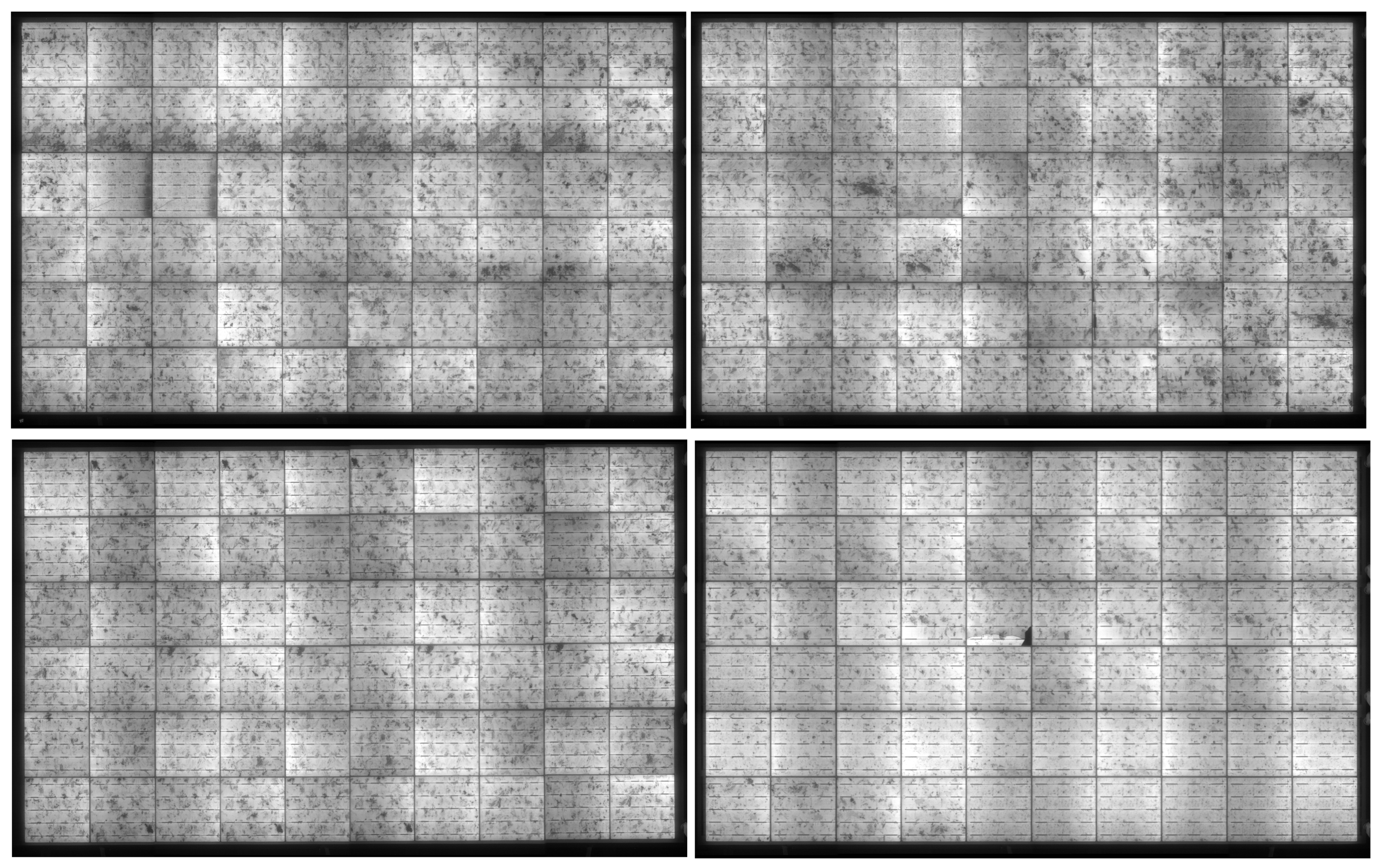
This research study analyzed an extensive dataset comprising 6079 individual solar panel images, encompassing 2245 images of broken panels, 2130 images of clean panels, and 1704 images of dirty panels. Figure 1 offers a visual illustration of the diverse range of panel images employed in this study. The images were methodically categorized into the following three distinctive groups: broken, clean, and dirty. It is noteworthy that test images were not incorporated during the training phase of any algorithm. All images underwent a resizing process to dimensions of 320 by 320 pixels, while the three aforementioned categories (broken, clean, and dirty) were assigned numerical values of 0, 1, and 2, respectively.

To address the class imbalance between the underrepresented broken class and the other classes, data augmentation techniques were applied exclusively to the broken images using a custom Python 3.12 script with the Keras library. Augmentation methods included the following:

• Rotation (±30° range);
• Width/height shift (10% of image size);
• Shear (20% distortion);
• Zoom (20% range);
• Horizontal flipping;
• Nearest-pixel fill mode for boundary regions.

The application of data enrichment was exclusive to the ‘broken’ class, given that the initial number of instances of this class (2245) was not significantly imbalanced in comparison to the other classes (“clean”: 2130, “dirty”: 1704). However, given the presence of complex and rare defects, such as microcracks and delamination, within the ‘broken’ class, a targeted augmentation strategy was employed to facilitate the model’s learning of these variations. The ‘clean’ and ‘dirty’ classes were not augmented due to their adequate representation and reduced variation. The efficacy of these practices is evidenced by the significant enhancement in the performance of the ‘broken’ class observed upon implementing the boosting strategy. Moreover, despite the absence of any boosting applied to the ‘dirty’ and ‘clean’ classes, no statistically significant decline in the accuracy of these classes was observed. This finding further supports the hypothesis that the other classes initially possessed sufficient data and did not require augmentation. The targeted data enrichment strategy applied in this study served to reduce the adverse effects of class imbalance. It resulted in a significant improvement in the model’s performance in the ‘broken’ class.

These techniques generated six augmented variants per original broken image, significantly enhancing the dataset’s diversity and mitigating overfitting risks.

During data splitting for the YOLO-based models, the dataset was partitioned into three subsets:

• 70% training (4254 images);
• 20% validation (1216 images);
• 10% testing (609 images).

Class-specific distributions for YOLO are detailed in Section 3. For the CNN model, a 9-fold cross-validation approach was adopted. The dataset was divided into nine equal folds, with eight folds (≈80%) used for training, one fold (≈10%) for validation, and the final 10% reserved as an independent test set. This ensured no overlap between the training, validation, and testing phases, preserving the integrity of the evaluation.

All images were resized to 320 × 320 pixels to standardize input dimensions, and class labels were encoded numerically (0: broken, 1: clean, and 2: dirty). The dataset and augmentation pipeline were designed to reflect real-world scenarios, ensuring the model’s applicability to practical solar panel inspection tasks.

2.3. Performance Metrics Overview

The proposed model was evaluated in terms of precision, recall, F1-score, accuracy, and ROC (AUC) curve. This study proposes the following formulas for evaluating machine learning performance metrics:

• Precision (Positive Predictive Value): Precision is the ratio of the number of true positive predictions to the total number of positive predictions [44] (defined as Equation (1)).

  $$\mathrm{Precision}={\displaystyle \frac{\mathrm{True} \mathrm{Positives}}{\mathrm{True} \mathrm{Positives}+\mathrm{False} \mathrm{Positives}}}$$

  (1)
• Recall (Sensitivity or True Positive Rate): Recall is the ratio of the prediction of true positives to the total number of actual positives [45] (defined as Equation (2)).

  $$\mathrm{Recall}={\displaystyle \frac{\mathrm{True} \mathrm{Positives}}{\mathrm{True} \mathrm{Positives}+\mathrm{False} \mathrm{Negatives}}}$$

  (2)
• F1-Score: The F1 score is calculated as the harmonic mean of precision and recall, balancing the two (defined as Equation (3) [46]).

  $$\mathrm{F}1\text{-}\mathrm{Score}={\displaystyle \frac{2\times \mathrm{Precision}\times \mathrm{Recall}}{\mathrm{Precision}+\mathrm{Recall}}}$$

  (3)
• Accuracy: The accuracy of a prediction is determined by the ratio of correct predictions to the total number of predictions made [47] (defined as Equation (4)).

  $$\mathrm{Accuracy}={\displaystyle \frac{\mathrm{True} \mathrm{Positives}+\mathrm{True} \mathrm{Negatives}}{\mathrm{Total} \mathrm{Instances}}}$$

  (4)
• Receiver Operating Characteristic (ROC) Curve and Area Under the Curve (AUC): ROC curves graphically represent tradeoffs between sensitivity (true positive rates) and specificity (true negative rates) at different cutoffs. The AUC, which summarizes the performance of the classifier at different cut-offs, is the area under the ROC curve. ROC Curve: The ROC curve plots the true positive rate (sensitivity) against the false positive rate (1—specificity) at various threshold values. The AUC formula is a measure of the area under the ROC curve [44].

In this study, the classification process for the three specified classes—“broken”, “clean”, and “dirty”—was conducted using the structured table provided in Figure 2. This table systematically compares the actual ground truth (actual situation) with the model’s predictions, enabling a detailed classification performance evaluation. Key metrics such as true positive (TP), false negative (FN), and true negative (TN) are explicitly outlined for each class through combinatorial scenarios.

• True Positive (TP): Represents cases where a class is correctly identified. For instance, the “Broken–Broken (TP)” entry denotes cases in which genuinely broken items are accurately classified as broken by the model. Similarly, “Clean–Clean (TP)” and “Dirty–Dirty (TP)” reflect successful predictions for the clean and dirty classes, respectively.
• False Negative (FN): Occurs when instances belonging to a specific class are misclassified into other courses. For the “Broken” class, FN is calculated as the sum of “Broken–Clean” and “Broken–Dirty” cases, indicating broken items incorrectly labeled as clean or dirty. The same logic applies to the FN values for the “Clean” and “Dirty” classes.
• True Negative (TN): Refers to the correct identification of instances not belonging to a target class. For example, the TN value for the “Broken” class aggregates all correctly classified non-broken cases, such as “Clean–Clean”, “Clean–Dirty”, “Dirty–Clean”, and “Dirty–Dirty” combinations.

The table resembles a multi-class confusion matrix, highlighting critical performance metrics (e.g., accuracy, precision, specificity) for evaluating the classifier. Misclassification patterns, such as “Dirty–Broken” or “Clean–Dirty”, reveal where the model struggles, pinpointing areas for refinement. For instance, frequent confusion between “Clean” and “Dirty” may suggest overlapping features or insufficient training data for these classes.

This structured analysis aids in balancing the model’s optimization, ensuring reliable predictions across all classes. This table is a foundational tool for enhancing the classifier’s robustness and generalizability in real-world applications by quantifying errors and successes.

3. Results

The CNN algorithm was evaluated using MATLAB^® R2024a (The MathWorks Inc., Natick, MA, USA) on a system equipped with an Intel^® Core™ i7 CPU (3.6 GHz), 16 GB RAM, and a 64-bit operating system. The computational efficiency of the training and testing processes was further enhanced by leveraging an NVIDIA RTX 4060 GPU, which significantly accelerated model training and inference.

TensorFlow 2.19.0 [48] was employed as the primary framework for implementing deep learning models, providing a flexible and efficient platform for neural network training and optimization. The development and execution of the models were carried out in a Python 3.12 environment, allowing seamless integration of various deep learning libraries and ensuring compatibility with state-of-the-art machine learning tools.

Utilizing these computational resources significantly reduced the training time for each model, enabling faster convergence and improved accuracy. The GPU-accelerated computations were particularly beneficial in handling large image datasets and complex architectures, ensuring that the models effectively learned distinguishing features for solar panel classification. This setup contributed to the overall robustness and efficiency of the proposed methodology, allowing for reliable and scalable implementation in real-world applications.

As previously indicated, CNN’s algorithm has segmented the footage into nine distinct components, constituting 90% of the total. A proportion of the images are used for verification, while the remaining eight are employed for educational purposes. It is important to note that this configuration is subject to dynamic fluctuations with each iteration. Following the conclusion of the son model training, the total number of models has been increased to ten. The duration of the training for the model was approximately five hours. Consequently, the total development time for the model was 50 h, according to the CNN algorithm.

The temporal parameters of YOLO algorithms are contingent upon the assigned weight. The YOLO model is available in five different weights. For instance, the YOLOv8 model is available in five sizes: nano, small, medium, large, and large. YOLOv9 is distinguished by its capacity to adapt to various dimensions, encompassing tiny, small, medium, compact, and extended sizes. The duration is increased in proportion to the extent to which the model is expanded. The training process for each iteration of the YOLO model has been meticulously documented. It has been determined that the time required to complete the smallest model is approximately one hour, while the time required to complete the larger model, designated ‘larger’, is approximately three hours. The completion of the larger loads, designated ‘Orta’, was achieved within a time frame of approximately nine hours. The training program was completed in approximately 16 h for the larger and more compact weights, and the training for the largest weights was concluded within 24 h.

The utilization of the YOLOv8 and YOLOv9 algorithms is imperative. The following versions are employed: PyCharm (2024.2.2), Python (3.12), certifi = (2024.8.30), charset-normalizer = (3.3.2), colorama = (0.4.6), contourpy = (1.3.0), cycler = (0.12.1), filelock = (3.16.1), fonttools = (4.54.0), fsspec = (2024.9.0), idna = (3.10), importlib_resources = (6.4.5), Jinja2 = (3.1.4), kiwisolver = (1.4.7), MarkupSafe = (2.1.5), matplotlib = (3.9.2), mpmath = (1.3.0), networkx = (3.2.1), numpy = (1.26.4), opencv-python = (4.10.0.84), packaging = (24.1), pandas = (2.2.3), pillow = (10.4.0), psutil = (6.0.0), py-cpuinfo = (9.0.0), pyparsing = (3.1.4), python-dateutil = (2.9.0.post0), pytz = (2024.2), PyYAML = (6.0.2), requests = (2.32.3), scipy = (1.13.1), seaborn = (0.13.2), six = (1.16.0), sympy = (1.13.3), torch = 2.4.1, torchaudio = (2.4.1), torchvision = (0.19.1), tqdm = (4.66.5), typing_extensions = (4.12.2), tzdata = (2024.2), ultralytics = (8.2.100), ultralytics-thop = (2.0.8), urllib3 = (2.2.3), and zipp = (3.20.2).

3.1. Dataset Augmentation

This study employed a unique and proprietary dataset consisting of images of clean, dirty, and broken solar panels. However, a significant imbalance was observed in the dataset, as the number of images depicting broken panels was relatively lower compared to the clean and dirty panel images. A data augmentation pipeline was developed using Python 3.12 and the Keras library to address this issue and mitigate the risk of overfitting. This augmentation process aimed to enhance the representation of broken panel images while improving the overall generalization capability of the deep learning models.

The effectiveness of data augmentation techniques depends on the diversity of the dataset, which should ideally include images captured under various real-world conditions. In this study, augmentation was performed by incorporating images taken at different distances, from various angles, under varying lighting conditions, and with different camera movements (e.g., panning and tilting). This approach transformed a single original image into six distinct variations, enriching the dataset and providing the model with a broader range of training examples.

The augmentation techniques applied in this study are as follows:

• Rotation Augmentation: To improve model robustness by exposing it to different orientations, the images were rotated from 0° to 30°. The degree of rotation was carefully limited to prevent the loss of critical features related to broken panels.
• Width and Height Shift Augmentation: To simulate slight displacements in real-world images, the original images were shifted horizontally and vertically by 10% of their size. This technique helps the model recognize solar panel defects even when positioned at different locations in the frame.
• Shear Augmentation: Image distortion was introduced by tilting the images with a shear intensity of 0.2. This transformation ensured that key structural features remained identifiable while improving the model’s ability to detect deformations and cracks in solar panels.
• Zoom Augmentation: Images were either enlarged or shrunk within a zoom range of 0.2, effectively creating variations that simulate differences in camera distance and focal length.
• Flip Augmentation: Images were flipped along the horizontal axis, allowing the model to recognize panel conditions from different perspectives. Vertical flipping was avoided to maintain the realistic orientation of the solar panels.
• Fill Mode: At the end of the augmentation process, fill mode was applied to ensure newly generated pixels were assigned values from their nearest neighboring pixels, preventing artifacts and inconsistencies in the transformed images.

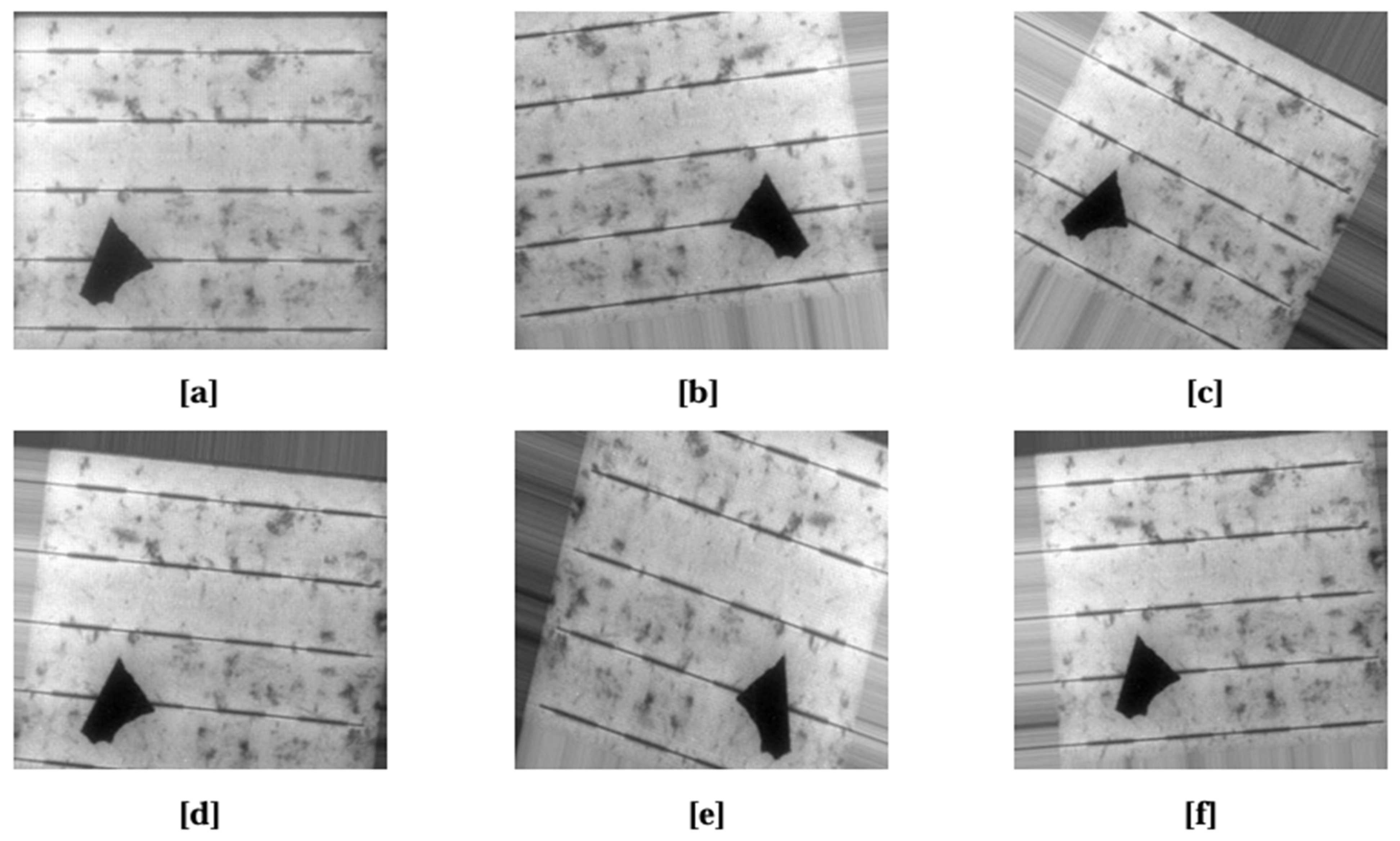
This augmentation strategy significantly improved the diversity and robustness of the dataset, allowing the deep learning models to generalize more effectively to unseen images. A sample visualization of the data augmentation outcomes is provided in Figure 3, illustrating the variations generated from an input image.

3.2. Dataset Preparation

In this study, a total of 6079 single solar panel images were utilized, categorized into three distinct classes: broken, clean, and dirty. Specifically, the dataset comprised 2245 images of broken panels, 2130 images of clean panels, and 1704 images of dirty panels. Each class was assigned a numerical label for model training purposes, where broken panels were labeled as 0, clean panels as 1, and dirty panels as 2.

To ensure consistency in model training and evaluation, all images were resized to 320 × 320 pixels, preserving their aspect ratios and essential structural features. The dataset was carefully partitioned to prevent data leakage, ensuring that test images were not included in the training phase of any model.

For the YOLO-based models (YOLOv8-m and YOLOv9-e), the dataset was divided into the following three subsets:

• 70% of the images were allocated for training;
• 20% were designated for validation;
• 10% were reserved for testing.

The YOLO algorithm is predicated on the principle of data segmentation, with the primary rationale for this being the enhancement of the precision of the model’s performance evaluation during the training process. The dataset is thus divided into three segments: 70% for training, 20% for validation, and 10% for testing. The prevailing convention is to allocate 80% of the resources to training, 10% to validation, and 10% to testing to facilitate the model’s capacity to learn from a more extensive array of samples, as characterized by a greater proportion of training data. However, in this study, the proportion of the validation set is increased to 20% to detect the overfitting tendencies of the model earlier and more effectively during training. Consequently, it is feasible to calibrate the model parameters and hyperparameters through the evaluation process on the validation set. The fundamental rationale behind the 70–20–10% data separation is to enhance the efficacy of monitoring training performance and augment the model’s generalization capability.

This split ensured that the models were trained on a diverse set of images while maintaining an independent test set for unbiased performance evaluation. The exact number of images assigned to each subset is provided in

Table 1. Number of images based on classes and usages for YOLO.

	Train	Validation	Test
Broken	1192	341	171
Clean	1491	426	213
Dirty	1571	449	225

.

In contrast, for the CNN model, the dataset was first classified according to the three predefined categories: broken, clean, and dirty. The CNN algorithm itself handled the automated partitioning of images into training, validation, and testing subsets, ensuring an optimal distribution for model training.

This structured approach to dataset preparation was essential for maintaining model generalizability and ensuring fair comparisons between different deep learning architectures.

3.3. YOLOv8

The YOLOv8 object detection model represents a significant advancement on previous iterations of the YOLO series, characterized by integrating a more efficient and scalable architecture. The network consists of three primary components: the backbone, the neck, and the head. The backbone is typically based on CSPDarknet and is responsible for extracting hierarchical features by utilizing multiple convolutional layers, accompanied by batch normalization and leaky ReLU activations. The subsequent neck element (which incorporates PANet and SPPF [Spatial Pyramid Pooling—Fast]) enhances feature fusion and spatial information. Finally, the head performs object classification and bounding box regression using anchor-free mechanisms, thus improving detection accuracy. YOLOv8 adopts dynamic anchor assignments and decoupled heads, refining detection precision while reducing computational complexity. The efficacy of these modifications is evidenced by the capacity of YOLOv8 to attain superior speed and accuracy, rendering it particularly well-suited for real-time applications such as solar panel defect detection.

In the YOLOv8 framework, five distinct model weight configurations are available, namely nano, small, medium, large, and X-large, each representing progressively increasing model complexities. Specifically, the nano model corresponds to the smallest architecture, followed by the small model, which offers a balance between computational efficiency and accuracy. The medium model serves as an intermediate option, while the large and X-large models provide enhanced feature extraction capabilities with increased parameter complexity.

To ensure a comprehensive evaluation of model performance, all five weight configurations were utilized during both the training and testing phases. Regardless of the model size, the training process was conducted for a total of 100 epochs, ensuring sufficient iterations for learning optimization while maintaining consistency across different weight configurations.

The statistical data presented in

Table 2. Training parameters for YOLOv8 based on model weights.

Model	Score of Class	Precision–Recall	F1-Score	Precision	Recall
Nano	class score 0	0.992	-	-	-
	class score 1	0.965	-	-	-
	class score 2	0.947	-	-	-
	all classes	0.968 mAP@0.5	0.91 at 0.489	1.00 at 1.000	1.00 at 1.000
Small	class score 0	0.993	-	-	-
	class score 1	0.965	-	-	-
	class score 2	0.956	-	-	-
	all classes	0.971 mAP@0.5	0.93 at 0.447	1.00 at 1.000	1.00 at 1.000
Medium	class score 0	0.993	-	-	-
	class score 1	0.967	-	-	-
	class score 2	0.952	-	-	-
	all classes	0.971 mAP@0.5	0.93 at 0.401	1.00 at 1.000	1.00 at 1.000
Large	class score 0	0.993	-	-	-
	class score 1	0.967	-	-	-
	class score 2	0.952	-	-	-
	all classes	0.971 mAP@0.5	0.93 at 0.401	1.00 at 1.000	1.00 at 1.000
X-large	class score 0	0.992	-	-	-
	class score 1	0.965	-	-	-
	class score 2	0.947	-	-	-
	all classes	0.971 mAP@0.5	0.93 at 0.401	1.00 at 1.000	1.00 at 1.000

demonstrate that among the various model weight configurations utilized in YOLOv8, the small and medium models outperform the others regarding precision–recall and F1-score. These findings suggest that these two models better balance computational efficiency and classification performance, making them more suitable for solar panel defect detection.

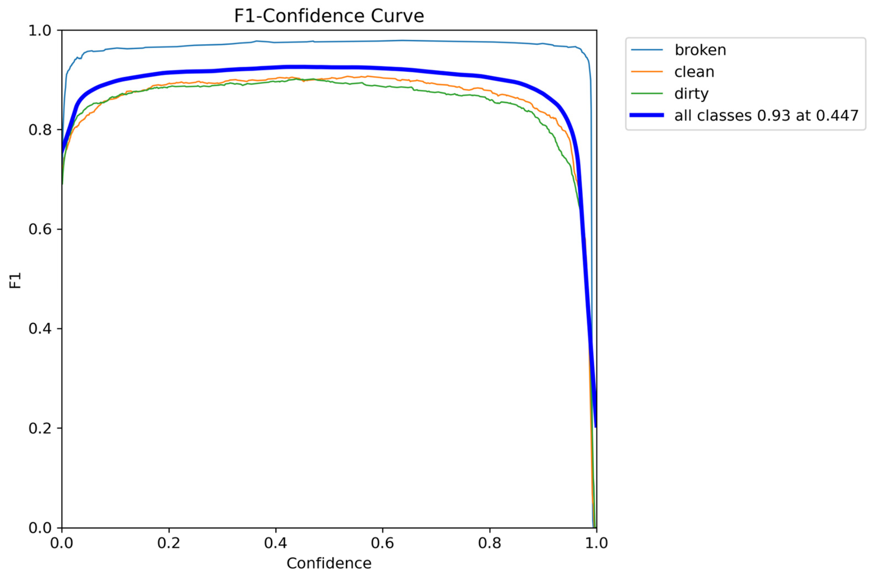
Furthermore, the graphical analysis in Figure 4 reveals that the F1-score curve reaches its highest value of 0.93 at a specific threshold of 0.447 for the small model. These observations indicate that the medium model exhibits a lower decision threshold than the small model, which classifies instances with higher confidence at an earlier stage. However, despite this difference in threshold values, both models’ overall F1 confidence scores remain identical, highlighting their comparable effectiveness in classification tasks.

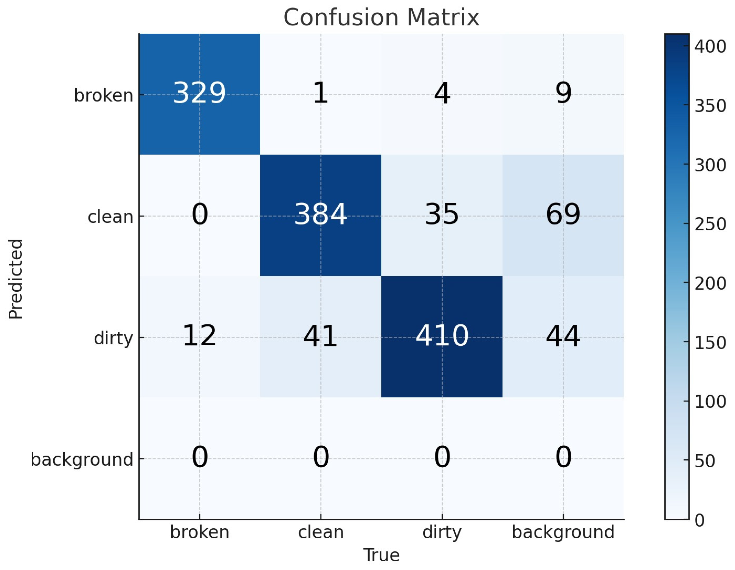
The confusion matrices for the YOLOv8-s and YOLOv8-m models are provided in Figure 5 and Figure 6, offering a comprehensive visualization of their classification performance. In these matrices, the false negative (FN) values are represented within the background row, whereas the false positive (FP) values are positioned in the background column. The true positive (TP) values indicate correctly classified instances and are located along the diagonal axis extending from the top-left to the bottom-right of the matrix. The true negative (TN) values are also derived based on Figure 2.

For the YOLOv8-s model, the performance metrics computed from the confusion matrix indicate that the sensitivity (recall) is 1.00, meaning the model successfully detects all relevant instances without missing any positive cases. The specificity, which measures the model’s ability to identify negative cases correctly, is 0.9504, reflecting its effectiveness in minimizing false positives. Lastly, the overall accuracy of the YOLOv8-s model is calculated as 0.9659, demonstrating its high reliability in distinguishing between the three solar panel conditions.

Similarly, for the YOLOv8-m model, the corresponding values derived from its confusion matrix indicate that the sensitivity remains at 1.00, confirming that this model, like YOLOv8-s, does not miss any positive instances. However, the specificity of YOLOv8-m is slightly higher at 0.9594, suggesting a marginal improvement in correctly identifying negative cases. Additionally, the accuracy of the YOLOv8-m model is recorded as 0.9726, showing that it slightly outperforms the YOLOv8-s model in overall classification performance. These findings highlight that while both models demonstrate strong predictive capabilities, the YOLOv8-m model exhibits a slight edge in specificity and overall accuracy.

The results pertaining to the accuracy, specificity, and sensitivity of YOLOv8-s and YOLOv8-m are displayed in

Table 3. Accuracy, specificity, and sensitivity results for YOLOv8-s and YOLOv8-m based on confusion matrix.

	Accuracy	Sensitivity	Specificity
YOLOv8-s	96.59%	100%	95.04%
YOLOv8-m	97.26%	100%	95.94%

. In addition, Figure 5 and Figure 6 show the confusion matrix of YOLOv8-s and YOLOv8-m respectively.

Although the sensitivity values of both the small and medium YOLOv8 models are comparable, the medium model demonstrates slightly higher accuracy and specificity scores. This indicates that while both models effectively identify positive instances, the medium model is marginally better at correctly classifying negative cases, improving overall performance.

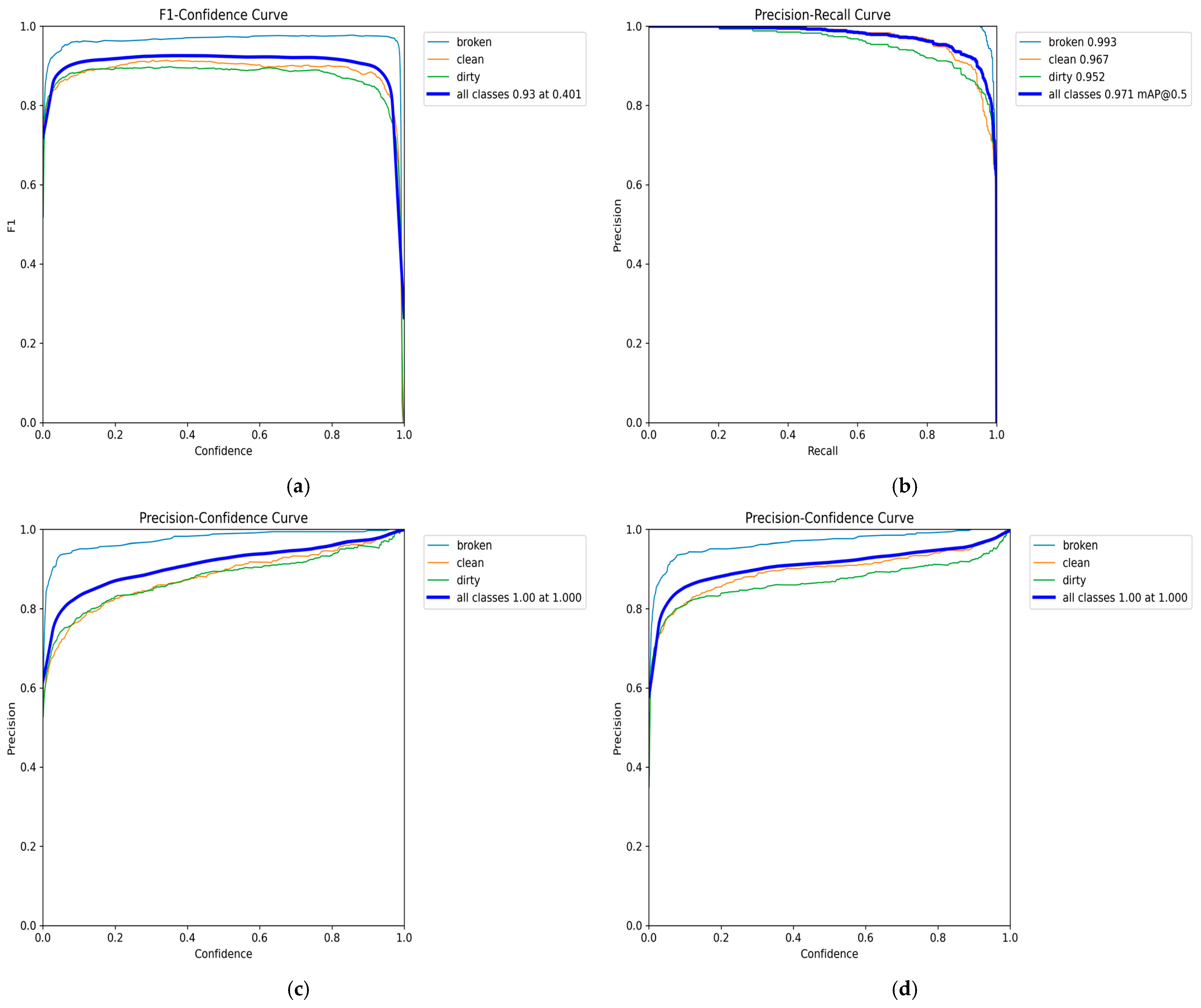
A more detailed analysis of the precision–recall values across different image categories provides further insights into their comparative performance. Specifically, for the dirty panel class, as depicted in Figure 7, the small model achieves a precision–recall value of 0.956. In contrast, in Figure 8b, the medium model attains a slightly lower precision–recall score of 0.952. This suggests that the small model is marginally more effective for identifying dirty panels than the medium model.

Conversely, when analyzing the clean panel class, the precision–recall score of the medium model surpasses that of the small model. As shown in Figure 7 and Figure 8b, the medium model achieves a precision–recall value of 0.967, while the small model records a slightly lower value of 0.965. Although this difference is minimal, the medium model performs slightly better at detecting clean panels.

Finally, when considering the broken panel class and the overall classification performance across all categories, both models exhibit identical precision–recall values, reinforcing that their ability to detect broken panels remains consistent. These results suggest that while the small model excels in detecting dirty panels, the medium model shows a slight advantage in identifying clean panels and offers improved specificity and accuracy overall.

As illustrated in Figure 8a, the F1-score curve for the medium model attains its peak value of 0.93 at a slightly lower threshold of 0.401.

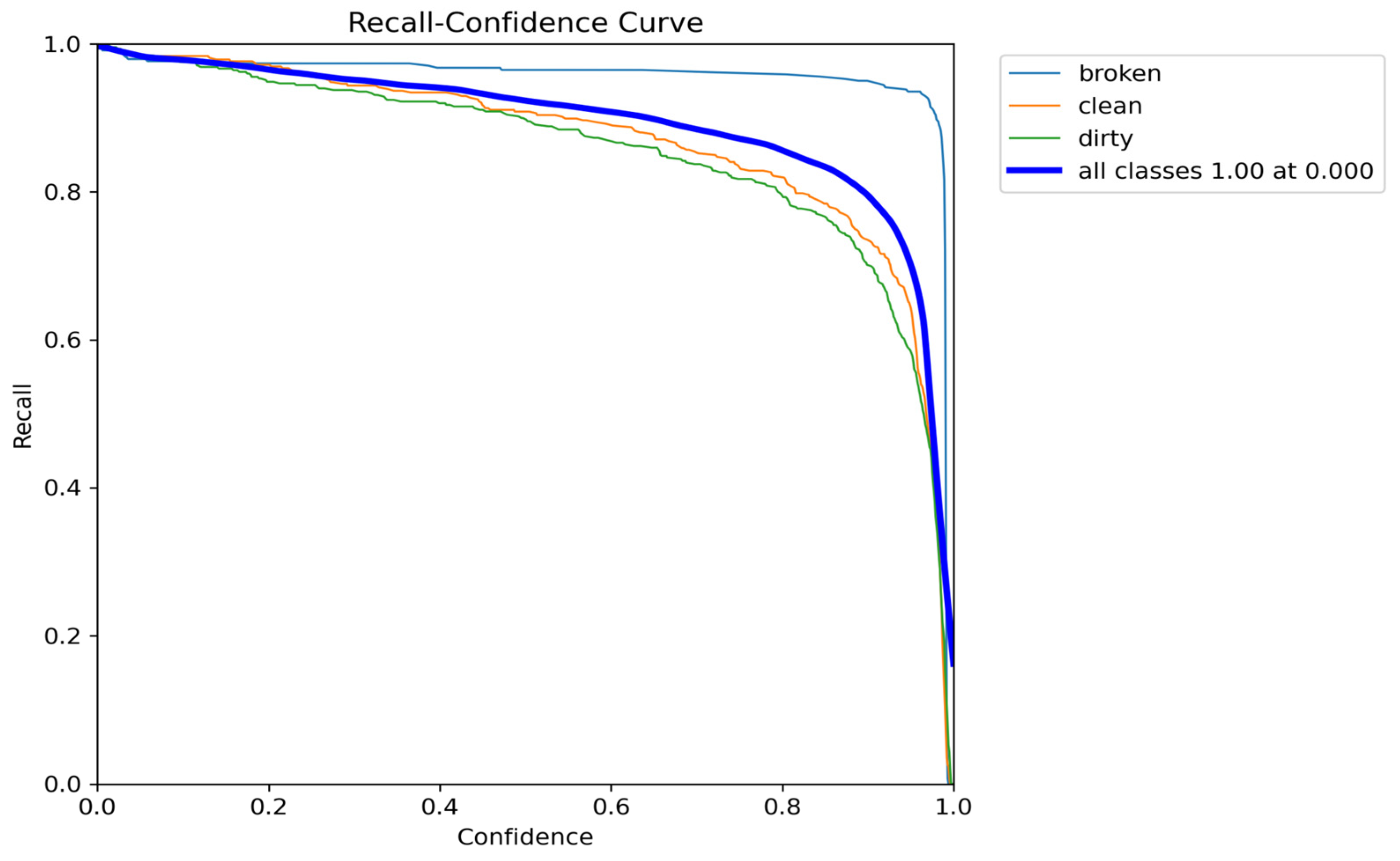
As illustrated in Figure 9 and Figure 10, the recall value reaches 1.00, indicating that the model successfully identifies all relevant instances. This suggests that no positive cases were misclassified, demonstrating the model’s high sensitivity.

Figure 11 and Figure 12 provide a comprehensive summary of the comparative performance of the YOLOv8-s and YOLOv8-m models throughout the training process, offering valuable insights into their respective behaviors regarding loss reduction, precision, recall, and validation stability.

Based on the observed results, selecting the small model as the optimal choice in YOLOv8 is justified for several reasons. One of the key findings is that, when analyzing Figure 11, which represents the training performance metrics, it becomes evident that the loss values decrease at a slightly more consistent rate in the small model compared to the medium model. This indicates that the small model exhibits a more stable convergence pattern, which is crucial in ensuring efficient learning and reducing overfitting risks.

Additionally, an evaluation of precision and recall values across training iterations reveals that the small model maintains higher stability than the medium model. The fluctuations in these metrics are more pronounced in the medium model, whereas in the small model, they remain relatively steady, contributing to improved reliability during inference.

A similar trend is observed when analyzing Figure 12, representing validation performance metrics. The mean average precision (mAP) values for the small model demonstrate a more stable pattern than the medium model, further reinforcing its robustness [49,50]. This suggests that the small model generalizes well across different validation sets, ensuring its predictions remain reliable when exposed to unseen data.

While minor oscillations in performance metrics are present in both models, they are not critical and can be attributed to the weight variations during the training process. The results collectively suggest that the YOLOv8-s model, despite being a minor architecture, offers more excellent stability, a more consistent loss reduction, and improved generalization compared to the YOLOv8-m model, making it a strong candidate for optimal model selection in this study.

A comparative analysis of the YOLOv8-s and YOLOv8-m models reveals that they demonstrate similar F1 scores, precision values, recall values, and precision–recall metrics, indicating comparable classification performance. However, despite these similarities, the YOLOv8-m model exhibits slightly higher accuracy and specificity values than the YOLOv8-s model, making it marginally more effective in distinguishing between different classes.

The only aspect in which the YOLOv8-s model demonstrates superior performance is its loss graphs’ stability throughout the training process, suggesting a more consistent learning pattern. Nevertheless, considering the overall classification metrics, the YOLOv8-m model outperforms YOLOv8-s, offering slightly improved parameters and thus proving to be the most effective among the YOLOv8 models in this study.

3.4. YOLOv9

YOLOv9 is an advanced object detection model that builds upon the strengths of its predecessor, YOLOv8, while introducing key optimizations for enhanced accuracy and robustness. The model utilizes a more efficient backbone, often integrating features from Scaled-YOLOv4 and transformer-based architectures to improve feature extraction. The neck incorporates an upgraded FPN+PAN structure, enabling better multi-scale feature fusion for effectively detecting small and large objects. A notable distinction of YOLOv9 is its incorporation of an adaptive spatial feature selection mechanism, a feature absent in YOLOv8. This mechanism serves to reduce redundant computations, thereby enhancing detection reliability. Furthermore, the model has been endowed with advanced anchor-free strategies and gradient-guided optimizations, contributing to object classification and localization refinement. The aforementioned enhancements collectively render YOLOv9 particularly effective in scenarios requiring high precision, such as detecting defects in solar panels under varying environmental conditions.

In the YOLOv9 framework, five distinct model weight configurations are utilized, namely tiny, small, medium, compact, and extended, representing progressively increasing model complexities. The tiny model corresponds to the most miniature architecture, followed by the small model, which balances computational efficiency and accuracy. The medium model is an intermediate option, while the compact and extended models provide enhanced feature extraction capabilities with increasing parameter complexity.

All five weight configurations were employed during the training and testing phases to ensure a comprehensive evaluation of model performance. Regardless of the model size, the training process was conducted for 100 epochs, ensuring sufficient iterations for optimizing the learning process while maintaining consistency across different weight configurations.

Transfer learning was not employed in training the YOLO model; instead, the model was trained from scratch. The model parameters are initialized with random weights during training to learn unique features specific to the data. It has been demonstrated that training from scratch is advantageous in two particular cases. Firstly, in the event of the target dataset containing features significantly different from those of the pre-trained datasets. Secondly, if the training dataset is sufficiently comprehensive in size, in this case, since extraneous and irrelevant features do not constrain the model’s parameters, it develops a more optimal representation capability specific to the target dataset. Consequently, the model demonstrates superior data-specific performance without being influenced by the potential bias introduced by general pre-training. Given the considerable magnitude of the dataset, the optimal approach would be to initiate training from the outset instead of employing the transfer learning strategy.

YOLOv8 and YOLOv9 parameters are as follows: epochs: 100, batch: 16, imgsz: 320, device: auto, workers: 8, optimizer: SGD, lr0: 0.01, lrf: 0.01, momentum: 0.937, weight_decay: 0.0005, warmup_epochs: 3.0, warmup_momentum: 0.8, warmup_bias_lr: 0.1, box: 7.5, cls: 0.5, dfl: 1.5, hsv_h: 0.015, hsv_s: 0.7, hsv_v: 0.4, degrees: 0.0, translate: 0.1, scale: 0.5, flipud: 0.0, fliplr: 0.5, mosaic: 1.0, mixup: 0.0, and copy_paste: 0.0.

The data presented in

Table 4. Training parameters for YOLOv9 based on model weights.

Model	Score of Class	Precision–Recall	F1-Score	Precision	Recall
Tiny	class score 0	0.992	-	-	-
	class score 1	0.964	-	-	-
	class score 2	0.940	-	-	-
	all classes	0.965 mAP@0.5	0.91 at 0.449	1.00 at 1.000	1.00 at 1.000
Small	class score 0	0.992	-	-	-
	class score 1	0.967	-	-	-
	class score 2	0.943	-	-	-
	all classes	0.967 mAP@0.5	0.92 at 0.564	1.00 at 1.000	1.00 at 1.000
Medium	class score 0	0.992	-	-	-
	class score 1	0.965	-	-	-
	class score 2	0.946	-	-	-
	all classes	0.967 mAP@0.5	0.92 at 0.528	1.00 at 1.000	1.00 at 1.000
Compact	class score 0	0.993	-	-	-
	class score 1	0.966	-	-	-
	class score 2	0.945	-	-	-
	all classes	0.968 mAP@0.5	0.91 at 0.401	1.00 at 1.000	1.00 at 1.000
Extended	class score 0	0.993	-	-	-
	class score 1	0.965	-	-	-
	class score 2	0.946	-	-	-
	all classes	0.968 mAP@0.5	0.92 at 0.435	1.00 at 1.000	1.00 at 1.000

indicate that the extended model weight achieves the highest precision–recall and F1-score compared to the other model weights, demonstrating superior overall performance.

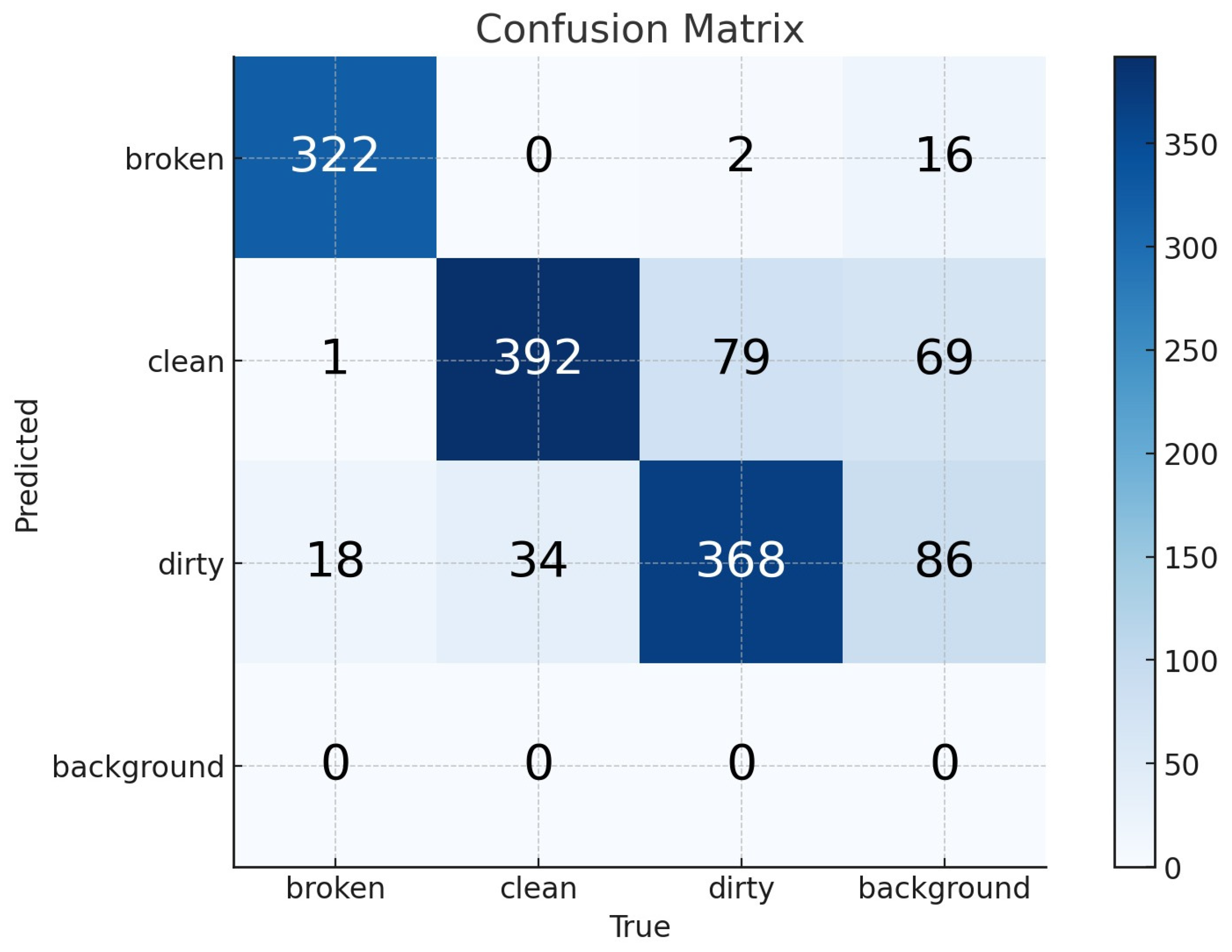
As shown in Figure 13, the F1-score curve reaches its maximum value of 0.92 at a specific threshold of 0.435, highlighting the optimal balance between precision and recall for this model configuration. In addition, Figure 14 show the confusion matrix of YOLOv8-e.

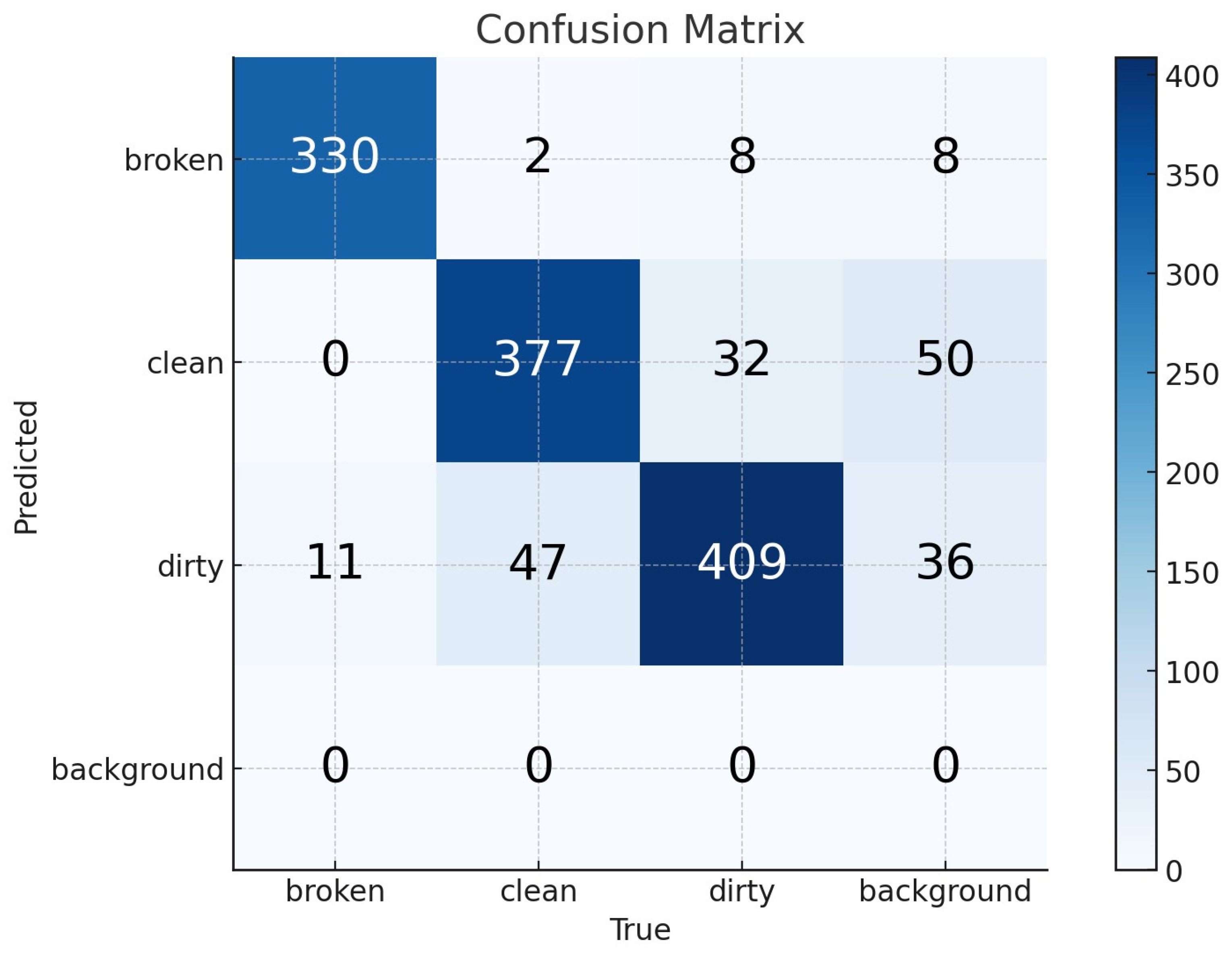
In the YOLOv9-s model, the sensitivity, specificity, and accuracy values derived from the confusion matrix are 1.00, 0.9307, and 0.9518, respectively.

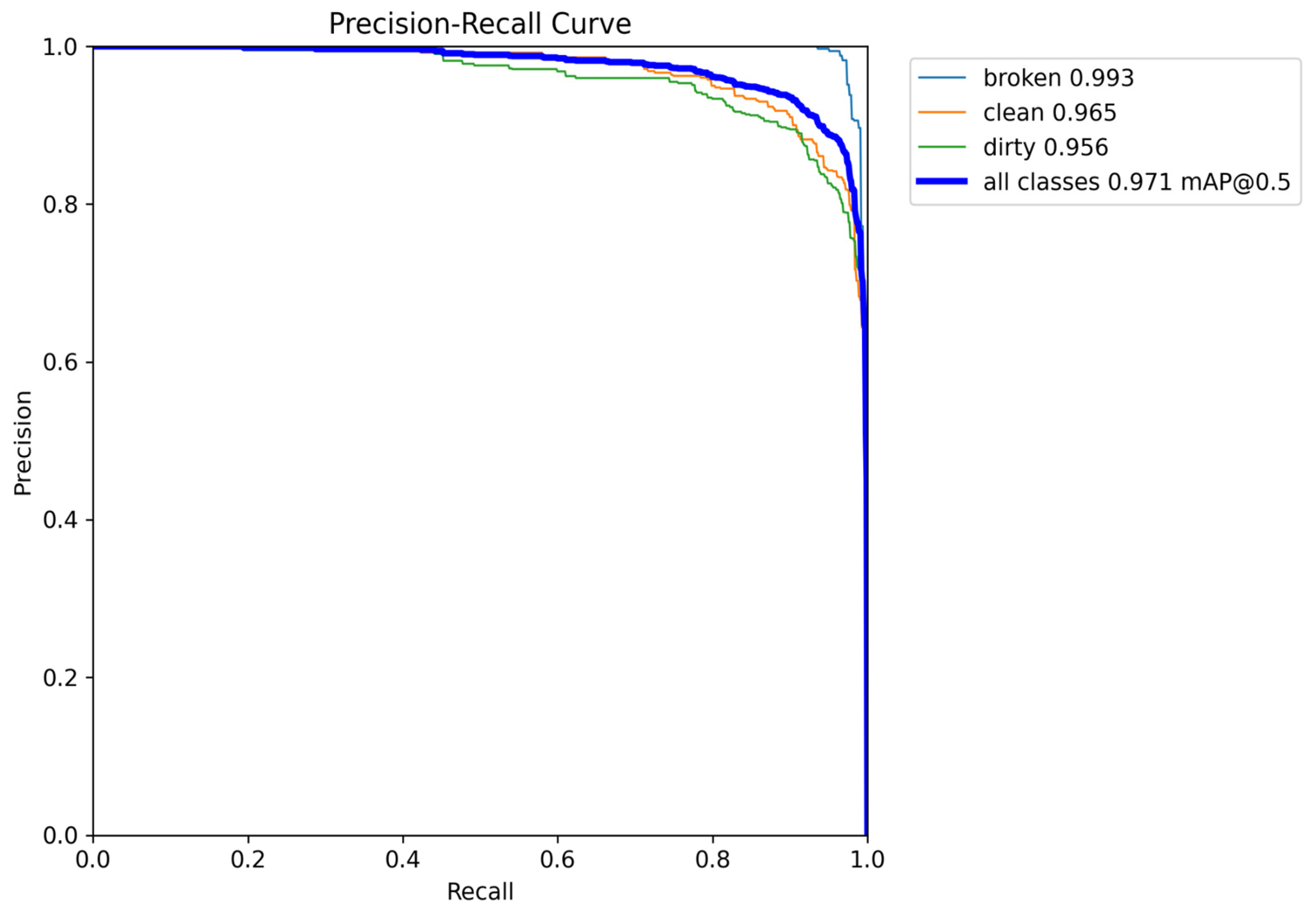
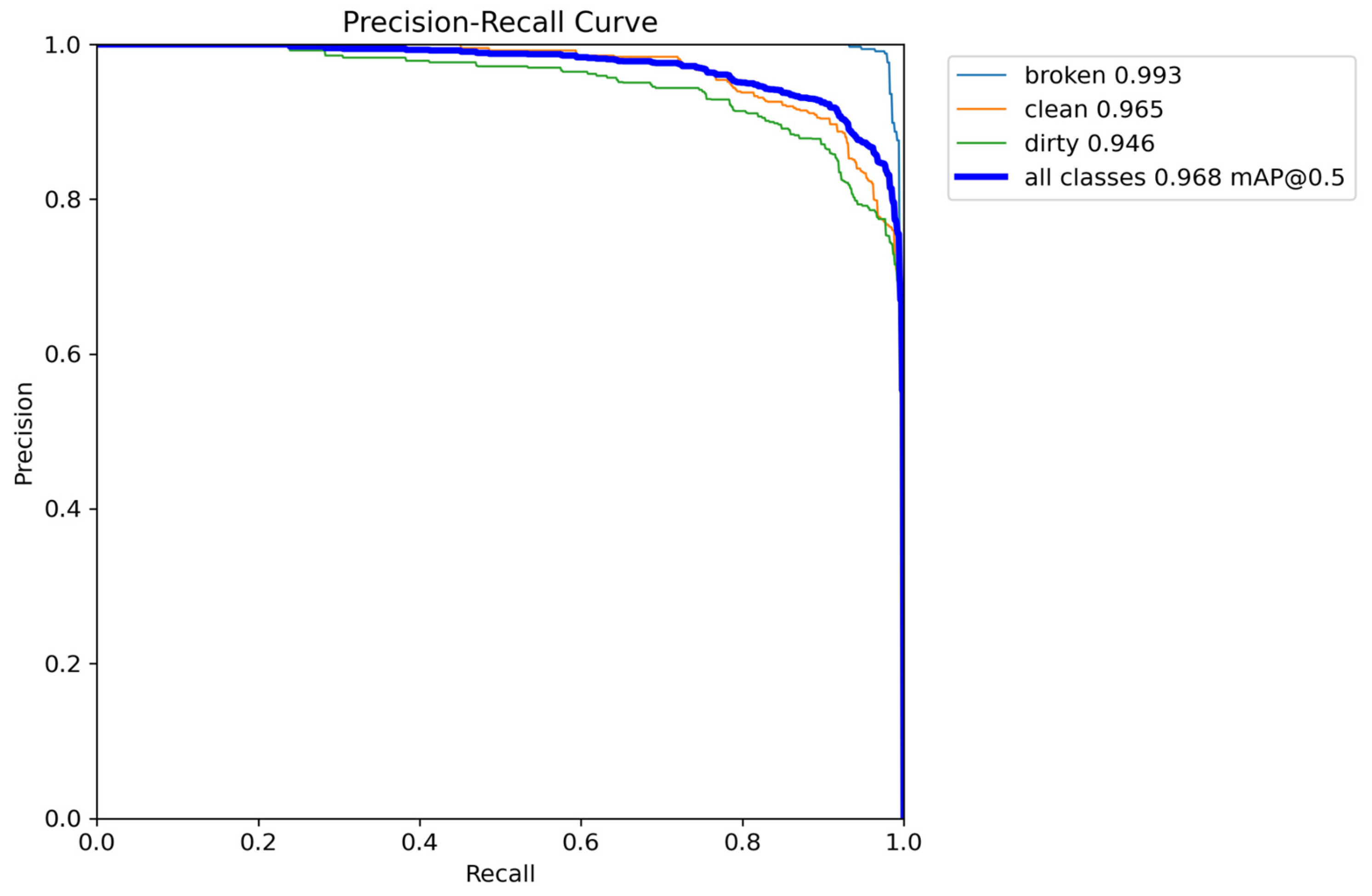
Figure 15 provides a detailed visualization of the precision–recall curve values for each image category, demonstrating the model’s effectiveness in classifying solar panels. The broken panel class achieves the highest precision–recall value of 0.993, followed by the clean panel class with 0.965 and the dirty panel class with 0.946, indicating substantial classification accuracy across all categories. Furthermore, the overall mean average precision (mAP@0.5) across all classes is 0.968, highlighting the model’s robustness.

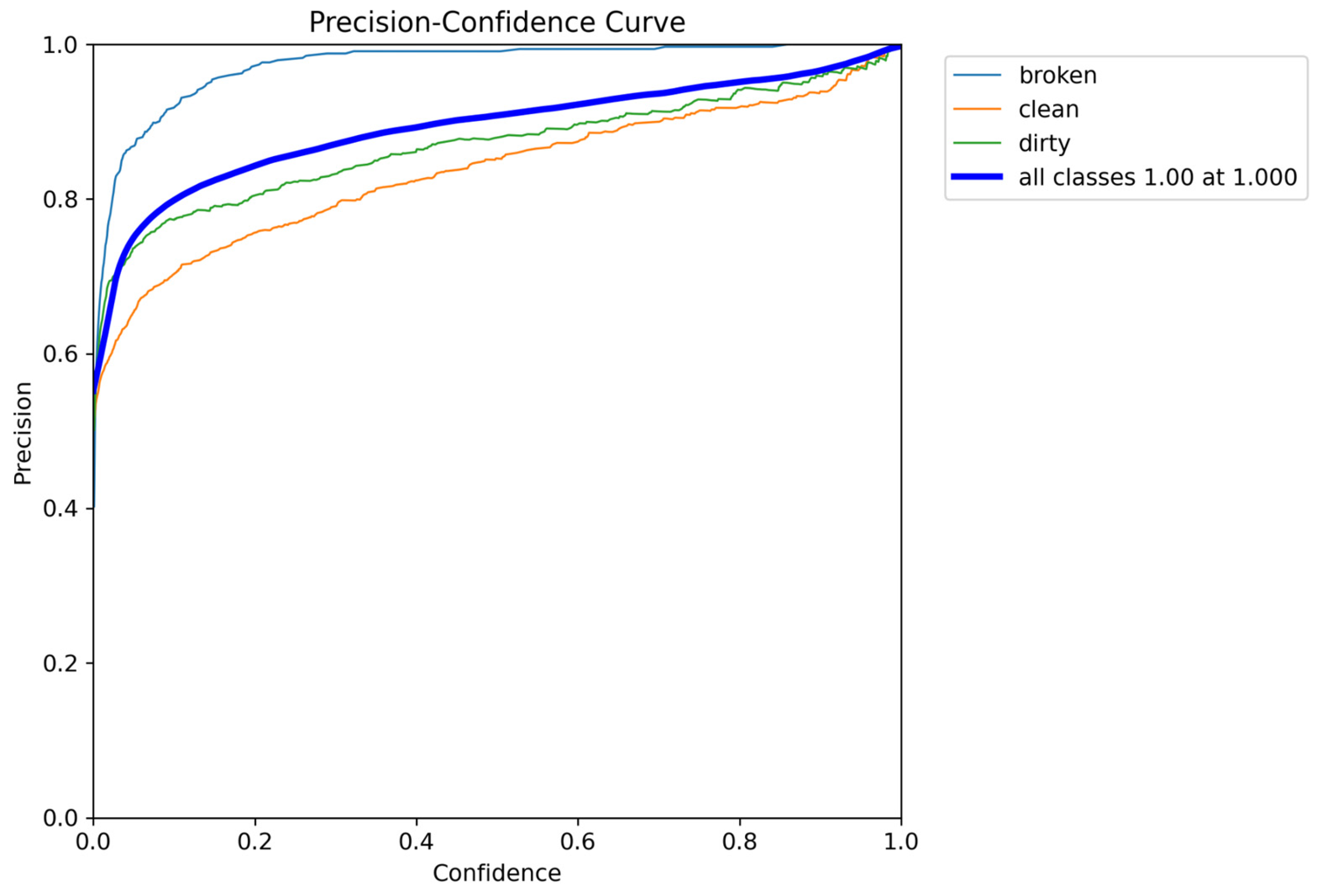
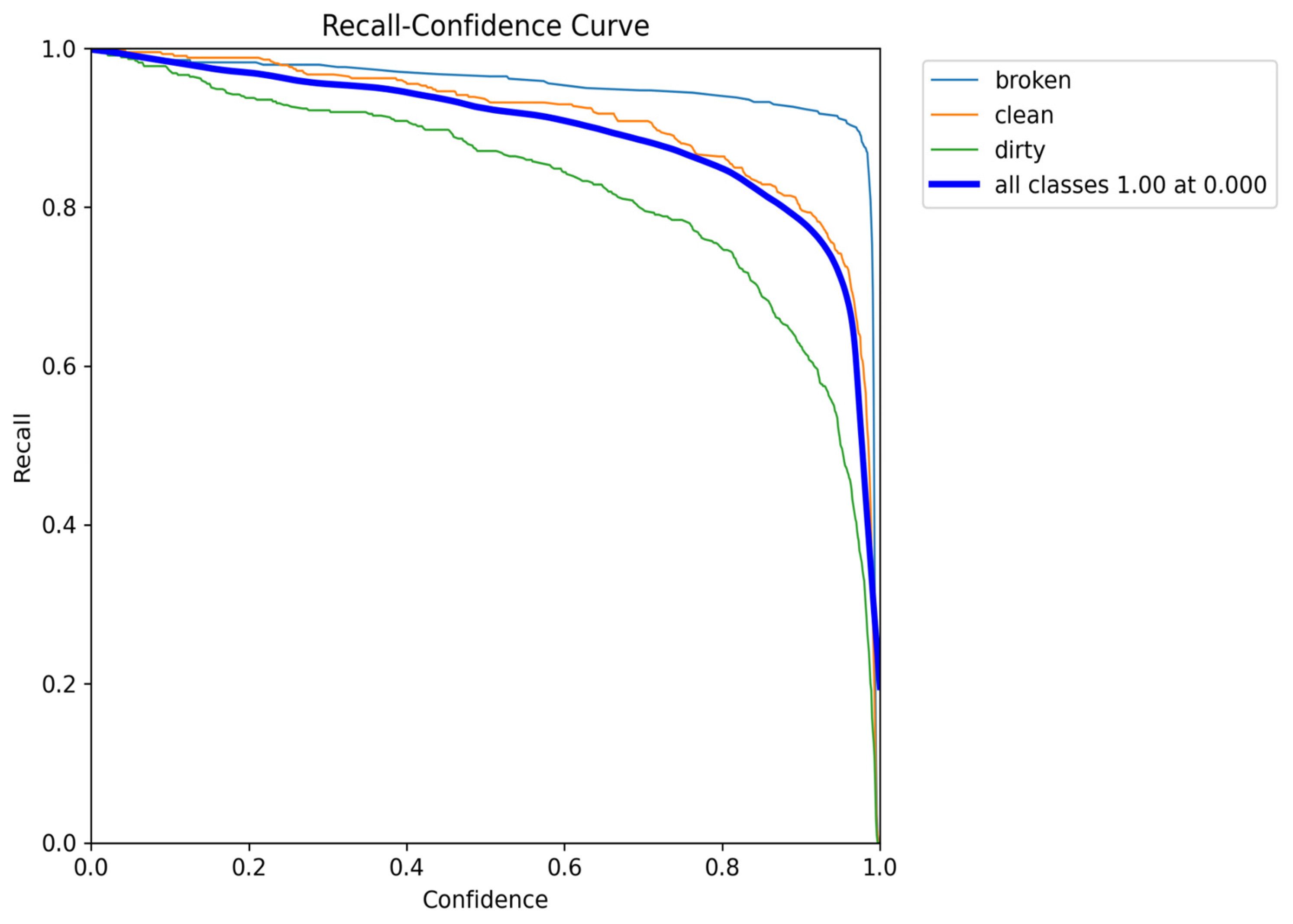
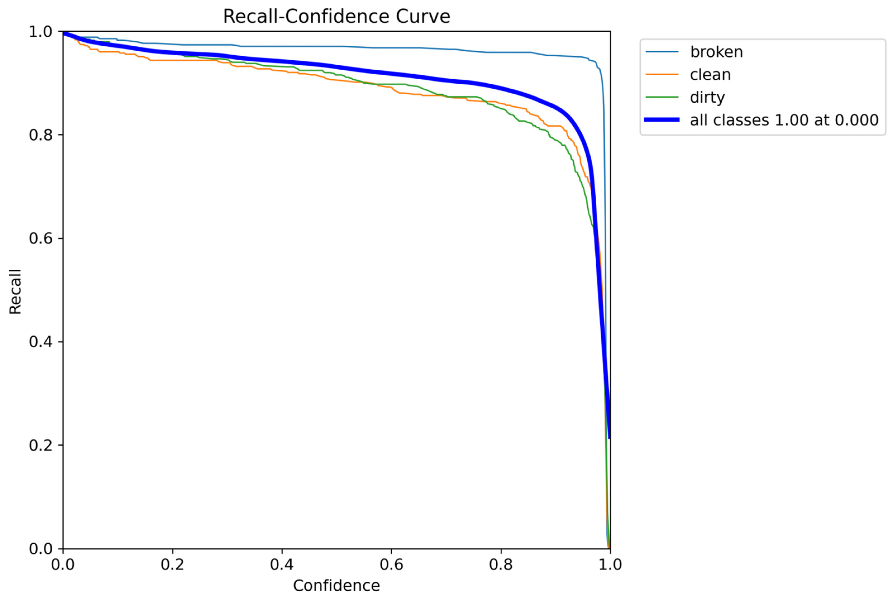
As illustrated in Figure 16, the precision value reaches 1.00, reinforcing the model’s ability to make highly confident positive predictions with minimal false positives. In addition, Figure 17 shows the recall–confidence curve for YOLOv9-e.

Figure 18 illustrates a consistent decline in box loss values, indicating that the model effectively minimizes errors in object localization as training progresses. Simultaneously, precision and recall values gradually increase, reflecting improvements in the model’s ability to identify and classify solar panel conditions correctly. The trends observed in these graphs confirm that the training process was executed correctly, leading to a well-optimized and stable model with enhanced detection capabilities.

3.5. CNN

In the CNN model, the training process was initiated by first separating the test images from the training dataset to ensure an unbiased evaluation. The remaining images were then divided into nine equal parts for training and validation using the k-fold cross-validation approach. In this method, eight parts, representing 80% of the dataset, were used for training in each iteration, while the remaining one part, accounting for 10% of the dataset, was designated for validation. The final 10% of images were set aside for independent testing. This structured division was strictly followed to prevent data leakage, ensuring that the test images were not used during training and preserving the integrity of the evaluation process.

The CNN architecture under consideration consists of 21 layers in total. The sequence of layers is as follows: firstly, an ImageInputLayer is used as the input layer, followed by five Convolution2dLayers, five ReLULayers, and five MaxPooling2dLayers. Subsequently, two fully connected layers, one ReLU layer, one softmax layer, and one classification layer are employed. The function of the latter is to facilitate classification.

Each convolution layer comprises 128 filters, with the filter size set at 5 × 5. The rectified linear unit (ReLU) was employed as the activation function following each convolution layer. The pooling process was performed as maximum pooling (max pooling) with a size of 2 × 2 after each convolution and ReLU block.

The fully connected layers (fullyConnectedLayer) comprise 256 and 3 neurons, respectively. The softmax layer obtains the probabilities in the output layer, and the final layer performs classification.

In addition, the internal functions of MATLAB (namely, train network and classify) were utilized during the training and evaluation phases, with the models being trained on a GPU. Stochastic gradient descent (SGDM) optimization and cross-validation (k-fold cross-validation, K = 9) were preferred in the training process.

The total number of layers was determined by considering all components in the deep learning model utilized. The model begins with an image input layer ([320 320 3]), which processes the input images. For feature extraction, the architecture includes five convolutional layers (Convolution2dLayer), five ReLU activation layers (ReLULayer), and five max-pooling layers (MaxPooling2dLayer). The fully connected and output layers consist of one fully connected layer (256), one ReLU activation, and one fully connected layer (3), followed by a softmax and a classification layer. Summing these components, the model consists of 21 layers in total.

From a neuron activation perspective, the fully connected layers play a decisive role. The fullyConnectedLayer (256) consists of 256 neurons, while the fullyConnectedLayer (3) has three neurons. Although ReLU layers are activated after convolutional and fully connected layers, they do not directly contribute to the total neuron count. Based on this structure, the model’s total number of active neurons is calculated as 259.

In terms of architectural design, the CNN model was configured with the following parameters:

• Padding: 1;
• Stride: 2;
• Filter Size: 5 × 5;
• Number of Filters: 128;
• Total Layers: 5.

Each layer was designed with optimized stride, padding, and activation functions to ensure effective feature extraction and classification. The training parameters were configured as follows:

• Optimizer: stochastic gradient descent with momentum (SGDM);
• Initial Learning Rate: 0.001;
• Maximum Epochs: 70;
• Execution Environment: GPU;
• Mini-Batch Size: 32;
• Momentum: 0.9;
• L2 Regularization: 0.0005;
• Gradient Threshold: 1;
• Validation Frequency: 30;
• Verbose: False.

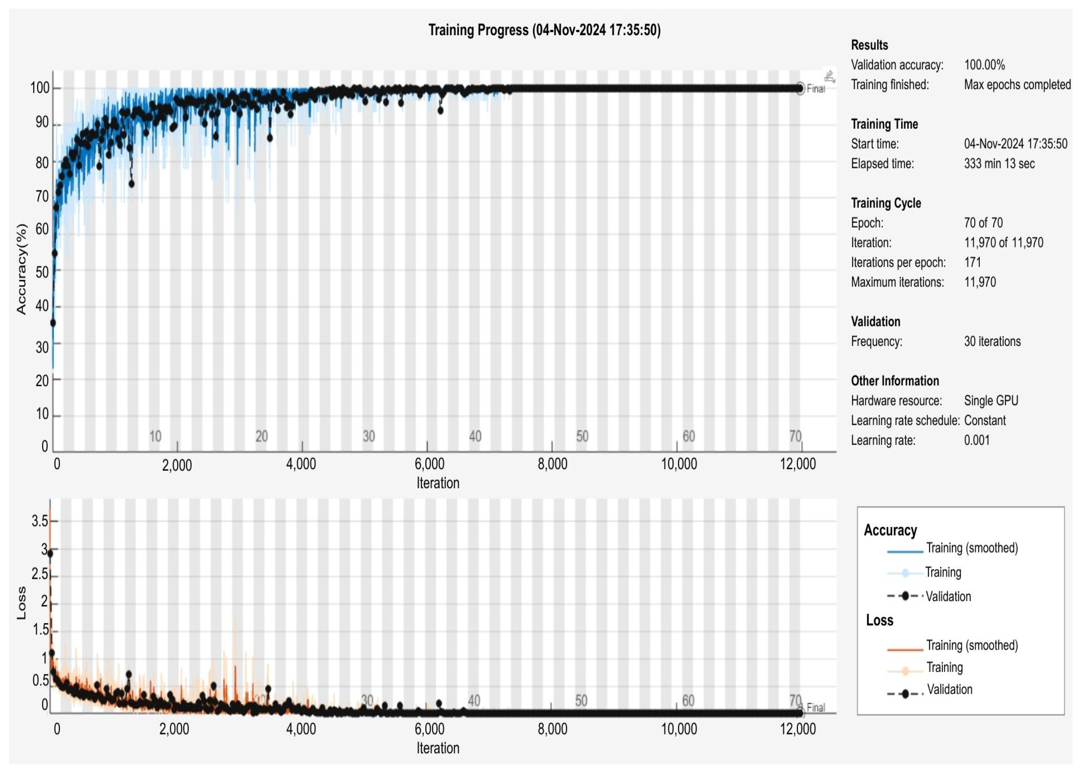
Throughout the nine training iterations, the accuracy values obtained ranged between 84.38% and 88.82%, with individual training accuracies recorded as 86.51%, 88.82%, 87.34%, 84.38%, 85.03%, 87.99%, 87.01%, 87.99%, and 86.68%. Upon completing all training cycles, the final model was constructed by combining the nine trained models, resulting in a final accuracy of 100%. 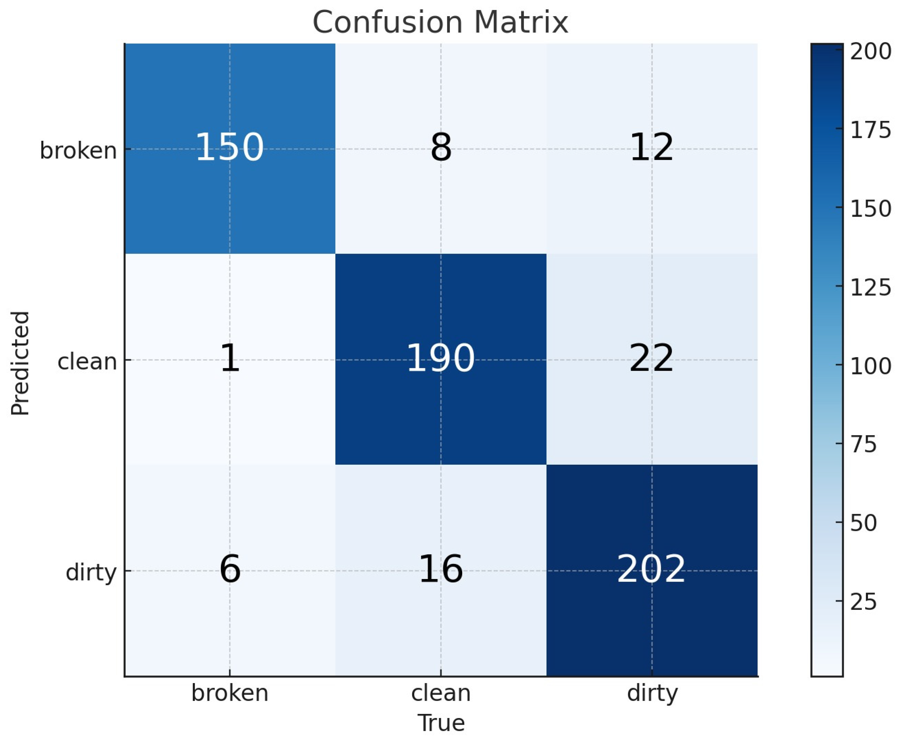The accuracy and loss trends observed throughout the training process are visually represented in Figure 19. At the same time, the confusion matrix, which provides a detailed breakdown of the test results, is presented in Figure 20.

As demonstrated in Figure 19, the data were retrieved from the MATLAB Deep Learning platform. Figure 19 is divided into two sections: the upper section displays the accuracy values, while the lower section presents the loss values. The horizontal axis (x-axis) denotes the number of iterations in the training process, while the vertical axis (y-axis) shows the accuracy and loss values.

In the accuracy graph, the blue color represents the accuracy rates in the training dataset, while the black curve represents the accuracy rates in the validation dataset. The graph illustrates a rapid escalation from the commencement of training, attaining over 90% accuracy following approximately 4000 iterations and stabilizing at the subsequent stages of training, nearing 100% accuracy. The proximity of the training and validation curves suggests that overfitting issues do not afflict the model and that it possesses a high degree of generalization capability.

In the loss graph, the orange color indicates the loss values in the training data, while the black curve represents the loss values in the validation data. The loss values, which are elevated at the commencement of training, rapidly decline to a low level after approximately 2000 iterations and stabilize at the minimum value in the subsequent iterations. This outcome demonstrates that the model exhibits an adequate learning capacity and that the parameters are effectively updated during training.

Consequently, to enhance the clarity of the graphs, the accuracy and loss curves are presented in a larger format with more precise details; axis labels, legends, and visual explanations are incorporated.

In the CNN k-fold training and test results, i.e., accuracy, specificity, and sensitivity, are given in

Table 5. Accuracy, specificity, and sensitivity results for training and testing in CNN k-fold.

	Accuracy	Sensitivity	Specificity
Train	100%	100%	100%
Test	92.86%	89.29%	94.64%

.

Based on the confusion matrix presented in Figure 20, the F1-score, precision, and recall values are detailed in

Table 6. Test results for each class and overall performance in CNN k-fold.

Score of Class	F1-Score	Precision	Recall
class score 0	91.60%	95.54%%	88.23%
class score 1	88.90%	88.78%	89.20%
class score 2	88.22%	85.60%	91.00%
all classes	87.18%	87.18%	87.18%

.

3.6. Comparison of All Models

Considering all the factors discussed, it can be concluded that the three models evaluated in this study—YOLOv8-m, YOLOv9-e, and CNN—demonstrate high classification accuracy in distinguishing between broken, clean, and dirty solar panels. Each model exhibits strong performance metrics, with variations in precision, recall, specificity, and overall efficiency depending on the dataset and training methodology. These results highlight the effectiveness of deep learning-based approaches in automated solar panel inspection, providing a reliable foundation for real-world implementation.

As demonstrated in

Table 7. Precision–recall, F1, precision, recall, accuracy, sensitivity, and specificity results for YOLOv8-m, YOLOv9-e, and CNN k-fold.

Model	Precision–Recall	F1-Score	Precision	Recall	Accuracy	Sensitivity	Specificity
YOLOv8-m	97.10%	93%	100%	100%	97.26%	100%	95.94%
YOLOv9-e	96.80%	92%	100%	100%	95.18%	100%	93.07%
CNN k-fold	-	87.18%	87.18%	87.18%	92.86%	89.29%	94.64%

, the YOLOv8-m model achieves higher accuracy compared to the other algorithms evaluated in this study. Its superior classification performance can be attributed to its advanced feature extraction capabilities, efficient object detection framework, and optimized training process. These factors collectively enable YOLOv8-m to accurately distinguish between broken, clean, and dirty solar panels, making it the most effective model among the three tested approaches. The detailed comparison presented in Table 7 further reinforces its superiority in accuracy and reliability for solar panel classification tasks.

4. Discussion

The findings of this study demonstrate the effectiveness of deep learning models, particularly YOLO-based architectures, in classifying solar panel conditions. The YOLOv8-m model achieved the highest accuracy (97.26%) and specificity (95.94%), outperforming both YOLOv9-e (95.18% accuracy) and the CNN model with k-fold cross-validation (92.86% accuracy). These results align with recent advancements in object detection models, where YOLO variants have shown superior performance in real-time applications due to their optimized architecture for balancing speed and accuracy. For instance, Zhang et al. reported a 91.8% mAP@0.5 for defect detection using YOLOv8, which is consistent with our findings, further validating the robustness of YOLO-based approaches in solar panel inspection tasks [12].

The proposed model performed well, as observed in

Table 8. Comparison of this research with related works.

Author(s)	Method	Accuracy
P. Malik et al. [19]	YOLOv5 and YOLOv9	70.4%
S.E. Droguett et al. [22]	YOLOv9 andYOLOv10	74–73%
Q. B. Phan et al. [16]	YOLOv8	94%
MZ. Ab. Hamid et al. [21]	YOLOv9	96%
SPHERE (Proposed Research)	YOLOv8-m	97.26%

, where similar studies are also mentioned. This comparison highlights its superiority in solar panel defect detection, achieving a higher accuracy (97.26%) compared to other state-of-the-art methods like YOLOv8 (94%) and YOLOv9 (96%). Such advancements underscore the potential of YOLOv8-m as a leading solution for automated inspection systems.

A key strength of this study lies in the use of a novel, proprietary dataset comprising 6079 images under diverse environmental conditions. Unlike publicly available datasets, this dataset was meticulously curated to include variations in lighting, angles, and panel orientations, enhancing its applicability to real-world scenarios. Data augmentation techniques, such as rotation, shifting, and flipping, were critical in addressing class imbalance, particularly for the underrepresented “broken” class. This approach not only improved model generalization but also reduced overfitting risks, as evidenced by the high sensitivity (100%) of YOLOv8-m and YOLOv9-e models.

The superior performance of YOLO models over the CNN can be attributed to their inherent design for object detection tasks. YOLO architectures excel in localizing and classifying objects within images, making them inherently suitable for identifying defects like cracks or dirt on solar panels. In contrast, while the CNN model demonstrated strong generalization through k-fold cross-validation, its lower accuracy (92.86%) highlights the challenges traditional CNNs face in handling spatially complex defects without explicit localization mechanisms. This aligns with Malik et al. (2024), who noted that hybrid models (e.g., CNN-GAN) could enhance performance, suggesting potential avenues for future CNN-based improvements [19].

The developed novel CNN architecture achieved 92.86% accuracy with k-fold cross-validation and produced competitive results compared to similar CNN structures in the literature, despite its low performance compared to YOLO-based models.

Notably, the YOLOv8-m model’s specificity (95.94%) and precision–recall scores (97.10%) indicate its reliability in minimizing false positives, a critical factor for automated inspection systems where misclassifications could lead to unnecessary maintenance costs. The model’s stability during training, as reflected in its consistent loss reduction and validation metrics (Figure 8 and Figure 10), further underscores its suitability for deployment in resource-constrained environments.

The confusion matrix analysis revealed that the ‘dirty’ class was misclassified as ‘broken’. These errors are due to the visual similarity of dark spots to micro-cracks, light reflections creating misleading impressions, and loss of fine detail in low-resolution images. Suggested improvements to address these issues include the following:

• Attention mechanisms such as CBAM to focus the model on critical regions (panel cell boundaries) [51].
• Synthetic data augmentation simulating combinations of dirt and cracks.
• Temperature-based discrimination enhancement by multi-spectral analysis integrating thermal and RGB data.
• Dual-stream CNN architecture that processes textural and structural features in parallel.
• Integration of sub-models highlighting micro-cracks. In addition, it is aimed to reduce false positives by post-processing filtering (hotspot detection) based on thermal data.

These steps can significantly improve the model’s reliability in industrial applications by reducing the error rate.

The primary reason for the superior performance of YOLOv8-m (97.26% accuracy) over YOLOv9-e (95.18% accuracy) is significant disparities in architectural design and feature processing strategies. The YOLOv8-m model has been demonstrated to achieve high levels of accuracy in detecting both minor and complex defects (i.e., micro-cracks) by its CSPDarknet-based backbone structure, multi-scale feature fusion with the SPPF module, and dynamic anchor-free mechanism. In contrast, although YOLOv9-e incorporates advanced techniques such as transformer-based layers and adaptive feature selection, these features increase the risk of overfitting at limited data scales. They may result in the loss of critical details in complex backgrounds (e.g., dirt–shadow blending). Furthermore, the architecture of YOLOv8-m is simpler and more stable, enabling faster convergence in the training process.

In contrast, the gradient-guided optimization of YOLOv9-e increases the computational burden. Consequently, the practice-oriented design (SPPF, dynamic anchor) of YOLOv8-m offers enhanced performance in heterogeneous environments, such as solar panels. In order to unlock the potential of YOLOv9-e, integration with larger datasets or attention mechanisms can be proposed.

In this study, the performance of the CNN model was evaluated using 9-fold cross-validation, while the YOLO models were tested using a fixed data split (70% training, 20% validation, and 10% testing). The direct comparability of these methodologies is questionable. Cross-validation measures have been shown to generalize performance more reliably, whereas fixed splits carry the risk of dependency on a particular data distribution. However, 9-fold cross-validation is not a viable option due to the substantial training times and resource constraints of YOLO models. This finding aligns with the conclusions of analogous studies documented in the extant literature [19].

In order to provide a fair comparison, the fixed division-trained version of the CNN model was also tested, with 92.86% accuracy being obtained. This result is lower than the 97.26% accuracy of YOLOv8-m measured with fixed splitting, thus supporting the architectural superiority of YOLO. Moreover, given the real-time performance (45 FPS) and object localization capabilities of YOLO models, the results obtained with fixed splitting remain valid in practical applications.

However, certain limitations must be acknowledged. The dataset, though diverse, was limited to three classes (broken, clean, and dirty). Expanding the classification to include subcategories of defects (e.g., micro-cracks and delamination) or environmental factors (e.g., snow and shading) could improve practical utility. Additionally, while data augmentation mitigated class imbalance, the relatively smaller size of the “broken” class (2245 images vs. 2130 clean and 1704 dirty) may still introduce subtle biases. Future studies could explore synthetic data generation or adversarial training to further address this issue.

The integration of these models with IoT-enabled autonomous systems, as suggested by Mohammad et al., represents a promising direction for real-time monitoring and maintenance [6]. Such systems could leverage YOLOv8-m’s high accuracy to trigger automated cleaning or repair protocols, significantly enhancing grid stability and energy output efficiency.

The proposed YOLOv8-m model has the potential to offer a practical solution for the automatic inspection of photovoltaic systems through its real-time inference capability, which operates at a rate of 45 frames per second. However, it is imperative to acknowledge the pivotal role that parallel computing and model optimization techniques play in enhancing processing speed in large-scale solar farms and the field of high-resolution drone imagery. To illustrate this point, consider the potential of spatio-temporal models based on deep reinforcement learning (DRL), which can facilitate concurrent processing of the model across multiple Graphics Processing Units (GPUs) or distributed systems [52]. This approach has the potential to markedly reduce latency and optimize resource utilization, particularly in the context of data processing from video streams.

Moreover, drawing inspiration from the research conducted in Travel Demand Forecasting Considering Natural Environmental and Socioeconomic Factors, the present study aims to develop a model that explores the relationship between the geographical distribution of solar panel defects and environmental parameters, such as humidity, temperature, and dust accumulation [53]. Consequently, this approach facilitates proactive prediction of defects and subsequent reduction in maintenance costs.

Using fast spatial–temporal compression algorithms facilitates the instantaneous processing of high-dimensional thermal and visual data collected through drone technology [54]. In particular, techniques employed in traffic flow estimation with complex non-linear patterns can reduce the data size by filtering out superfluous background information in solar panel images. This optimizes the training and inference times of YOLO models while improving energy efficiency on IoT devices.

Integrating these techniques within a hybrid framework will facilitate the sustainable management of photovoltaic systems, exhibiting high accuracy and low latency.

In conclusion, this study underscores the transformative potential of YOLO-based models in solar panel inspection. By combining advanced architectures with robust dataset design, the proposed framework offers a scalable and reliable solution for automating defect detection, thereby contributing to the sustainable management of photovoltaic systems.

The comparison in Table 8 includes the results of different studies using different datasets. Despite being regarded as a methodological limitation, the primary objective of this study is to introduce a novel dataset to the existing literature and to assess the efficacy of deep learning models on this dataset. Most studies in the extant literature utilize datasets with limited diversity or are inaccessible to the public. The proposed SPHERE dataset (6079 images) is characterized by its coverage of various environmental conditions (light, angle, panel orientation), high-resolution samples, real-world scenarios, and SPHERE public access. This distinction renders the model’s performance in real-world applications more dependable.

Nevertheless, the principal contribution of this study is to provide a new dataset and establish a standard benchmark for future research. The 97.26% accuracy of YOLOv8-m obtained in this study on this dataset will be a reference point for future models to be tested using the same set. Moreover, the heterogeneity of the dataset engenders an optimal milieu for assessing model generalization. In conclusion, the present study aims to address a data-driven gap in the field of photovoltaic defect detection and to pave the way for the development of innovative solutions.

5. Conclusions

The main objective of this study was to conduct a comprehensive performance comparison of state-of-the-art deep learning models—YOLOv8, YOLOv9, and CNNs—for classifying solar panel conditions into three categories: broken, clean, and dirty. One of the unique features of this work is the utilization of a novel, proprietary dataset comprising 6079 high-resolution images captured under diverse environmental conditions, which has not been previously employed in any other research. The results demonstrated that the YOLOv8-m model outperformed its counterparts, achieving the highest accuracy (97.26%) and specificity (95.94%) while maintaining 100% sensitivity. These findings directly contribute to advancing automated inspection systems by providing a robust framework for defect detection, which is critical for maintaining grid stability and optimizing solar energy output.

Another key contribution of this study lies in its methodological rigor. By employing advanced data augmentation techniques to address class imbalance and enhance model generalizability, this work establishes a blueprint for handling imbalanced datasets in photovoltaic defect detection. The comparative analysis of YOLO variants and CNNs highlights the superiority of object detection models over traditional classification architectures for spatially complex tasks. This work will increase the efficiency of other studies in the field by offering insights into model selection, dataset design, and augmentation strategies, thereby accelerating the development of reliable AI-driven maintenance systems.

Future research should focus on expanding the dataset to include additional defect categories and environmental factors to improve real-world applicability. Integrating the proposed framework with IoT-enabled autonomous systems for real-time monitoring, as well as exploring hybrid architectures, could further enhance detection accuracy and operational efficiency. By addressing these challenges, this study paves the way for scalable, sustainable solutions that ensure the longevity and reliability of solar energy infrastructure, ultimately supporting global renewable energy goals.