Article

A Two-Stage Local Path Planning Algorithm Based on Sampling and Optimization Methods

1
College of Artificial Intelligence, Nanjing Agricultural University, Nanjing 210031, China
2
School of Robotics, Hunan University, Changsha 410082, China
*
Author to whom correspondence should be addressed.
Appl. Sci. 2025, 15(9), 4876; https://doi.org/10.3390/app15094876
Submission received: 19 March 2025 / Revised: 10 April 2025 / Accepted: 23 April 2025 / Published: 27 April 2025
(This article belongs to the Special Issue New Insights into Intelligent Robotics)

Abstract

:
As the application of mobile robots becomes increasingly widespread, many navigation applications now require more than just obstacle avoidance capabilities. There is a growing demand for robots to follow predetermined global paths. Inspired by stamping technology in the metalworking field, this paper proposes a two-stage local path planning algorithm based on sampling and optimization, termed the path stamping forming algorithm. In the exploration stage, the path stamping forming algorithm finds a preliminary path that avoids obstacles and runs parallel to the global path. The subsequent optimization stage determines the optimal local path that meets specific constraints. Finally, we compared the proposed algorithm with existing advanced navigation algorithms through simulations and experiments, demonstrating its superior performance. The results indicate that the proposed algorithm enables mobile robots to avoid obstacles and follow the global path without the need to re-plan the global path. Compared with the traditional local path planning algorithm, the performance of the proposed algorithm in following the global path is improved by up to 52.71%.

1. Introduction

The rapid development of mobile robots offers extensive possibilities for addressing a variety of tasks. However, achieving autonomous navigation for mobile robots remains a challenging endeavor. One critical factor in ensuring the safe and efficient completion of navigation tasks is local path planning [1,2]. Current local path planning algorithms primarily focus on enabling mobile robots to reach their destinations quickly and safely, often overlooking the significance of the global path in robotic navigation applications. For instance, robots such as disinfection robots [3], vacuum cleaning robots [4], inspection robots [5], and tour guiding robots [6] must operate along designated global paths to perform their tasks effectively. Therefore, this paper focuses on how local path planning algorithms can achieve obstacle avoidance and adherence to the global path in navigation tasks where the global path cannot be arbitrarily altered.
To enable mobile robots to navigate around obstacles while closely following the global path, the core idea of the method proposed in this paper is to simulate the stamping forming technique used in metalworking. Stamping forming involves placing a metal sheet between molds and then applying high pressure with a punch press. This process deforms the metal sheet, shaping it along the indentations of the mold. In the context of local path planning for mobile robots, obstacles are analogous to molds, the global path is analogous to the punch, and the local path is analogous to the metal sheet. By simulating the stamping process, the local path can be shaped to contour around obstacles while adhering to the global path. Therefore, the proposed method is termed the path stamping forming (PSF) algorithm.
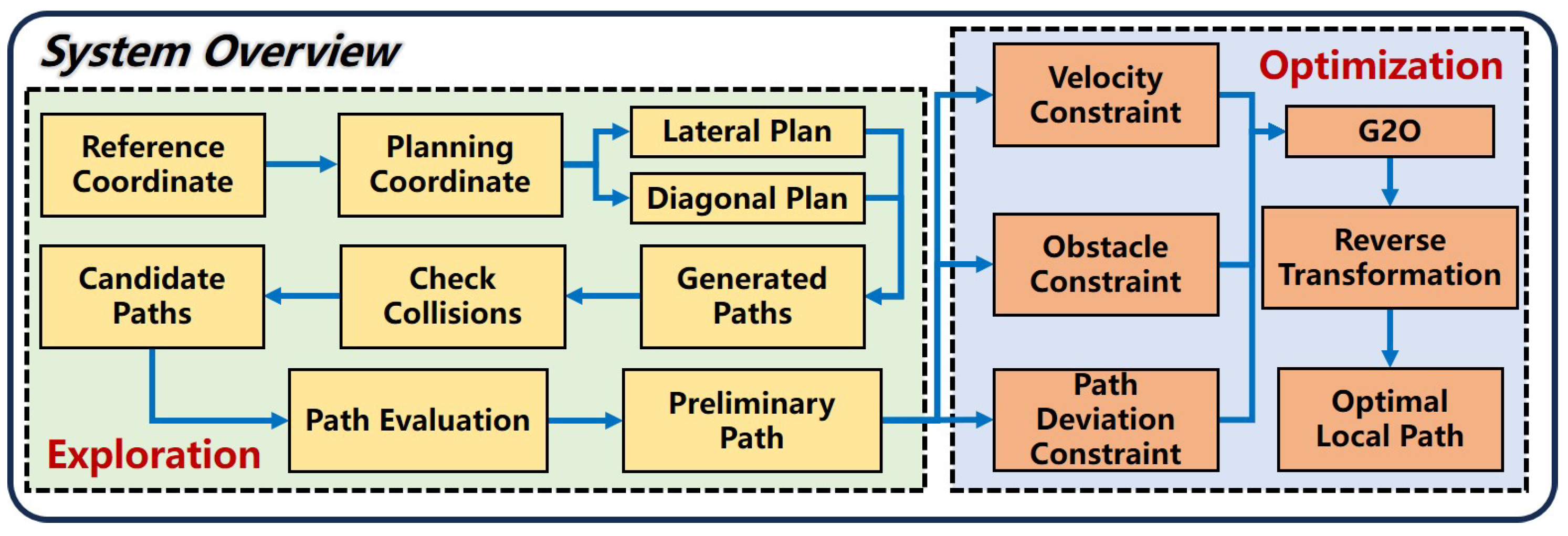
The PSF algorithm is a two-stage local path planning method based on sampling and optimization, as illustrated in 
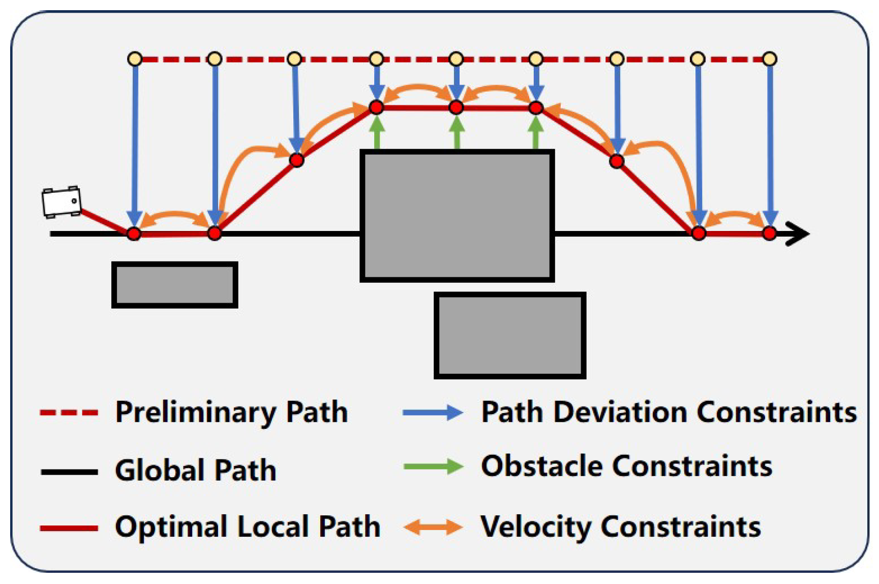
Figure 1. Initially, the PSF algorithm employs a sampling approach to generate a preliminary path that runs parallel to the global path without colliding with obstacles, similar to the initial position of the metal sheet in the stamping process. Subsequently, the PSF algorithm establishes constraints for path deviation, obstacle avoidance, and velocity, similar to the downward pressure exerted by the punch, the resistance from the molds, and the deformation limits of the metal sheet during stamping. Finally, an optimization method is employed to compute the optimal local path that satisfies these constraints.
The contributions of this study are as follows:
1. The PSF algorithm comprehensively considers the significance of the global path in navigation tasks. It ensures that mobile robots can quickly return to the global path after deviating from it and then continue following the global path.
2. During the optimization stage, we only consider obstacles relevant to the global path, rather than all obstacles in the environment. Additionally, we optimize only the longitudinal distance between the mobile robot and the global path, thereby reducing the computational complexity of the optimization process.
3. This paper conducts extensive experiments on the PSF algorithm, comparing its navigation performance with existing advanced navigation algorithms, and demonstrating the superior performance of the PSF algorithm in following the global path. Furthermore, the effectiveness of the PSF algorithm is validated on real robots and in typical tasks.
The rest of this paper is organized as follows. Section 2 reviews the related work. Section 3 presents the proposed path stamping forming algorithm. In Section 4, simulations and experiments illustrate the effectiveness and performance of the proposed algorithm, and finally, Section 5 concludes this paper.

2. Related Work

Currently, local path planning algorithms for mobile robots primarily include multi-path generation and evaluation methods, as well as single-path direct optimization methods.

2.1. Multi-Path Generation and Evaluation Method

The primary idea behind the multi-path generation and evaluation method is to generate a series of possible candidate paths in the configuration space surrounding the mobile robot. Subsequently, for each candidate path, collision risk with the environment, proximity to the goal, smoothness relative to the current velocity, and other metrics are evaluated based on predefined objective or cost functions. Finally, the optimal path is selected to fulfill the local path planning task.
Dynamic window approach (DWA) is one of the most widely used algorithms in local path planning for mobile robots. While DWA can address path planning problems in complex and dynamic environments, its performance in planning local paths is closely related to the number of candidate paths. Therefore, some scholars have proposed improvement methods. For instance, parameter adaptation through fuzzy logic [7,8,9] and learning methods [10,11] has been suggested. Additionally, deep learning methods have been proposed to generate feasible trajectory sequences omnidirectionally as auxiliary candidate trajectories [12]. Semantic maps were generated by semantic simultaneous localization and mapping algorithms for robot planning under uncertainties [13]. However, approaches based on deep learning or planning with semantic maps require a lot of computing resources, resulting in problems such as high computational complexity and weak generalization ability. There have also been improvements in sampling methods to make them applicable to systems with uncertainty [14]. In the field of autonomous driving, the frenet optimal trajectory (FOT) algorithm proposed by Werling et al. [15] adopts a similar approach. This algorithm samples a series of candidate terminal states and fits smooth curves connecting the current state to these candidate states to plan the vehicle’s trajectory. Subsequently, an evaluation function considering factors such as safety and comfort is used to select the optimal trajectory [16].

2.2. Single-Path Direct Optimization Method

The single-path direct optimization method typically transforms the local path planning problem into an optimization problem. These algorithms usually consider multiple factors, such as path length, the robot’s kinematic constraints, distance from obstacles, smoothness of speed and acceleration, and travel time. By integrating these factors, the algorithm can generate paths that are safe, comfortable, and efficient.
In traditional solutions, a feasible initial path is first generated by a path planner. This initial path is then refined through optimization algorithms. For example, initial paths generated by planners based on ant colony optimization [17,18], rapidly exploring random trees [19], artificial potential fields [20], particle swarm optimization (PSO) [21], and Bézier curves [22] have been optimized further. However, in dynamic environments, these methods require the initial path to be regenerated, necessitating the design of re-planning strategies to ensure the robot follows the global path. The time-elastic-band (TEB) algorithm proposed by Rösmann et al. [23,24] optimizes the entire solution space to ensure the local path is optimal under given constraints. The main idea of the TEB algorithm is to treat the global path as an elastic band that deforms under internal and external forces, adjusting the global path based on the position and shape of obstacles. Different constraint parameters can be set to adapt to the complexity of the scenario. Therefore, the TEB algorithm is also one of the most widely applied methods.
Although the single-path direct optimization method effectively addresses multi-objective optimization problems and can more easily find the optimal path solution compared to multi-path generation and evaluation methods, it also requires substantial computational resources and time to find the optimal solution. If inappropriate optimization algorithm parameters and cost function weights are selected, the algorithm’s performance and results may be adversely affected. This can lead to issues such as failure to converge or becoming trapped in local optima.

3. Proposed Method

3.1. Overview

In this study, a combined sampling and optimization approach is adopted for local path planning of mobile robots, as depicted in Figure 2. The PSF algorithm consists of two stages: the exploration stage and the optimization stage. During the exploration stage, a coordinate transformation is performed on the mobile robot. Then, a set of path candidates is generated through lateral planning and diagonal planning. Subsequently, the candidate paths that do not collide with obstacles in the environment are retained and scored. The candidate path with the highest score is selected as the preliminary path. In the optimization stage, the preliminary path undergoes further optimization. Initially, a factor graph is constructed, with vertices representing the preliminary path and edges representing path deviation constraints, obstacle constraints, and velocity constraints. Next, the factor graph is solved using the general graphic optimization (G2O). Finally, the coordinates are inversely transformed to generate the optimal local path.
Due to the typical navigation tasks of mobile robots, which involve global path planning in grid maps using algorithms such as Dijkstra’s and A*, the global path is inevitably composed of straight-line segments. Therefore, this study only considers local path planning under this general scenario, where the global path consists of straight-line segments.

3.2. Exploration Stage

3.2.1. Coordinate Transformation

The core idea of the PSF algorithm is to minimize the deviation between the local path and the global path, meaning that the distance between corresponding points on the global and local path should be as small as possible. Therefore, the distance between the local path and the global path is a crucial parameter in the PSF algorithm. To better represent the relationship between any point in space and the global path, its position will be described based on its lateral distance and longitudinal distance from the global path, as illustrated in Figure 3.
Taking the starting point ( x 0 , y 0 ) of the global path as the origin, a planning coordinate system is established. The horizontal axis aligns with the direction of the global path, while the vertical axis aligns with its normal direction. Therefore, the coordinates of any position in the planning coordinate system represent the lateral and longitudinal distances from the point to the global path.
First, the reference coordinate system is transformed into the planning coordinate system:
θ = a r c t a n y 1 y 0 x 1 x 0
c o s θ s i n θ s i n θ c o s θ · x i x 0 y i y 0 = s i d i
where θ in (1) is the rotation angle, representing the angle between the global path and the x-axis of the reference coordinate system. ( x i , y i ) in (2) denotes the coordinates to be transformed, while ( s i , d i ) represents the transformed coordinates. When ( x i , y i ) lies on the global path, d i equals 0.
Therefore, the coordinates of any point in the reference coordinate system can be represented by its lateral and longitudinal distances from the global path, denoted as ( s , d ) . The objects scanned by the LiDAR are also transformed into this coordinate system, with the set of LiDAR point positions represented as ( L s i , L d i ) .

3.2.2. Candidate Paths

The candidate paths are a set of paths parallel to the global path and free from collisions with obstacles. These candidate paths are generated using the lateral planning and the diagonal planning, as illustrated in Figure 4.
In lateral planning, the robot is first sampled at a constant velocity. Assuming the robot moves forward in a straight line at the maximum velocity v m a x within a specified time interval Δ t , the maximum distance it travels is S m a x . This allows us to generate a series of discrete position points, forming a lateral path. Next, positions are sampled on both sides of the global path at a fixed width W. Assume that N paths are sampled on each side. Consequently, a total of 2 × N lateral paths can be generated on both sides of the global path. The formula for generating the nth lateral path is given as
j m a x = S m a x v m a x · Δ t
{ H s j n , H d j n } = ( s 0 + j · v m a x · Δ t , W · ( n N ) ) , j ( 1 , j m a x )
where ( s 0 , d 0 ) in (4) is the coordinate of the robot in the planning coordinate system. { H s j n , H d j n } is the position set of the nth lateral path. j represents the position point index of the lateral path, and j m a x in (3) is the total number of position points in the lateral planning.
At the same time, there is a diagonal path between the robot and the first sampling point in each lateral path. Therefore, the diagonal planning needs to be performed. The width R of the robot is used as the distance sampling value. Thus, a diagonal path between the robot and the nth lateral path is generated. The formula for generating the nth diagonal path is expressed as
α = a r c t a n H d 1 n d 0 H s 1 n s 0
k m a x = ( H s 1 n , H d 1 n ) ( s 0 , d 0 ) / R
{ D s k n , D d k n } = ( s 0 + k · c o s α · R , d 0 + k · s i n α · R ) , k ( 1 , k m a x )
where α in (5) is the intermediate variable. { D s k n , D d k n } in (7) is the position set of the nth diagonal path. k represents the position point index of the diagonal path, and k m a x in (6) is the total number of position points of the diagonal planning.
The lateral path position sets { H s j n , H d j n } and the diagonal path position sets { D s k n , D d k n } together form the generation path sets { G s m n , G d m n } , as illustrated by the dashed trajectories in Figure 4.
Next, the obstacle collision detection needs to be performed on the generation path sets, where the paths that collide with obstacles are discarded. The discarded paths can be determined as
m m a x = j m a x + k m a x
{ G s m n , G d m n } ( L s i , L d i ) < R , m ( 1 , m m a x )
If any position of the nth generation path satisfies the above equation, that path is considered a discarded path, depicted as the gray dashed trajectories in Figure 4. The lateral paths remaining in the final set of generation paths are considered candidate paths { C s m n , C d m n } , illustrated as the yellow and red dashed trajectories in Figure 4.

3.2.3. Preliminary Path

The preliminary path is a parallel line that is closest to the global path and without collision. In order to find this preliminary path among candidate paths, they need to be scored. Then, the candidate path closest to the global path is selected as the preliminary path. The longitudinal distance in lateral planning and the longitudinal distance of the robot are used as the evaluation criteria for scoring. Therefore, the scoring formula for the nth candidate path is as follows:
s c o r e = d 1 n d 0
All candidate paths are scored, where the candidate path with the lowest score becomes the preliminary path, as depicted by the red dashed trajectory in Figure 4. The preliminary path position set is represented as B = { P s j , P d j } .

3.3. Optimization Stage

The core idea of the PSF algorithm in the optimization stage is to simulate the stamping forming technique. Initially, the pressure is applied to the preliminary path along the direction of the global path, gradually making it closer to the global path. In this process, the path encounters resistance generated by obstacles, causing deformation. Additionally, due to the limitation of the robot’s velocity, the preliminary path will not undergo extensive deformations. Therefore, the preliminary path can be adjusted in real time and multi-objective-optimized from three aspects: the distance between the preliminary path and the global path, the distance between the preliminary path and obstacles, and the kinematic constraints of the robot’s motion. This enables the generation of an optimal local path, denoted as B * . B * can be obtained by minimizing a weighted nonlinear least squares cost function. The cost function consists of the objective T and penalty P, expressed as
B * = arg min B e γ e f e ( B ) , e { T , P }
where f T represents the objective function concerning constraints on the deviation of the local path, and f P represents the penalty function regarding constraints on obstacles and velocity. γ e denotes the weights among these terms. The G2O framework can be utilized to solve the above functions [23].

3.3.1. Path Deviation Constraint

At the optimization stage, the preliminary path needs to be close to the global path due to the coordinate transformation steps described in Section 3.2. Therefore, we can easily describe the approximation of the preliminary path and the global path by the longitudinal coordinate of the preliminary path. The target function of the path deviation constraint is described as
f d e v = min B j = 1 j m a x d j

3.3.2. Obstacle Constraint

In the planning coordinate system, the expression of obstacle information can be simplified. This is because the method only needs to consider whether the local path points are between the obstacles and the global path. First, all laser points between the preliminary path and the global path are retained. These laser points represent the relevant obstacles in the optimization process. Next, only the laser points with the maximum longitudinal distance under the same lateral distance are retained. These laser points can describe the obstacle information and are denoted as obstacle laser points ( O s i , O d i ) . These laser points can be used to determine whether the local path contacts obstacles. The penalty function of the obstacle constraint can be expressed as
f o b s = O d i d j + ε , s j ε < o b s i < s j + ε 0 , e l s e
where ε represents the expansion parameters of obstacles.

3.3.3. Velocity Constraint

During the robot’s movement, it is also necessary to ensure that the local path meets kinematic constraints. Since this paper considers only a differential-drive robot, the constraint is applied solely to the velocity. The velocity constraint ensures that the speed between any two local path points is less than the robot’s maximum velocity v m a x . The penalty function of the velocity constraint can be expressed as
v = ( s j + 1 , d j + 1 ) ( s j , d j ) Δ t
f v e l = v v m a x , v > v m a x 0 , e l s e

3.3.4. Reverse Transformation

After solving (11) using G2O, the optimal local path B * = { s ^ i , d ^ i } can be obtained. However, since B * is still in the planning coordinate system, a coordinate transformation is required to return it to the reference coordinate system. The formula for coordinate transformation is expressed as
x ^ i y ^ i 1 = c o s θ s i n θ x 0 s i n θ c o s θ y 0 0 0 1 · s ^ i d ^ i 1
where ( x ^ i , y ^ i ) represents the coordinates of the optimal local path in the reference coordinate system.

4. Simulations and Experiments

4.1. Simulations

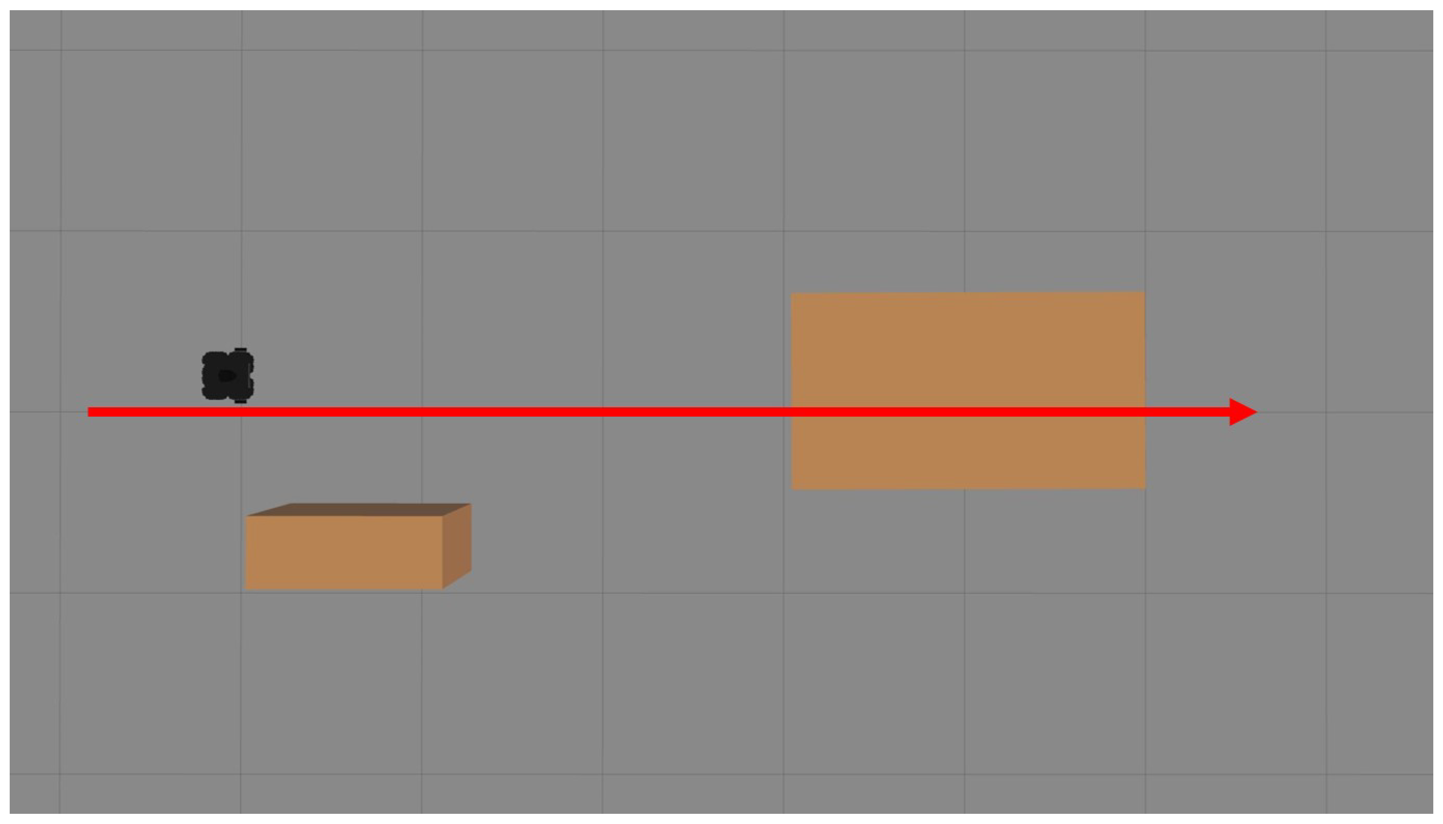
To validate the performance of the PSF algorithm, simulations were conducted using the Gazebo 11 virtual simulation software in Ubuntu 20.04. The TurtleBot3 Waffle model was employed as the mobile robot. A straight global path of 8 m in length was utilized, with two obstacles placed along its trajectory. The initial coordinates of the robot relative to the starting point of the global path were ( 0.5 , 0.2 ) . The simulation was performed on a system with the following specifications: Ubuntu 20 operating system, Intel i5-12 processor, and 16 GB of RAM. The simulation environment is illustrated in Figure 5. The parameters of the PSF algorithm are shown in Table 1.
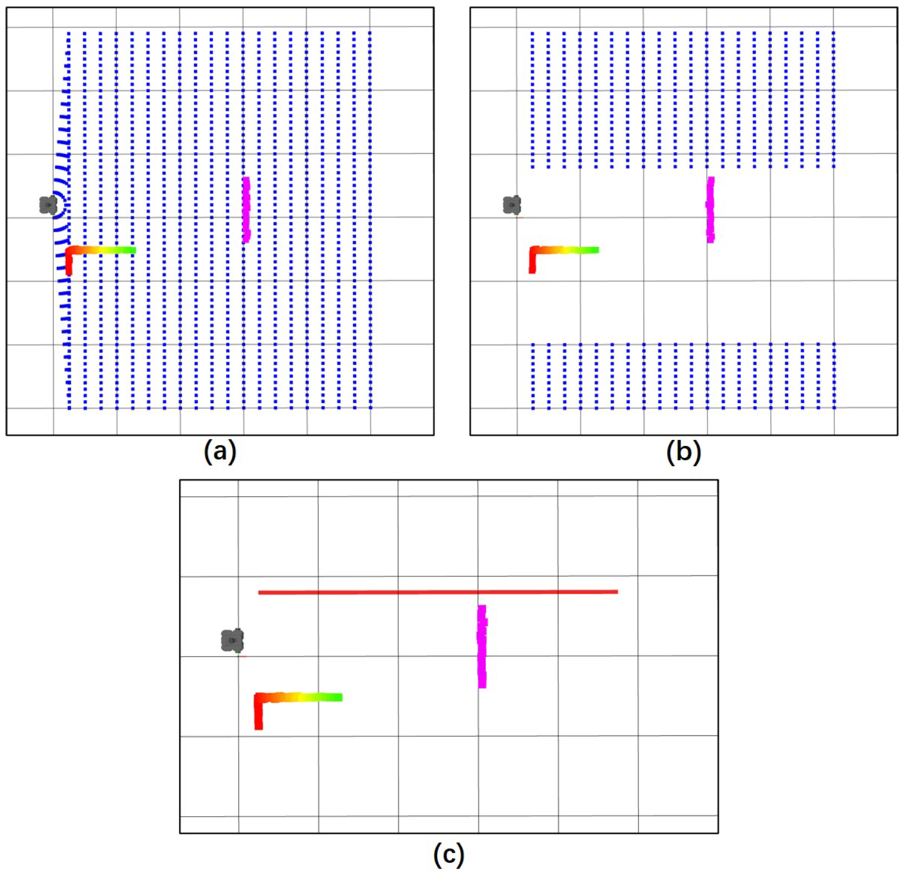
The simulation results of the exploration stage of the PSF algorithm are shown in Figure 6. It can be seen that the exploration stage of the PSF algorithm can easily find a preliminary path that is closest to the global path and does not collide with the obstacles.
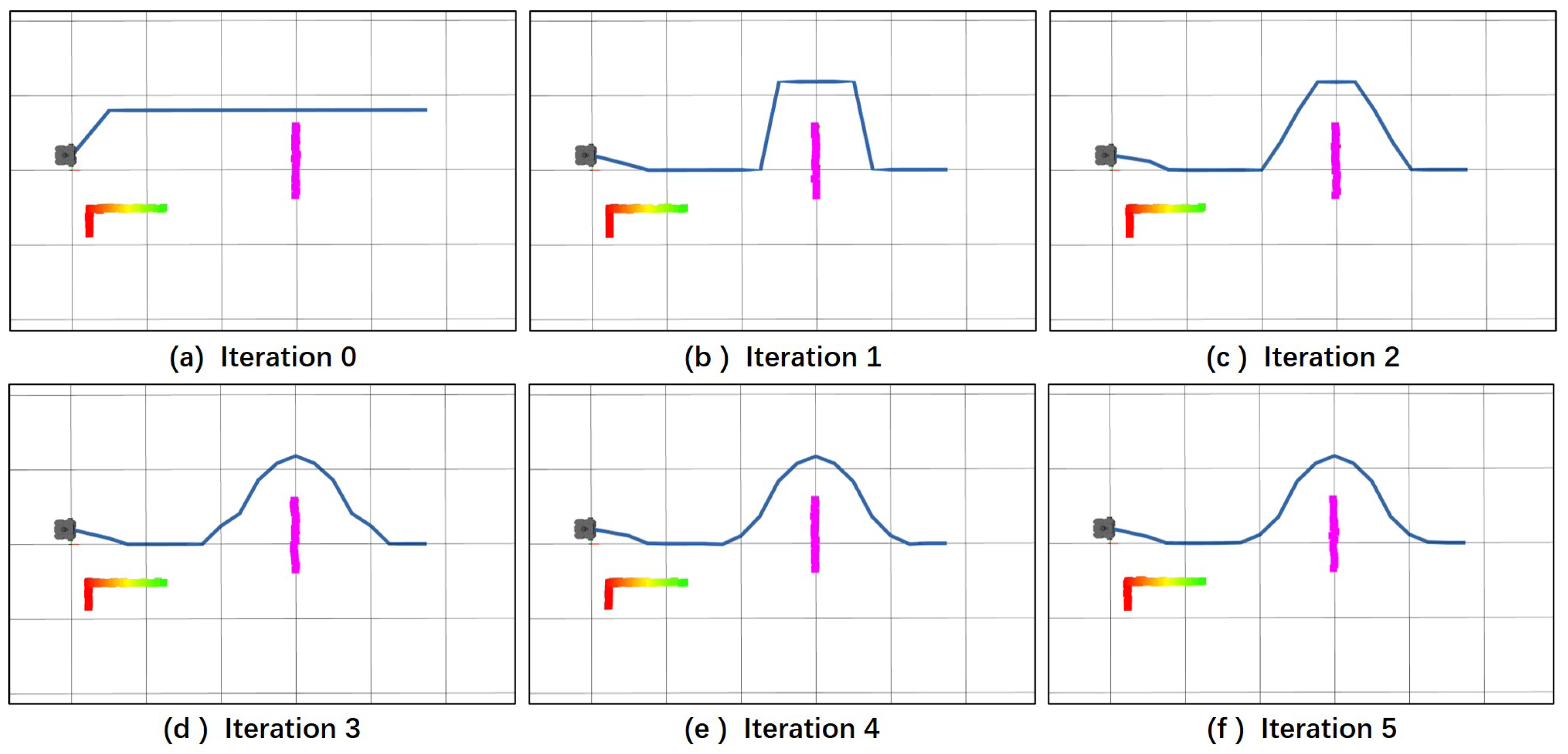
The optimization process during the PSF algorithm optimization stage is depicted in Figure 7. Upon the first iteration of preliminary path optimization, deviations from constraints cause the initial path to deform towards the global path, while obstacle constraints prevent the deformation of the preliminary path around obstacles. As the number of optimization iterations increases, the influence of velocity constraints on the preliminary path gradually intensifies. By the fifth iteration, the optimization algorithm has converged, yielding the optimal local path. It can be observed that due to the PSF algorithm’s optimization solely focusing on longitudinal distance, the algorithm achieves convergence within a short timeframe. Furthermore, obstacle selection is applied, retaining only relevant obstacles, significantly enhancing the efficiency of local path planning.

4.2. Comparative Simulations

In the comparative simulations, the move_base framework in ROS was utilized for navigation. The comparative algorithms included the dwa_local_planner and teb_local_planner packages within move_base. The navigation parameters were selected from the parameter files officially provided for TurtleBot. This study primarily focuses on how to avoid obstacles in the environment using a local path planning algorithm while ensuring that the global path remains unchanged. Additionally, the local path must closely adhere to the global path. It is important to note that the global_planner in move_base performs global path planning at a certain frequency or re-plans when local path planning fails. Consequently, the default global_planner in move_base does not align with the problem addressed in this study.
Therefore, a global_planner_plugin [25] with two modes was developed. One mode generates a straight-line path between the robot’s position and the target point. This mode prioritizes the robot reaching the target directly and is thus referred to as the “Goal” mode. The other mode first plans a perpendicular path from the robot’s position to the global path, then plans a straight-line path from the intersection point to the target point. This mode prioritizes the robot reaching the global path first and is therefore referred to as the “Path” mode.
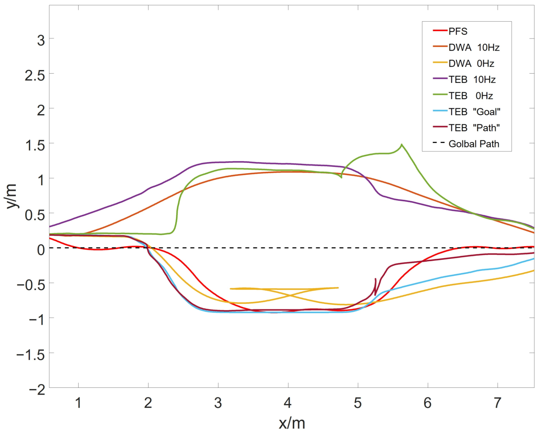
In the comparative simulations, three sets of trajectory comparisons were conducted. To ensure fair comparisons, the parameters’ comparative algorithms followed the empirical selection (without altering the official parameters), and the parameters were tested to achieve a favorable performance. The first and second sets utilized traditional navigation methods for mobile robots, specifically the global_planner combined with either the dwa_local_planner or teb_local_planner. Initially, the global_planner’s planning frequency was set to 10 Hz. Subsequently, the planning frequency was changed to 0 Hz, meaning that the global path was planned only once. The third set of simulations employed our global_planner_plugin to validate the obstacle avoidance and global path-following capabilities of traditional local planners. Since the DWA algorithm predicts the potential trajectories of the mobile robot within a forward simulation time for obstacle avoidance, it was found during actual testing that DWA has limited obstacle avoidance capability when the global path remains unchanged. Therefore, in the third set of simulations, only the TEB algorithm was tested. The simulation results are illustrated in Figure 8.
The simulation results show that the PSF algorithm performs best in following the global path. When the robot deviates from the global path or obstacle avoidance ends, it can reach the global path in a shorter distance. The other two algorithms show different performances in different navigation modes. The errors with the global path are shown in Table 2.
It is evident that under traditional navigation modes, both local path planning algorithms can achieve smooth movement and obstacle avoidance for the mobile robot. However, their local planning capabilities rely on the paths planned by the global_planner. When using the global_planner_plugin, the TEB algorithm exhibited good robustness. In the “Path” mode, the robot prioritized moving toward the global path even after obstacle avoidance. However, since the goal of the TEB algorithm is to plan the shortest possible path in terms of time, its performance in following the global path is not as excellent as that of the PSF algorithm.

4.3. Real Robot Experiments

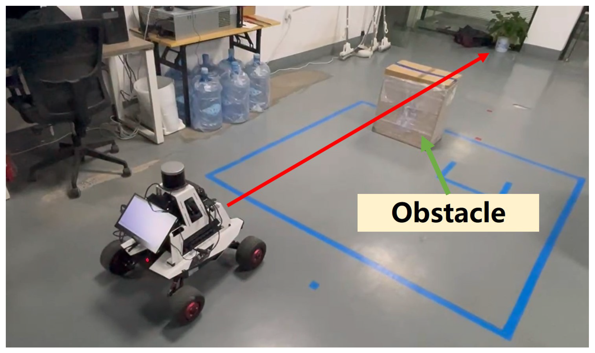
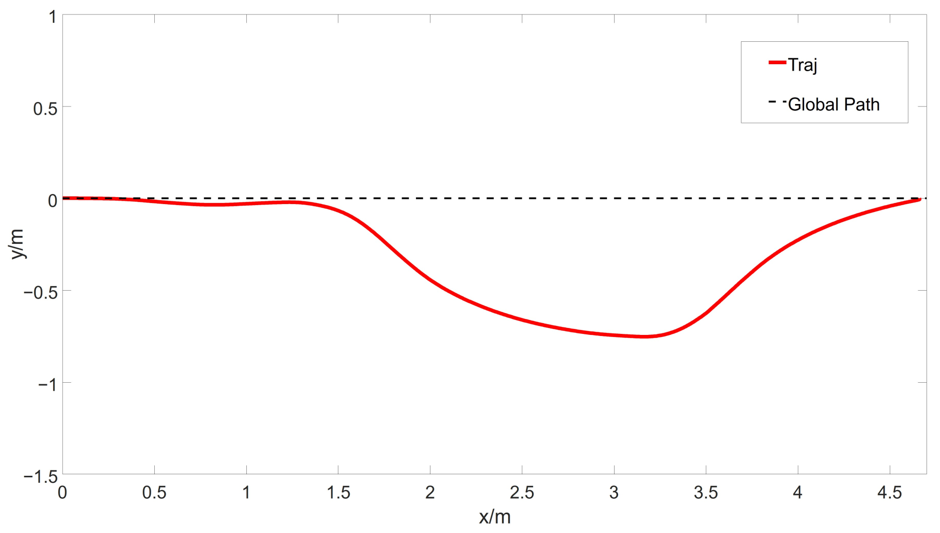
For the final validation experiment, tests were conducted using a Scout Mini robot platform. The same processor used in the simulation experiment was employed. A 5 m global path was designated, and a 30 cm × 20 cm × 50 cm obstacle was placed along this path. The experimental environment is depicted in Figure 9.
The experimental results, as illustrated in Figure 10, show that the experiments on the real robot are consistent with the simulation results. Additionally, the test environment better reflects the real scene of robot operation. The results demonstrate the effectiveness of the PSF algorithm in complex and confined environments.
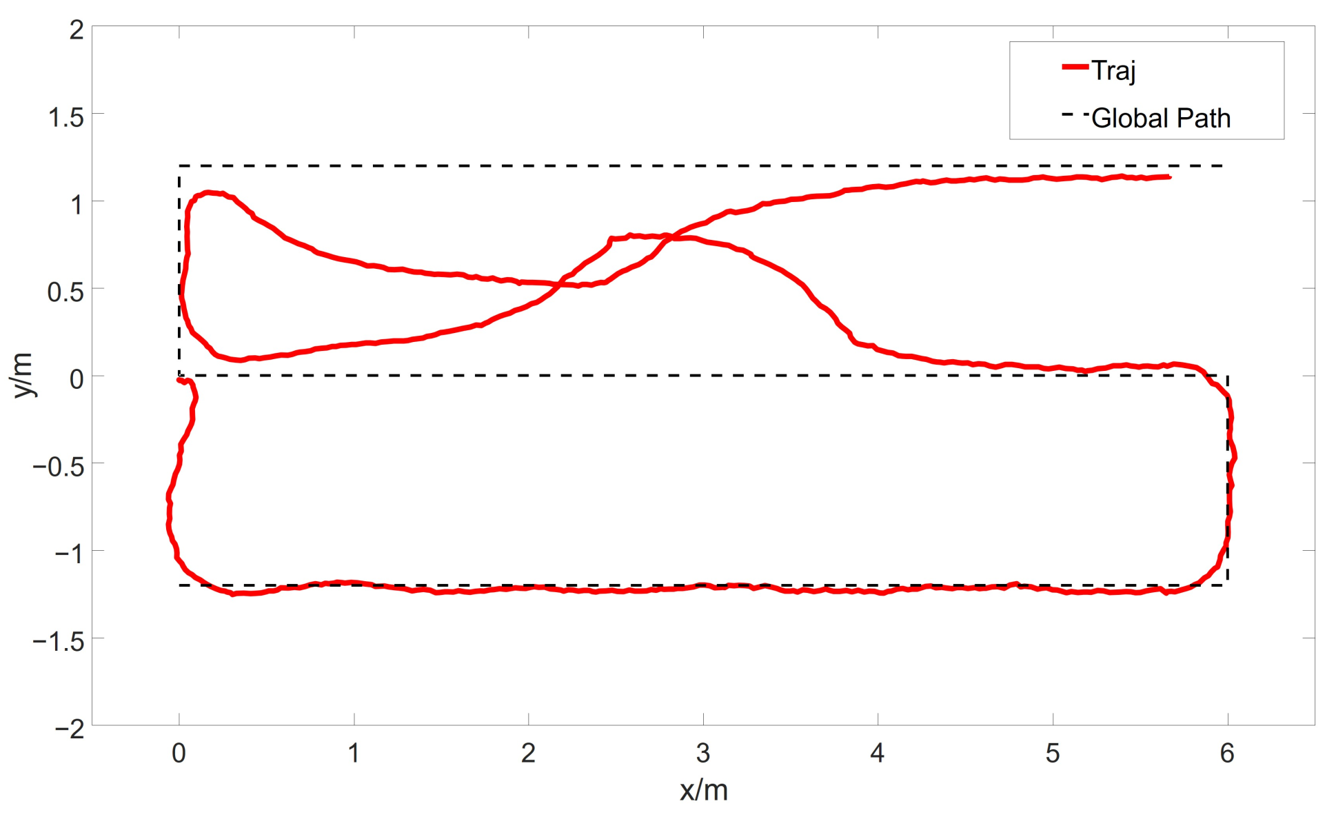
Furthermore, verification experiments on typical tasks were conducted using the PSF algorithm. These tasks resemble the operational tasks of vacuum cleaning robots and disinfection robots, requiring traversal of the environment via a zigzag path. The experimental environment and global path are depicted in Figure 11.
The robot departs from the origin and first reaches the starting point of the global path. It then traverses five segments of the path to reach the endpoint. Due to cumulative errors in odometry, there may be some influence on local planning. Therefore, for typical task experiments, we utilized high-precision laser odometry. This resulted in minor oscillations in the robot’s motion trajectory. The experimental results are shown in Figure 12.
It is evident that the robot, while achieving obstacle avoidance during typical tasks, also swiftly returns to the global path. Throughout this process, the robot ensures that its local path adheres to kinematic constraints. Thus, the PSF algorithm can meet the task requirements of various mobile operation robots, including reconnaissance robots, guiding robots, floor-cleaning robots, and disinfection robots. It is worth noting that this paper focuses exclusively on relatively simple global paths. Currently, the proposed PSF algorithm does not support navigation tasks involving curved global paths. However, in future work, the PSF algorithm can be extended to accommodate curved global paths by using a transformation based on the Frenet coordinate system.

5. Conclusions

This paper presented a path stamping forming algorithm to decouple the local path planning problem into front-end sampling-based search and back-end trajectory optimization. During the exploration stage, the planning coordinate transformation was established, and a collision-free preliminary path was searched. In the optimization stage, several constraints from the path deviation, the obstacle, and the velocity were considered. Then, an optimal and safe local path was generated to adhere to kinematic constraints. Comparative simulations and real-world experiments were conducted to validate the effectiveness and performance of the proposed planning algorithm. This paper considered relatively simple global paths, where the proposed algorithm cannot support navigation tasks involving curved global paths. Therefore, in future work, the proposed algorithm can be extended to accommodate curved global paths by using a transformation based on the Frenet coordinate system, especially in structured environments that involve challenges such as avoiding corners, traversing ramps, and other complex features.

Author Contributions

Conceptualization, Y.L., F.H. and X.Z.; methodology, Y.L. and F.H.; software, Y.L.; validation, Y.L. and X.Z.; formal analysis, Y.L.; investigation, Y.L.; resources, F.H.; data curation, Y.L.; writing—original draft preparation, Y.L.; writing—review and editing, F.H. and X.Z.; visualization, Y.L.; supervision, F.H.; project administration, F.H. All authors have read and agreed to the published version of the manuscript.

Funding

This research received no external funding.

Institutional Review Board Statement

Not applicable.

Informed Consent Statement

Not applicable.

Data Availability Statement

The original contributions presented in this study are included in the article. Further inquiries can be directed to the corresponding author.

Conflicts of Interest

The authors declare no conflicts of interest.

References

  1. Xu, X.; Li, X.; Chen, N.; Zhao, D.; Chen, C. Autonomous Obstacle Avoidance with Improved Deep Reinforcement Learning Based on Dynamic Huber Loss. Appl. Sci. 2025, 15, 2776. [Google Scholar] [CrossRef]
  2. Baek, Y.; Park, J.K. Fast Path Generation Algorithm for Mobile Robot Navigation Using Hybrid Map. Appl. Sci. 2025, 15, 2414. [Google Scholar] [CrossRef]
  3. Yi, J.; Zhang, H.; Mao, J.; Chen, Y.; Zhong, H.; Wang, Y. Review on the COVID-19 pandemic prevention and control system based on AI. Eng. Appl. Artif. Intell. 2022, 114, 105184. [Google Scholar] [CrossRef] [PubMed]
  4. Ramesh, A.; Rameshkumar, V.; Ragabharathi, A.; Sowndar, K.; Sivakumar, P. A survey on smart vacuum learning robot. In Proceedings of the 2023 9th International Conference on Advanced Computing and Communication Systems (ICACCS), Coimbatore, India, 17–18 March 2023; Volume 1, pp. 923–926. [Google Scholar]
  5. Zhang, T.; Dai, J. Electric power intelligent inspection robot: A review. J. Phys. Conf. Ser. 2021, 1750, 012023. [Google Scholar] [CrossRef]
  6. Bose, D.; Mohan, K.; Meera, C.S.; Yadav, M.; Saini, D.K. Review of autonomous campus and tour guiding robots with navigation techniques. Aust. J. Mech. Eng. 2023, 21, 1580–1590. [Google Scholar] [CrossRef]
  7. Xiang, L.; Li, X.; Liu, H.; Li, P. Parameter fuzzy self-adaptive dynamic window approach for local path planning of wheeled robot. IEEE Open J. Intell. Transp. Syst. 2022, 3, 1–6. [Google Scholar] [CrossRef]
  8. Abubakr, O.A.; Jaradat, M.A.; Abdel-Hafez, M.F. Intelligent optimization of adaptive dynamic window approach for mobile robot motion control using fuzzy logic. IEEE Access 2022, 10, 119368–119378. [Google Scholar] [CrossRef]
  9. Fan, J.; Huang, N.; Huang, D.; Kong, Y.; Chen, Z.; Zhang, F.; Zhang, Y. An improved path planning algorithm with adaptive parameters and predictions. IEEE Syst. J. 2023, 17, 4911–4921. [Google Scholar] [CrossRef]
  10. Yang, D.; Su, C.; Wu, H.; Xu, X.; Zhao, X. Construction of novel self-adaptive dynamic window approach combined with fuzzy neural network in complex dynamic environments. IEEE Access 2022, 10, 104375–104383. [Google Scholar] [CrossRef]
  11. Kobayashi, M.; Zushi, H.; Nakamura, T.; Motoi, N. Local path planning: Dynamic window approach with q-learning considering congestion environments for mobile robot. IEEE Access 2023, 11, 96733–96742. [Google Scholar] [CrossRef]
  12. Jiang, D.; Du, L.; Li, S.; Wang, M.; Zhang, H.; Chen, X.; Sun, Y. An improved dynamic window approach based on reinforcement learning for the trajectory planning of automated guided vehicles. IEEE Access 2024, 12, 36016–36025. [Google Scholar] [CrossRef]
  13. Kantaros, Y.; Kalluraya, S.; Jin, Q.; Pappas, G.J. Perception-based temporal logic planning in uncertain semantic maps. IEEE Trans. Robot. 2022, 38, 2536–2556. [Google Scholar] [CrossRef]
  14. Yasuda, S.; Kumagai, T.; Yoshida, H. Safe and efficient dynamic window approach for differential mobile robots with stochastic dynamics using deterministic sampling. IEEE Robot. Autom. Lett. 2023, 8, 2614–2621. [Google Scholar] [CrossRef]
  15. Werling, M.; Ziegler, J.; Kammel, S.; Thrun, S. Optimal trajectory generation for dynamic street scenarios in a Frenét Frame. In Proceedings of the 2010 IEEE International Conference on Robotics and Automation, Anchorage, AK, USA, 3–7 May 2010; pp. 987–993. [Google Scholar]
  16. Yu, Z.; Zhu, M.; Chen, K.; Chu, X.; Wang, X. LF-Net: A learning-based Frenet planning approach for urban autonomous driving. IEEE Trans. Intell. Veh. 2024, 9, 1175–1188. [Google Scholar] [CrossRef]
  17. Yang, H.; Qi, J.; Miao, Y.; Sun, H.; Li, J. A new robot navigation algorithm based on a double-layer ant algorithm and trajectory optimization. IEEE Trans. Ind. Electron. 2019, 66, 8557–8566. [Google Scholar] [CrossRef]
  18. Bueno-Ferrer, Á.; De Pablo Valenciano, J.; De Burgos Jiménez, J. Unveiling the potential of metaheuristics in transportation: A path towards efficiency, optimization, and intelligent management. Infrastructures 2025, 10, 4. [Google Scholar] [CrossRef]
  19. Wang, J.; Meng, M.Q.H.; Khatib, O. EB-RRT: Optimal motion planning for mobile robots. IEEE Trans. Autom. Sci. Eng. 2020, 17, 2063–2073. [Google Scholar] [CrossRef]
  20. Yang, J.; Zhang, H.; Ning, P. Path planning and trajectory optimization based on improved apf and multi-target. IEEE Access 2023, 11, 139121–139132. [Google Scholar] [CrossRef]
  21. Petrovic, A.; Damaševičius, R.; Jovanovic, L.; Toskovic, A.; Simic, V.; Bacanin, N.; Zivkovic, M.; Spalević, P. Marine vessel classification and multivariate trajectories forecasting using metaheuristics-optimized eXtreme gradient boosting and recurrent neural networks. Appl. Sci. 2023, 13, 9181. [Google Scholar] [CrossRef]
  22. Mazen, A.; Faied, M.; Krishnan, M. Optimal kinodynamic trajectory planner for mobile robots in an unknown environment using Bézier contours. IEEE Access 2024, 12, 8655–8667. [Google Scholar] [CrossRef]
  23. Rösmann, C.; Feiten, W.; Woesch, T.; Hoffmann, F.; Bertram, T. Trajectory modification considering dynamic constraints of autonomous robots. In Proceedings of the ROBOTIK 2012; 7th German Conference on Robotics, Munich, Germany, 21–22 May 2012; pp. 1–6. [Google Scholar]
  24. Rösmann, C.; Feiten, W.; Wösch, T.; Hoffmann, F.; Bertram, T. Efficient trajectory optimization using a sparse model. In Proceedings of the 2013 European Conference on Mobile Robots, Barcelona, Spain, 25–27 September 2013; pp. 138–143. [Google Scholar]
  25. Alajlan, M.; Koubâa, A. Writing global path planners plugins in ROS: A tutorial. In Robot Operating System (ROS): The Complete Reference (Volume 1); Springer International Publishing: Berlin/Heidelberg, Germany, 2016; pp. 73–97. [Google Scholar]
Figure 1. The framework of PSF local path planning method.
Applsci 15 04876 g001
Figure 2. System overview of PSF.
Applsci 15 04876 g002
Figure 3. Transforming the reference coordinate system to the planning coordinate system.
Applsci 15 04876 g003
Figure 4. The process of obtaining candidate paths.
Applsci 15 04876 g004
Figure 5. Gazebo simulation environment.
Applsci 15 04876 g005
Figure 6. Simulation results of the exploration stage. (a) Generated paths. (b) Candidate paths. (c) Preliminary path.
Applsci 15 04876 g006
Figure 7. Simulation results of the optimization stage.
Applsci 15 04876 g007
Figure 8. The results of the comparative simulation.
Applsci 15 04876 g008
Figure 9. The experimental environment and robot platform.
Applsci 15 04876 g009
Figure 10. Experimental results under a straight global path.
Applsci 15 04876 g010
Figure 11. Experimental environment for typical tasks.
Applsci 15 04876 g011
Figure 12. Experimental results under the global path in typical tasks.
Applsci 15 04876 g012
Table 1. Parameter settings.
ParameterValue
Δ t 0.5 s
v m a x 0.5 m/s
S m a x 5 m
W0.1 m
N30
R0.2 m
ε 0.2 m
Number of iterations5
Table 2. Errors.
Table 2. Errors.
AlgorithmError (m)
PSF0.348
DWA 10 Hz0.614
DWA 0 Hz0.506
TEB 10 Hz0.736
TEB 0 Hz0.691
TEB “Goal”0.449
TEB “Path”0.411
Number of iterations5
Disclaimer/Publisher’s Note: The statements, opinions and data contained in all publications are solely those of the individual author(s) and contributor(s) and not of MDPI and/or the editor(s). MDPI and/or the editor(s) disclaim responsibility for any injury to people or property resulting from any ideas, methods, instructions or products referred to in the content.

