Article

Diffusion Model as a Base for Cold Item Recommendation

Department of Computer Engineering, Dong-A University, Busan 49315, Republic of Korea
*
Author to whom correspondence should be addressed.
Appl. Sci. 2025, 15(9), 4784; https://doi.org/10.3390/app15094784
Submission received: 31 March 2025 / Revised: 23 April 2025 / Accepted: 24 April 2025 / Published: 25 April 2025
(This article belongs to the Special Issue AI-Supported Decision Making and Recommender Systems)

Abstract

:
Cold items are a critical problem in the recommendation domain because newly introduced items lack user–item interactions to train accurate collaborative filters (CFs). Recent studies have adopted neural networks such as MLPs and autoencoders to predict collaborative embeddings learned by CFs, using items’ side information available at the time of registration. As a generative model, diffusion models have achieved success in various fields, such as image generation and natural language processing, through their superior generative capability. This paper proposes a diffusion model as a base for cold item recommendation by generating collaborative embeddings for cold items. First, using a diffusion model with our customized predictor, we directly generate items’ collaborative embeddings conditioned on their side information. Then, a second-stage refiner, which adopts simple MLPs and dropout, is trained to calculate the final recommendation scores. The proposed method requires only the user embeddings from the existing model and the side information of cold items, making it easy to integrate into existing recommender systems. Extensive experiments on real-world datasets show that the proposed method outperforms state-of-the-art baseline methods and indicates the potential of diffusion models in cold item recommendation.

1. Introduction

Collaborative filtering (CF) [1], a widely used approach for personalized recommendation, suffers from the cold item problem when newly introduced items are added to recommender systems [2,3,4]. “Cold items” refer to items that lack sufficient user interactions. Because CF methods rely on user–item interaction data to make accurate recommendations, their performance significantly degrades when recommending cold items. Extensive studies have been conducted on the cold item problem, as it is essential for ensuring users can discover relevant and diverse content in a timely manner, while also helping item providers gain early exposure for newly introduced items. One group of studies [5,6,7,8,9,10,11,12] studied the methods for fast warm-up, which achieves accurate recommendations using as little interaction data as possible. Another group [13,14,15,16,17,18,19,20,21,22] is interested in improving start-time recommendation accuracy when no interaction data are available.
To improve the start-time accuracy of cold item recommendation, content-based filters [23] that exploit the similarity of side information between candidate items and the items interacted with by a target user were studied in the early era of personalized recommendation. Side information refers to metadata that describe items—such as tags, texts, or images—typically provided by item creators or sellers. It offers auxiliary signals that are strongly correlated with the latent properties of the items. Therefore, it plays a pivotal role in user interactions because it is often the first and only information that users encounter before deciding interactions with items. As a result, items with similar side information tend to elicit similar interaction patterns from users. Furthermore, side information is readily available at the time of item registration, as item providers are generally motivated to include detailed descriptions to attract user attention. Therefore, in the absence of historical interaction data, side information becomes the most critical factor for inferring the interaction patterns of new items. Although the traditional content-based filters mitigated the problem to some extent, there is still room for improvement.
In the last decade, several theoretical foundations and methods that can be applicable to cold item recommendations, such as compressed sensing [24] and pairwise comparisons [25], have been proposed. Among them, methods using neural networks have been studied the most. The studies in [13,14,15,16,17,18,19,20,21,22] tried to “generate” items’ collaborative embeddings, which are originally learned by CFs from items’ side information. These works explored various effective network architectures to achieve their goal. Specifically, these include convolutional neural networks [17] and autoencoders [13,14,15,16], and parameter sharing between user and item predictors [18], techniques to prevent overfitting [19,20], and the design of effective objective functions [20,21,22] are also investigated.
The diffusion model (DM) [26,27] is a powerful generative model which has shown prominent results in various domains [28,29,30,31,32]. Unlike traditional generative models like GANs and VAEs, which face stability and representation limitations, diffusion models employ a forward-noising and reverse-denoising process, aligning well with the nature of recommendation tasks where user interactions often contain noise and require reconstruction. Because of their superior generative power and denoising performance, researchers have started investigating effective ways to apply DMs in recommender systems. For instance, DMs were adopted to recommend items from the user’s interaction vector [33,34,35,36,37], denoising the collaborative embeddings learned by base recommender models [38,39], and incorporating multi-modal knowledge [40] to improve general recommendation performance. DMs are also applied to augment data for the next-item [41,42,43] and cross-domain recommendation settings [44].
DMs are inherently well suited for improving the start-time accuracy of cold items, as they control the generation process based on given conditions. By conditioning on side information, DMs can generate more “natural” collaborative embeddings for cold items. However, only a few studies [44,45] have applied DMs to cold item recommendation, and these are not directly focused on improving start-time recommendation accuracy. Further investigation is needed to explore how DMs can be effectively applied in this domain. To this end, we propose a method that adopts a DM as the foundation for cold item recommendation, leveraging its generative capability without modifying existing CF-based recommender systems.
Our proposed method consists of two modules. In the first module, we use a DM [46] to directly generate items’ collaborative embeddings, conditioned on their side information. To more accurately generate collaborative embeddings of cold items, we adopt guidance information calculated from a mixture-of-expert architecture in the predictor of the DM. Then, the generated item collaborative embeddings, along with the user embeddings calculated by the base recommender, are passed to the second module, which refines the embeddings to enable more accurate recommendations. We train the second module using the same interaction data from the training set that was used to train the base recommender.
Our contributions are three-fold:
  • To the best of our knowledge, our work is the first to evaluate the potential of DMs in improving the start-time recommendation accuracy of cold item recommendations.
  • We propose a simple add-on method that is easy to implement compared to more complex models, and easily applicable to existing base recommender systems without modifications.
  • Through extensive evaluations on real-world datasets, we demonstrated that the proposed method outperforms state-of-the-art approaches. In addition, a hyperparameter sensitivity analysis and an ablation study show how DM hyperparameters affect recommendation performance and highlight the relationship between the DM module and the refinement module. We believe these findings offer valuable insights for future research.
The rest of this paper consists of five sections. Section 2 provides a comprehensive overview of existing research relevant to this study, and contrasts the differences between prior work and the proposed method. Section 3 describes the proposed method in detail, outlining the underlying concepts and explain details for implementation. Section 4 gives the evaluation details including the dataset, evaluation metrics, and comparison methods. The evaluation and analysis of the proposed method, along with a discussion of the results, are presented in Section 5. Finally, Section 6 concludes the paper by summarizing the key findings and suggesting directions for future work.

2. Related Work

This section reviews the studies related to the proposed method. Since the proposed method adopts a DM for cold item recommendation, we first review works adopting general neural network architectures for cold item recommendation. We then discuss works adopting DMs to recommender systems.

2.1. Cold Item Recommendation

Studies on cold-start recommendation (for both users and items) can be broadly classified into two categories. The first group of studies [5,6,7,8,9,10,11,12] focuses on fast warm-up, which aims to achieve accurate recommendations using minimal interaction data. To achieve their goal, they adopted meta-learning [5,6]. Some studied the fast warm-up of cold users by training per-user recommenders [7], adopting memory structures [8], or using task-adaptive mechanisms [9] to effectively re-use information for fast adaptation. Other studies [10,11,12,47] studied cold item warm-up. Pan et al. [10] learned item embeddings that encode the interaction characteristics of items by meta-learning. Lu et al. [11] adopted a Heterogeneous Information Network (HIN) [48,49] to improve the performance of meta-learning. Zhu et al. [12] updated collaborative embeddings of cold items using meta-scaling and meta-shift. Pan et al. [47] trained multiple meta-learners to exploit different types of item contents, such as review text and images, to improve the next-item recommendation performance.
Another group of studies tried to increase the start-time recommendation accuracy of cold items by using side information. Since the cold item problem arises from a lack of interaction data, knowledge propagation on graphs can be one of the solutions to augment deficient user–item interaction data. Wang et al. [50] improved cold item recommendation performance in cross-domain settings by transferring knowledge from a source domain graph with sufficient interactions and side information to a target domain graph that contains only side information. Togashi et al. [51] generated pseudo-user–item interactions based on the strength of semantic relations calculated with a knowledge graph.
As another approach, methods that tried to predict collaborative embeddings of cold items based on their side information were studied. Various neural network architectures suitable for collaborative embedding predictors were investigated to achieve accurate prediction. For music recommendation, Galvan et al. [13] integrated the gravity model into an attribute graph connecting similar artists and side musical information for graph autoencoder to suggest cold artists to users, and Oramas et al. [17] evaluated a CNN architecture for music embedding generation from side information such as track and artist information. Zhao et al. [15] trained two variational autoencoders [52], the first encoder to encode the item collaborative embeddings and the second encoder to generate the collaborative embeddings encoded by the first encoder based on the side information of cold items. Hansen et al. [16] used an autoencoder to predict collaborative embeddings, represented as binary hash codes, from the side information of cold items. Raziperchikolaei et al. [18] reduced model training time by sharing the parameters of the first layer between the item and user collaborative embedding predictors.
In addition to the effective network structure, other factors, such additional information and training techniques, are also investigated. Ouyang et al. [53] suggested a side information adaptation using the side information of the content neighbors of cold items. Volkovs et al. [19] proposed an effective training method for collaborative embedding predictors by adopting a dropout technique. Zhu et al. [20] showed that directly reducing the error of collaborative embedding predictor by explicitly defining the error in the objective function can improve cold item recommendation performance. Wei et al. [21] and Zhou et al. [22] adopted contrastive learning [54] techniques to train more accurate cold item recommender models.

2.2. Recommendation with Diffusion Models

Recent advancements in DMs have demonstrated significant potential in improving recommender systems by addressing issues such as data sparsity, noisy interactions, and user preference modeling.
As one of the pioneering works in this area, DMs have been effectively used to generate robust user–item interaction representations. Choi et al. [37] introduced a perturbation recovery paradigm to model user–item interactions, similar to score-based generative models but applied to collaborative filtering. Wang et al.’s work [33] extended traditional DMs to tackle high resource costs in large-scale item prediction and temporal shifts in user preferences. It introduced latent-space clustering and temporal weighting to enhance recommendation performance. Similarly, the Denoising Diffusion Recommender Model [27] applied DMs to denoise user and item collaborative embeddings, improving robustness against implicit feedback noise.
Graph-based approaches leveraged DMs to enhance collaborative filtering. Zhu et al.’s work [34] applied heat equation-based smoothing on an item–item similarity graph to refine user preferences. Hou et al. [35] integrated multi-hop cross-attention autoencoders to capture high-order collaborative signals, significantly improving user–item interaction modeling.
DMs were also applied to the sequential recommendation. Niu et al. [43] combined multi-scale CNNs and residual LSTMs to extract local and global user behavior patterns. They effectively improved short-term and long-term sequence modeling by conditioning the diffusion process on user interaction sequences, significantly enhancing sequential recommendation accuracy. Ma et al. [41] employed a time-interval DM to infer users’ preferences across all items, addressing the data sparsity issue. Similarly, Yang et al. [42] reshaped sequential recommendation as a learning-to-generate problem using guided diffusion, removing the reliance on negative sampling.
In multi-modal recommendation, Ma et al. [39] and Jiang et al. [40] integrated diffusion models to align multi-modal content features (e.g., text, image, and audio) with user–item interactions, leading to improved recommendation accuracy.
For the cold start problem, Wang et al. [44] integrated a variance-scheduled diffusion process with a classifier to enhance cold start multi-scenario recommendations. To improve recommendation accuracy, they effectively learned domain-specific and shared representations to balance knowledge transfer between cold start and rich data domains. However, no notable works have been published in the cold item recommendation domain that seek to improve start-time cold item recommendations.

3. Cold Item Recommender with a Diffusion Model Base

In this section, we first define the problem to be solved, then introduce the diffusion model as a preliminary model, and finally present our proposed method. Table 1 represents the notations frequently used throughout this paper.

3.1. Cold Item Recommendation

The cold item recommendation problem that we are trying to solve is defined as follows. Users in a user set U and items in an item set I make interactions such as clicks and ratings. Items in I are classified into one of the two mutually non-intersected subsets: warm item set I w and cold item set I c . Regardless of their subset, each item i has its side information embedding c i . The interactions are represented as two rating matrices, R t r R | U | × | I w | and R t e R | U | × | I c | , whose elements indicate interactions between users and warm items and between users and cold items, respectively. Each user u U and warm item i I w has its own collaborative embedding e u and e i , which is calculated by a base CF method by using R t r as the training data.
Our goal is, for a given u U and cold item set I c , to calculate an ordered list of k cold items L u k that maximizes the prediction accuracy about u’s interaction in R t e . To calculate L u k , we can only use e u , and c i of cold items as input. In the training, we exploit the information from e u and e i , collaborative embeddings of users and warm items, R t r , and c i of all items.

3.2. Preliminary: Diffusion Model

DM generates realistic data that satisfy a given condition (requirement, e.g., generate an image from its description represented by text embedding) from pure Gaussian noise. DM consists of a forward process that adds noise to the original data and a backward process that generates the original data from noise.
Forward Process: In the forward process, Gaussian noises are added T times to given original data x 0 to obtain a noised data sequence x 1 , x 2 , …, x T . Noised data x t at timestep t are sampled from x t 1 using Equation  (1).
q ( x t | x t 1 ) = N ( x t ; 1 β t x t 1 , β t I )
where N , I, and β t indicate Gaussian distribution, the identity matrix, and noise scale at timestep t, respectively. β t increases as timestep t increases. It can be learned from the data, but generally a predefined fixed scheduler is used such as the linear scheduler [27], or cosine scheduler [55], or sigmoid scheduler [56]. We adopted the linear scheduler represented in Equation (2), due to its empirical stability [33,38] and implementation simplicity.
β t = β s · ( 1 t 1 T 1 ) + β e · t 1 T 1
where β s , β e , and the maximum timestep T are hyperparameters. Following the proposal by Ho et al. [27], we set β s = 0.0001 . The optimal values for β e and T will be evaluated in Section 5.
As shown in Equation (1), sampling x t depends on its previous x t 1 only, and when Gaussian noises are applied, we can assume x t is sampled from x 0 by the single noise addition represented in Equations (3) and (4) [46].
q ( x t | x 0 ) = N ( x t ; α ¯ t x 0 , 1 α ¯ t I )
α ¯ t = Π i = 1 t α i , α t = 1 β t
Since β t increases as t increases, α t and α ¯ t decrease. As a result, the information in x 0 decreases, but the noise increases as t increases. At the last time step T, x T converges to pure Gaussian noise.
Backward Process: The backward process of DM is a denoising process. From x T , the fully noised data at the final timestep, the noise is removed step by step to recover x 0 . The ground-truth denoising step, which is derived by using Bayes’ rule, is represented in Equations (5)–(7).
q ( x t 1 | x t , x 0 ) = N ( x t 1 ; μ q ( x t , x 0 , t ) , σ q 2 ( t ) I )
μ q ( x t , x 0 , t ) = α t ( 1 α ¯ t 1 ) x t + α ¯ t 1 ( 1 α t ) x 0 1 α ¯ t
σ q 2 ( t ) = ( 1 α ¯ t 1 ) ( 1 α t ) ( 1 α ¯ t )
Unfortunately, we do not know the original data x 0 at the inference time. Therefore, instead of using x 0 , we train and adopt a x 0 -predictor which predicts x 0 from x t and t by using neural networks. In addition, because we want to control DM’s denoising (generation) direction, the predictor also takes the generation condition c as an input. As a result, x 0 in Equation (6) is replaced by x 0 -predictor x ^ θ ( x t , t , c ) and generates a new equation, Equation (8). The final denoising sample follows Equation (9).
μ θ ( x t , t , c ) = α t ( 1 α ¯ t 1 ) x t + α ¯ t 1 ( 1 α t ) x ^ θ ( x t , t , c ) 1 α ¯ t
p θ ( x t 1 | x t , c ) = N ( x t 1 ; μ θ ( x t , t , c ) , σ q 2 ( t ) I )
Training: DM training is equivalent to training x ^ θ ( x t , t , c ) . Because the goal of x ^ θ ( x t , t , c ) is to predict x 0 , the objective function is designed to minimize the prediction error. We follow Ho et al.’s proposal [27], Equation (10), which not only reduces computational cost but also assigns greater importance to predictions made from noisier inputs, i.e., the more challenging cases.
L d = E t , x 0 , c x 0 x ^ θ ( x t , t , c )
where · represents the vector norm.
Algorithm 1 shows the DM training details. For a given data point x 0 and its condition c, an arbitrary timestep t is uniformly sampled between 1 and T, and the gradient of the objective function is calculated for the predictor training.
Algorithm 1 DM Train
Input: Dataset X with assigned conditions to its elements, maximum timestep T
Output: Trained model parameter θ
1:
Initialize θ with random values
2:
while  θ is not converged do
3:
    Randomly sample a batch X X
4:
    for all  ( x 0 , c ) X  do
5:
        Sample t U ( 1 , T )
6:
        Sample x t q ( x t | x 0 ) (Equation (3))
7:
        Calculate loss L d using Equation (10)
8:
        Update θ using gradient descent with θ L d
9:
    end for
10:
end while
Inference: Algorithm 2 shows DM’s inference procedure details. DM takes a given pure Gaussian noise and condition pair and performs denoising for each timestep to generate the data satisfying the condition. The reparameterization trick [57] is adopted for sampling.
Algorithm 2 DM Inference
Input: Condition c, maximum timestep T
1:
x T N ( 0 , I )
2:
for  tT to 1 do
3:
     ϵ N ( 0 , I )
4:
    if t == 1 then
5:
         ϵ = 0
6:
    end if
7:
     x t 1 = μ θ ( x t , t , c ) + σ q ( t ) ϵ    ( μ θ ( · ) : Equation (8), σ q ( t ) : The square root of Equation (7))
8:
end for
9:
return  x 0

3.2.1. Overview of the Proposed Method

We first describe the overview of the proposed method and then explain the details in the following subsections. 
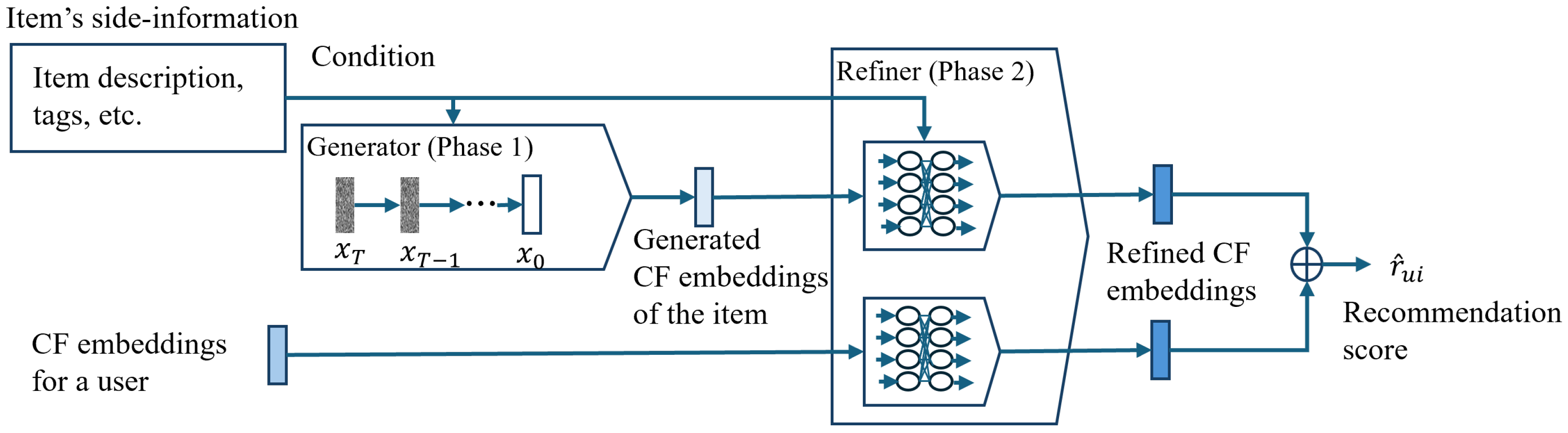
Figure 1 shows the two-phase recommendation of the proposed method. In the first phase, the DM-based generator generates collaborative embeddings of cold items using their side information as input. Then, the generated collaborative embeddings of cold items and the collaborative embeddings of users calculated by the base recommender are fed into the refiner to calculate more accurate recommendations for each user. The generated embeddings contain some errors that originated from information deficiency. For instance, coarse-grained side information of the cold items is given as the generation condition, and valuable user-side information, the ground-truth collaborative embeddings of users, is not considered. We employed the refiner to correct the error in the generated collaborative embeddings by the DM-based generator.
We train the DM-based generator first and then train the refiner using the trained generator. Although we adopted the refiner, it is worth noting that we can directly use the collaborative embeddings of cold items generated by the DM-based generator to calculate recommendation scores just by applying dot products with user collaborative embeddings.

3.2.2. DM-Based Generator

The DM-based generator is a DM that generates collaborative embeddings e i of cold items from their side information c i as its generation condition. Therefore, in the training, we assigned e i and c i to the original data x 0 and c in Algorithm 1, respectively.
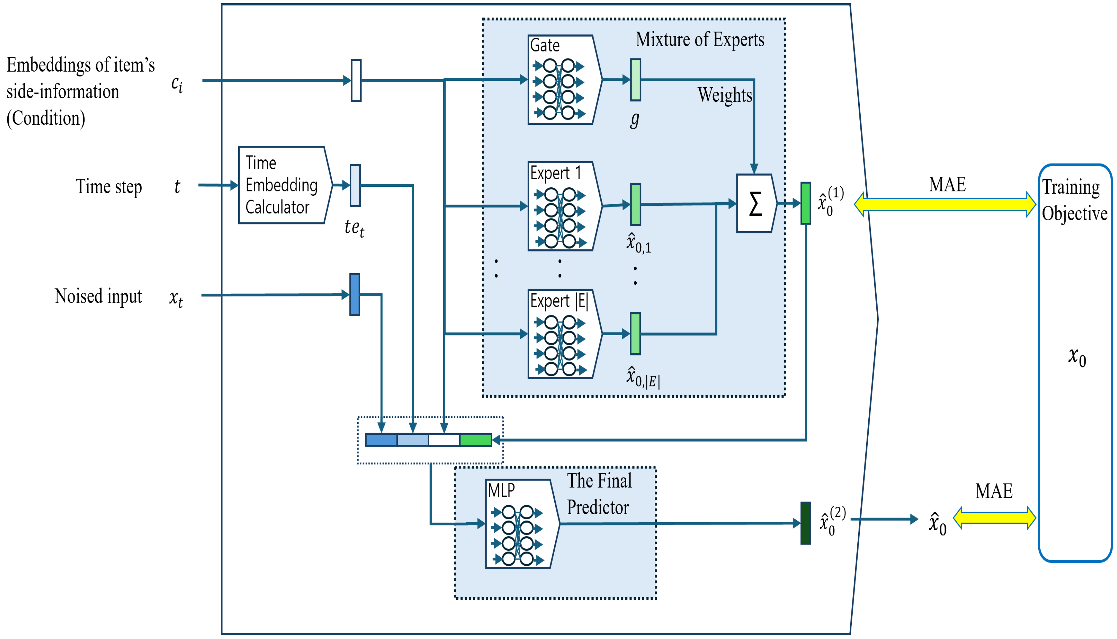
Network architecture: For the x 0 -predictor x ^ θ ( x t , t , c i ) in Equation (8), instead of simple MLPs used in previous works [33,38], we added a guideline predictor consisting of a Mixture-of-Experts network (MoE) [58] to handle complex collaborative embedding distributions more effectively and adapt to diverse patterns with limited information on items’ side information. As shown in Figure 2, side information c i is given to the MoE to generate the first prediction of collaborative embedding x ^ 0 ( 1 ) ; then, with the inputs of DM, x ^ 0 ( 1 ) is fed into the MLP as additional information to predict x 0 , the collaborative embedding of cold item e i .
The MoE network consists of the gate network represented in Equation (11) and multiple experts e E that have the same network structure described in Equation (12), but different parameters are learned from each other.
g = s i g m o i d ( W g × c i + b g )
where g R | E | indicates the gate vector whose elements represent the weights assigned to individual experts’ output. W g R | E | × d c o n d , b g R | E | , and s i g m o i d indicate the gate network’s weight matrix, bias, and the sigmoid activation function, respectively.
x ^ 0 , e = W e × c i + b e
where W e R d c f × d c o n d and b e R d c f represent the weight matrix and bias of individual expert e. We chose a single-layer linear transformation without an activation function as the expert network because our pre-experiments showed that the configuration mentioned above shows better performance than more complicated non-linear networks, which is also supported by other works [20,59].
The first prediction x ^ 0 ( 1 ) for x 0 is calculated by the weighted sum of the experts’ outputs, as represented in Equation (13).
x ^ 0 ( 1 ) = t a n h ( Σ e = 1 | E | g i · x ^ 0 , e )
where g i and t a n h represent the value of the i-th element of g and the hyperbolic tangent activation function, respectively.
With x ^ 0 ( 1 ) , x t , c i , and the time step embedding [60] t e t R d t i m e , which is related to time step t, are concatenated and passed to the three-layer MLP to calculate the final prediction x ^ 0 ( 2 ) for x 0 . The network structure of the MLP is represented in Equations (14)–(16).
m l p ( 1 ) = s w i s h ( W m l p ( 1 ) × ( x t x ^ 0 ( 1 ) c i t e t ) + b m l p ( 1 ) )
where W m l p ( 1 ) R d c f × ( 2 × d c f + d c o n d + d t i m e ) and b m l p ( 1 ) R d c f represent the weight matrix and bias of the first layer of the MLP. s w i s h indicates the swish activation function [61].
m l p ( 2 ) = s w i s h ( W m l p ( 2 ) × m l p ( 1 ) + b m l p ( 2 ) )
x ^ 0 ( 2 ) = W m l p ( 3 ) × m l p ( 2 ) + b m l p ( 3 )
where W m l p ( l ) R d c f × d c f and b m l p ( l ) R d c f represent the weight matrix and bias of the l-th layer of the MLP. The only difference in the network structure between the second and third layers is the existence of the activation function. We attached a linear transformation layer as the third layer because the value of collaborative embeddings does not indicate the probability, and we do not have concrete prior knowledge about its range.
Training: The quality of x ^ 0 ( 1 ) is important because the MLP that calculates the final prediction exploits the prediction of the MoE as its prediction guide. To improve the prediction accuracy of x ^ 0 ( 1 ) , we adopted the objective function in Equation (17) instead of Equation (10) in Algorithm 1.
L d = E t , x 0 , c ( x 0 x ^ 0 ( 1 ) 1 + x 0 x ^ 0 ( 2 ) 1 )
where · 1 indicates the L1-norm. Instead of MSE, we adopted MAE because the scale of the element of the embedding vector that we want to predict is small, and MAE forces the model to reduce small prediction errors. We give the fixed weight to each error in Equation (17) to keep the model simple because our pre-experiments achieved the best performance with the configuration.
Inference: We can generate the collaborative embedding of the cold item by calculating x 0 in Algorithm 2 with c i as the input condition c.

3.3. Second-Phase Refiner

The refiner’s purpose in the second phase is to reduce the error that may be caused by the lack of user-side information or coarse side information of cold items by adjusting the ground-truth user collaborative embeddings and the generated item collaborative embeddings to predict more accurate user–item interactions. Figure 3 shows the architecture of the refiner (Refiner). The ground-truth user collaborative embeddings e u , generated item collaborative embeddings e ^ i , and items’ side information c i are given. With the information provided, the Refiner calculates the recommendation score r ^ u i which is proportional to the probability of interaction between user u and item i by calculating Equation (18) with the refined user vector e ^ u + and item vector e ^ i + . The Refiner adopts two sub-networks: one for users and one for items. The user-side sub-network that calculates e ^ u + is represented in Equation (19).
r ^ u i = e ^ u + · e ^ i +
e ^ u + = W U ( 2 ) × B N ( t a n h ( W U ( 1 ) × e u + b U ( 1 ) ) ) + b U ( 2 )
where W U ( 1 ) , W U ( 2 ) R d c f × d c f , and b U ( 1 ) , b U ( 2 ) R d c f represent weights and biases of the first and second layer, respectively. B N indicates the batch normalization [62].
The item-side sub-network comprises the two layers represented in Equations (20) and (21).
h i = B N ( t a n h ( W I ( 1 ) × ( e ˜ i c i ) + b I ( 1 ) ) )
e ^ i + = W I ( 2 ) × ( h i e ˜ i c i ) + b I ( 2 )
where W I ( 1 ) R d c f × ( d c f + d c o n d ) and W I ( 2 ) R d c f × ( 2 d c f + d c o n d ) , and b I ( 1 ) , b I ( 2 ) R d c f represent weights and biases of the first and second layers, respectively. At the inference time, e ˜ i indicates the predicted collaborative embedding of the cold item calculated by the DM-based generator. We designed each of the two layers as a collaborative embedding refiner, which refines e ˜ i based on the side information c i and the output of the previous layer as guidelines.
Training: To train the Refiner, we use the interaction information R t r that is used to train the base recommender and the ground-truth item collaborative embeddings e i calculated by the base recommender. For each positive interaction of user u whose value of r u i R t r is one, five negative user–item interactions whose value of r u i R t r is zero are sampled. The sets of positive and negative interactions are joined to create the training dataset D t r . With D t r , the Refiner is trained to minimize the objective function represented in Equation (22). The details of the training procedure are found in Algorithm 3.
L R e f i n e r = 1 | D t r | Σ r u i D t r r u i r ^ u i 2 2
Algorithm 3 Refiner Train
Input: Dataset D t r , the sets of ground-truth user, item, generated item collaborative embeddings, and items’ side information: E U , E I , E ^ I , and C I
Output: Trained model parameter θ
1:
Initialize θ with random values
2:
while  θ is not converged do
3:
    Randomly sample a batch D t r D t r
4:
    for all  r u i D t r  do
5:
        Extract e u , e i , e ^ i , and c i from E U , E I , E ^ I , and C I , respectively
6:
        Calculate e ^ u + and e ^ i + by using Equations (19)–(21).
7:
        Calculate r ^ u i by using Equation (18) with e ^ u + and e ^ i +
8:
        Calculate loss L R e f i n e r by using Equation (22)
9:
        Update θ using gradient descent with θ L R e f i n e r
10:
    end for
11:
end while
When we calculate e ^ i + , following the ideas of Wang et al. [20] and Volkovs et al. [19], input e ˜ i for the item-side sub-network represented in Equations (20) and (21) is sampled by Equation (23). By allowing the network access to the ground-truth and generated embeddings alternately for the given side information, we expect the model to more accurately guess the ground-truth embeddings based on the generated embedding under the given side information.
e ˜ i = e ^ i , with probability 0.5 e i , otherwise
Inference: The Refiner calculates refined user embeddings e ^ u + from users’ ground-truth collaborative embeddings. Similarly, refined item embeddings e ^ i + are calculated with the generated collaborative embeddings and side information of cold items as input. Once calculated, we can store the two kinds of embeddings in the system. For an arbitrary user u and cold item i pair, we can calculate r ^ u i by using Equation (18) with e ^ u + and e ^ i + . The ordered recommendation list of k-items for user u, L u k , is calculated by sorting the top k items that have the highest r ^ u i scores in descending order.

4. Evaluation Environment

We describe the evaluation environment, which includes the datasets used, evaluation metrics, and the baseline methods compared in the evaluation.

4.1. Datasets

We evaluated the proposed method with two real-world datasets, CiteULike and MovieLens25M.
CiteULike [63] is a well-known dataset used for research in recommender systems. The data were collected from CiteULike, an online reference management and social bookmarking platform where users can save and share academic papers. The dataset includes about 0.2 million user–save–article interactions. As side information, abstracts of the articles are provided. We followed [19,20,63] to calculate the embeddings for side information. Specifically, we first selected the top 8000 high-scored words from the words that appeared in the abstract corpus by applying tf-idf and constructed an 8000-dimensional multi-hot feature vector for each paper. After that, the multi-hot vectors were deduced to 300-dimensional embedding vectors by applying SVD [64]. We randomly selected 1018 and 2378 non-interacted items as the validation and test item sets, and interactions related to the two item sets were used as validation and test sets, respectively. The remainder of the interactions were used as the training set.
MovieLens25M (ML25M) [65] is a dataset for movie recommendation research, released by the Grouplens (https://grouplens.org/ (accessed on 30 March 2025)). It contains 25 million user ratings and movie metadata and is one of the largest publicly available datasets. The dataset includes side information such as titles, genres, release years, and additional tagging information. We calculated the 400-dimensional side information embedding from the tag genome data [66] of each movie by applying VAE [52]. For train–validation–test data separation, we made five non-intersected movie groups of the same size. We selected one group and used 70% of its movies as the test movie set and the remaining 30% as the validation movie set. The last four movie groups were used as the train movie set. The interaction data associated with the three movie sets were used as the test, validation, and training sets. From all sets, ratings of less than 3.0 in 5-scale ratings were filtered out as negative ratings. We performed 5-fold cross-validation by selecting another group for the test and validation groups.
Collaborative embedding of base CF method: We used BPR [67], one of the most popular CF algorithms in academia and industry, as the base CF method to compute the collaborative embeddings. We calculated the collaborative embeddings of dimensions 200 and 128 using the training dataset for CiteULike and ML25M, respectively. Table 2 represents the statistics of the datasets.
Quality of side information embeddings: We used SVD and VAE to obtain compact embeddings for words and tag distributions, respectively. Both methods are optimized to minimize the reconstruction error of the original word or tag distribution of an item from the embedding. To investigate whether severe compression could result in information loss, we conducted experiments by varying the embedding dimensions. We observed that increasing the dimensionality beyond the values reported in the description of CiteULike and ML25M did not lead to significant improvements in reconstruction performance. This suggests that the chosen dimensions are reasonable balances between compression and information preservation.

4.2. Evaluation Metrics

We assessed the recommendation performance by employing Precision@k (P@k) [68], Recall@k (R@k) [68], and NDCG@k (N@k) [69].
P@k represents the fraction of relevant items (the items that the user has interacted with) included in the top k positions of the recommendation list. It is computed using Equation (24).
P @ k = 1 | U | u U | L u k I u + | | L u k |
R@k measures the proportion of the interacted items within the top k recommendations relative to the total number of interacted items in the test dataset. It is determined by Equation (25).
R @ k = 1 | U | u U | L u k I u + | | I u + |
Here, I u + refers to the set of items that user u has interacted with, while L u k denotes the set of recommended items that appeared within the top k positions of the recommendation list for u.
N@k considers the interacted items’ relevance and ranking position within the top k recommendations. Even if the number of relevant items in the top-k list remains the same, N@k assigns higher scores to items appearing in earlier ranks. It is computed using Equation (26).
N @ k = D C G @ k I D C G @ k
D C G @ k = 1 | U | u U l = 1 k 1 I u + ( l ) m a x ( 1 , l o g 2 ( l ) )
Here, 1 I u + ( l ) in Equation (27) represents the indicator function that identifies whether an item appeared in the l-th position in L u k is included in I u + or not. It takes a value of one if the item is included in I u + , and zero otherwise. I D C G @ k (Ideal D C G @ k ) corresponds to the maximum possible D C G @ k where all relevant items ( i I u + ) are ranked consecutively from the top of the recommendation list.

4.3. Comparison Methods

We conducted a comparison between the proposed method and five existing related approaches.
DropoutNet [19]: This approach is designed to predict recommendation scores obtained from the base recommender model by randomly masking collaborative embeddings in its input pair’s CF embedding and side information embedding during training. By doing so, the model is trained to infer missing collaborative embeddings based solely on the item’s side information, enabling it to generalize to cold items more effectively.
Heater [20]: Heater aims to directly predict collaborative embeddings by optimizing an objective function that enforces the model to learn collaborative embeddings from cold items’ side information. The recommendation score is then derived from the predicted collaborative embeddings. To enhance prediction accuracy, Heater employs a Mixture-of-Experts predictor and CF embedding dropout strategies.
CVAR [15]: This method utilizes two encoders and a decoder within a variational autoencoder (VAE) framework [52] to transform the item’s side information into collaborative embeddings. The first encoder processes pre-trained collaborative embeddings from a base CF model while the decoder reconstructs the collaborative embeddings from the encoded representations. Meanwhile, the second encoder learns representations from the item’s side information. The objective function encourages the encoding from the second encoder to closely match that of the first encoder for the same item, ensuring that the decoder can generate valid collaborative embeddings, thus improving cold item recommendations.
CCFC [22]: CCFC leverages contrastive learning to enhance CF embedding prediction. This method enforces similar items (e.g., those with overlapping user interaction histories) to have closely aligned collaborative embeddings while ensuring that the learned embeddings remain distinct from those of unrelated items. Through this contrastive learning strategy, CCFC refines the quality of side information-driven CF embedding predictions.
GME [53]: It enhances the cold item’s side information representation by aggregating information from its neighbors with similar side information using a graph attention network. The score predictor then leverages these enriched side information representations to estimate recommendation scores effectively.
DMCIR: DMCIR (Diffusion Model-based Cold Item Recommender) indicates the DM-based generator of the proposed method to generate the collaborative embeddings from cold items’ side information. Since it generates the collaborative embeddings of the item side, it can recommend items to users by calculating dot product between the generated collaborative embeddings of candidate items and the collaborative embeddings of target users.
DMCIR+: DMCIR+ represents the results that applied the Refiner of the proposed method to the collaborative embeddings generated by DMCIR.
The methods were implemented and evaluated using TensorFlow 2.15 (https://www.tensorflow.org/ (accessed on 30 March 2025)) on a machine equipped with a Ryzen Threadripper Pro 3945WX 12-core CPU (AMD), 128 GB of RAM (Samsung, Suwon Republic of Korea), and a TITAN RTX GPU (nVidia, Santa Clara, CA, USA). The source code for the proposed method is publicly available at https://github.com/JungkyuHan/DMCIR (accessed on 30 March 2025). For the implementation of comparison methods, when the official source codes were available [15,19,20,22], we referred to them. Additionally, we adopted the hyperparameter settings that yielded the best validation performance. We evaluated the models with different initial model parameters five times and reported the average performance. DMCIR/DMCIR+ used the hyperparameters shown in Table 3.

5. Result Analysis

We conducted the experiments to address the following three research questions:
  • RQ1. How well does the diffusion model perform in cold item recommendations? How much can its performance be improved by incorporating the post-recommender model (the Refiner)?
  • RQ2. What are the optimal hyperparameter values for the DM-based generator in collaborative embedding prediction?
  • RQ3. To what extent does the quality of embeddings influence model performance?

5.1. Overall Performance (RQ1)

Table 4 shows the overall performance. DMCIR, the recommendation that directly used the collaborative embeddings generated by the DM-based generator, shows decent performance. Only Heater in ML25M and CCFC in CiteULike outperform or match DMCIR. The observation highlights the diffusion model’s superior capability in generating high-quality outputs. DMCIR+, recommended with the Refiner-generated collaborative embeddings from DMCIR’s results, achieved the best performance among all other comparison methods over all datasets. This observation suggests that certain collaborative information is challenging to infer solely from the items’ side information and that some can be effectively captured through a refinement process incorporating user-side collaborative embeddings.
Among the comparison methods, those that incorporate explicit collaborative embedding training guidance into their objective functions—namely Heater and CCFC—consistently outperform the others in most cases. This observation indicates that providing predictive guidance on collaborative embeddings during training effectively enhances the performance of cold item recommendation. DMCIR+ leverages the output of DMCIR as prediction guidance and achieves the best performance.
The elapsed time for cold item recommendation is shown in Table 5. It demonstrates how quickly the system can incorporate new items into the top recommendations for relevant users. “Item Gen” refers to the time required by the DM-based generator to generate item embeddings. “Item Refine” and “User Refine” indicate the time taken by the Refiner to refine item and user embeddings, respectively. As shown, generating about 17,000 item embeddings takes approximately 40 seconds, and the Refiner completes both refinement steps in less than one second. The calculation of recommendation item lists (“Rec” column) for ML25M (162,540 users and 13,816 candidate items) is also completed in under one second. Since the generation and refinement steps are performed only once per item, the “Rec” process dominates the actual recommendation cost. We argue that achieving recommendations for approximately 160,000 users in under one second is fast enough for deployment in commercial recommender systems.

5.2. DM’s Hyperparameter Effect (RQ2)

DM’s Noise Schedule: Here, we evaluate the performance of DMCIR with various values of β e in Equation (2). Figure 4 plots the decay ratio of x 0 in the forward process to timestep t ( α t ¯ in Equation (3)) for different β e values. As the value of β e increases, the speed of the original signal decay also increases. Table 6 plots the performance of DMCIR with β e { 0.02 , 0.03 , 0.04 , 0.05 , 0.06 } . The other hyperparameters, the number of experts | E | and the maximum timestep T are fixed to 5 and 400, respectively. The average performance increases as β e increases to 0.05. The performance starts to decrease at β e = 0.06 .
This trend indicates that the original information available in the last part of the forward process affects the reconstruction accuracy. As shown β e = 0.02 in Figure 4, when β e is small, the signal-to-noise ratio (SNR) of the original information does not become zero at T. As Lin et al. [70] pointed out, the remaining original information in the training phase makes the denoiser (predictor) try to seek the original information at x T , which is regarded as a pure Gaussian noise. Because we do not know collaborative embeddings of cold items, we set a pure Gaussian noise as x T is in the inference phase. The performance drop at small β e = 0.02 is caused because the denoiser considers a noise as information from x 0 . The phenomenon is mitigated as β e increases, but when β e is greater than 0.05, the available information of x 0 in the last part of the forward process becomes too small. That also hinders the performance of the denoiser.
It is important to determine the optimal value of β e . Based on our experimental result showing that β e [ 0.04 , 0.05 ] yields consistently fair performance across datasets, we suggest 0.04 to 0.05 as a reasonable choice.
Maximum Timesteps: For DM, an optimal value of the maximum timesteps T is critical. When the value of T is too small, although the training and inference costs are reduced, the noise scale applied to each timestep increases. That makes the denoising process difficult. On the other hand, when the value of T is too large, the denoising process becomes easier, resulting in increased computational costs. Figure 5 shows DMCIR’s performance with the CiteULike ((a)) and ML25M ((b)) datasets to various T { 100 , 200 , 300 , 400 , 500 , 600 } . We fixed the other parameters as β e = 0.05 and | E | = 5 .
Generally, the recommendation performance increases as the value of T increases and reaches its peak at 300 and 400. After that, the performance starts to decline. This observation is caused by the extremely small noise size of the single timestep. The extremely small size of the noise is also difficult to predict accurately. Considering the performance and cost trade-off, the value of T as 300 or 400 is a good choice.
The Number of Experts in x 0 -Predictor of DM: The x 0 -predictor of DMCIR adopts a Mixture-Of-Experts architecture to generate the first prediction x ^ 0 ( 1 ) in Equation (13), which is used for prediction guidance of DM. In Figure 6, we show the recommendation performance of DMCIR with CiteULike ((a)) and ML25M ((b)) datasets to various number of experts | E | { 0 , 1 , 3 , 5 , 7 } . “ | E | = 0 ” indicates that MoE in Figure 2 is removed. The other parameters were fixed as β e = 0.05 and T = 400 .
In all datasets, the worst performance was observed when “ | E | = 0 ”, indicating that MoE contributes to the recommendation performance. The performance increases as | E | increases to some point, | E | = 3 for CiteULike and | E | = 5 for ML25M, and then starts to decline in both datasets but the details are different. The performance gain caused by the MoE with the CiteULike dataset is smaller than that with ML25M, which shows significant improvement. The observation was caused by the characteristics of the datasets. The users and side information of items in the CiteULike dataset are specialists and abstracts of papers. In contrast, the users and side information of items in the ML25M dataset are ordinary people and tags assigned to movies. Therefore, the uncertainty in the relationship between user interactions and side information is lower in the CiteULike dataset, which allows the performance of the x 0 -predictor without MoE to approach that of the MoE-enhanced x 0 -predictor.

5.3. Embedding Quality (RQ3)

Generated embedding quality to the Refiner’s performance: The Refiner takes the collaborative embeddings calculated by DM-based generator to calculate refined collaborative embeddings for the final recommendation. Therefore, the relationship analysis between input and the final recommendation quality is important. To this end, we compared the performance of the DMCIR model with two different configurations and the performance of the two DMCIR+ models whose input collaborative embeddings are the output of each DMCIR model. Table 7 shows the result. DMCIR 0 and DMCIR o p t indicate that DMCIR with the number of experts is zero and with the best number of experts (three for CiteULike, five for ML25M), respectively. DMCIR 0 + and DMCIR o p t + use the outputs of DMCIR 0 and DMCIR o p t as inputs, respectively.
The performance of DMCIR+ is proportional to its input item collaborative embeddings. This indicates that the qualitative first prediction of item collaborative embeddings is essential to calculate more accurate refined embeddings. An interesting finding is that while the performance difference between DMCIR 0 and DMCIR o p t and the difference between DMCIR 0 + and DMCIR o p t + in CiteULike are similar, in ML25M the difference between DMCIR 0 + and DMCIR o p t + is much smaller compared to the difference between DMCIR 0 and DMCIR o p t . That indicates that, in the ML25M dataset, some information captured by the MoE architecture in DMCIR from item collaborative embeddings can be compensated by the refining process, which is re-considering user embeddings and user–item interactions. Thus, further research is required to extract and integrate information using integrated architecture. However, calculating high-quality collaborative embeddings upstream is still important to achieving top recommendation accuracy, especially at the top part of the recommendation list that users most frequently examine.
Side information quality to model performance: Since the proposed method relies on side information as a pivotal input, the quality of the side information is crucial. To investigate the relationship between the quality of side information and model performance, we evaluated our method using side information embeddings of varying quality. Specifically, we calculated degraded side information by randomly dropping p % of the original content prior to embedding calculation. Figure 7 shows the relative R@20 scores calculated with side information of different qualities. Across all datasets and model types, performance consistently degrades with lower-quality side information, demonstrating that side information quality is a critical factor in the effectiveness of the proposed method.
Embedding Transformation Analysis: Here, we analyze how the Refiner transforms its input collaborative embeddings—specifically, the ground-truth user embeddings and the generated item embeddings. Since the Refiner projects these inputs into a different space, it is not straightforward to directly compare the input and output embeddings of the Refiner. To address this, we evaluate the transformation by examining the relative angles between embeddings. We compute the pairwise cosine similarity and construct similarity matrices for each set of vectors. For each dataset, we obtain four matrices: S U i n , S I i n , S U r e , S I r e , representing the similarity matrices for users’ ground-truth embeddings, items’ generated embeddings, refined user embeddings, and refined item embeddings, respectively.
Figure 8 shows the value distribution of the elements in the absolute difference matrix D x = | S x i n S x r e | . Across datasets, the relative angles between user embeddings remain mostly unchanged. However, for item embeddings, the CiteULike dataset shows only minor changes, whereas the ML25M dataset exhibits more significant transformations. This observation is further illustrated in Figure 9, which displays side-by-side visualizations of item embeddings before and after refinement. The visualized distributions of embeddings in CiteULike are similar to each other, whereas in ML25M, they show more noticeable differences. We think that this difference is caused by the varying quality of side information. Compared to the abstracts of academic papers used in CiteULike, the tags associated with full-length movies in ML25M are less effective in representing item content. As a result, Refiner performs more substantial transformations on the embeddings generated from the less informative movie tags.

6. Conclusions

This paper presented a novel diffusion model framework as an add-on solution for improving cold item recommendation performance in collaborative filtering (CF) systems. Our diffusion model-based generator generates collaborative embeddings for cold items by effectively leveraging items’ side information. The second-phase refiner further enhances recommendation accuracy by utilizing simple neural network components and dropout regularization, ensuring effective refinement of embeddings with minimal system overhead.
Through extensive experiments on real-world datasets, we demonstrated that our approach outperforms state-of-the-art methods in cold item scenarios, particularly at the start of item introduction. The model’s performance and insights from hyperparameter sensitivity and ablation studies highlight the practical value and flexibility of integrating diffusion models into recommender systems. Our findings suggest that the diffusion models are a promising direction for addressing long-standing challenges in cold item recommendation.
Future work will explore four main directions: (1) Developing more effective predictor architectures for the diffusion model to enhance the accuracy of generated collaborative embeddings. (2) Designing an end-to-end architecture that tightly integrates the diffusion generation module and the refiner module to improve overall efficiency and performance. (3) Conducting a thorough study for a more comprehensive analysis of the noise scheduler’s stability in the diffusion model in the context of cold item recommendations. (4) Investigating structured comparison techniques to improve the reliability of item representations in cold-start recommendation settings.

Author Contributions

Conceptualization, J.H.; methodology, J.H. and S.C.; software, J.H.; validation, J.H. and S.C.; data curation, J.H. and S.C.; writing—original draft preparation, J.H.; writing—review and editing, J.H. and S.C. All authors have read and agreed to the published version of the manuscript.

Funding

This work was supported by the Dong-A University research fund.

Institutional Review Board Statement

Not applicable.

Informed Consent Statement

Not applicable.

Data Availability Statement

Publicly available datasets were analyzed in this study. This data can be found here: https://github.com/JungkyuHan/DMCIR (accessed on 30 March 2025).

Acknowledgments

This work was supported by the Dong-A University research fund.

Conflicts of Interest

The authors declare no conflicts of interest.

Abbreviations

The following abbreviations are used in this manuscript:
CFCollaborative Filter
DMDiffusion Model

References

  1. Su, X.; Khoshgoftaar, T.M. A Survey of Collaborative Filtering Techniques. Adv. Artif. Intell. 2009, 2009. [Google Scholar] [CrossRef]
  2. Lam, X.N.; Vu, T.; Le, T.D.; Duong, A.D. Addressing cold-start problem in recommendation systems. In Proceedings of the 2nd International Conference on Ubiquitous Information Management and Communication, Suwon, Republic of Korea, 31 January–1 February 2008; pp. 208–211. [Google Scholar] [CrossRef]
  3. Adomavicius, G.; Tuzhilin, A. Toward the next generation of recommender systems: A survey of the state-of-the-art and possible extensions. IEEE Trans. Knowl. Data Eng. 2005, 17, 734–749. [Google Scholar] [CrossRef]
  4. Yu, K.; Schwaighofer, A.; Tresp, V.; Xu, X.; Kriegel, H.P. Probabilistic memory-based collaborative filtering. IEEE Trans. Knowl. Data Eng. 2004, 16, 56–69. [Google Scholar] [CrossRef]
  5. Fallah, A.; Mokhtari, A.; Ozdaglar, A. Generalization of Model-Agnostic Meta-Learning Algorithms: Recurring and Unseen Tasks. In Proceedings of the Advances in Neural Information Processing Systems, Virtual, 6–14 December 2021; Volume 34, pp. 5469–5480. [Google Scholar]
  6. Finn, C.; Abbeel, P.; Levine, S. Model-Agnostic Meta-Learning for Fast Adaptation of Deep Networks. In Proceedings of the 34th International Conference on Machine Learning—Volume 70, Sydney, Australia, 6–11 August 2017; JMLR.org, ICML’17. pp. 1126–1135. [Google Scholar]
  7. Lee, H.; Im, J.; Jang, S.; Cho, H.; Chung, S. MeLU: Meta-Learned User Preference Estimator for Cold-Start Recommendation. In Proceedings of the 25th ACM SIGKDD International Conference on Knowledge Discovery & Data Mining, Anchorage, AK, USA, 4–8 August 2019; KDD’19; pp. 1073–1082. [Google Scholar] [CrossRef]
  8. Dong, M.; Yuan, F.; Yao, L.; Xu, X.; Zhu, L. MAMO: Memory-Augmented Meta-Optimization for Cold-Start Recommendation. In Proceedings of the 26th ACM SIGKDD International Conference on Knowledge Discovery & Data Mining, Virtual, 23–27 August 2020; KDD’20. pp. 688–697. [Google Scholar] [CrossRef]
  9. Lin, X.; Wu, J.; Zhou, C.; Pan, S.; Cao, Y.; Wang, B. Task-Adaptive Neural Process for User Cold-Start Recommendation. In Proceedings of the Web Conference 2021, Virtual, 19–23 April 2021; WWW’21. pp. 1306–1316. [Google Scholar] [CrossRef]
  10. Pan, F.; Li, S.; Ao, X.; Tang, P.; He, Q. Warm Up Cold-Start Advertisements: Improving CTR Predictions via Learning to Learn ID Embeddings. In Proceedings of the 42nd International ACM SIGIR Conference on Research and Development in Information Retrieval, Paris, France, 21–25 July 2019; SIGIR’19. pp. 695–704. [Google Scholar] [CrossRef]
  11. Lu, Y.; Fang, Y.; Shi, C. Meta-Learning on Heterogeneous Information Networks for Cold-Start Recommendation. In Proceedings of the 26th ACM SIGKDD International Conference on Knowledge Discovery & Data Mining, Virtual, 23–27 August 2020; KDD’20. pp. 1563–1573. [Google Scholar] [CrossRef]
  12. Zhu, Y.; Xie, R.; Zhuang, F.; Ge, K.; Sun, Y.; Zhang, X.; Lin, L.; Cao, J. Learning to Warm Up Cold Item Embeddings for Cold-Start Recommendation with Meta Scaling and Shifting Networks. In Proceedings of the 44th International ACM SIGIR Conference on Research and Development in Information Retrieval, Virtual, 11–15 July 2021; SIGIR’21. pp. 1167–1176. [Google Scholar] [CrossRef]
  13. Salha-Galvan, G.; Hennequin, R.; Chapus, B.; Tran, V.A.; Vazirgiannis, M. Cold Start Similar Artists Ranking with Gravity-Inspired Graph Autoencoders. In Proceedings of the 15th ACM Conference on Recommender Systems, Amsterdam, The Netherlands, 27 September–1 October 2021; RecSys’21. pp. 443–452. [Google Scholar] [CrossRef]
  14. Li, J.; Jing, M.; Lu, K.; Zhu, L.; Yang, Y.; Huang, Z. From Zero-Shot Learning to Cold-Start Recommendation. In Proceedings of the Thirty-Third AAAI Conference on Artificial Intelligence, Honolulu, HI, USA, 27 January–1 February 2019. AAAI’19. [Google Scholar] [CrossRef]
  15. Zhao, X.; Ren, Y.; Du, Y.; Zhang, S.; Wang, N. Improving Item Cold-Start Recommendation via Model-Agnostic Conditional Variational Autoencoder. In Proceedings of the 45th International ACM SIGIR Conference on Research and Development in Information Retrieval, Madrid, Spain, 11–15 July 2022; SIGIR’22. pp. 2595–2600. [Google Scholar] [CrossRef]
  16. Hansen, C.; Hansen, C.; Simonsen, J.G.; Alstrup, S.; Lioma, C. Content-Aware Neural Hashing for Cold-Start Recommendation. In Proceedings of the 43rd International ACM SIGIR Conference on Research and Development in Information Retrieval, Virtual, 25–30 July 2020; SIGIR’20. pp. 971–980. [Google Scholar] [CrossRef]
  17. Oramas, S.; Nieto, O.; Sordo, M.; Serra, X. A Deep Multimodal Approach for Cold-Start Music Recommendation. In Proceedings of the 2nd Workshop on Deep Learning for Recommender Systems, Como, Italy, 27 August 2017; DLRS 2017. pp. 32–37. [Google Scholar] [CrossRef]
  18. Raziperchikolaei, R.; Liang, G.; Chung, Y.j. Shared Neural Item Representations for Completely Cold Start Problem. In Proceedings of the 15th ACM Conference on Recommender Systems, Amsterdam, The Netherlands, 27 September–1 October 2021; RecSys’21. pp. 422–431. [Google Scholar] [CrossRef]
  19. Volkovs, M.; Yu, G.; Poutanen, T. DropoutNet: Addressing Cold Start in Recommender Systems. In Proceedings of the Advances in Neural Information Processing Systems, Long Beach, CA, USA, 4–9 December 2017; Volume 30. [Google Scholar]
  20. Zhu, Z.; Sefati, S.; Saadatpanah, P.; Caverlee, J. Recommendation for New Users and New Items via Randomized Training and Mixture-of-Experts Transformation. In Proceedings of the 43rd International ACM SIGIR Conference on Research and Development in Information Retrieval, Virtual, 25–30 July 2020; pp. 1121–1130. [Google Scholar] [CrossRef]
  21. Wei, Y.; Wang, X.; Li, Q.; Nie, L.; Li, Y.; Li, X.; Chua, T.S. Contrastive Learning for Cold-Start Recommendation. In Proceedings of the 29th ACM International Conference on Multimedia, Chengdu, China, 20–24 October 2021; MM’21. pp. 5382–5390. [Google Scholar] [CrossRef]
  22. Zhou, Z.; Zhang, L.; Yang, N. Contrastive Collaborative Filtering for Cold-Start Item Recommendation. In Proceedings of the ACM Web Conference 2023, Austin, TX, USA, 30 April–4 May 2023; WWW’23. pp. 928–937. [Google Scholar] [CrossRef]
  23. Pazzani, M.J.; Billsus, D. Content-Based Recommendation Systems. In The Adaptive Web: Methods and Strategies of Web Personalization; Springer: New York, NY, USA, 2007; pp. 325–341. [Google Scholar] [CrossRef]
  24. Bazzi, A.; Slock, D.T.M.; Meilhac, L. A Newton-type Forward Backward Greedy method for multi-snapshot compressed sensing. In Proceedings of the 2017 51st Asilomar Conference on Signals, Systems, and Computers, Pacific Grove, CA, USA, 29 October–1 November 2017; pp. 1178–1182. [Google Scholar] [CrossRef]
  25. Kakiashvili, T.; Koczkodaj, W.W.; Woodbury-Smith, M. Improving the medical scale predictability by the pairwise comparisons method: Evidence from a clinical data study. Comput. Methods Programs Biomed. 2012, 105, 210–216. [Google Scholar] [CrossRef] [PubMed]
  26. Sohl-Dickstein, J.; Weiss, E.A.; Maheswaranathan, N.; Ganguli, S. Deep unsupervised learning using nonequilibrium thermodynamics. In Proceedings of the 32nd International Conference on International Conference on Machine Learning—Volume 37, Lille, France, 6–11 July 2015; ICML’15. pp. 2256–2265. [Google Scholar]
  27. Ho, J.; Jain, A.; Abbeel, P. Denoising diffusion probabilistic models. In Proceedings of the 34th International Conference on Neural Information Processing Systems, Virtual, 6–12 December 2020. NIPS’20. [Google Scholar]
  28. Ramesh, A.; Pavlov, M.; Goh, G.; Gray, S.; Voss, C.; Radford, A.; Chen, M.; Sutskever, I. Zero-Shot Text-to-Image Generation. In Proceedings of the 38th International Conference on Machine Learning, Virtual, 18–24 July 2021; Volume 139, pp. 8821–8831. [Google Scholar]
  29. Croitoru, F.A.; Hondru, V.; Ionescu, R.T.; Shah, M. Diffusion Models in Vision: A Survey. IEEE Trans. Pattern Anal. Mach. Intell. 2023, 45, 10850–10869. [Google Scholar] [CrossRef] [PubMed]
  30. Lovelace, J.; Kishore, V.; Wan, C.; Shekhtman, E.; Weinberger, K.Q. Latent diffusion for language generation. In Proceedings of the 37th International Conference on Neural Information Processing Systems, New Orleans, LA, USA, 10–16 December 2023. NIPS’23. [Google Scholar]
  31. He, H.; Zhang, J.; Chen, H.; Chen, X.; Li, Z.; Chen, X.; Wang, Y.; Wang, C.; Xie, L. A diffusion-based framework for multi-class anomaly detection. In Proceedings of the Thirty-Eighth AAAI Conference on Artificial Intelligence and Thirty-Sixth Conference on Innovative Applications of Artificial Intelligence and Fourteenth Symposium on Educational Advances in Artificial Intelligence, Vancouver, BC, Canada, 20–27 February 2024; AAAI Press: Washington, DC, USA, 2024. AAAI’24/IAAI’24/EAAI’24. [Google Scholar] [CrossRef]
  32. Huang, L.; Zhang, H.; Xu, T.; Wong, K.C. MDM: Molecular diffusion model for 3D molecule generation. In Proceedings of the Thirty-Seventh AAAI Conference on Artificial Intelligence and Thirty-Fifth Conference on Innovative Applications of Artificial Intelligence and Thirteenth Symposium on Educational Advances in Artificial Intelligence, Washington, DC, USA, 7–14 February 2023. AAAI’23/IAAI’23/EAAI’23. [Google Scholar] [CrossRef]
  33. Wang, W.; Xu, Y.; Feng, F.; Lin, X.; He, X.; Chua, T.S. Diffusion Recommender Model. In Proceedings of the 46th International ACM SIGIR Conference on Research and Development in Information Retrieval, Taipei, Taiwan, 23–27 July 2023; SIGIR’23. pp. 832–841. [Google Scholar] [CrossRef]
  34. Zhu, Y.; Wang, C.; Zhang, Q.; Xiong, H. Graph Signal Diffusion Model for Collaborative Filtering. In Proceedings of the 47th International ACM SIGIR Conference on Research and Development in Information Retrieval, Washington, DC, USA, 14–18 July 2024; SIGIR’24. pp. 1380–1390. [Google Scholar] [CrossRef]
  35. Hou, Y.; Park, J.D.; Shin, W.Y. Collaborative Filtering Based on Diffusion Models: Unveiling the Potential of High-Order Connectivity. In Proceedings of the 47th International ACM SIGIR Conference on Research and Development in Information Retrieval, Washington, DC, USA, 14–18 July 2024; SIGIR’24. pp. 1360–1369. [Google Scholar] [CrossRef]
  36. Walker, J.; Zhong, T.; Zhang, F.; Gao, Q.; Zhou, F. Recommendation via Collaborative Diffusion Generative Model. In Proceedings of the Knowledge Science, Engineering and Management, Singapore, 6–8 August 2022; pp. 593–605. [Google Scholar]
  37. Choi, J.; Hong, S.; Park, N.; Cho, S.B. Blurring-Sharpening Process Models for Collaborative Filtering. In Proceedings of the 46th International ACM SIGIR Conference on Research and Development in Information Retrieval, Taipei, Taiwan, 23–27 July 2023; SIGIR’23. pp. 1096–1106. [Google Scholar] [CrossRef]
  38. Zhao, J.; Wenjie, W.; Xu, Y.; Sun, T.; Feng, F.; Chua, T.S. Denoising Diffusion Recommender Model. In Proceedings of the 47th International ACM SIGIR Conference on Research and Development in Information Retrieval, Washington, DC, USA, 14–18 July 2024; SIGIR’24. pp. 1370–1379. [Google Scholar] [CrossRef]
  39. Ma, H.; Yang, Y.; Meng, L.; Xie, R.; Meng, X. Multimodal Conditioned Diffusion Model for Recommendation. In Proceedings of the Companion Proceedings of the ACM Web Conference 2024, Singapore, 13–17 May 2024; WWW’24. pp. 1733–1740. [Google Scholar] [CrossRef]
  40. Jiang, Y.; Xia, L.; Wei, W.; Luo, D.; Lin, K.; Huang, C. DiffMM: Multi-Modal Diffusion Model for Recommendation. In Proceedings of the 32nd ACM International Conference on Multimedia, Melbourne, Australia, 28 October–1 November 2024; MM’24. pp. 7591–7599. [Google Scholar] [CrossRef]
  41. Ma, H.; Xie, R.; Meng, L.; Chen, X.; Zhang, X.; Lin, L.; Kang, Z. Plug-in diffusion model for sequential recommendation. In Proceedings of the Thirty-Eighth AAAI Conference on Artificial Intelligence and Thirty-Sixth Conference on Innovative Applications of Artificial Intelligence and Fourteenth Symposium on Educational Advances in Artificial Intelligence, Vancouver, BC, Canada, 20–27 February 2024. AAAI’24/IAAI’24/EAAI’24. [Google Scholar] [CrossRef]
  42. Yang, Z.; Wu, J.; Wang, Z.; Yuan, Y.; Wang, X.; He, X. Generate what you prefer: Reshaping sequential recommendation via guided diffusion. In Proceedings of the 37th International Conference on Neural Information Processing Systems, New Orleans, LA, USA, 10–16 December 2023. NIPS’23. [Google Scholar]
  43. Niu, Y.; Xing, X.; Jia, Z.; Liu, R.; Xin, M.; Cui, J. Diffusion Recommendation with Implicit Sequence Influence. In Proceedings of the Companion Proceedings of the ACM Web Conference 2024, Singapore, 13–17 May 2024; WWW’24. pp. 1719–1725. [Google Scholar] [CrossRef]
  44. Wang, Y.; Liu, Z.; Wang, Y.; Zhao, X.; Chen, B.; Guo, H.; Tang, R. Diff-MSR: A Diffusion Model Enhanced Paradigm for Cold-Start Multi-Scenario Recommendation. In Proceedings of the 17th ACM International Conference on Web Search and Data Mining, Mérida, Mexico, 4–8 March 2024; WSDM’24. pp. 779–787. [Google Scholar] [CrossRef]
  45. Wei, T.R.; Fang, Y. Diffusion Models in Recommendation Systems: A Survey. arXiv 2025. [Google Scholar] [CrossRef]
  46. Luo, C. Understanding Diffusion Models: A Unified Perspective. arXiv 2022, arXiv:2208.11970. [Google Scholar]
  47. Pan, X.; Chen, Y.; Tian, C.; Lin, Z.; Wang, J.; Hu, H.; Zhao, W.X. Multimodal Meta-Learning for Cold-Start Sequential Recommendation. In Proceedings of the 31st ACM International Conference on Information & Knowledge Management, Atlanta, GA, USA, 17–21 October 2022; CIKM’22. pp. 3421–3430. [Google Scholar] [CrossRef]
  48. Sun, Y.; Han, J. Mining Heterogeneous Information Networks: A Structural Analysis Approach. SIGKDD Explor. Newsl. 2013, 14, 20–28. [Google Scholar] [CrossRef]
  49. Fu, T.y.; Lee, W.C.; Lei, Z. HIN2Vec: Explore Meta-Paths in Heterogeneous Information Networks for Representation Learning. In Proceedings of the 2017 ACM on Conference on Information and Knowledge Management, Singapore, 6–10 November 2017; CIKM’17. pp. 1797–1806. [Google Scholar] [CrossRef]
  50. Wang, S.; Zhang, K.; Wu, L.; Ma, H.; Hong, R.; Wang, M. Privileged Graph Distillation for Cold Start Recommendation. In Proceedings of the 44th International ACM SIGIR Conference on Research and Development in Information Retrieval, Virtual, 11–15 July 2021; SIGIR’21. pp. 1187–1196. [Google Scholar] [CrossRef]
  51. Togashi, R.; Otani, M.; Satoh, S. Alleviating Cold-Start Problems in Recommendation through Pseudo-Labelling over Knowledge Graph. In Proceedings of the 14th ACM International Conference on Web Search and Data Mining, Virtual, 8–12 March 2021; WSDM’21. pp. 931–939. [Google Scholar] [CrossRef]
  52. Kingma, D.P.; Welling, M. An Introduction to Variational Autoencoders. Found. Trends® Mach. Learn. 2019, 12, 307–392. [Google Scholar] [CrossRef]
  53. Ouyang, W.; Zhang, X.; Ren, S.; Li, L.; Zhang, K.; Luo, J.; Liu, Z.; Du, Y. Learning Graph Meta Embeddings for Cold-Start Ads in Click-Through Rate Prediction. In Proceedings of the 44th International ACM SIGIR Conference on Research and Development in Information Retrieval, Virtual, 11–15 July 2021; SIGIR’21. pp. 1157–1166. [Google Scholar] [CrossRef]
  54. Khosla, P.; Teterwak, P.; Wang, C.; Sarna, A.; Tian, Y.; Isola, P.; Maschinot, A.; Liu, C.; Krishnan, D. Supervised Contrastive Learning. In Proceedings of the 34th International Conference on Neural Information Processing Systems, Virtual, 6–12 December 2020. NIPS’20. [Google Scholar]
  55. Nichol, A.; Dhariwal, P. Improved Denoising Diffusion Probabilistic Models. arXiv 2021, arXiv:2102.09672. [Google Scholar]
  56. Jabri, A.; Fleet, D.J.; Chen, T. Scalable adaptive computation for iterative generation. In Proceedings of the 40th International Conference on Machine Learning, Honolulu, HI, USA, 23–29 July 2023. ICML’23. [Google Scholar]
  57. Kingma, D.P.; Salimans, T.; Welling, M. Variational dropout and the local reparameterization trick. In Proceedings of the 29th International Conference on Neural Information Processing Systems—Volume 2, Montréal, QC, Canada, 7–12 December 2015; NIPS’15. pp. 2575–2583. [Google Scholar]
  58. Baldacchino, T.; Cross, E.J.; Worden, K.; Rowson, J. Variational Bayesian mixture of experts models and sensitivity analysis for nonlinear dynamical systems. Mech. Syst. Signal Process. 2016, 66-67, 178–200. [Google Scholar] [CrossRef]
  59. He, X.; Deng, K.; Wang, X.; Li, Y.; Zhang, Y.; Wang, M. LightGCN: Simplifying and Powering Graph Convolution Network for Recommendation. In Proceedings of the 43rd International ACM SIGIR Conference on Research and Development in Information Retrieval, Virtual, 25–30 July 2020; SIGIR’20. pp. 639–648. [Google Scholar] [CrossRef]
  60. Vaswani, A.; Shazeer, N.; Parmar, N.; Uszkoreit, J.; Jones, L.; Gomez, A.N.; Kaiser, L.; Polosukhin, I. Attention is all you need. In Proceedings of the 31st International Conference on Neural Information Processing Systems, Long Beach, CA, USA, 4–9 December 2017; NeurIPS’17. pp. 6000–6010. [Google Scholar]
  61. Ramachandran, P.; Zoph, B.; Le, Q.V. Searching for Activation Functions. arXiv 2017, arXiv:1710.05941. [Google Scholar]
  62. Ioffe, S.; Szegedy, C. Batch normalization: Accelerating deep network training by reducing internal covariate shift. In Proceedings of the 32nd International Conference on International Conference on Machine Learning, Lille, France, 6–11 July 2015; ICML’15. Volume 17, pp. 448–456. [Google Scholar]
  63. Wang, C.; Blei, D.M. Collaborative Topic Modeling for Recommending Scientific Articles. In Proceedings of the 17th ACM SIGKDD International Conference on Knowledge Discovery and Data Mining, San Diego, CA, USA, 21–24 August 2011; KDD’11. pp. 448–456. [Google Scholar] [CrossRef]
  64. Klema, V.; Laub, A. The singular value decomposition: Its computation and some applications. IEEE Trans. Autom. Control 1980, 25, 164–176. [Google Scholar] [CrossRef]
  65. Harper, F.M.; Konstan, J.A. The MovieLens Datasets: History and Context. ACM Trans. Interact. Intell. Syst. 2015, 5, 1–19. [Google Scholar] [CrossRef]
  66. Vig, J.; Sen, S.; Riedl, J. The Tag Genome: Encoding Community Knowledge to Support Novel Interaction. ACM Trans. Interact. Intell. Syst. 2012, 2, 1–44. [Google Scholar] [CrossRef]
  67. Rendle, S.; Freudenthaler, C.; Gantner, Z.; Schmidt-Thieme, L. BPR: Bayesian Personalized Ranking from Implicit Feedback. In Proceedings of the Twenty-Fifth Conference on Uncertainty in Artificial Intelligence, Montréal, QC, Canada, 19–21 June 2009; UAI’09. pp. 452–461. [Google Scholar]
  68. Ricci, F.; Rokach, L.; Shapira, B.; Kantor, P.B. Recommender Systems Handbook, 1st ed.; Springer: Berlin/Heidelberg, Germany, 2010. [Google Scholar]
  69. Järvelin, K.; Kekäläinen, J. Cumulated Gain-Based Evaluation of IR Techniques. ACM Trans. Inf. Syst. 2002, 20, 422–446. [Google Scholar] [CrossRef]
  70. Lin, S.; Liu, B.; Li, J.; Yang, X. Common Diffusion Noise Schedules and Sample Steps are Flawed. In Proceedings of the 2024 IEEE/CVF Winter Conference on Applications of Computer Vision (WACV), Waikoloa, HI, USA, 3–8 January 2024; pp. 5392–5399. [Google Scholar] [CrossRef]
Figure 1. Overview of the proposed two-phase cold item recommender.
Applsci 15 04784 g001
Figure 2. Architecture of the x 0 -predictor x ^ θ ( x t , t , c ) .
Applsci 15 04784 g002
Figure 3. Architecture of the Refiner.
Applsci 15 04784 g003
Figure 4. Original signal strength vs. timesteps.
Applsci 15 04784 g004
Figure 5. Performance with regard to the maximum timestep T.
Applsci 15 04784 g005
Figure 6. Performance with regard to the number of experts | E | .
Applsci 15 04784 g006
Figure 7. Performance with regard to the content quality.
Applsci 15 04784 g007
Figure 8. Distribution of pairwise cosine similarity difference.
Applsci 15 04784 g008
Figure 9. T-SNE visualization of item embeddings.
Applsci 15 04784 g009
Table 1. Notations.
Table 1. Notations.
NotationExplanation
u, iA user, an item
U, I, I w , I c The set of users, items, warm items, cold items
e u , e i The ground-truth collaborative embeddings of u, and i
c i Side information embedding of i
t e t Time step embedding of timestep t
R t r , R t e training and test data
L u k Top-k cold item recommendation list for u
x 0 The original dataset of DM. It indicates e i in this paper
d c o n d , d c f The dimension of side information ( c i ), collaborative embeddings ( e u , e i )
d t i m e The dimension of time step embedding ( t e t )
r u i The interaction indicator between user u and item i
r ^ u i The predicted interaction indicator between u and i
EThe set of experts in Mixture-of-Experts architecture
Table 2. Dataset statistics.
DatasetTraining SetEvaluation SetTest Set
Users Items Clicks Sparsity Users Items Clicks Users Items Clicks
CiteULike555113,584164,21099.78%5551101813,0375551237827,739
ML25M162,46611,05311,369,01099.37%55,056829519,586161,05319343,541,109
Table 3. Hyperparameters of DMCIR/DMCIR+.
DatasetCommonDMCIRDMCIR+
d cf d cond β s β e T | E | Optimizer (Lr) Optimizer (Lr)
CiteULike2003000.00010.054003Adam (0.001)Momentum SGD (0.005)
ML25M1284000.00010.053005Adam (0.001)Momentum SGD (0.005)
Table 4. Overall recommendation performance.
DatasetMetricDONetHeaterCVARCCFCGMEDMCIRDMCIR+
CiteULikeP@100.0990.1190.1120.1190.1160.1200.127
P@200.0760.0890.0880.0890.0870.0900.095
P@500.0500.0550.0540.0540.0550.0540.058
R@100.2130.2560.2510.2730.2480.2630.278
R@200.3250.3720.3760.3890.3610.3790.401
R@500.5060.5540.5570.5570.5320.5490.581
N@100.2230.2740.2620.2760.2650.2770.291
N@200.2700.3130.3040.3130.3110.3170.334
N@500.3270.3600.3510.3470.3560.3530.376
ML25MP@100.2820.3280.2810.2870.2310.3090.330
P@200.2360.2700.2370.2320.1860.2550.270
P@500.1680.1840.1680.1570.1270.1760.185
R@100.1940.2240.1920.2050.1380.2100.230
R@200.3010.3430.3010.3010.2070.3320.346
R@500.4850.5230.4890.4620.3230.5030.531
N@100.4040.4660.3990.4180.3320.4360.471
N@200.4720.5310.4650.4660.3750.5030.535
N@500.5900.6360.5880.5620.4550.6180.645
Boldface type: the best performance. Underline: the second-best performance.
Table 5. Overall elapse time (in second) for recommendation.
DatasetUsersItemsItem GenItem RefineUser RefineRec
CiteULike555116,98036.8400.0500.0100.048
ML25M162,54013,81620.6400.0290.1210.874
Table 6. Performance of DMCIR with regard to the noise schedule.
DatasetMetric β e = 0.02 β e = 0.03 β e = 0.04 β e = 0.05 β e = 0.06
CiteULikeP@100.1180.1200.1200.1200.120
P@200.0890.0900.0900.0900.090
P@500.0540.0540.0540.0550.055
R@100.2600.2630.2630.2630.262
R@200.3730.3770.3790.3790.376
R@500.5450.5460.5490.5500.549
N@100.2720.2750.2770.2750.277
N@200.3120.3140.3170.3170.317
N@500.3510.3520.3530.3550.354
ML25MP@100.3070.2920.2940.2990.296
P@200.2540.2360.2380.2390.238
P@500.1750.1740.1760.1760.176
R@100.2090.2260.2290.2310.229
R@200.3220.3550.3570.3570.353
R@500.4990.4970.5030.5010.499
N@100.4350.4450.4460.4510.449
N@200.5010.5230.5260.5260.522
N@500.6130.6120.6200.6180.616
Boldface type: the best performance. Underline: the second-best performance.
Table 7. Embedding quality to the Refiner’s performance.
DatasetMetric DMCIR 0 DMCIR opt DMCIR 0 + DMCIR opt +
CiteULikeP@100.1190.1200.1250.127
P@200.0890.0900.0950.095
P@500.0540.0540.0580.058
R@100.2590.2630.2740.278
R@200.3760.3790.3980.401
R@500.5460.5490.5810.581
N@100.2730.2770.2880.291
N@200.3140.3170.3340.334
N@500.3520.3530.3750.376
ML25MP@100.2730.3090.3260.330
P@200.2350.2550.2690.270
P@500.1690.1760.1850.185
R@100.1830.2100.2260.230
R@200.2960.3320.3440.346
R@500.4840.5030.5290.531
N@100.3840.4360.4640.471
N@200.4620.5030.5320.535
N@500.4920.6180.6450.645
Boldface type: the best performance. Underline: the second-best performance.
Disclaimer/Publisher’s Note: The statements, opinions and data contained in all publications are solely those of the individual author(s) and contributor(s) and not of MDPI and/or the editor(s). MDPI and/or the editor(s) disclaim responsibility for any injury to people or property resulting from any ideas, methods, instructions or products referred to in the content.

