Research on Path Planning Based on the Integrated Artificial Potential Field-Ant Colony Algorithm

Abstract

With the development of artificial intelligence technology, automatic guided vehicle (AGV) path planning is widely used in many fields. Aiming at the problems of low convergence efficiency and easy to fall into local optimization of the traditional ant colony algorithm, this paper proposes an AGV path-planning method based on the artificial potential field-ant colony algorithm. The performance of the algorithm is improved by incorporating the artificial potential field attraction to construct the potential field heuristic function, dynamically adjusting the pheromone volatility coefficient, introducing multiple parameters to dynamically adjust the pheromone increment, and optimizing the path by using the pruning method and other improvement measures. The simulation experiments in 20 × 20 and 30 × 30 grid environments show that the improved algorithm already has significant advantages over the traditional algorithm and other improved ACO algorithms in terms of path length, convergence speed and the number of path inflection points, verifying its high efficiency and stability, and providing a better solution for AGV path planning.

1. Introduction

With AI’s rapid development, AGVs have been applied in areas like warehousing and logistics, intelligent manufacturing, and smart services, thanks to their autonomous navigation, efficient operation, and precise obstacle avoidance capabilities. The core task of PP is to generate a trajectory that enables the robot to reach the goal position in the most efficient and reasonable way based on its starting position and considering the distribution of various obstacles in the operating space through specific algorithms and strategies. Within the two-dimensional space, the commonly used PP algorithms include traditional ones such as Dijkstra’s algorithm [1,2], the A* algorithm [3,4,5,6,7,8], and the RRT algorithm [9,10,11,12,13], as well as intelligent bionic algorithms like the ‘genetic algorithm’ [14,15,16], the ‘particle swarm algorithm’ [17,18,19], and the ACA [20,21,22].

The ACA, as the representative of swarm intelligence optimization technology, has been widely applied in path optimization due to its good fault tolerance and environmental adaptability. However, this algorithm also has certain limitations, specifically manifested in low efficiency during the convergence process and a high tendency of local optimal solutions, and high difficulty of achieving the ideal global optimal result, which negatively affects the final application effect and performance of the algorithm. In response to these deficiencies, scholars have actively carried out research on algorithm optimization. Jiao Z. et al. [23] improved the state transition rule by constructing an adaptive state transition strategy, avoiding falling into local optima. Lu D. et al. [24] reduced the blindness of the initial search by setting non-uniform initial pheromone values, accelerating the convergence speed. Kong X. [25] combined the local and global search mechanisms of the ‘genetic algorithm’ with the pheromone update of the ACA, improving the search space and efficiency by guiding the optimal solution. Stutzle T. et al. [26] set a pheromone range to ensure it was not zero, a simple method that did not increase algorithm complexity and helped reduce the possibility of falling into local optima. Pan J. et al. [27] performed local search operations such as exchange and mutation on the iterative results, enhancing the algorithm’s optimization performance and reducing the local optima. Yu J. et al. [28] adopted a multi-subgroup parallel computing architecture, enhancing the group’s collaborative ability through pheromone interaction among superior individuals, attempting to balance the contradiction between diversity and convergence speed, and reducing the risk of falling into local optima. Liu L. et al. [29] proposed a multi-ant colony pseudo-parallel optimization algorithm to improve the optimization efficiency. Jin D. et al. [30] used an ant colony algorithm based on random walk to detect cluster structures in complex networks, which provided new ideas for algorithm improvement in related fields. However, these similar methods have certain limitations. For one thing, the coupling mechanism between environment perception and path guidance is imperfect, and the path smoothness is insufficient in the complex obstacle environment. For example, the traditional ant colony algorithm is not flexible enough to adjust the path in real time according to the complex environment due to the pheromone accumulation and evaporation mechanism when searching for the path, resulting in more twists and turns in the path, which affects the operational efficiency of the AGV. Secondly, the pheromone updating strategy has poor dynamic adaptability, which makes it difficult to balance the exploration and utilization needs in different iteration stages. The pheromone updating rules in most improvement methods are relatively fixed, which makes it impossible to fully explore new paths in the early stage of the algorithm and difficult to focus on the optimal paths in the later stage. Third, the planning path often contains redundant turning points, which affect the motion efficiency of the mobile robot. For example, some algorithms do not effectively optimize the path in the path-planning process, which makes unnecessary turns in the path and increases the robot’s running time and energy consumption.

Similar to some of the above studies, this study also tries to improve the ACO algorithm to enhance the path-planning performance, and proposes an AGV PP algorithm based on the artificial potential ACO technique, but compared to the similar algorithms mentioned above, it makes the following improvements to solve the bottleneck problem. An initial HF based on potential field, including the gravitational effect, is developed to improve the algorithm’s capability of diverting target spots. Secondly, it develops an iterative and adaptive pheromone volatilization coefficient to enhance global search efficiency through a dynamic parameter update mechanism. The pruning optimization is subsequently invoked to eliminate unnecessary points from the path in order to make it smoother and more efficient. The simulation results show that this enhanced algorithm performs significantly better than the conventional method with respect to path length, convergence speed, and other important parameters, especially in environments with a high density of obstacles.

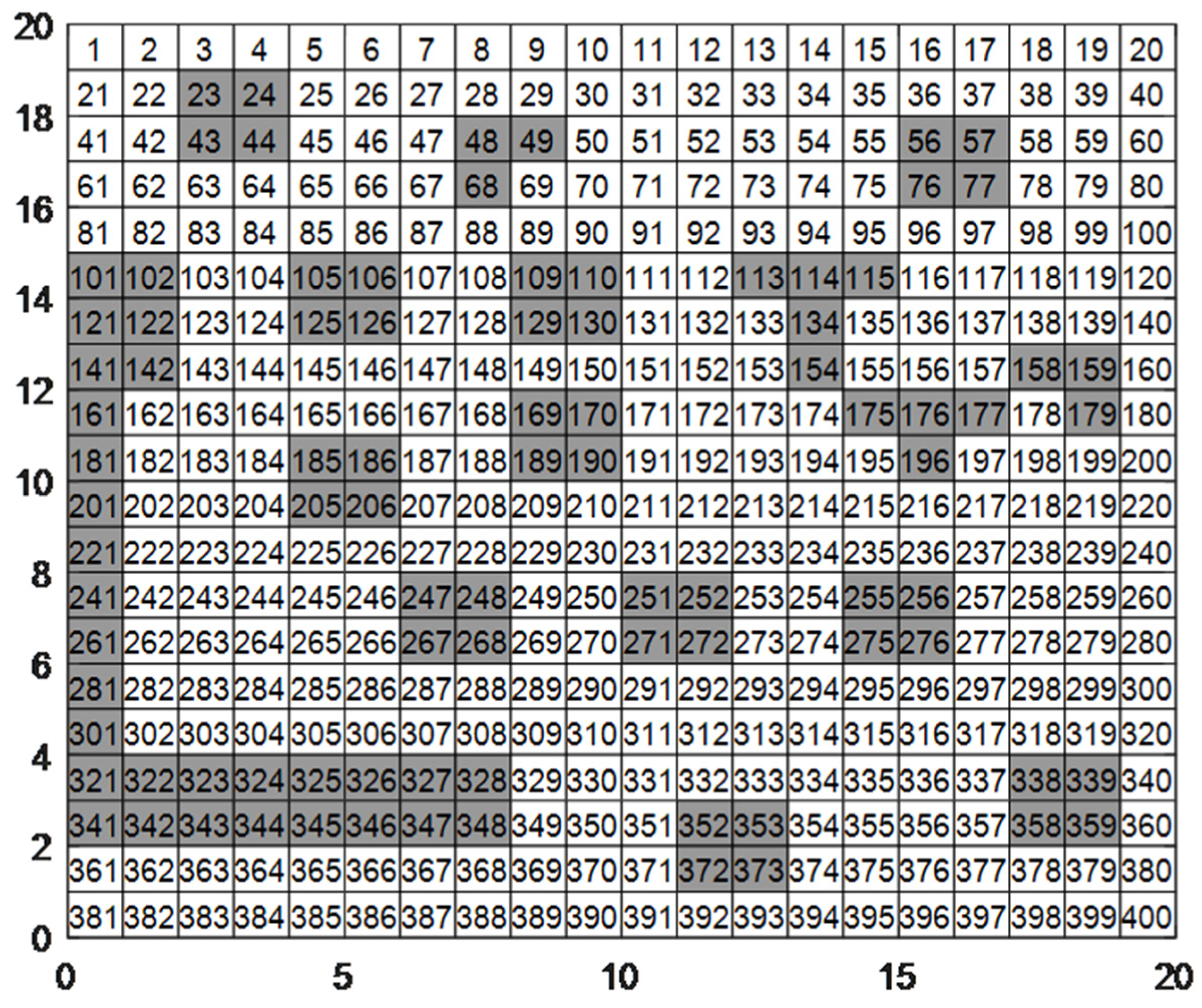
2. Environment Modeling

In this study, the grid method is chosen to establish the model of AGV. Assuming there are static obstacles in the environment, in order to prevent AGV from colliding with obstacles, if there are obstacles in the actual position corresponding to a grid in the grid environment, no matter whether the grid is completely covered by obstacles, the grid is coded as “1” and shown in the simulation diagram with black grid. If a grid faces no obstacles, then it is coded as “0” and displayed in the simulation with a white grid. At this time, the AGV is treated as a particle, and the side length of the unit grid is set to 1. This is shown in Figure 1.

Figure 1 illustrates the correlation that exists between Cartesian coordinates and grid identifiers. Grid numbers start as an increasing sequence, from the left side to the right side, from top to bottom, starting with the numbers 1, 2, and so on. The Cartesian system is set, with the due east direction representing the positive x-axis, and the due north direction representing the positive y-axis. The upper boundaries for the horizontal and the vertical coordinates are represented as MM. The grid number is assigned a unique identifier along with positional coordinates, thus creating a correlation between the grid number and the rectangular coordinates:

$$\left\{\begin{array}{l}{x}_i=a_0(\mathrm{mod}(i,MM)-0.5)\\ y_i=a_0(MM+0.5-ceil(i/MM))\end{array}\right.$$

(1)

In Formula (1), i indicates the serial number code corresponding to the grid; MM indicates the number of rows or columns of a square grid map; (x_i,y_i) is the horizontal and vertical values corresponding to the i th cell in the grid. a₀ represents the side length of a unit of the grid; mod(i,MM) indicates the remainder of i/MM. ceil(i/MM) indicates that i/MM is rounded up.

In the process of AGV movement, there are eight movement directions, but the direction of the previous step needs to be removed, and the actual alternative direction is 7.

3. Basic Algorithms

3.1. ACA

The Ant Colony Optimization (ACO) is a biomimetic metaheuristic for optimization inspired by ant colonies’ foraging behavior in their ecosystems. The technique has its roots in the work of Dorigo et al. in the 1990s. The basic idea behind the application of the ACO is the cooperative way ants create routes through the deposition of pheromones; when foraging, ants choose paths randomly and deposit pheromones indicating more desirable routes upon returning to the nest. Consequently, ants that follow are likely to go through paths with higher pheromone levels, hence creating a self-organizing optimization process with positive feedback.

3.1.1. Path Selection Probability

In the traditional ACA, ants need to select movement paths. Relying on factors such as the ‘pheromone concentration (PC)’ on the path and the distance between nodes, they calculate the probability of transferring from the current node to other nodes through the state transition probability Formulas (2) and (3). In this way, when searching, one can choose an appropriate path, thereby better exploring and utilizing the space of solutions.

$$P_{ij}^k\left(t\right)=\left\{\begin{array}{l}{\displaystyle \frac{{[{\tau }_{ij}\left(t\right)]}^{\partial }\cdot {[{\eta }_{ij}\left(t\right)]}^{\beta }}{{\displaystyle \sum s\in allowe{d}_k{[{\tau }_{is}\left(t\right)]}^{\partial }\cdot {[{\eta }_{is}\left(t\right)]}^{\beta }}}},j\in allowe{d}_k\\ 0,j\notin allowe{d}_k\end{array}\right.$$

(2)

$${\eta }_{ij}\left(t\right)={\displaystyle \frac{1}{d_{ij}\left(t\right)}}$$

(3)

In Equations (2) and (3), P_ij^k(t) means the probability that the kth ant moves from node i to node j at time t; τ_ij(t) represents the PC on the path between nodes i and j at time t; η_ij(t) represents the distance HF; d_ij(t) represents the Euclidean distance between nodes i and j; allowed_k is the set of nodes that the kth (k = 1, 2, …, m) ant has not visited yet, that is, the nodes that can be chosen next; s is a certain city in the set of unvisited nodes (allowed_k); α is the importance factor of PC; and β is the importance factor of the distance HF.

3.1.2. Update PC

In the classical ant colony system, the global pheromone update operation is usually performed after each search iteration. Not only do the pheromones evaporate naturally, but the magnitude of evaporation also depends on the evaporation coefficient. Concurrently, every time an ant traverses any particular pathway, it emits fresh pheromones, and the amount deposited during each traversal is directly proportional to the length of the trail. The updated Formulas (4) and (5) modify the PC along the trails to guide the next ants towards optimal routes.

$${\tau }_{ij}(t+1)=(1-\rho ){\tau }_{ij}(t)+{\displaystyle {\sum }_{k=1}^m\Delta {\tau }_{ij}^k,0<\rho <1}$$

(4)

$$\Delta {\tau }_{\mathrm{ij}}^{\mathrm{k}}=\left\{\begin{array}{l}{\displaystyle \frac{Q}{L_{\mathrm{k}}}},The nth ant has passed along the path from i to j.\\ 0,\mathrm{Others}.\end{array}\right.$$

(5)

In Equations (4) and (5), τ_ij(t) represents the PC on the path between node i and node j at time t, ∆τ_ij^k is the new PC produced by the kth ant on this path, and τ_ij(t + 1) is the concentration for the next round; ρ is the evaporation factor of the pheromone; Q represents the total number of pheromones; and L_k is the total length of the path taken by ant k.

3.2. APF Method

3.2.1. Gravitational Potential Field

Here, we set the initial destination point as the origin of the gravitational potential field. which generates a force that attracts the robot toward this specific location. In fact, the function of a field of gravitational potential is generally described as:

$$U_{att}(q)={\displaystyle \frac{1}{2}}{k}_{att}{d}^2(q,q_{goal})$$

(6)

In Equation (6), q represents the current position (CP) of the robot, q_goal is the target point (TP), k_att is the gravitational coefficient, and d(q, q_goal) is the distance between the CP of the robot and the TP. The strength of the gravitational field (equivalent to gravitational force per unit mass) can be mathematically described as the spatial derivative that points in the direction opposite to the gradient of the scalar gravitational potential function.

$$F_{att}(q)=-\nabla U_{att}(q)=k_{att}(q_{goal}-q)$$

(7)

The attractive force acting on the robot diminishes nonlinearly as its proximity to the target position (TP) increases. At the point of spatial coincidence between the robot and the TP, this force field achieves an equilibrium state with vanishing magnitude.

3.2.2. Repulsive Potential Field (RPF)

The RPF is generated by obstacles and is used to prevent the robot from colliding with them. A common RPF function is expressed as:

$$U_{rep}(q)=\left\{\begin{array}{l}{\displaystyle \frac{1}{2}}{k}_{rep}{({\displaystyle \frac{1}{d(q,q_{obs})}}-{\displaystyle \frac{1}{q_0}})}^2,d(q,q_{obs})<q_0\\ 0,d(q,q_{obs})\ge q_0\end{array}\right.$$

(8)

In Equation (8), q_obs means the obstacle position, k_rep is the repulsive coefficient, q₀ is the threshold of the obstacle influence range, and d(q, q_obs) is the distance between the robot CP and the obstacle position. The repulsive force is the negative gradient of the RPF function:

$$F_{rep}(q)=\left\{\begin{array}{l}{k}_{rep}({\displaystyle \frac{1}{d(q,q_{obs})}}-{\displaystyle \frac{1}{q_0}}){\displaystyle \frac{1}{d^2(q,q_{obs})}}{\displaystyle \frac{(q-q_{obs})}{d(q,q_{obs})}},d(q,q_{obs})<q_0\\ 0,d(q,q_{obs})\ge q_0\end{array}\right.$$

(9)

The repulsive force will increase rapidly as the robot approaches the obstacle.

3.2.3. Resultant Force and Motion

The resultant force F(q) acting on the robot is the vector sum of the attractive force F_att(q) and the repulsive force F_rep(q), that is:

$$F(q)=F_{att}(q)+F_{rep}(q)$$

(10)

The robot adjusts its movement direction and speed based on the direction and magnitude of the resultant force it experiences. In an ideal situation, the robot will move towards the TP under the pull of gravity while avoiding obstacles due to the repulsive force.

4. ACA Integrated with the APF Method

4.1. Improvement of HF Based on the Attraction of APF

The HF has a crucial role in the ACA, as its selection directly influences the ants’ path selection behavior, and it affects the algorithm’s convergence efficiency and the quality of the final solution. In conventional ACAs, the HF is solely related to the Euclidean distance d_ij(t) between the current node i and the available node j. Initially, the differences among d_ij(t) are small, and the initial PC is uniformly distributed, leading to a high degree of blindness in the algorithm’s initial search and deficiencies in its optimization ability and convergence. Therefore, this paper improves the traditional HF η_ij(t). Considering that in a grid environment, obstacles can be avoided through grid attributes, and when the target attraction and obstacle repulsion act together, problems such as “unreachable target” and “local extremum trap” may occur, this paper eliminates the repulsive effect of obstacles and only considers the target attraction to create a potential field HF η_F(t), using the attraction in the APF to guide ants towards the TP. At the same time, the original distance HF formula is improved, replacing d_ij(t) with the Euclidean distance d_iE(t) from the current node i to the target node E, thereby enhancing the guidance of the target node to the current node and enabling the algorithm to find the optimal path more quickly. The improved way of expression is like the following:

$${\eta }_{ij}^{\prime }(t)={\eta }_F(t)\cdot {\eta }_d(t)$$

(11)

$${\eta }_F(t)=a^F$$

(12)

$$U={\displaystyle \frac{1}{2}}k{d}_{iE}^2$$

(13)

$$F=-grad(U)=-k{d}_{iE}$$

(14)

$${\eta }_d(t)={\displaystyle \frac{1}{d_{iE}(t)}}$$

(15)

In Equations (11)–(15), η_ij represents the improved HF; η_F(t) is the attraction potential field HF; η_d(t) is the distance HF; F is the APF attraction; a is the influence factor of the APF attraction; U is the gravitational potential field function; k is the gravitational gain coefficient; and d_iE(t) is the distance between the current node i and the target node E at time t.

4.2. Improvement of Pheromone Volatilization Factor ρ

The pheromone evaporation coefficient measures how much pheromone evaporates from the pathway taken. A numerical change will change how much the level of pheromone is on that path, which greatly affects ants’ decision-making behavior when selecting paths and the performance trajectory of the whole ant colony. In normal ACAs, it is kept at a constant value. If it is too large, the rate at which pheromone evaporates will become too fast and at risk of becoming stuck in a local optimum. If it is too small, then variations in concentrations of pheromone along paths will be less, resulting in slow convergence. We adjusted the regulation of pheromone by adopting a dynamic volatilization strategy—the dissipation rate of pheromone is automatically adjusted according to the search process. This adaptive mechanism not only effectively prevents the search process from stagnating in the suboptimal solution region but also significantly improves the exploration efficiency of the system in the solution space. The specific implementation mechanism is as follows:

$$\lambda =1-e^{-{\displaystyle \frac{N_c}{N_{\max }}}}$$

(16)

$${\rho }^{\prime }=\rho \times \lambda$$

(17)

In Equations (16) and (17), λ is the evaporation factor adjustment coefficient, and λ ∈ (0, 1); N_c is the current iteration number of the ant colony; and N_max is the maximum iteration number of the ant colony.

4.3. Improvement of the Pheromone Update Mechanism

During the operation of the traditional ant colony algorithm, as the search cycle becomes longer and longer, the pheromone content in the search space gradually accumulates. This accumulation of pheromones causes subsequent ants participating in the path finding to be more inclined to choose routes with higher PCs. As pheromones evaporate, those paths less frequently chosen by ants may gradually lose pheromones, which can very easily enable the algorithm to find a local optimal solution. In the current study, for a specific problem, an adaptive pheromone regulation strategy was designed. This strategy is based on the initial pheromone increment update mechanism. On this basis, the pheromone constant values carried by all ants on the optimal path in the previous generation’s optimization process are summarized and the pheromone constant values carried by all ants on the worst path in the same process are subtracted. By using this method, a new, self-adaptive pheromone update mode was successfully constructed, and the specific mathematical expressions are shown in Formulas (18)–(20).

$${\tau }_{ij}^{\prime }(t+1)=(1-\rho ){\tau }_{ij}(t)+{\displaystyle {\sum }_{k=1}^m\Delta {\tau }_{ij}^k+\Delta {\tau }_{ij}^g(t)-\Delta {\tau }_{ij}^w(t)}$$

(18)

$$\Delta {\tau }_{ij}^g(t)=\left\{\begin{array}{l}{\displaystyle \frac{b\times Q}{L_{\min }}},j\in T^g\\ 0,\mathrm{Others}\end{array}\right.$$

(19)

$$\Delta {\tau }_{ij}^w(t)=\left\{\begin{array}{l}{\displaystyle \frac{w\times Q}{L_{\max }}},j\in T^w\\ 0,\mathrm{Others}\end{array}\right.$$

(20)

In Equations (18)–(20), ∆_ij^g(t) represents the increase in PC on the optimal path between node i and node j at time t; ∆_ij^w(t) represents the increase in PC on the worst path between node i and node j at time t; b represents the number of ants that successfully find the optimal route; w corresponds to the number of individuals trapped in the inefficient path; and L_min and L_max record the extreme parameters of the planned path, respectively—the former represents the shortest feasible distance confirmed by the system, and the latter indicates the maximum detour length found in actual exploration.

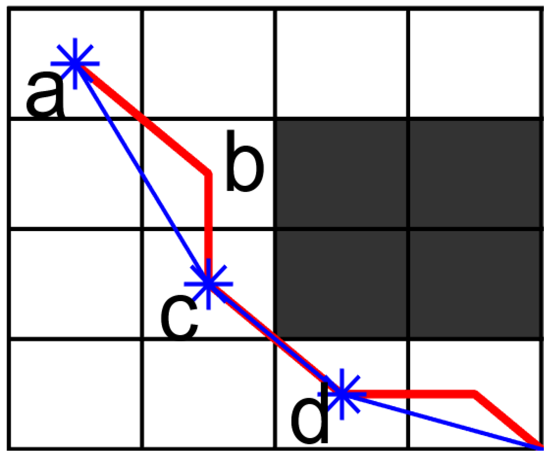
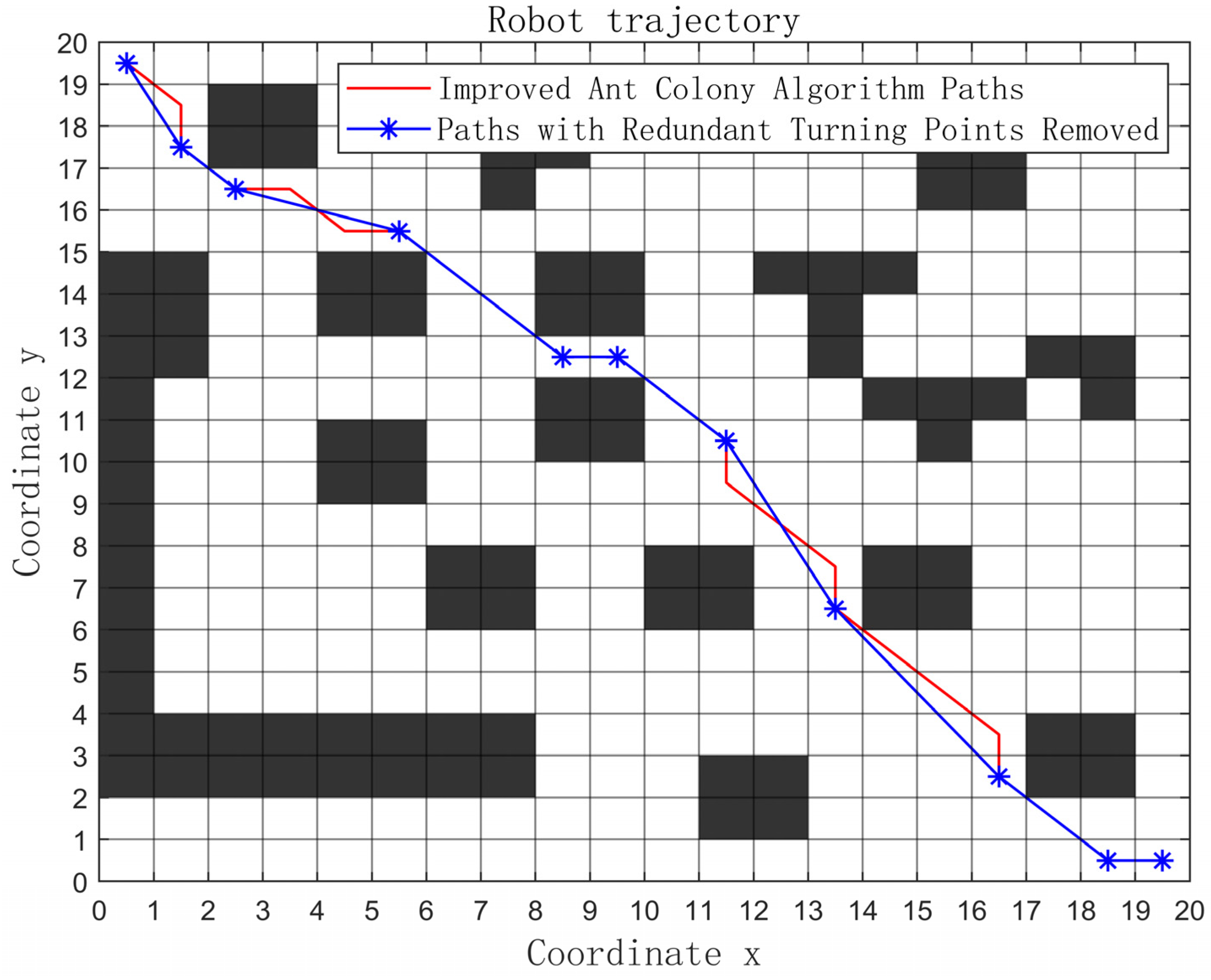
4.4. Pruning Method for Path Optimization and Update

To further reduce unnecessary turning points and shorten the path length, this paper adopts the pruning method to cut off redundant turning points for path optimization and update. Its principle is shown in Figure 2.

The unpruned path is a→b→c→d. Since there is no obstacle between a and c, the path a→c is used to replace a→b→c, and the redundant turning point b is pruned, resulting in the pruned path a→c→d. As there is an obstacle between points a and d, the path flows from point a to point c to point d, and keeps the inflection point c unchanged. In this way, the length of the path can be reduced and the path can be further optimized.

4.5. Algorithm Execution Process

Step 1: Establish a grid environment map model. Set the free grids as white grids and the obstacle grids as black grids. Define the starting map point as S and the end as E.

Step 2: Initialize relevant parameters. Set the initial values of parameters such as the maximum number of iterations K in the algorithm, the number of ants M in the ant colony, the importance factor α of PC, the importance factor β of the HF, and the evaporation factor ρ of pheromone.

Step 3: Perform the selection operation of path nodes. Based on the probability transfer formula, the stop should select the next node to visit from the available nodes and record the visited nodes in the taboo list. After each node selection, determine in real time whether the current ant has reached the target node. Continue following the operation steps just now until all the ants in this iteration have completed their path search.

Step 4: Record path length and ant quantity. Record the path length and the nodes passed by each ant in each iteration, and record the best path length, the worst path length and the number of ants passing through this path.

Step 5: Pheromone update. According to the data recorded in Step 4, update the PC according to the pheromone update mechanism.

Step 6: End of iteration process. Determine whether all iterations have been completed. If not, return to Step 3 to continue the operation; otherwise, store and output the optimal path obtained from this operation.

Step 7: Pruning optimization. Perform pruning operation on the optimal path obtained in Step 6 to remove redundant turning points and output the optimized path. The algorithm flowchart is shown in Figure 3.

5. Algorithm Simulation and Analysis

This research uses the Matlab R2022a development platform to realize the algorithm verification, and the running environment is the 64-bit operating system platform of Win7 system. The test device is equipped with an Intel Core i7-11800H CPU chip (The Intel Core i7—11800H CPU chip is manufactured by Intel5. Intel is an American multinational technology company headquartered in Santa Clara, CA, USA), the main frequency is 2.3 GHz, equipped with 31.8 GB of running memory. In order to evaluate the optimization effect, two raster map examples of different scales, 20 × 20 and 30 × 30, were constructed to carry out comparative tests.

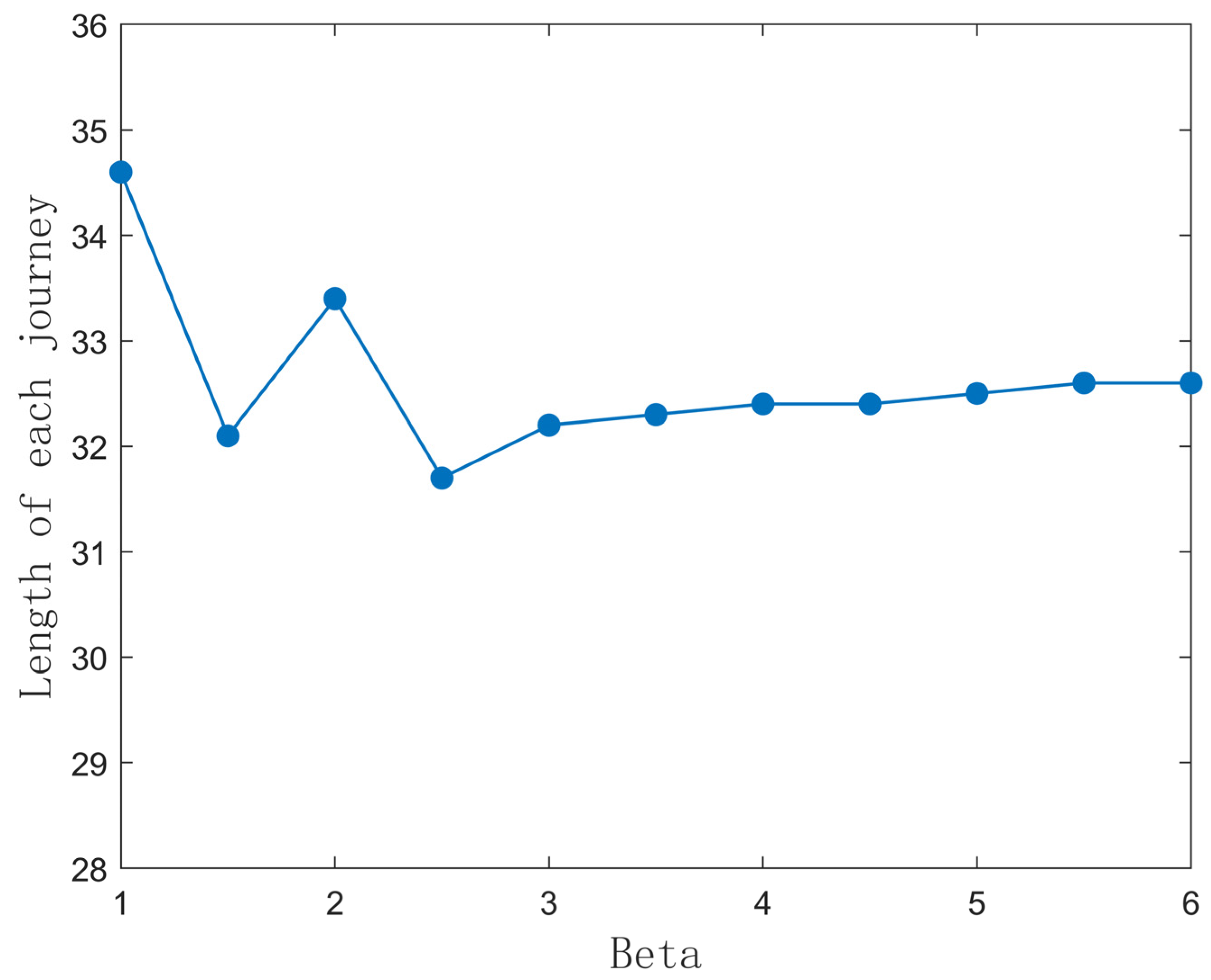
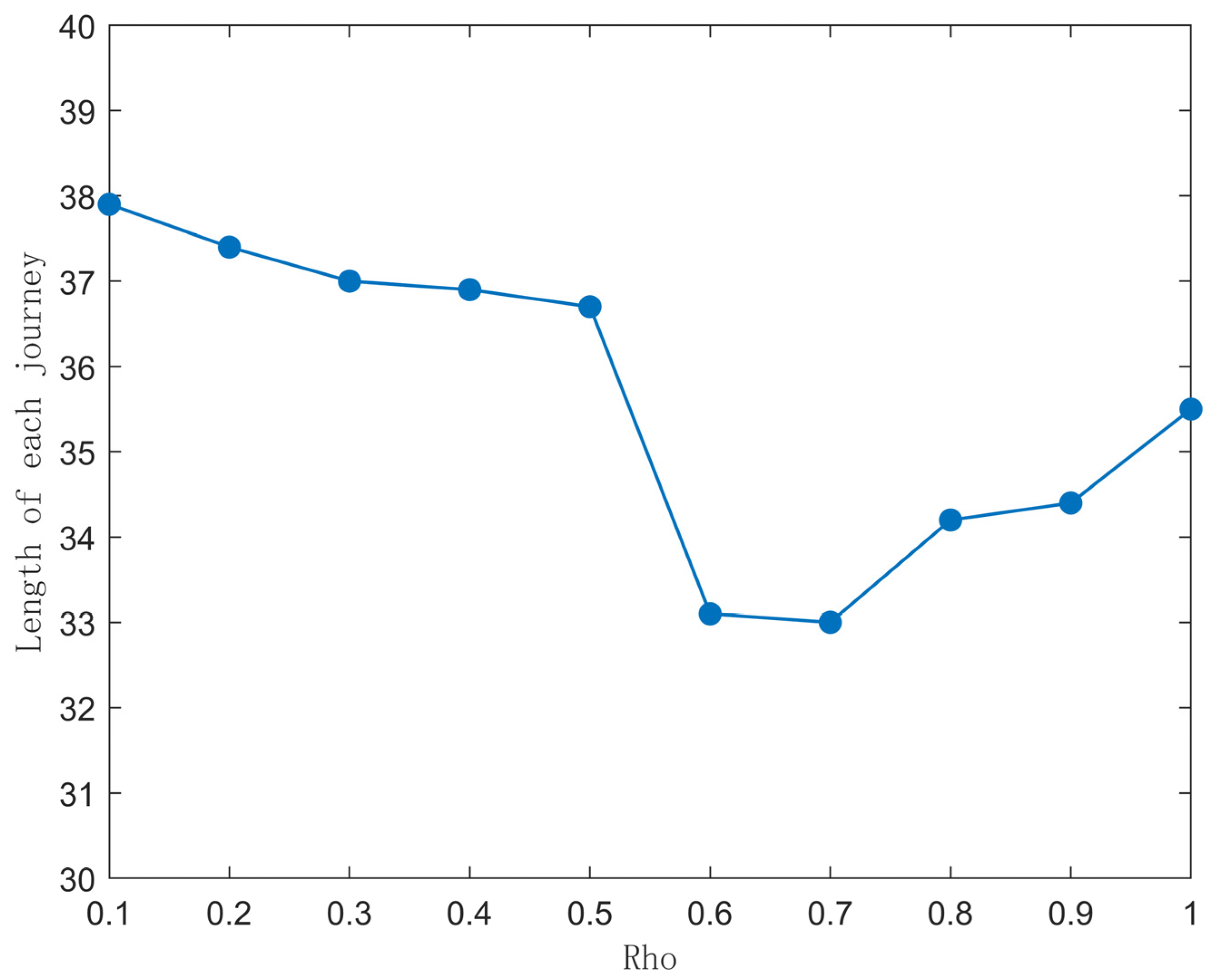
5.1. Parameter Sensitivity Analysis

The optimal selection of parameters in the ant colony algorithm does not have rigorous theoretical support at present and mainly depends on the statistical data as well as experience accumulation. However, the important parameters in the algorithm, such as the heuristic factor and the number of ant colonies, will have an important impact on the advantages and disadvantages of the results of the path planning; therefore, it is of great significance to analyze the sensitivity of the parameters.

In this paper, we use the control variable method to simulate the number of ants, the information heuristic factor, the expected value heuristic factor and the volatility coefficient in the ant colony algorithm, in which the original parameters are set as m = 30, α = 1, β = 5, ρ = 0.25. In order to ensure the reliability of the experimental results, we repeat the experiments 50 times to obtain the average value of each group of parameters and analyze the changes in the path length by changing the values of the parameters. To ensure the reliability of the experimental results, the average value of each set of parameters is obtained by repeating the experiment 50 times, and the change of the path length is analyzed by changing the parameter values.

From Figure 4, it can be seen that when the number of ants is 50, the path is the shortest, and with an increase in the number, the obtained solution stabilizes around it. Considering the time complexity and the convergence speed of iteration, it is most appropriate to choose the ant colony number of 50; from Figure 5, it can be seen that when α < 1, the path gradually converges to the optimal solution with the increasing value; from Figure 6, it can be seen that β should not be taken too small; in Figure 6, the minimum value should not be taken too small, the maximum value should not be taken too large, and the length of the path and the number of iteration are better; from Figure 7, it can be seen that ρ is not suitable to be taken too large or too small.

After the sensitivity analysis of the main parameters of the algorithm, the key configuration parameters selected for the specific test scenarios are listed in

Table 1. Configuration of basic parameters for simulation experiments.

Parameter	Letter Code	Value
Ant population	M	50
Iteration times	K	200
Importance factor of PC	α	1
Importance factor of HF	β	4
Pheromone evaporation degree factor	ρ	0.7
Total pheromone amount	Q	10
Influence factor of APF attraction	a	0.3
Gravity gain coefficient	k	0.01

.

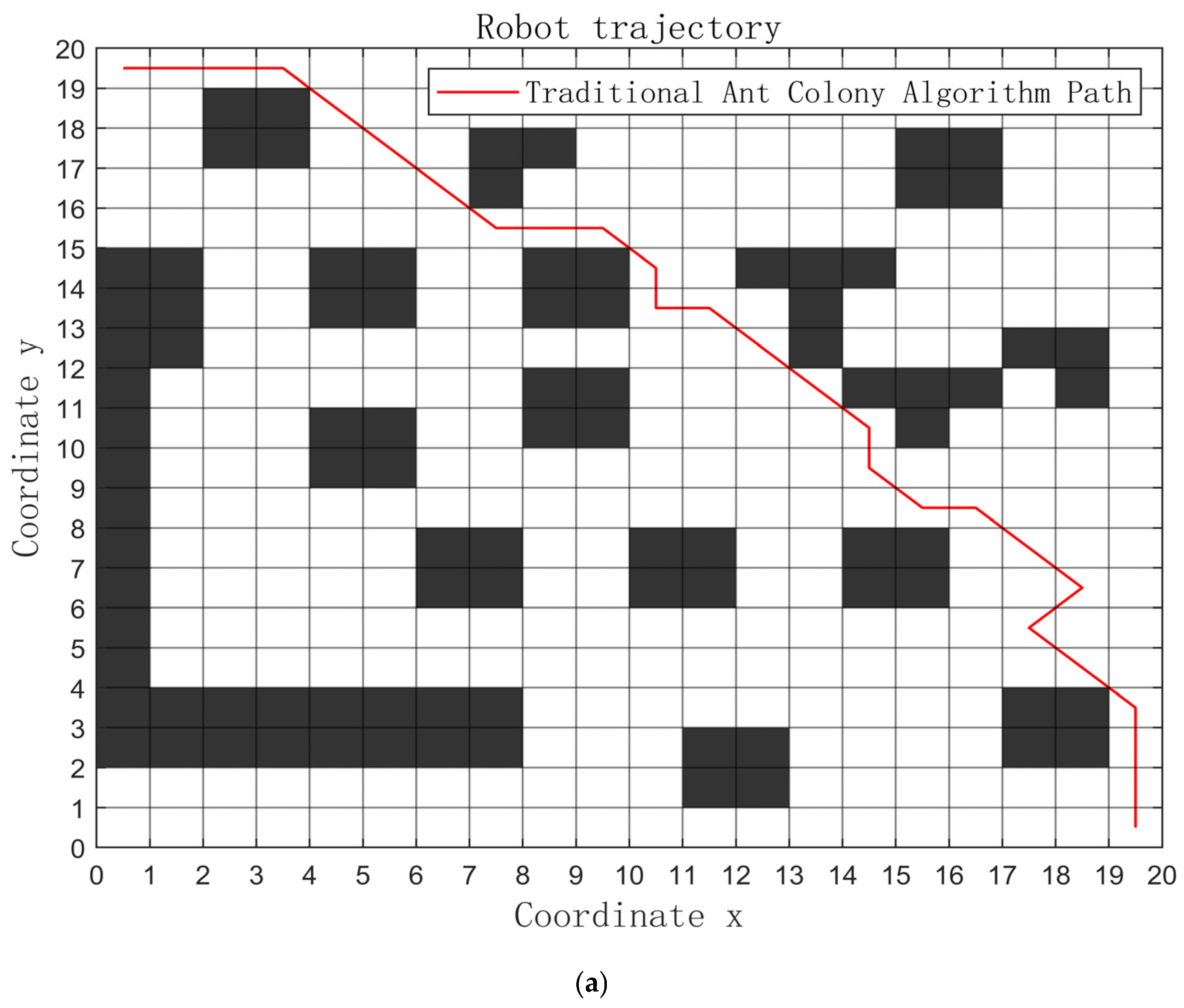
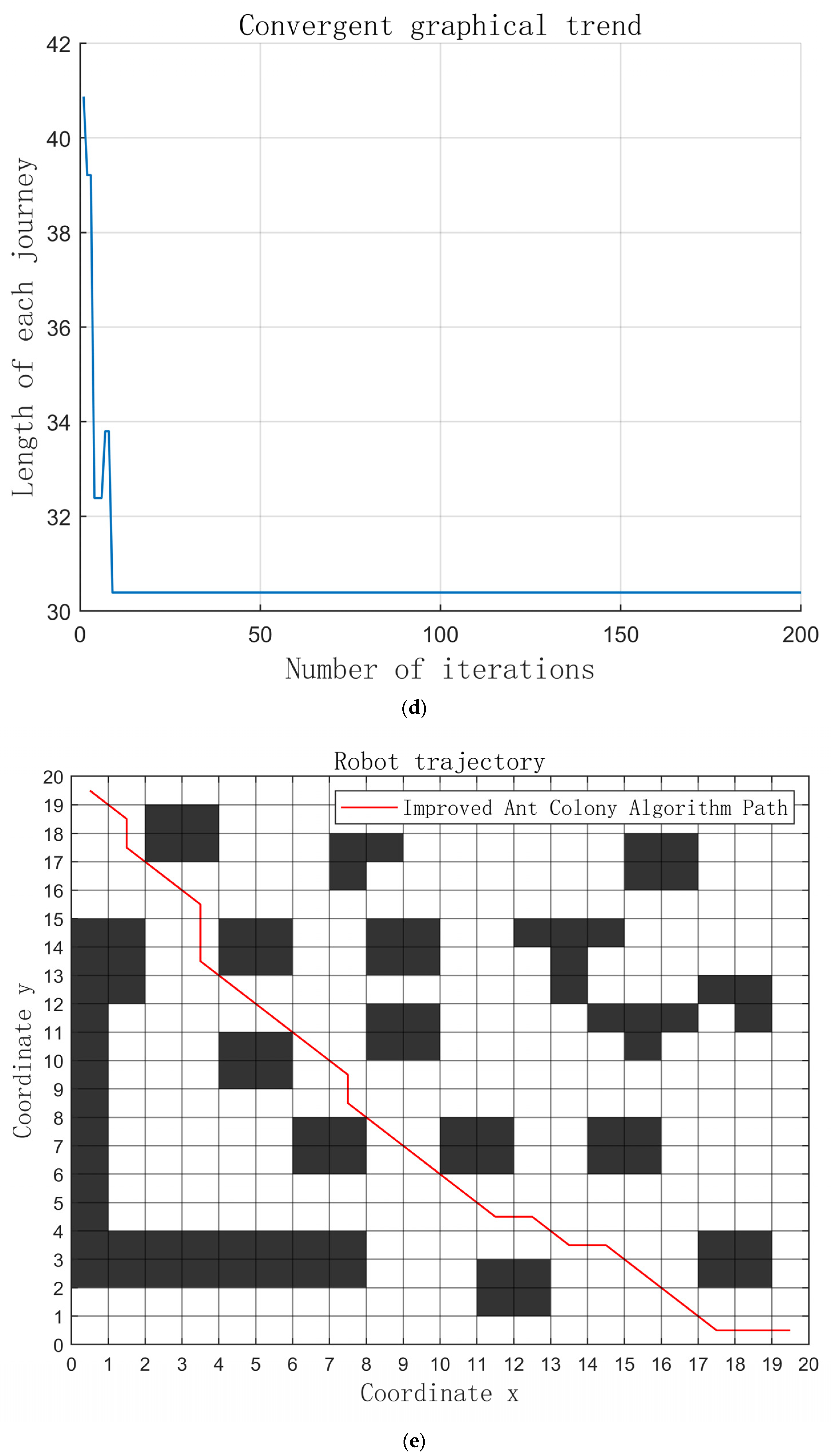
5.2. A 20 × 20 Grid Map

Firstly, a 20-order grid matrix was simulated, with the obstacle distribution randomly set. The starting node was set as the grid with the serial number 1, with coordinates (0.5, 19.5), and the target node was set as the grid with the serial number 400, with coordinates (19.5, 0.5). In order to verify the validity of the algorithm proposed in this paper, this study conducted simulation experiments on the traditional ACA, the GA–ACA proposed in the literature [25] and the improved ACA after optimizing the HF, the pheromone evaporation factor and the pheromone updating mechanism. The robot path trajectory graphs and convergence curve graphs were obtained by simulating the experimental process of the three algorithms with rigorous parameter settings and operations, and each algorithm was run 100 times to find the optimal path. These experimental results are shown in Figure 8, which visualizes the performance of different algorithms in PP.

In Figure 8, the conventional ACA forms a zigzag path trajectory, whereas the GA–ACA and the improved ACA proposed in the literature [25] tend to use the diagonal path of the grid. Meanwhile, the path obtained by the improved ACA has fewer corners compared to GA–CA. Therefore, the algorithm proposed in this study can find shorter, smoother and faster converging paths.

HF improvement, pheromone evaporation factor, and pheromone update mechanisms, as detailed in

Table 2. Comparison of the results of simulation experiments in a 20 × 20 grid environment.

Algorithm	Shortest Path Length	Convergent Iteration Times	Path Turning Points	Running Time
Traditional ACA	31.80	81	13	25.35
ACA fused with GA	30.38	9	12	9.80
ACA fused with APF	29.21	7	11	5.16

, are evidenced by comparing them with a conventional ACA and GA–ACA when resolving path problems that the upgraded performance ACA has successfully surpassed. Compared with the traditional algorithm, the advanced path optimization method reduces the path length by 8.14%, the number of convergence iterations by 91.36%, the path turning points by 15.38%, and the running time by 61.34%. Compared to GA–ACA, the advanced path optimization method reduces the path length by 3.85%, the number of convergence iterations by 22.22%, the path turning points by 8.33%, and the runtime by 47.35%.

As shown in Figure 9, after the excessive turning points were removed using pruning, the shortest path was further shortened from 29.2132 to 27.7433, bringing the number of turning points along the path down to four. The path length was optimized by 5.03%, while the number of turning locations dropped by 63.64%.

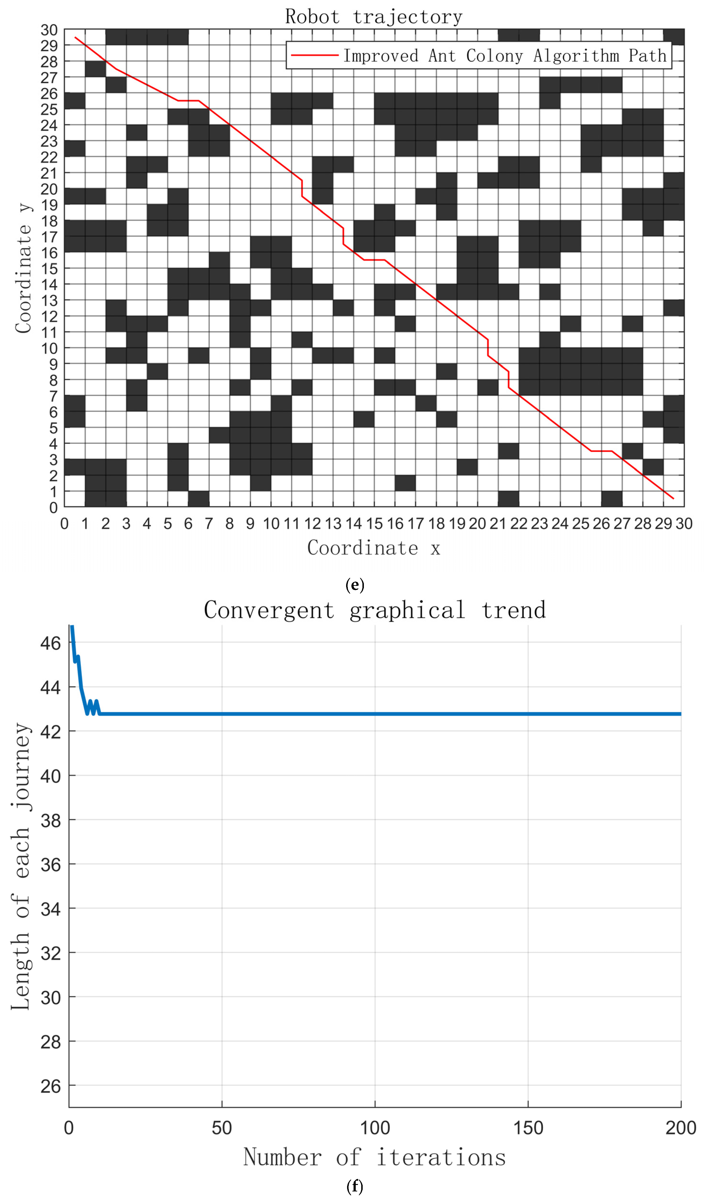
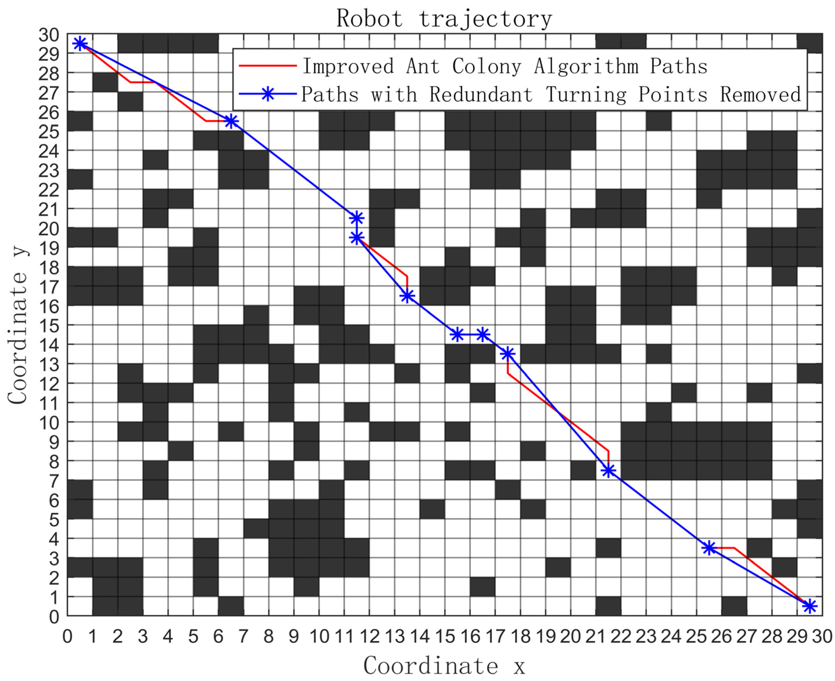
5.3. A 30 × 30 Grid Map

To conduct a comparison of the performance differences between the improved ACA and the traditional ACA, this paper sets up a more complex grid environment for further experiments. The map size is set to 30 × 30, and the obstacles are more densely distributed. The starting node is set as the grid with the number 1, with coordinates (0.5, 29.5), and the target node is set as the grid with the number 900, with coordinates (29.5, 0.5). In this study, to comprehensively evaluate the algorithm performance, simulation experiments are conducted, respectively, for the classic ACA, the GA–ACA algorithm proposed in the literature [25] and the optimized ACA. The experiments precisely simulate the robot’s operation under the guidance of different algorithms through specific simulation environments and parameter settings. Each algorithm was run 100 times and the optimal result was taken. Ultimately, the robot path trajectory diagrams and convergence curve diagrams obtained from the experiments are uniformly organized and presented in Figure 10 for intuitive comparison and analysis of the performance of the three algorithms in PP.

As can be seen from Figure 10, when the environmental complexity continuously increases, the path trajectory planned by the traditional ACA shows more pronounced zigzag patterns, which greatly affect the smoothness and rationality of the path. However, GA–ACA and the improved ACA still prefer to take the diagonal paths of the grids. Meanwhile, the path obtained by the improved ACA has fewer corners compared to GA–ACA. In more complex grid environments, the algorithm proposed in this study demonstrates significant advantages, being able to find shorter and smoother paths. At the same time, the convergence speed of the algorithm is also faster, and the PP task is effectively completed.

By improving the HF, pheromone evaporation factor, and pheromone updating mechanism,

Table 3. Comparison of the results of simulation experiments in a 30 × 30 grid environment.

Algorithm	Shortest Path Length	Convergent Iteration Times	Path Turning Points	Running Time
Traditional ACA	49.60	133	20	124.73
ACA fused with AG	44.80	86	17	24.97
ACA fused with APF	43.36	16	16	7.53

shows that the improved ACA reduces the shortest path length by 12.58%, the number of convergence iterations by 87.97%, the number of path turning points by 20%, and the runtime by 79.98% compared to the conventional ACA. Compared to GA–ACA, the improved ACA reduces the path length by 3.21%, the number of convergence iterations by 81.40%, the path turning points by 5.88%, and the running time by 69.84%.

As shown in Figure 11, after path optimization, unnecessary direction adjustment points in the original trajectory are effectively eliminated. After optimization, the system records show that the optimal moving distance is shortened from 43.35 units to 41.99 units, and the trajectory turning point is shortened from the initial 16 points to 9 points. The improved effect is reflected in the movement efficiency increased by 3.13%, and the direction adjustment frequency decreased significantly by 43.75%.

6. Conclusions

This study proposes an AGV PP method that combines the APF algorithm with the ACA, making four improvements and innovations on the basis of the traditional ACA. In the algorithm optimization process of this study, an attraction function is added to the initial HF, which makes the target node have a stronger guiding effect on the ants performing the path-finding task, significantly improving the efficiency of the algorithm’s convergence and accelerating the solution process. Considering the dynamic characteristics of the algorithm’s iterative process, a method of flexibly adjusting the pheromone evaporation factor based on the number of iterations is adopted. This dynamic adjustment mechanism effectively expands the search range and greatly enhances the algorithm’s ability to screen high-quality solutions in the entire space, comprehensively improving the algorithm’s performance in solving complex problems. In the pheromone update process, a reward and punishment mechanism is added, and multiple parameters are used to dynamically adjust the pheromone increment, strengthening the guiding role of superior ants and weakening the misleading effect of inferior ants, thus avoiding getting trapped in local optima as much as possible. Finally, this paper uses the pruning method to further optimize the path, reducing unnecessary turning points, increasing the smoothness of the path, reducing unnecessary turns, and significantly reducing the overall length of the path.

Through experiments on the improved ACA in grid environments of different complexities and comparisons with the traditional ACA in multiple aspects, the efficiency and stability of the algorithm proposed in this paper were verified. Subsequent localized path-planning studies will be conducted in conjunction with unknown environments and dynamic obstacles.

References

1. Liu, H.; Luo, J.; Zhang, L.; Yu, H.; Liu, X.; Wang, S. Research on Traversal Path Planning and Collaborative Scheduling for Corn Harvesting and Transportation in Hilly Areas Based on Dijkstra’s Algorithm and Improved Harris Hawk Optimization. Agriculture 2025, 15, 233. [Google Scholar] [CrossRef]
2. Zhang, C. An Improved Dijsktra Algorithm and Its Implementation in GIS. Comput. Appl. Softw. 2011, 28, 275–277. [Google Scholar]
3. Liu, L.; Wang, B.; Xu, H. Research on Path-Planning Algorithm Integrating Optimization A-Star Algorithm and Artificial Potential Field Method. Electronics 2022, 11, 3660. [Google Scholar] [CrossRef]
4. Yin, X.; Cai, P.; Zhao, K.; Zhang, Y.; Zhou, Q.; Yao, D. Dynamic Path Planning of AGV Based on Kinematical Constraint A* Algorithm and Following DWA Fusion Algorithms. Sensors 2023, 23, 4102. [Google Scholar] [CrossRef] [PubMed]
5. Zhang, C.; Huang, P.; Zhang, G.; Jin, Z.; Chen, Y.; Zong, M.; Chi, J.; Qiu, Z. Research on Adaptive Path Planning Based on Improved A* Algorithm. Commun. Inf. Technol. 2025, 1, 43–45+122. [Google Scholar]
6. Sun, P.; Liu, C.; Shi, X.; Zhang, H.; Zha, W. Research on Path Planning for Mobile Robots Based on Improved A* Algorithm [J/OL]. J. Heilongjiang Inst. Technol. 2025, 1–8. Available online: http://kns.cnki.net/kcms/detail/23.1498.N.20250115.1809.004.html (accessed on 1 March 2025).
7. Zhang, Q. Design of Data Mining Method for Logistics Engineering Based on A* Algorithm and Cluster Analysis. J. Guiyang Univ. (Nat. Sci. Ed.) 2024, 19, 45–48+56. [Google Scholar]
8. Chi, X.; Li, H.; Fei, J. Research on Random Obstacle Avoidance Method for Robots Based on Improved A* Algorithm and Dynamic Window Approach. J. Instrum. 2021, 42, 132–140. [Google Scholar]
9. Kang, J.-G.; Lim, D.-W.; Choi, Y.-S.; Jang, W.-J.; Jung, J.-W. Improved RRT-Connect Algorithm Based on Triangular Inequality for Robot Path Planning. Sensors 2021, 21, 333. [Google Scholar] [CrossRef]
10. Fu, J.; Mu, L.; Di, X.; Zhang, X.; Zhang, H. Research on Complex Obstacle Avoidance Path Planning for Manipulators Based on Improved RRT Algorithm. Mod. Electron. Technol. 2025, 48, 180–186. [Google Scholar]
11. Zhou, R.; Liu, H.; Peng, X. Intelligent Vehicle Path Planning Strategy Based on Optimized RRT Algorithm. Softw. Eng. 2024, 27, 49–52. [Google Scholar]
12. He, X.; Zhou, Y.; Liu, H.; Shang, W. Improved RRT*-Connect Manipulator Path Planning in a Multi-Obstacle Narrow Environment. Sensors 2025, 25, 2364. [Google Scholar] [CrossRef]
13. Wang, J.; Li, T.; Li, B.; Meng, M.Q.-H. GMR-RRT*: Sampling-based Path Planning Using Gaussian Mixture Regression. IEEE Trans. Intell. Veh. 2022, 7, 690–700. [Google Scholar] [CrossRef]
14. Teng, Y.; Feng, T.; Song, C.; Li, J.; Yang, S.X.; Zhu, H. Path Planning of Mobile Robot Based on Dual-Layer Fuzzy Control and Improved Genetic Algorithm. Symmetry 2025, 17, 609. [Google Scholar] [CrossRef]
15. Zhang, Z.; Yang, H.; Bai, X.; Zhang, S.; Xu, C. The Path Planning of Mobile Robots Based on an Improved Genetic Algorithm. Appl. Sci. 2025, 15, 3700. [Google Scholar] [CrossRef]
16. Liu, C. Multi-UAV Route Planning Method Based on Improved Genetic Algorithm. Fire Control Command. Control 2019, 44, 18–22. [Google Scholar]
17. Song, Y.; Gao, G.; Liang, C.; Xu, J. Path Planning of Unmanned Aerial Vehicles Based on Multi-Strategy Improved Grey Wolf Algorithm. Electron. Meas. Technol. 2025, 48, 84–91. [Google Scholar]
18. Liu, G.; Jin, S.; Li, Z.; Liu, B. Path Planning of Urban Passenger Electric Vertical Takeoff and Landing Aircraft Based on Improved Artificial Electric Field Algorithm. Sci. Technol. Eng. 2025, 25, 238–244. [Google Scholar]
19. Xue, M.; Xu, H.; Wang, S. Path Planning of Unmanned Surface Vessels Based on Particle Swarm Optimization Algorithm. China Sci. Technol. Inf. 2018, 24, 69–70. [Google Scholar]
20. Deng, D.; Xu, J.; Meng, H.; Yang, W. Path Planning of Mobile Robots Based on the Fusion of Ant Colony Algorithm and Artificial Potential Field Method. J. Instrum. Instrumnetation 2025, 1–16. [Google Scholar] [CrossRef]
21. Luo, Z.; He, G.; Zheng, X.; Huang, Y. Research on Robot Path Planning Based on Improved Ant Colony Hybrid Algorithm. J. Kunming Univ. Sci. Technol. (Nat. Sci. Ed.), 2025; 1–11. [Google Scholar] [CrossRef]
22. Wang, Y.; Shen, D.; Li, Y.; Li, J. AGV Path Planning Based on the Fusion of Jump Point Search and Bidirectional Ant Colony Algorithm. J. Xi’an Polytech. Univ. 2021, 35, 37–43. [Google Scholar]
23. Jiao, Z.; Ma, K.; Rong, Y.; Wang, P.; Zhang, H.; Wang, S. A path planning method using adaptive polymorphic ant colony algorithm for smart wheelchairs. J. Comput. Sci. 2018, 25, 50–57. [Google Scholar] [CrossRef]
24. Lu, D.; Wu, S. Robot Path Planning Based on Potential Field Ant Colony Algorithm. Syst. Eng. Electron. 2010, 32, 1277–1280. [Google Scholar]
25. Kong, X. Research on Global Path Planning Algorithm for Mobile Robots Integrating Ant Colony Algorithm and Genetic Algorithm. Master’s Thesis, Northeastern University, Boston, MA, USA, 2018. [Google Scholar] [CrossRef]
26. Stutzle, T.; Hoos, H.H. MAX-MIN Ant System. Future Gener. Comput. Syst. 2000, 16, 889–914. [Google Scholar] [CrossRef]
27. Pan, J.; Wang, X.; Cheng, Y. Path Planning of Mobile Robots Based on Improved Ant Colony Algorithm. J. China Univ. Min. Technol. 2012, 41, 108–113. [Google Scholar]
28. Yu, J.; Li, R.; Zhao, A.; Yu, Z.; Wang, J. Research on Path Planning of Warehouse AGV Based on Parallel Sorting Ant Colony Algorithm. Mech. Sci. Technol. 2021, 40, 609–618. [Google Scholar]
29. Liu, L.; Yuan, G.; Dai, Y. Multi-Ant Colony Pseudo-Parallel Optimization Algorithm. Comput. Eng. 2007, 23, 199–201. [Google Scholar]
30. Jin, D.; Yang, B.; Liu, J.; Liu, D.; He, D. Cluster Structure Detection in Complex Networks: An Ant Colony Algorithm Based on Random Walk. J. Softw. 2012, 23, 451–464. [Google Scholar] [CrossRef]
Figure 1. Grid environment.
Applsci 15 04522 g001
Figure 2. Example of path optimization.
Applsci 15 04522 g002
Figure 3. Flow chart of improved ACA.
Applsci 15 04522 g003
Figure 4. Effect of parameter M on path length.
Applsci 15 04522 g004
Figure 5. Effect of parameter α on path length.
Applsci 15 04522 g005
Figure 6. Effect of parameter β on path length.
Applsci 15 04522 g006
Figure 7. Effect of parameter ρ on path length.
Applsci 15 04522 g007
Figure 8. Comparative simulation experiment results in a 20 × 20 grid environment: (a) simulation movement trajectory of traditional ACA (20 × 20); (b) simulation convergence curve of traditional ACA (20 × 20); (c) simulation of motion trajectories using ACA integrated with GA (20 × 20); (d) convergence curve of ACA integrated with GA (20 × 20); (e) simulation of motion trajectories using ACA integrated with APF (20 × 20); (f) convergence curve of ACA integrated with APF (20 × 20).
Applsci 15 04522 g008aApplsci 15 04522 g008bApplsci 15 04522 g008cApplsci 15 04522 g008d
Figure 9. Results of pruning processing in a 20 × 20 grid environment.
Applsci 15 04522 g009
Figure 10. Comparative simulation experiment results in a 30 × 30 grid environment: (a) simulation movement trajectory of traditional ACA (30 × 30); (b) simulation convergence curve of traditional ACA (30 × 30); (c) simulation of motion trajectories using ACA integrated with AG (30 × 30); (d) convergence curve of ACA integrated with AG (30 × 30); (e) simulation of motion trajectories using ACA integrated with APF (30 × 30); (f) convergence curve of ACA integrated with APF (30 × 30).
Applsci 15 04522 g010aApplsci 15 04522 g010bApplsci 15 04522 g010c
Figure 11. Results of pruning in a 30 × 30 grid environment.
Applsci 15 04522 g011