Performance Analysis of Downlink 5G Networks in Realistic Environments

Abstract

Fifth-generation (5G) networks are the fifth generation of mobile networks and are regarded as a global standard, following 1G, 2G, 3G, and 4G networks. Fifth-generation, with its large available bandwidth provided by mmWave, not only provides the end user with higher spectrum efficiency, massive capacity, low latency, and high speed but is also a network designed to connect virtually everyone and everything together, including machines, objects, and devices. Therefore, studies of such systems’ performance evaluation and capacity bounds are critical for the research community. Furthermore, the performance of these systems should be investigated in realistic contexts while considering signal strength and restricted uplink power to maintain system coverage and capacity, which are also affected by the environment and the value of the service factor parameter. However, any proposed application should include a multiservice case to reflect the true state of 5G systems. As an extension of previous work, the capacity bounds for 5G networks are derived and analyzed in this research, considering both single and multiservice cases with mobility. In addition, the influence of different parameters on network performance, such as the interference, service factor, and non-orthogonality factors, and cell radii, is also discussed. The numerical findings and analysis reveal that the type of environment and service factor parameters have the greatest influence on system capacity and coverage. Subsequently, it is shown that the investigated parameters have a major impact on cell performance and therefore can be considered key indicators for mobile designers and operators to consider in planning and designing future networks. To validate these findings, some results are evaluated against ITU-T standards, while others are compared with related studies from the literature.

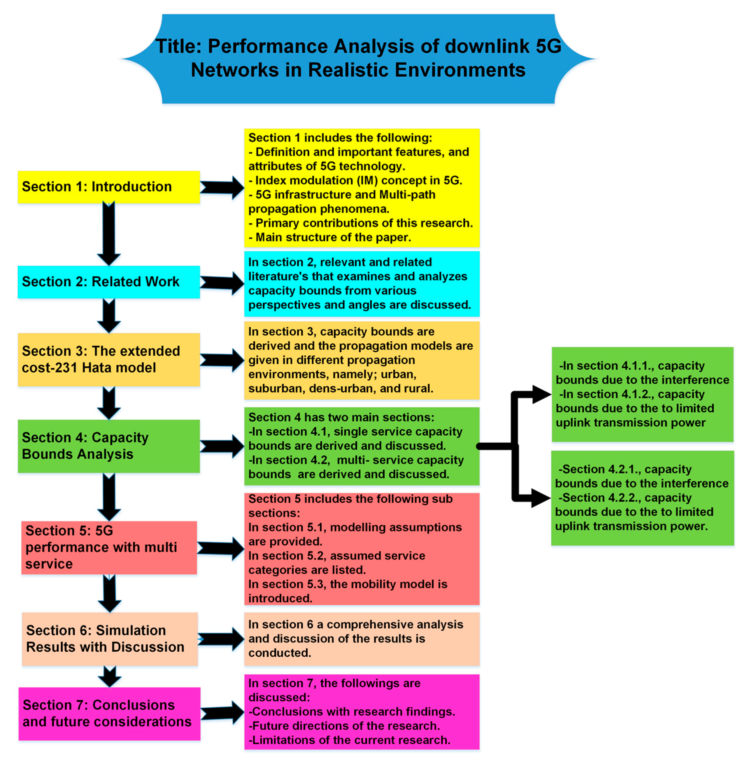
1. Introduction

Fifth-generation (5G) technology, known as the fifth generation of wireless technology, represents the most recent progress in mobile communications and networking. It signifies a considerable advancement in speed, capacity, latency, and connectivity relative to earlier generations (like 4G or LTE). Below are the important features and attributes of 5G technology:

• Enhanced Speed: Fifth-generation provides much faster data transfer rates compared to earlier generations, achieving peak speeds of up to 10 gigabits per second (Gbps). This allows for quicker downloads, uninterrupted streaming of high-definition material, and real-time interactions with minimal delay.
• Low Latency: Fifth-generation technology minimizes network latency to as little as 1 millisecond (ms), enabling nearly immediate communication between devices and reducing delays. This is essential for applications such as self-driving cars, telemedicine, and live gaming.
• High Capacity: Fifth-generation networks are capable of supporting a large number of connected devices at the same time. The technology employs advanced frequency bands, such as higher-frequency millimeter waves, to enhance network capacity and support the increasing number of Internet of Things (IoT) devices.
• Improved Coverage: Fifth-generation networks use a range of technologies, such as small cells, massive MIMO (multiple-input multiple-output), and beamforming, to enhance coverage and signal strength. This allows for dependable connectivity even in densely populated areas and isolated locations.
• Network Slicing: Fifth-generation brings in the idea of network slicing, enabling network operators to develop several virtual networks within one physical framework. Each network slice can be tailored to fulfill the unique needs of various applications, sectors, or user groups.
• Enhanced Energy Efficiency: Fifth-generation technologies are designed to be more energy-efficient than earlier generations. This is accomplished by the means of optimized network architecture, decreased power usage of network equipment, and smart network management.
• Fifth-generation is anticipated to play a crucial role in facilitating emerging technologies like autonomous vehicles, augmented reality (AR), virtual reality (VR), smart cities, industrial automation, and remote telemedicine. Fifth-generation networks meet the requirements of these advanced applications through their high speeds, low latency, and extensive connectivity.

Furthermore, some new technologies to improve coverage and capacity are provided by 5G and beyond. In this regard, Index Modulation (IM) [1,2,3] is a groundbreaking approach that aims to improve the spectral and energy efficiency of wireless communication systems, which is especially pertinent for 5G and subsequent technologies. IM holds great promise for 5G, providing notable enhancements in both spectral and energy efficiency. By utilizing the indices of various communication elements, IM is capable of meeting the varied and challenging demands of contemporary wireless networks, thereby serving as a crucial element in the advancement of 5G and future communication technologies. Below is a comprehensive overview of its key features.

• Spectral Efficiency: IM improves spectral efficiency by conveying additional information through the indices of various communication entities such as antennas, subcarriers, and time slots [4,5,6]. This allows for more data to be transmitted without increasing the bandwidth.
• Energy Efficiency: By selectively activating certain communication elements, IM reduces power consumption, which is crucial for the energy demands of 5G networks [5,6,7].

There are three types of IM:

• Spatial Modulation (SM): Utilizes the indices of antennas to transmit additional bits of information. This technique is particularly useful in multiple-input multiple-output (MIMO) systems [6,7].
• Orthogonal Frequency Division Multiplexing with Index Modulation (OFDM-IM): Combines OFDM with IM by activating a subset of subcarriers to carry information, enhancing both spectral efficiency and bit error rate (BER) performance [6,8,9].
• Generalized Frequency Division Multiplexing with Index Modulation (GFDM-IM)**: Extends the concept of IM to GFDM systems, offering better error performance and flexibility in multicarrier systems [10,11].

Moreover, IM has the following applications in 5G systems:

• Enhanced Mobile Broadband (eMBB): IM techniques can support high data rates and improved spectral efficiency, which are essential for eMBB services [7].
• Massive Machine-Type Communications (mMTCs): The energy efficiency of IM makes it suitable for mMTCs, where numerous devices require low-power communication [7].
• Ultra-Reliable Low-Latency Communication (URLLC): IM can help achieve the low latency and high reliability required for URLLC applications by optimizing resource usage [7].

It is essential to acknowledge that the rollout and accessibility of 5G networks and services differ from one region and country to another. Network operators are slowly implementing 5G infrastructure, and the complete potential of 5G technology is anticipated to be achieved gradually as additional devices, applications, and industries take advantage of its features.

The term “cells” refers to the small hexagonal geographic areas that constitute 5G networks, which are the fifth generation of cellular networks. Before the final deployment of 5G, as described in [12], research centers must manage certain needs. Therefore, mobile operators are battling to increase their capacity without sacrificing the quality of service (QoS) to address the issue of a lack of resources [13].

Fifth-generation network infrastructure is built on the millimeter-wave (mm-wave) band [14,15,16,17], which can provide broadband access to a wide range of low-latency, high-speed, and high data rates. In addition, mm-wave antennas are ideal for many Internet of Things (IoT) applications that require specialized and compact components. Capacity is projected to be maximized under these conditions. On the other hand, signal strength is affected by propagation phenomena, and this situation necessitates the use of small cell sizes for Wi-Fi and cellular network structures. As a result, the performance of such systems should be evaluated in real-world settings, considering propagation phenomena in various contexts, such as dens-urban, urban, suburban, and rural.

In mobile communications, the signal sent must be strong enough to satisfy the network QoS standards while providing adequate coverage across the service region. Typically, the required strength at the receiver is not obtained in real-world situations with multipath propagation phenomena, such as diffraction, scattering, or reflection. Therefore, the path loss effect should be considered in the performance evaluation and capacity bounds analysis of such systems under diverse propagation conditions.

The primary contributions of this research are summarized below.

• This work is a continuation of the research presented in [18].
• The work presented at the conference focused on deriving 5G performance and capacity bounds for a single-service example. The capacity bounds are also derived in this enhanced version for multiservice applications, and the capacity of 5G networks is evaluated accordingly.
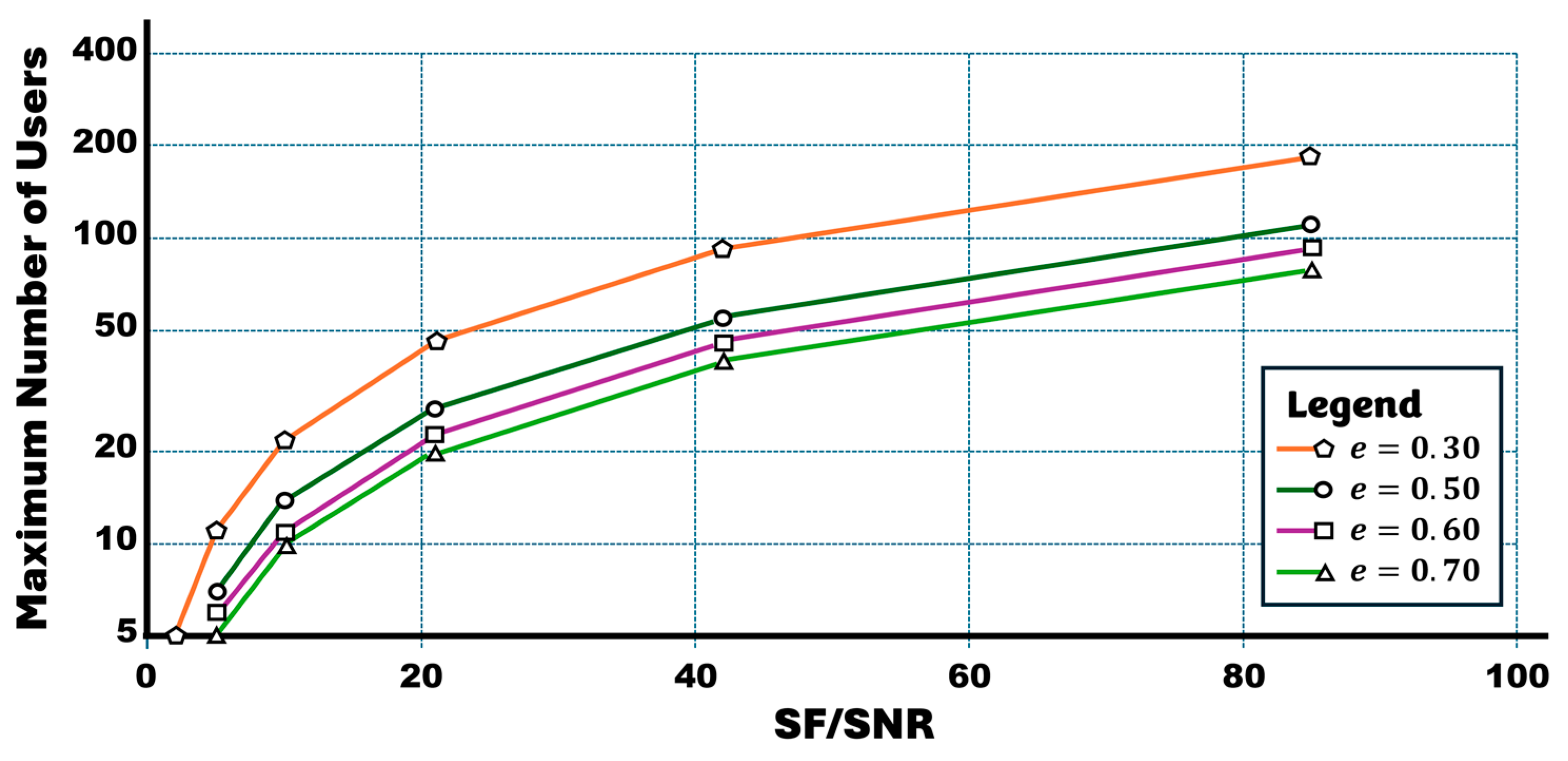
• This research study derives capacity bounds in various propagation scenarios while considering mobility scenarios and two crucial elements that affect performance: interference and restricted transmission power.
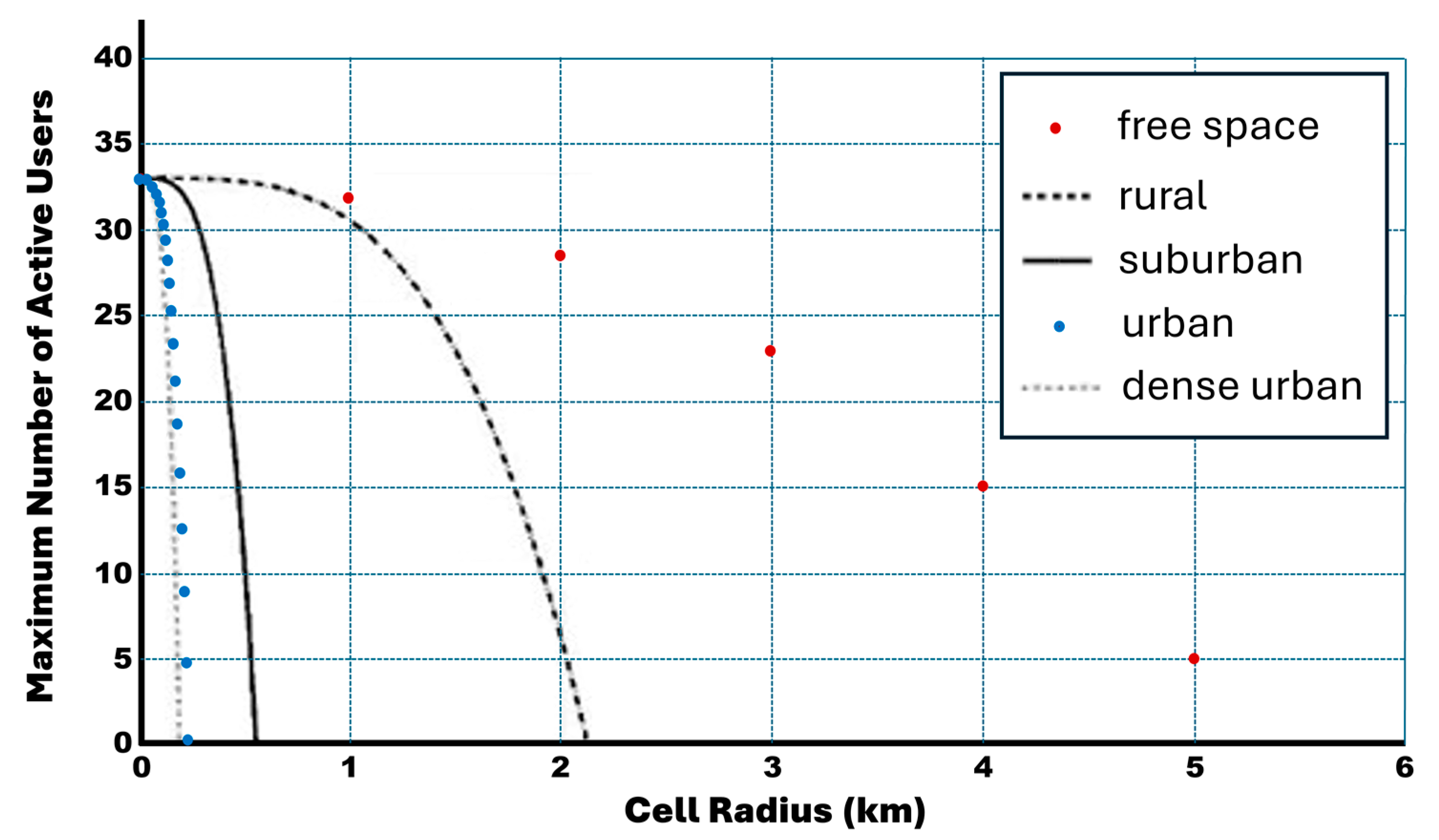
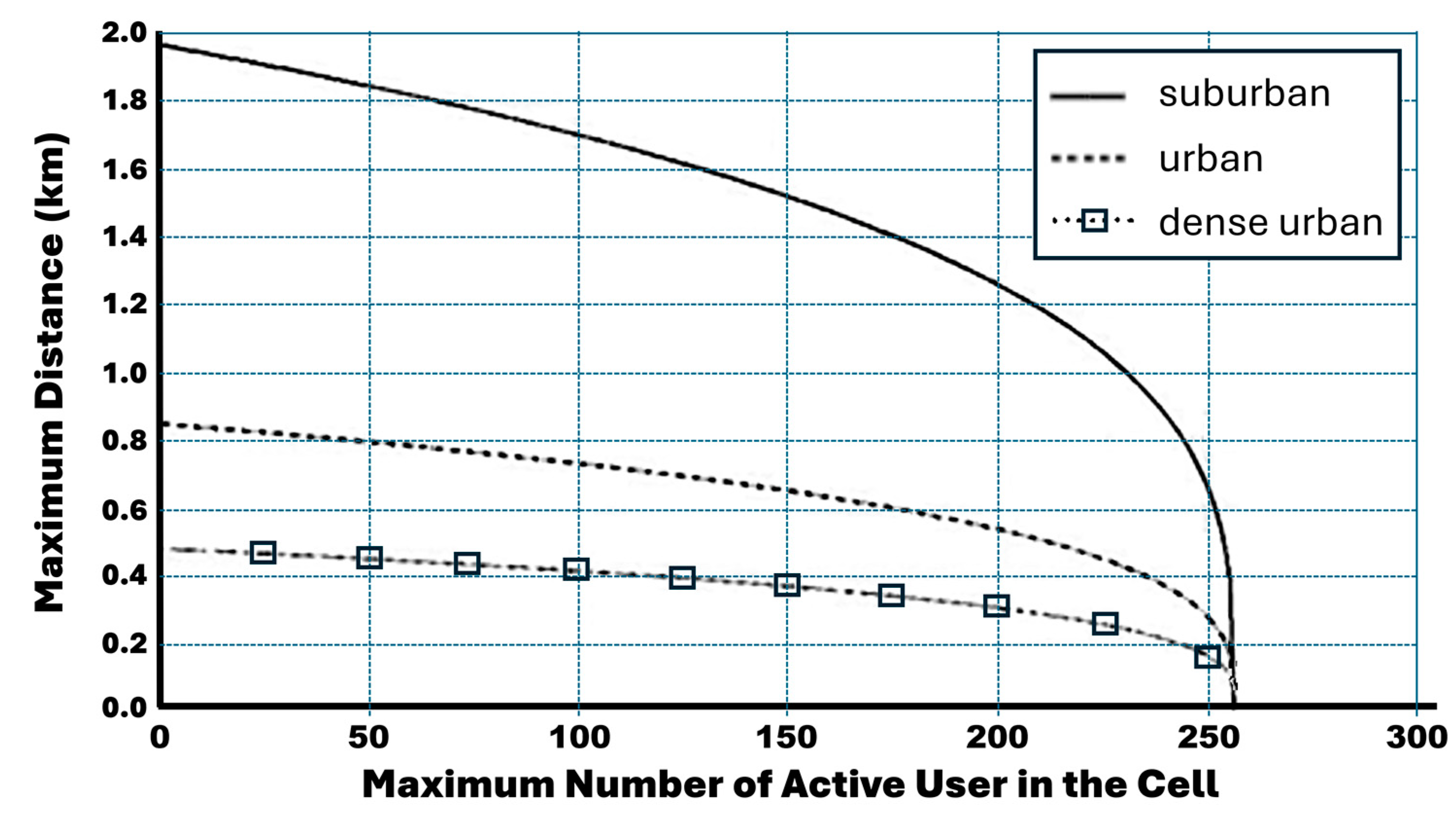
• Based on the multiservice case of the derived capacity bounds, new numerical results with a discussion and explanation of the new results are presented in this extended version, taking into consideration the cell breathing phenomenon, which affects cell coverage and capacity by considering different cell sizes.
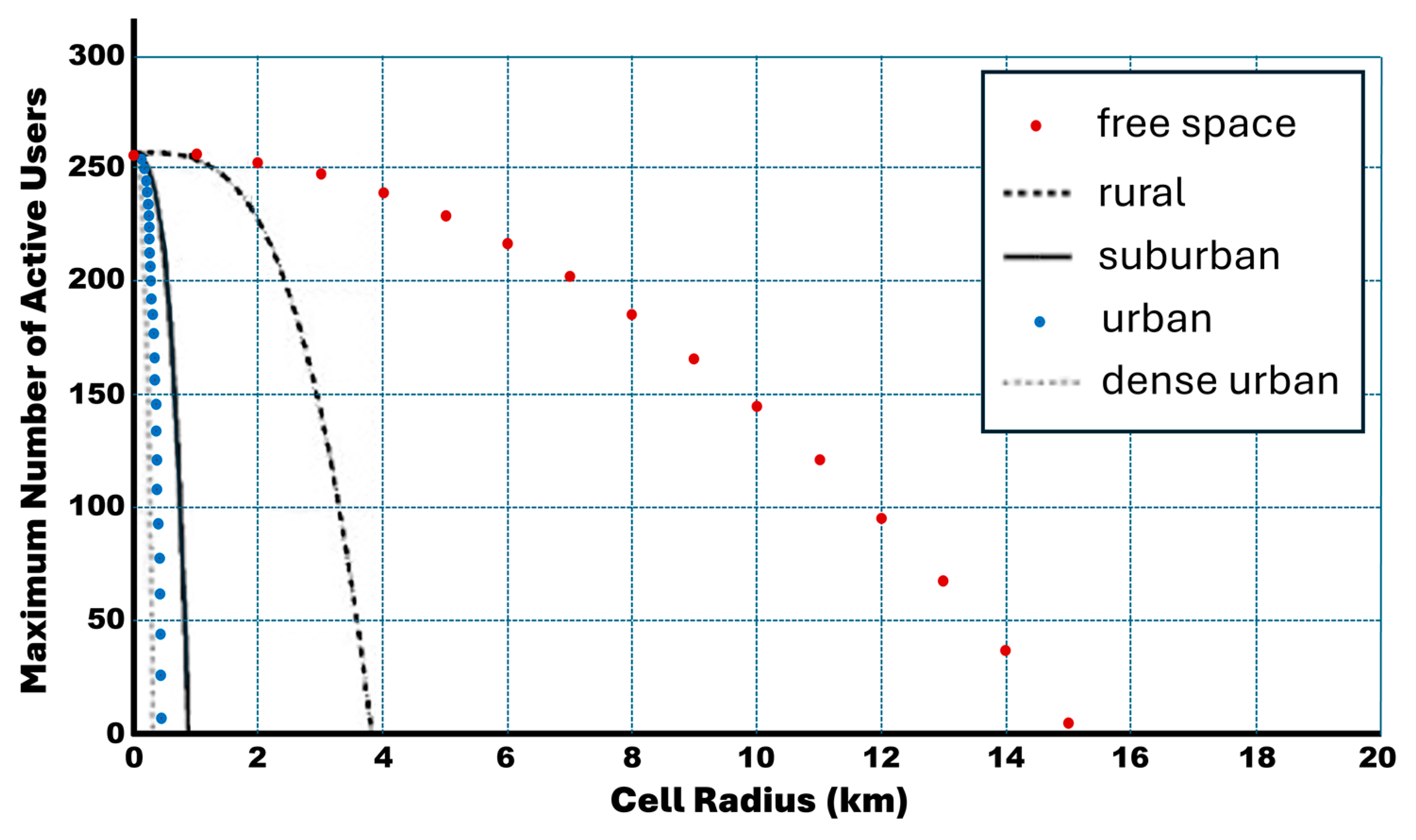
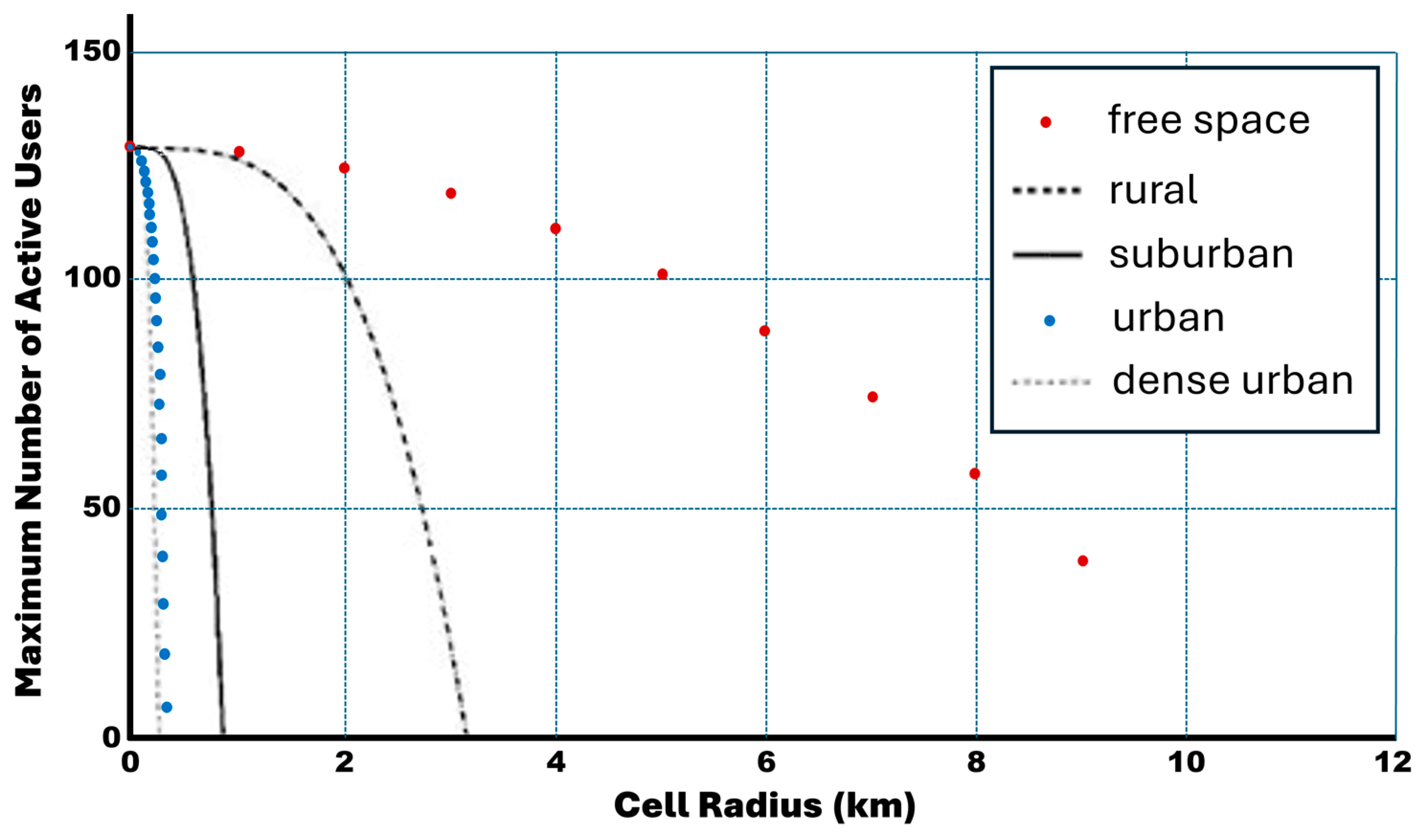
• Because performance analysis of the new generation of mobile networks will not be realistic considering only the free-space propagation model, the capacity bounds analysis in this research work, along with a comprehensive discussion through the numerical results, will provide a key indicator for mobile operators to be well thought out in the future planning of 5G networks.
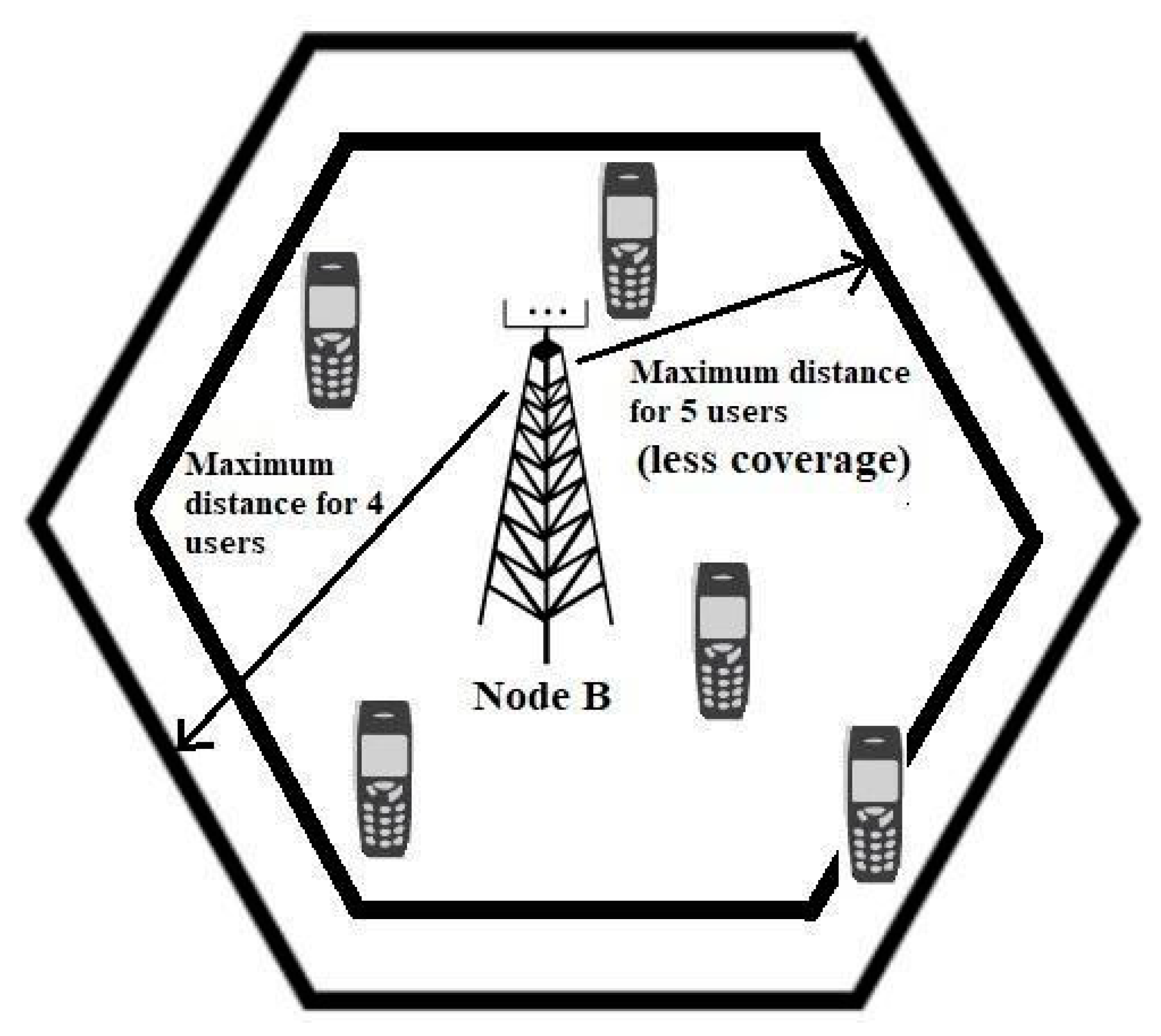
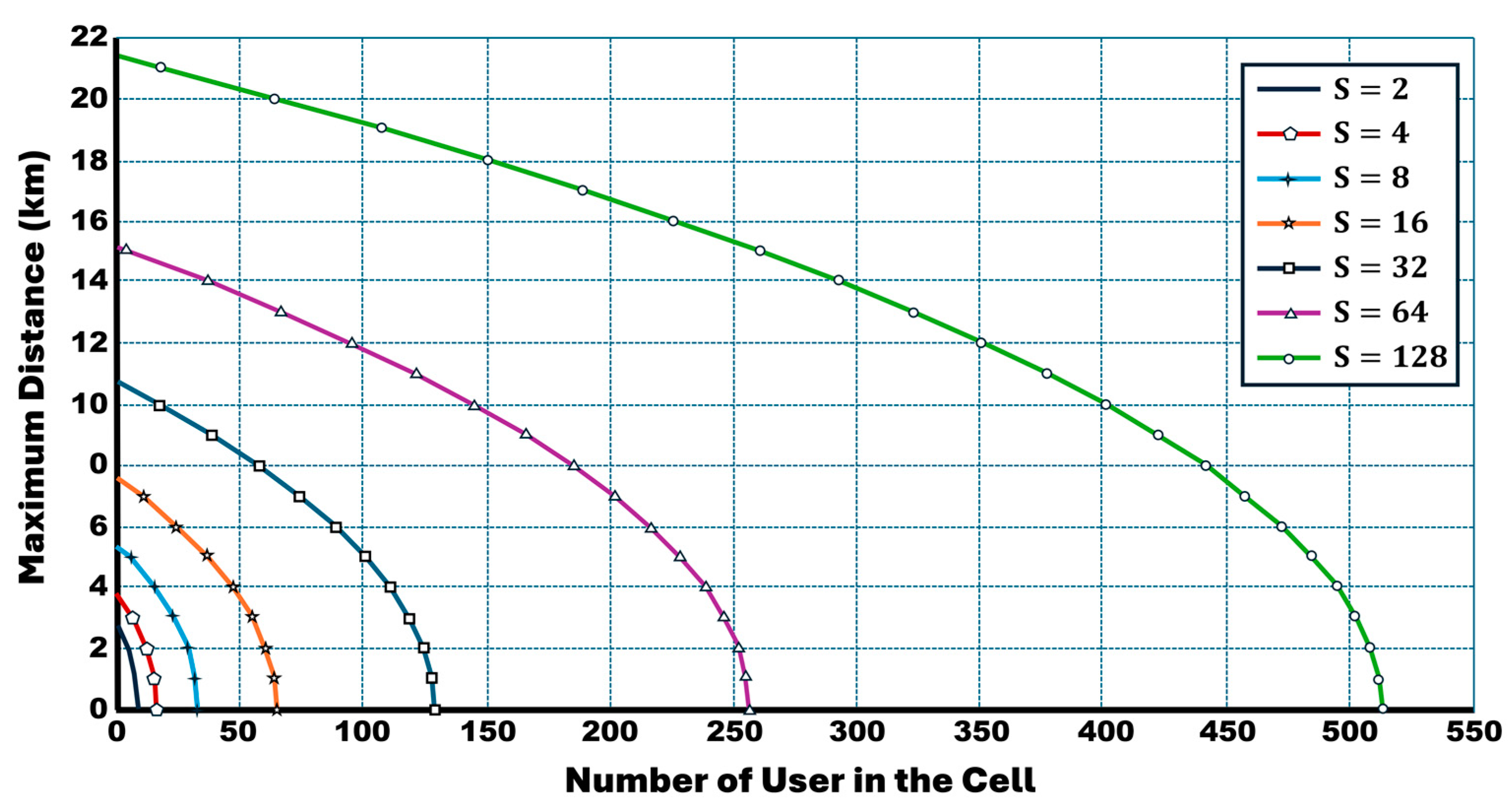
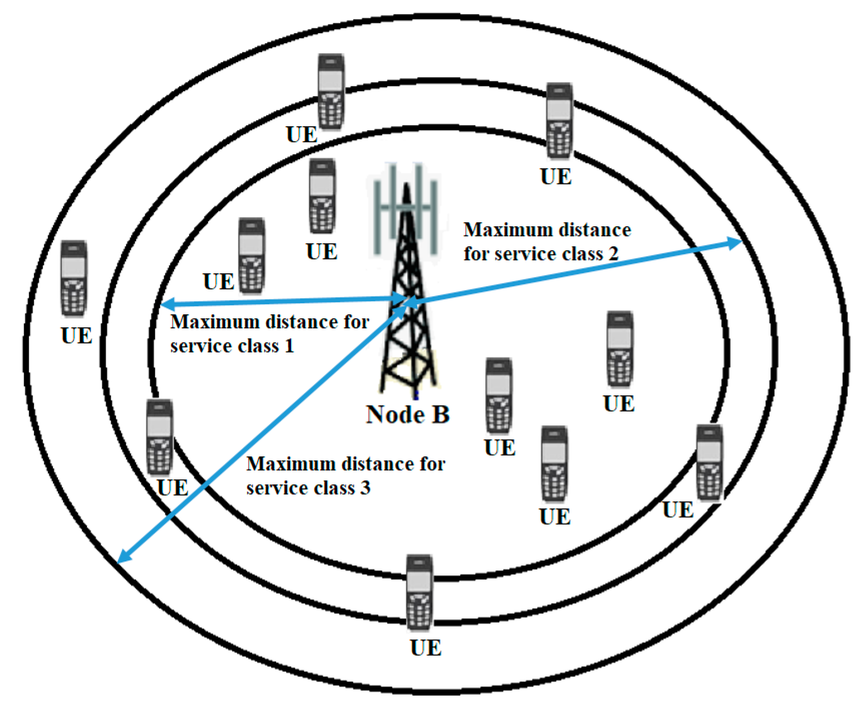
• The following new figures illustrate how the maximum distance and coverage change based on the selected service class.
• In addition, the following parts are changed, modified, or added:

  ○

  The Abstract and Conclusions have been changed.

  ○

  The Introduction and related work have been modified, and additional references have been added.

  ○

  The derivation of the capacity bounds in a multiservice case is given.

  ○

  A new group of results is added to reflect the effect of the multiservice case capacity bounds on cell coverage and capacity considering different service categories and mobility scenarios. Consequently, the “Simulation results and discussions” Section is changed to demonstrate this effect.

• The impacts of cell breathing, interference, and environment-specific path loss (via COST-231 Hata extensions) are quantified.
• Actionable insights for network planning (e.g., trade-offs between coverage and capacity) are provided.

The remainder of this paper is organized as follows. Section 2 includes related work. Section 3 overviews the extended COST-Hata model. The derivation and analysis of the capacity bounds are described in Section 4. In Section 5, 5G performance with multiservice is introduced. The simulation results and discussion are presented in Section 6. Section 7 concludes the paper by discussing future studies. Finally, a list of relevant references is provided. The framework diagram of this paper’s structure is given in Figure 1.

2. Related Work

Mobile operators face enormous challenges as a result of the recent transition from 4G to 5G systems, as users are switching from traditional applications to a new network design that supports a variety of applications that virtually connect machines, objects, and devices with multi-gigabit speed, negligible latency, and maximum spectrum efficiency. Studying the capacity bounds of these systems in more accurate scenarios can help us solve the aforementioned difficulties by more accurately reflecting the end-user experience. The literature examines and analyzes capacity bounds from various perspectives and angles.

In a previous study [19], Shannon’s capacity formula was used to calculate system capacity. The authors used long-term evolution (LTE) as a case study to forecast the LTE spectral efficiency in micro and macro contexts. The authors report a perfect match between the expected and simulated values based on the generated results. In [20], the authors used spectral constraints and quantization techniques to derive capacity boundaries. The authors concluded that although employing low quantization resolution does not affect the possible rates of 5G systems, satisfying out-of-band constraints is a barrier to the future of 5G systems. By employing finite block-length coding, the authors of [21] proposed QoS provisioning with a statistically constrained delay parameter for multimedia mobile wireless networks, such as 5G. The capacity formulation of such systems is influenced by delay-bounded QoS restrictions. The authors used simulation findings to validate the system performance results.

The capacity bound has been studied by authors in the recent literature [22,23,24,25,26,27,28] based on various criteria and viewpoints. The error probability and capacity constraints in [22] were calculated by the authors based on the unique modulation symbols of the vertical bell labs space–time system. The upper bound for the average bit error probability was derived by the authors, who also created a successful error correction system. Comparing the proposed detection with a compressive sampling–matching pursuit detector, the authors claimed that the proposed detection is much more practical for spatial modulation schemes. Time-varying channel characteristics and signal loss are the two fundamental issues faced by rail train carriages, and efficient capacity analysis and transceiver design were derived in [23] to address these issues. The authors assert that the recommended strategies perform better than conventional methods currently used to address these issues, such as relay and beamforming. With a suggestion for transceiver design, lower and upper bounds of capacity were established, and the simulation results showed that the prediction method can be very helpful for future channel predictions.

In contrast to other works in the literature, a device-to-device communication model was proposed in [24], according to the authors, assuming a nun-ideal transceiver with interference and no channel state information. Saddle-point approximations were used to derive the upper and lower capacity limitations in the closed form. The numerical results demonstrate that mmWave communication can resist transceiver noise even at high signal-to-noise ratios (SNRs). The capacity results were tested against a Monte Carlo simulation. The authors of [25] investigated the impact of remaining hardware deficiencies on the ergodic capacity of dual-hop (DH) amplify-and-forward (AF) MIMO relay systems by considering the beneficial effects of the MIMO relay model on the coverage and capacity of next-generation wireless networks. The authors used a simulation to examine the impact of low SNR values on the system capacity, in addition to determining the upper and lower limits of the capacity. According to the modeling results, the capacity reaches saturation when the transceiver degrades. The upper capacity limitations of the large intelligent surface (LIS) antenna were derived in [26]. The authors argue that locations with many LISs can attain maximum capacity using a greedy scheduling technique and Monte Carlo simulation. For urban regions, a new route loss model was proposed in [27] that considers novel characteristics, including window size, humidity, and temperature. In comparison with other models in the literature, the authors asserted that the proposed model increases the estimation of path loss by 10%.

A capacity study of device-to-device (D2D) communication over mmWave 5G cellular networks was introduced in [28], taking into account real constraints such as transceiver distortion noise, channel state information (CSI), and interference from neighboring cells. Based on the numerical results, the authors concluded that transceiver distortion noise has a significant impact on the performance of future communication systems, particularly at high SNRs. In addition, the performance of such systems is compromised by the addition of more disruptive nodes to the network.

To achieve the aim of maximizing sum spectrum efficiency, the authors in [29] have proposed a joint interference suppression scheme in heterogeneous networks with dense small cells and users considering co-tier intra-cell interference alignment. Due to the exponential growth of the output layer neurons faced by general deep reinforcement learning algorithms, the authors proposed a deep deterministic policy gradient-based algorithm to solve the problem. As per the provided numerical results, the authors claimed that the proposed algorithm is able to achieve better performance and wider application scope compared with existing algorithms. On the other hand, article [30] examines computational offloading in networks beyond 5G in response to the trend of combining wireless communications and multi-access edge computing. A distributed learning framework is proposed in order to overcome the technical difficulties arising from the uncertainties and the sharing of restricted resources in multi-access edge computing systems. Moreover, and in order to demonstrate the possibilities of an online distributed reinforcement learning algorithm created using the suggested architecture, the authors provided a case study on resource orchestration in computation offloading. As per the provided comparative experimental results, the authors show that the suggested learning method algorithm works better than the benchmark resource orchestration algorithms.

3. The Extended COST-231 Hata Model

In contrast to COST-231 Hata, the expanded version of the empirical model proposes a general path propagation equation to replace the signal intensity caused by path loss and to span a wider frequency range. The general free-space model [31] encompasses two terms: a logarithm part based on distance and another logarithm part based on frequency, as shown below:

$${PL}_E\left(d\right)={PL}_E\left(d\right)=32.44+20\log \left(f\right)+20\log \left(d\right)$$

(1)

Here, $E$ is zero for a free space model according to the assumed code given in

Table 1. Codes assumed for each environment.

$\mathbf{Environment} \mathbf{Type} \left(\mathit{E}\right)$	Code
Free Space	$0$
Urban	$1$
Suburban	$2$
Dense Urban	$3$
Rural	$4$

for each type of environment E.

However, the propagation loss equations are derived in this study for different realistic environments, such as dense urban, urban, suburban, and rural environments, based on the propagation equation given in [32] as follows:

$$\begin{gathered} {PL}_E={PL}_E\left(d\right)=46.3+33.9\log \left(f\right)-13.82\log \left(h_b\right)-a\left(h_m\right) \\ +\left(44.9-6.55\log \left(h_b\right)\right)\log \left(d\right)+{CF}_E \end{gathered}$$

(2)

Notations. We introduce ${CF}_E$ as a correction factor for each environment type $E$. ${PL}_E$ is the path loss for environment type $E$ in dB, as assumed in Table 1. $f$ is the frequency in MHz. $h_b$ is the height of the base station or transmitter in meters, $m$. $h_m$ is the height of the mobile or receiver in meters. $d$ is the distance between the transmitter and receiver in kilometers, Km. $a\left(h_m\right)$ is the correction factor of the mobile antenna.

Note that in (2), the propagation loss equation differs in each environment concerning two parameters, namely $a\left(h_m\right)$ and${CF}_E$.

Therefore, the propagation loss equations [32] are derived using (2) to obtain the following:

1.

The propagation model for an urban environment is as follows:

$${PL}_1=46.3+33.9\log \left(f\right)-13.82\log \left(h_b\right)-a\left(h_m\right)+\left(44.9-6.55\log \left(h_b\right)\right)\log \left(d\right)$$

(3)

where

$$a\left(h_m\right)=\left(1.1\log \left(f\right)-0.7\right)h_m-\left(1.56\log \left(f\right)-0.8\right) \mathrm{d}\mathrm{B}$$

2.

The propagation model for the suburban environment is as follows:

$${PL}_2={PL}_1-2{\left(\log \left(f\right)-\log 28\right)}^2-5.4$$

(4)

3.

The propagation model for the dense urban environment is as follows:

$$\begin{gathered} {PL}_3=46.3+33.9\log \left(f\right)-13.82\log \left(h_b\right)-a\left(h_m\right) \\ +\left(44.9-6.55\log \left(h_b\right)\right)\log \left(d\right)+3 \end{gathered}$$

(5)

where

$$a\left(h_m\right)=3.2{\left(\log \left(11.75·h_m\right)\right)}^2-4.97 \mathrm{d}\mathrm{B}$$

4.

The propagation model for a rural environment is as follows:

$${PL}_4={PL}_1-4.78{\left(\log \left(f\right)\right)}^2+18.33\log \left(f\right)-40.94$$

(6)

4. Capacity Bounds Analysis

4.1. Single-Service Capacity Bounds

4.1.1. Capacity Bounds Due to the Interference

It is well known that any user actively using a cell can cause interference with other users. User i should boost power as required to meet the node requirements when more users become active. We consider a single-service case. Since all users achieve the required SNRi (Si = SFi/SNRi = S), it is presumed that all users transmit a signal with the same spreading factor, SFi. Additionally, for all code combinations, the non-orthogonality factor, ε_ij, will be equal. Every active user in the cell causes some interference for the other users. A user’s interference level increases with the number of users entering the cell; hence, this user needs to supply more transmission power. If the number of users in the cell reaches a certain limit, the system can no longer increase the received power to improve the signal-to-noise ratio (SNR) because of the linear relationship between the received power $P_R$ of user i and the resulting interference level of all the other users. This limit is indicated by the following condition:

$$S>(n-1)·{\displaystyle \frac{V\cdot \epsilon }{F}}$$

Given the derivation of$P_R$ in [32] and assuming that all users in the cell are using the same radio service and that n users are interfering with each other in the cell, thermal noise,${ N}_0$, is generated in the cell and is derived as follows:

$$N_0=P_R\left(S-(n-1)·{\displaystyle \frac{V\cdot \epsilon }{F}}\right)$$

(7)

Because of the linear relationship between the received power of user $i$, ${PP}_i$, and the interference caused by other users in the cell, the system cannot improve the signal-to-noise ratio (SNR) when the number of active users, $n_{max}$, reaches a specific limit. Therefore, from (7), we obtain the following:

$$n_{\mathrm{m}\mathrm{a}\mathrm{x}}<{\displaystyle \frac{S·F}{V·\epsilon }}+1$$

(8)

Notations. $n_{\mathrm{m}\mathrm{a}\mathrm{x}}$ is the maximum number of active users in the cell, $\epsilon$ is the non-orthogonality factor of the user’s signals, S is the service factor (S = SF/SNR), and SF is the spreading factor representing the number of chips per data symbol. Here, V is the activity factor for any type of user service, and F is the inter-cell interference factor.

4.1.2. Capacity Bounds Due to Limited Uplink Transmission Power

The maximum transmitted power $P_{\mathrm{S}\mathrm{m}\mathrm{a}\mathrm{x}}$ of the user equipment (UE) depends on the distance d between the UE and Node B. Therefore, the UE may not be able to achieve the desired received power, $P_R$, at Node B due to path loss. Because of this fact, the following is very well known [19]:

$$P_R=P_{\mathrm{S}\mathrm{m}\mathrm{a}\mathrm{x}}·{PL}_E\left(d_{\mathrm{m}\mathrm{a}\mathrm{x}}\right)$$

(9)

Notations. $P_R$ is the power received at Node B, $P_{\mathrm{S}\mathrm{m}\mathrm{a}\mathrm{x}}$ is the maximum power sent by the UE, ${PL}_E\left(d_{\mathrm{m}\mathrm{a}\mathrm{x}}\right)$ is the path that depends on the distance between the UE and Node B, and parameter E is the code to be used for the type of environment (free space, urban, dense-urban, suburban, and rural).

However, in a real environment, the power budget may not be perfect. Therefore, the power control error $P_{\mathrm{e}\mathrm{r}\mathrm{r}}$ should be considered in the path loss as a substitute for the difference between the real and estimated path losses due to fading. Consequently, (9) can be written as follows:

$$P_R=P_{\mathrm{S}\mathrm{m}\mathrm{a}\mathrm{x}}·{PL}_E\left(d_{\mathrm{m}\mathrm{a}\mathrm{x}}\right)\cdot P_{\mathrm{e}\mathrm{r}\mathrm{r}}$$

(10)

Then,

$${PL}_E\left(d_{\mathrm{m}\mathrm{a}\mathrm{x}}\right)={\displaystyle \frac{P_R}{P_{\mathrm{S}\mathrm{m}\mathrm{a}\mathrm{x}}\cdot P_{\mathrm{e}\mathrm{r}\mathrm{r}}}}$$

(11)

By substituting the value of $P_R$ in (7) into (11), we obtain the following:

$${PL}_E\left(d_{\mathrm{m}\mathrm{a}\mathrm{x}}\right)={\displaystyle \frac{N_0}{\left(S-(n-1)·\frac{V\cdot \epsilon }{F}\right)\cdot P_{\mathrm{S}\mathrm{m}\mathrm{a}\mathrm{x}}\cdot P_{\mathrm{e}\mathrm{r}\mathrm{r}}}}$$

(12)

Recalling [19,20], the path loss of free space propagation is expressed as follows:

$${\displaystyle \frac{P_R}{P_{\mathrm{S}\mathrm{m}\mathrm{a}\mathrm{x}}}}={\left({\displaystyle \frac{\lambda }{4\pi \cdot d_{\mathrm{m}\mathrm{a}\mathrm{x}}}}\right)}^2\cdot g_b\cdot g_m={PL}_E\left(d_{\mathrm{m}\mathrm{a}\mathrm{x}}\right)$$

(13)

Substituting the ${PL}_E\left(d_{max}\right)$ value from (12) into (13) gives $P_R$ being dependent on the number of active users in a single-cell case; thus, the antenna gains $g_b$, $g_m$, and $P_{\mathrm{e}\mathrm{r}\mathrm{r}}$ are all assumed to be 1. We obtain

$${\left({\displaystyle \frac{\lambda }{4\pi \cdot d_{\mathrm{m}\mathrm{a}\mathrm{x}}}}\right)}^2={\displaystyle \frac{N_0}{\left(S-(n-1)·\frac{V\cdot \epsilon }{F}\right)\cdot P_{\mathrm{S}\mathrm{m}\mathrm{a}\mathrm{x}}}}$$

(14)

Notations. $\lambda$ is the wavelength $\lambda =c/f$ ($c$ is the speed of light and $f$ is the frequency), and $d_{\mathrm{m}\mathrm{a}\mathrm{x}}$ is the maximum distance between the UE and Node B.

For a single-service example, the number of active users in the cell, $n$, determines the received power,$PR$. When the load on the cell increases, the cell’s effective coverage decreases because an additional user causes more interference for existing users, according to the cell breathing phenomena [17,21] shown in Figure 2. As a result, people who are near cell borders have the best chance of being in adjacent cells.

From (14) and based on the derivation in [12], the new formula for $d_{\mathrm{m}\mathrm{a}\mathrm{x}}$ as a function of $n$ can be expressed as follows:

$$d_{\mathrm{m}\mathrm{a}\mathrm{x}}\left(n\right)={\displaystyle \frac{\lambda }{4\pi }}\cdot \sqrt{{\displaystyle \frac{P_{\mathrm{S}\mathrm{m}\mathrm{a}\mathrm{x}}\cdot {PL}_E\left(d\right)}{N_0}}\cdot \left(S-(n-1)·{\displaystyle \frac{V\cdot \epsilon }{F}}\right)}$$

(15)

Mobile operators should consider the coverage of a particular cell because the maximum number of active users in a cell varies dynamically. As a result, it is crucial to consider cell planning for users who are actively depending on cell coverage and the existing radio link service.

Figure 2. Cell breathing.

Figure 2. Cell breathing.

Therefore, from (14), the maximum number of active users, $n_{\mathrm{m}\mathrm{a}\mathrm{x}}$, can be reformulated as follows, where $n$ is replaced with $n_{\mathrm{m}\mathrm{a}\mathrm{x}}$:

$$\left(S-{\displaystyle \frac{{\left(4\pi \cdot d_{\mathrm{m}\mathrm{a}\mathrm{x}}\right)}^2\cdot N_0}{P_{\mathrm{S}\mathrm{m}\mathrm{a}\mathrm{x}}\cdot {\lambda }^2}}\right)·{\displaystyle \frac{F}{V\cdot \epsilon }}=n_{\mathrm{m}\mathrm{a}\mathrm{x}}-1$$

(16)

Afterward, move $n_{\mathrm{m}\mathrm{a}\mathrm{x}}$ to the left to obtain

$$n_{\mathrm{m}\mathrm{a}\mathrm{x}}=\left(S-{\displaystyle \frac{{\left(4\pi \cdot d_{\mathrm{m}\mathrm{a}\mathrm{x}}\right)}^2\cdot N_0}{P_{\mathrm{S}\mathrm{m}\mathrm{a}\mathrm{x}}\cdot {\lambda }^2}}\right)·{\displaystyle \frac{F}{V\cdot \epsilon }}+1$$

(17)

The maximum number of active users in the cell can also be represented by rewriting (17) as follows, presuming that the cell has an ideal circle with a radius, $r$.

$$n_{\mathrm{m}\mathrm{a}\mathrm{x}}=\left(S-{\displaystyle \frac{{\left(4\pi \cdot r\right)}^2\cdot N_0}{P_{\mathrm{S}\mathrm{m}\mathrm{a}\mathrm{x}}\cdot {\lambda }^2}}\right)·{\displaystyle \frac{F}{V\cdot \epsilon }}+1$$

(18)

4.2. Multiservice Capacity Bounds

Unlike a single-service case, in a multiservice case, different radio link services, $k$, will be requested by the user, and different spreading factors, ${SF}_i$, different signal-to-noise ratios, ${SNR}_i$, and therefore different service factors, ${Sk}_i$ parameters, will be requested by the user.

A simplified calculation model is suggested in this analysis, which is based on the following assumptions:

• $n_k$ is the number of active users requiring the same radio service ($k$) with identical service factor values, $S_k$.
• The non-orthogonality factor, ${\epsilon }_{ij}$, is equal for different user signals $i$ and $j$ using the same service factor, $S_k$.
• The inter-class interference between users due to the non-orthogonality of the codes for a single-service type $k$ is assumed to be ${\epsilon }_k$. In contrast, the inter-class interference factor, ${\epsilon }_k$, is between all users $i$ of service $l$, and all users $j$ of service $k$ are assumed to be the same.
• The received power, $P_{Ri}$, required at node B is assumed to be the same for all user signals using the same service, $S_k$. In this case, the received power at node B is denoted by $P_{Rk}$.

Similarly to previous generations of mobile networks, in 4G networks, the power budget of the uplink differs from that of the downlink. The uplink power budget is based on the transmitted signal of the UE, whereas in the downlink, it is based on the capability of Node B. Considering the uplink power budget, each user transmits a signal with a given transmitted power, $P_S$, calculated by the UE, to Node B with less power due to path loss. Consider applying the coding principle at Node B; the user’s signals generate noise due to the non-orthogonality of the codes, which is referred to as the non-orthogonality factor${\epsilon }_{ij}$. In other words, the interference $I_i$ observed at Node B for user $i$ signal is the sum of the received power of all other users $j$ multiplied by the non-orthogonality factor${\epsilon }_{ij}$. The interference $I_i$ observed at Node B for user $i$ signal is the sum of the received power of all the other users $j$ multiplied by the non-orthogonality factor. In this case, there is thermal noise, $N_t$, and the interference from the neighboring cells, $\mathsf{\chi }\left(\mathit{n}\right)$ where $\mathit{n}=\left(n_2,\dots ,{ n}_m\right)$ is the number of active users in the neighboring cells. Therefore, interference $I_i$ can be reformulated as follows:

$$I_i=N_t+\chi \left(\mathit{n}\right)+\sum _{j=1, j\ne i}^{n_1}{V}_j\cdot P_{Rj}\cdot {\epsilon }_{ij}$$

(19)

In Equation (19), the activity factor, $V_j$, for user $j$, which depends on the type of service user $j$ requests, is introduced. It is also called the service activity factor. Service activity means the continuous use of some service in a cell. Monitoring voice/data activity in a cell is an important technique to reduce interference or to increase the capacity as each transmitter is switched off during the period of no activity, and these periods can be used for other data flow without losing the quality of service (QoS). Based on the spreading technique, the data symbol of a given user spreads on a certain number of chips; therefore, the spreading factor, ${SF}_i$, is defined as the number of chips on which the data symbol spreads, creating something called the spreading gain of the signal. The more chips the signal spreads on, the higher the spreading gain, but the lower the symbol data rate is. Considering this principle, the received signal power of user $i$ after dispreading is expressed as follows:

$$C_i={SF}_i\cdot P_{Ri}$$

(20)

After decoding the signal at Node B, given the required bit error ratio (BER), a certain signal-to-noise ratio (SNR, i.e., $E_b/N_0$) should be satisfied for each user signal to guarantee the required quality of service (QoS). The SNR value is service-dependent on the modulation technique, BER, and the forward error correction scheme considered. Therefore, the SNR can be considered as the ratio of received power after dispreading and the interference caused by other users’ signals and can be expressed as follows:

$${\displaystyle \frac{C_i}{I_i}}$$

(21)

From (19)–(21), the following relation is considered:

$${\displaystyle \frac{C_i}{I_i}}={\displaystyle \frac{{SF}_i\cdot P_{Ri}}{N_t+\chi \left(\mathit{n}\right)+\sum _{j=1, j\ne i}^{n_1}{V}_j\cdot P_{Rj}\cdot {\epsilon }_{ij}}}\ge {\left({\displaystyle \frac{E_b}{N_0}}\right)}_i$$

(22)

If there are $n_1$ active users in a given cell, (22) can be written as follows:

$${\left({\displaystyle \frac{E_b}{N_0}}\right)}_i={\displaystyle \frac{{SF}_i\cdot P_{Ri}}{N_t+\chi \left(\mathit{n}\right)+\sum _{j=1, j\ne i}^{n_1}{V}_j\cdot P_{Rj}\cdot {\epsilon }_{ij}}}\ge {\left({\displaystyle \frac{E_b}{N_0}}\right)}_i$$

(23)

For $i$ and $j$, they are from $1,\dots ,n_1$

The service factor S can be defined as follows:

$$S_i={\displaystyle \frac{{SF}_{i }}{{\left(\frac{E_b}{N_0}\right)}_i }}$$

(24)

we also introduce the ratio of the interference from other cells (i.e., inter-cell interference) to the interference of the visiting cell (intra-cell interference) as follows [31,32,33]:

$$IR\left(n\right)={\displaystyle \frac{\mathrm{i}\mathrm{n}\mathrm{t}\mathrm{e}\mathrm{r}-\mathrm{c}\mathrm{e}\mathrm{l}\mathrm{l} \mathrm{i}\mathrm{n}\mathrm{f}\mathrm{t}\mathrm{e}\mathrm{r}\mathrm{f}\mathrm{e}\mathrm{r}\mathrm{e}\mathrm{n}\mathrm{c}\mathrm{e}}{\mathrm{i}\mathrm{n}\mathrm{t}\mathrm{r}\mathrm{a}-\mathrm{c}\mathrm{e}\mathrm{l}\mathrm{l} \mathrm{i}\mathrm{n}\mathrm{f}\mathrm{t}\mathrm{e}\mathrm{r}\mathrm{f}\mathrm{e}\mathrm{r}\mathrm{e}\mathrm{n}\mathrm{c}\mathrm{e}}}={\displaystyle \frac{\chi \left(\mathit{n}\right)}{\phi \left(n_1\right)}}$$

(25)

where $\phi \left(n_1\right)={\sum }_{k=1}^{n_k-1}{V}_{k }·{{\epsilon }_{ij}·P}_{Rj}$ is for single-service case and $\mathit{n}=\left(n_2,\dots ,n_m\right)$ is the number of connections among all neighboring cells, and $m$ is the number of neighboring cells. The inter-cell interference factor $F$ is defined [34,35] as

$$F={\displaystyle \frac{1}{IR+1}}$$

(26)

Equation (25) can be rewritten as follows:

$$\chi \left(\mathit{n}\right)=IR\left(n\right)\cdot \phi \left(n_1\right)$$

(27)

By substituting $\mathsf{\chi }\left(\mathit{n}\right)$ of (27) and $\phi \left(n_1\right)$ of (25) into (23), we obtain the following:

$${\left({\displaystyle \frac{E_b}{N_0}}\right)}_i={\displaystyle \frac{{SF}_i\cdot P_{Ri}}{N_t+IR\left(n\right)\cdot \phi \left(n_1\right)+\phi \left(n_1\right)}}$$

(28)

To simplify the derivation, we consider $n_1=n$, and (28) can be rewritten as follows:

$$N_t+\left(IR+1\right)\cdot \phi \left(n\right)=S_i\cdot P_{Ri}$$

(29)

By substituting the value of $\phi \left(n\right)$ from (25) into (29), we obtain the following:

$$N_t=S_i\cdot P_{Ri}-\left(IR+1\right)\cdot \sum _{k=1}^{n_k-1}{V}_{k }·P_{Rj}·{\epsilon }_{ij}$$

(30)

Using matrix notation, the power conditions for all user signals arriving at Node B can be expressed as follows:

$$\mathbf{N}=\left(\mathbf{S}-\left(IR+1\right)\cdot \mathbf{V}\cdot \mathbf{E}\right)\cdot {\mathbf{P}}_{\mathbf{R}}$$

(31)

where

$\mathbf{N}={\left(N_t\dots N_t\right)}^T$ is a noise vector of dimension $n$;

$\mathbf{S}=\mathrm{d}\mathrm{i}\mathrm{a}\mathrm{g}\left(S_1\dots S_n\right)$ is a diagonal matrix of dimension $\left(n\times n\right)$;

${\mathbf{P}}_{\mathbf{R}}={\left(P_{R1}\dots P_{Rn}\right)}^T$ is the power vector;

$\mathbf{V}=\mathrm{d}\mathrm{i}\mathrm{a}\mathrm{g}\left(V_1\dots V_n\right)$ is the service activity factor;

$\mathbf{E}$ is the non-orthogonality factor in the following structure:

$$\mathbf{E}=\left[\begin{array}{cccc}0& {\epsilon }_{12}& \cdots & {\epsilon }_{1n}\\ {\epsilon }_{21}& 0& \cdots & {\epsilon }_{2n}\\ ⋮& ⋮& \ddots & ⋮\\ {\epsilon }_{n1}& {\epsilon }_{n2}& \cdots & 0\end{array}\right]$$

(32)

Solving the above linear system of equations, user $i$ can obtain the received power at Node B.

By (25), the intra-cell interference for a user of class k can be redefined in a multiservice case as follows:

$${\phi }_k\left(\mathit{n}\right)=\sum _{m=1}^{n_k-1}{V}_{k }·{\epsilon }_k·P_{Rk}+\sum _{l\ne k, l=1}^s\sum _{i=1}^{n_l}{V}_{l }·{\epsilon }_{lk}·P_{Rl}$$

(33)

Equation (33) can be simplified as follows:

$${\phi }_k\left(\mathit{n}\right)=\left(n_k-1\right)V_{k }·{\epsilon }_k·P_{Rk}+\sum _{l\ne k, l=1}^s{n}_l\cdot V_{l }·{\epsilon }_{lk}·P_{Rl}$$

(34)

for $k$, $l=1\dots s$, where

$\mathit{n}=\left(n_1, n_2,\dots ,n_s\right)$;

$s$ represents several different service classes;

${\epsilon }_k$ is the interference factor between users in the same type of service $k$ (i.e., intra-class interference factor).

${\epsilon }_{lk}$ is the interference factor between user $i$ in service $l$ and user $j$ in service $k$ (i.e., inter-class interference factor).

$n_1$ is the number of connections of service type $l$.

$n_k$ is the number of connections of type $k$.

$V_l$ is the activity factor of service type $l$.

$V_k$ is the activity factor of service type $k$.

By substituting the value of $\phi$ of (34) into (28), and considering factor F in (26), we obtain the following:

$${\left({\displaystyle \frac{E_b}{N_0}}\right)}_k={\displaystyle \frac{{SF}_k·P_{Rk}}{N_t+\frac{1}{F}\left[\left(n_k-1\right)V_{k }·{\epsilon }_k·P_{Rk}+\sum _{l\ne k, l=1}^s{n}_l\cdot V_{l }·{\epsilon }_{lk}·P_{Rl}\right]}}$$

(35)

By the definition of $S_i$ given by (24), (35) can be rewritten as follows:

$$S_k\cdot P_{Rk}=N_t+{\displaystyle \frac{1}{F}}\left[\left(n_k-1\right)V_{k }·{\epsilon }_k·P_{Rk}+\sum _{l\ne k, l=1}^s{n}_l\cdot V_{l }·{\epsilon }_{lk}·P_{Rl}\right]$$

(36)

This can be further rewritten as follows:

$$N_t=S_k\cdot P_{Rk}-{\displaystyle \frac{1}{F}}\left[\left(n_k-1\right)V_{k }·{\epsilon }_k·P_{Rk}+\sum _{l\ne k, l=1}^s{n}_l\cdot V_{l }·{\epsilon }_{lk}·P_{Rl}\right]$$

(37)

4.2.1. Capacity Bounds Due to Interference

The number of active users in any given cell is interference-limited, and the maximum number of active users is primarily influenced by the non-orthogonality factor, $\epsilon$, as well as the requested service classes. Therefore, from (37) for any service class, the capacity bounds $k$ are limited as follows:

$$S_k\le {\displaystyle \frac{1}{F}}\cdot \left[-V_{k }·{\epsilon }_k+\sum _{l\ne k, l=1}^s{n}_l\cdot V_{l }·{\epsilon }_{lk}\right]$$

(38)

4.2.2. Capacity Bounds Due to Limited Uplink Power

The capacity bounds are limited by the maximum transmission power, ${PS}_{\mathrm{m}\mathrm{a}\mathrm{x}}$. Therefore, the maximum distance between the UE and Node B for a given service class, $k$, is expressed using (15) and (38), as follows:

$$d_{\mathrm{m}\mathrm{a}\mathrm{x}}\left(n_k,\mathit{n}\right)={\displaystyle \frac{\lambda }{4\cdot \pi }}\cdot \sqrt{{\displaystyle \frac{P_{\mathrm{S}\mathrm{m}\mathrm{a}\mathrm{x}}\cdot {PL}_E\left(d\right)}{N_t}}\left(S_{k }-{\displaystyle \frac{1}{F}}·\left(n_k-1\right)V_{k }·{\epsilon }_k-{\displaystyle \frac{1}{F}}\sum _{l\ne k, l=1}^s{n}_l·V_{l }·{\epsilon }_{lk}\right)}$$

(39)

where $\mathit{n}=\left\{n_l\right\}$, $l=1\cdots s$, $l\ne k$.

Because the received power, $P_{Rk}$, has a different value for each service factor, $S_k$, the maximum distance is changed based on the selected service class, as shown in Figure 3.

5. Fifth-Generation Performance with Multiservice

In wireless mobile networks, the service area is divided into cells with many available channels. There are two types of call requests that share these channels: new calls and handover calls. New calls are initiated by mobile users in the current cell, whereas handover calls are initiated in other cells and handed over to the current cell. When a call arrives at a cell in which a channel is not available, the call is blocked or queued, depending on the call admission control algorithm. The probability of a new call being blocked is called the new call-blocking probability, and the probability of a handover call being blocked is called the handover call probability. The probability that a call is either blocked or terminated during the call life is called the dropping probability. These probabilities are referred to as QoS metrics. In the following subsections, the performance of a 5G cell is studied in a multiservice case based on the above-derived capacity bounds.

5.1. Modeling Assumptions

The following modeling assumptions were considered in the analysis:

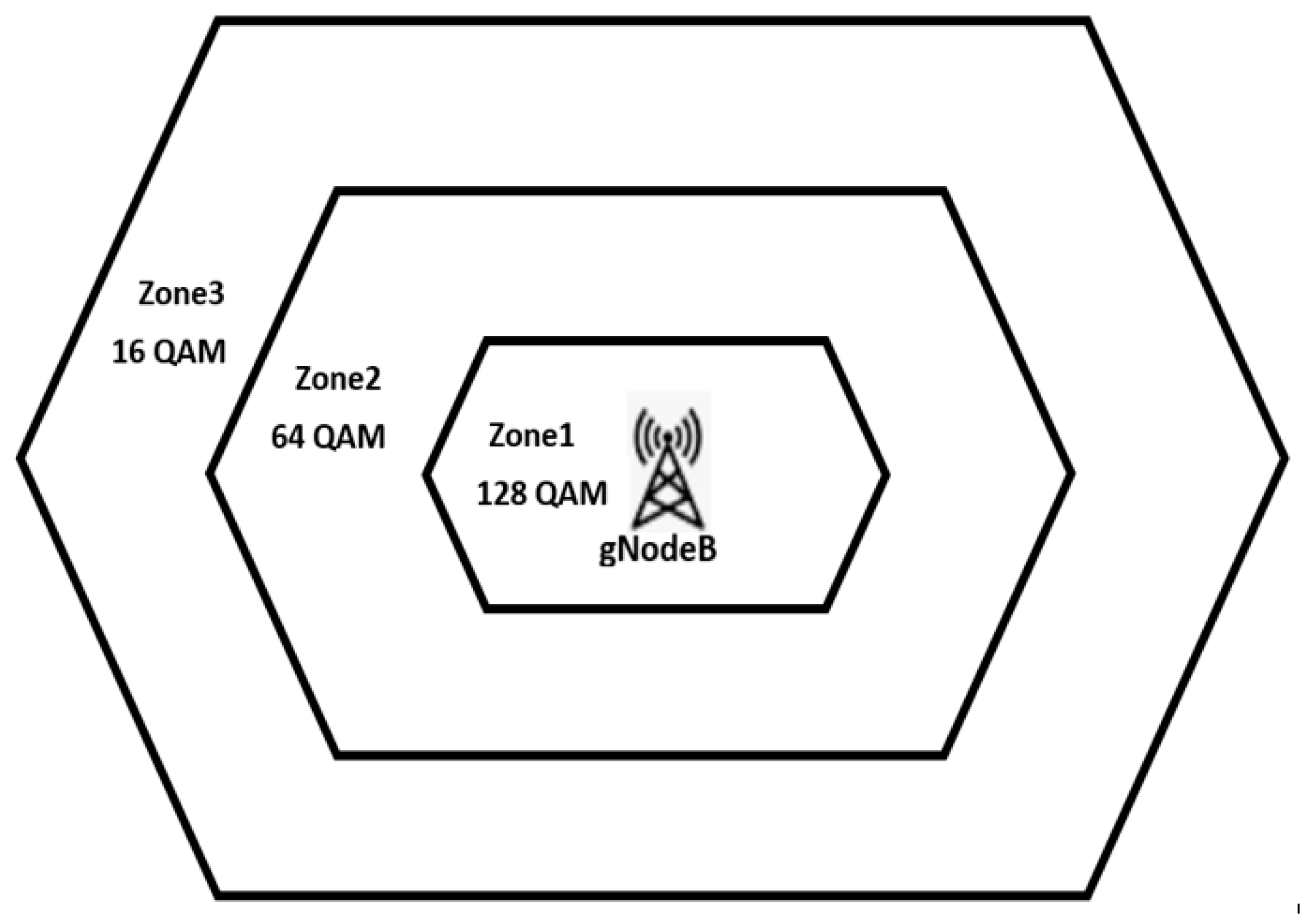
• We assume that a single 5G cell has the maximum capacity. The capacity is affected by the 5G modulation schemes and the maximum number of users in the cell.
• As per the modulation scheme in 5G, which is based on OFDMA (Orthogonal Frequency Division Multiple Access), the cell is divided into three virtual zones, as shown in Figure 4. According to 3GPP Release 15 [36,37], the physical layer of 5G downlinks uses different modulation schemes. Three modulation methods were assumed in this analysis, namely 128 Quadrature Amplitude Modulation (QAM) for zone 1 with 7 bits of transmitted information per symbol, 64 Quadrature Amplitude Modulation (QAM) for zone 2 with 6 bits of transmitted information per symbol, and 16 QAM for zone 3 with 4 bits.
• According to [37,38], we consider a cyclic prefix-based OFDM (CP-OFDM) waveform, which offers improved spectrum separation compared to LTE, to meet the diverse applications expected in 5G and reduce inter-cell interference (ICI) and inter-symbol interference (ISI).
• We assume a Poisson inter-arrival time $\lambda$ within the cell. The traffic load is determined based on the zone areas ($\alpha i\ast \lambda$, $i=1\dots$ zone $i$) and user density in the cell.
• The call admission control algorithm (CACA) relies on a minimum bit rate threshold that users must meet to be admitted to the system.
• The call admission control algorithm proposed in [12] was used in the proposed analysis.

5.2. Assumed Service Categories

In this analysis, three types of services are considered [39,40]:

(1)

Web browsing via a new radio (WBo5G): This service allows users to browse, find, and download web content from the internet at speeds exceeding one gigabyte. Because most internet activities involve web browsing, 60% of the available services are for this type of service.

(2)

Video Streaming-over-5G (STRo5G): This service provides real-time video streaming, video on demand (VoD), and virtual and augmented reality video experiences. To ensure minimal latency for multimedia services, 30% of all multimedia services are designated for this type of service.

(3)

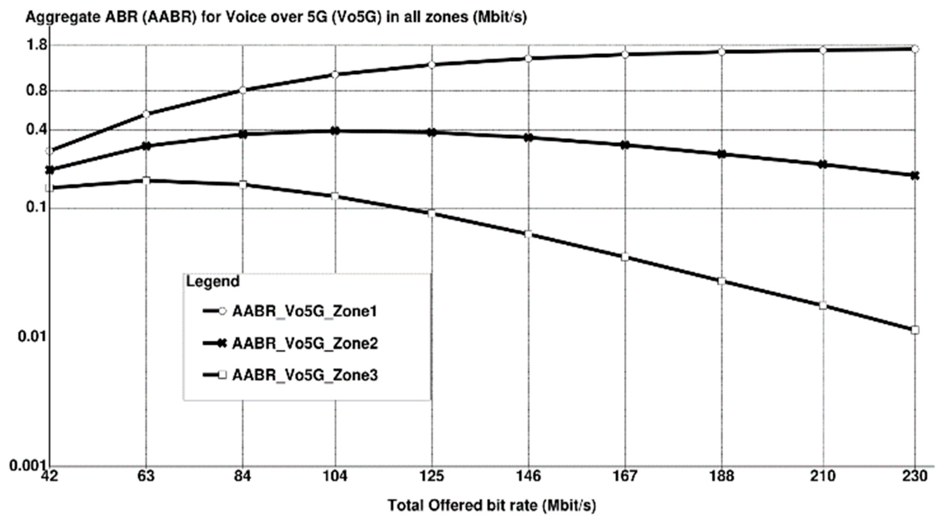
Voice-over-5G (Vo5G): Also known as voice over new radio, this provides high-definition (HD) voice communication for smartphones. It is infrequently used and is mainly reserved for emergency calls; thus, it constitutes the remaining 10% of all available services.

Regarding performance measures, the analysis yields the following performance parameters via the Continuous Time Markov Chain (CTMC) solver in the MOSEL-2 language [39,41]:

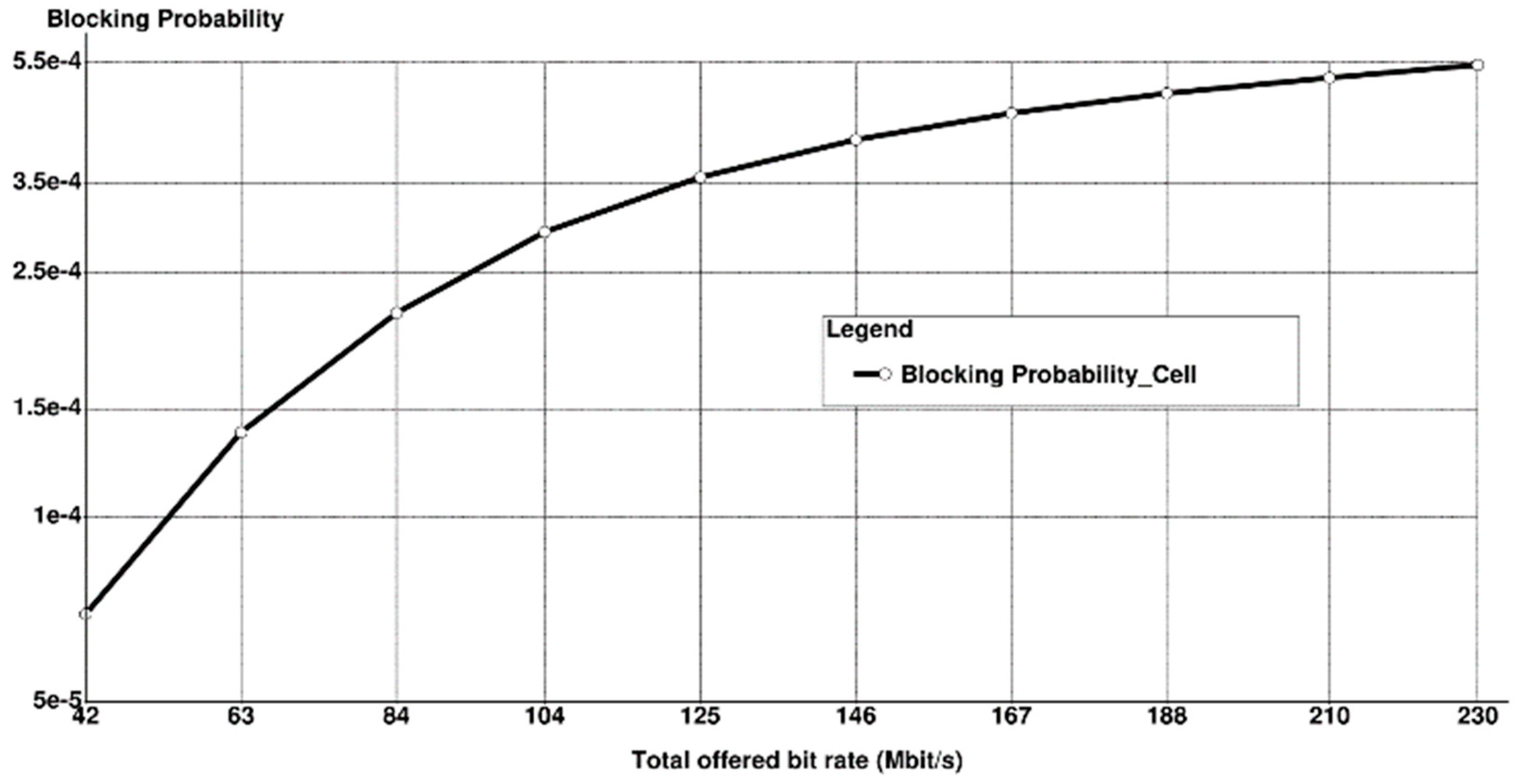
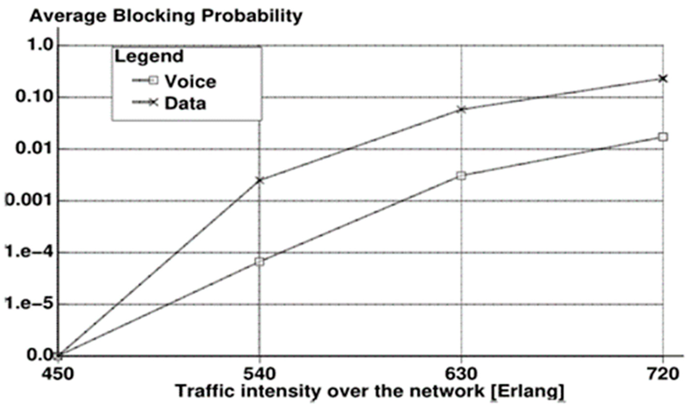
• Blocking Probability: The likelihood of call rejection if the call’s bit rate falls below the minimum threshold bit rate assumed in the cell.
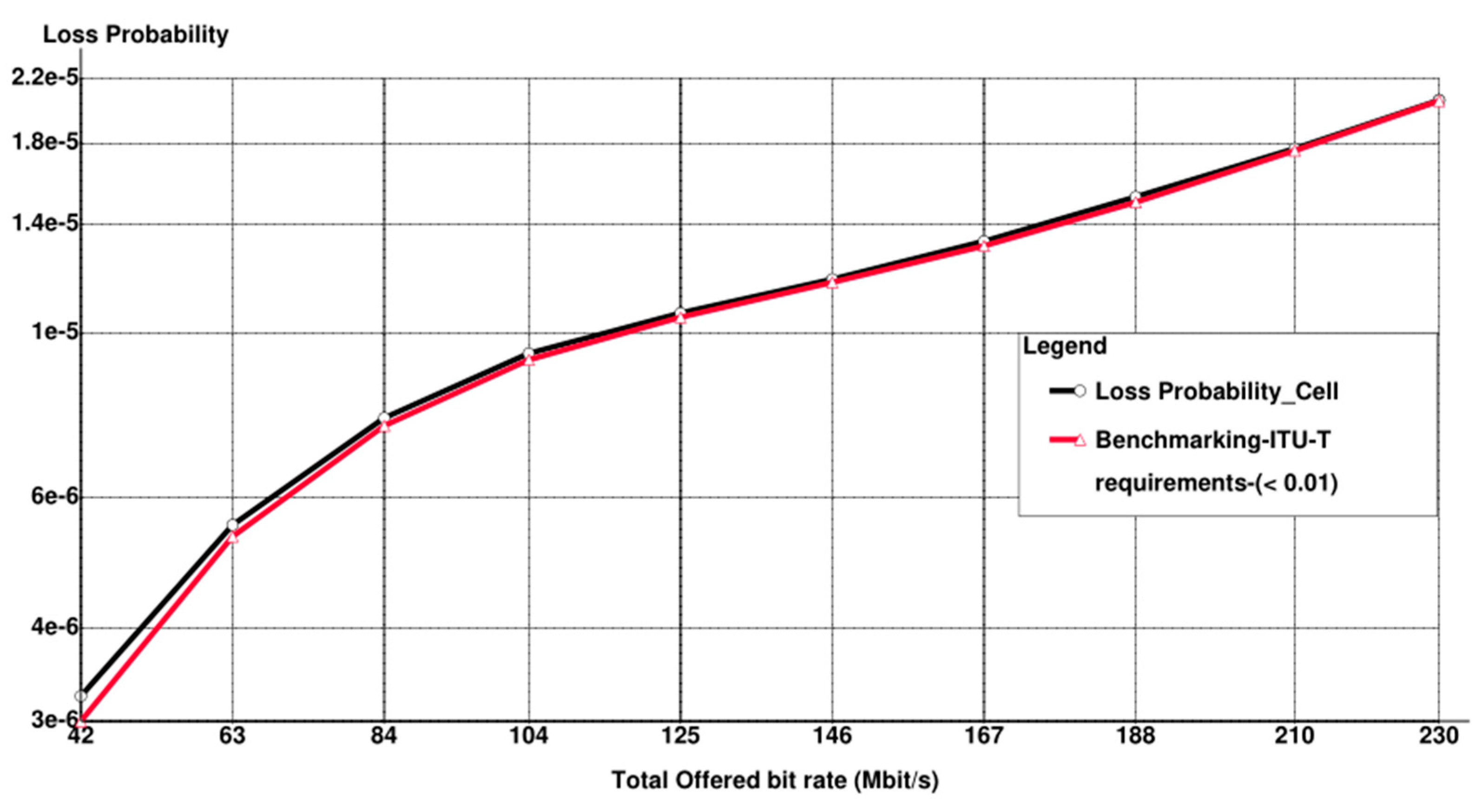
• Loss Probability: The likelihood of a call drop after admission when the user’s bit rate falls below the threshold value due to interference or channel quality degradation.
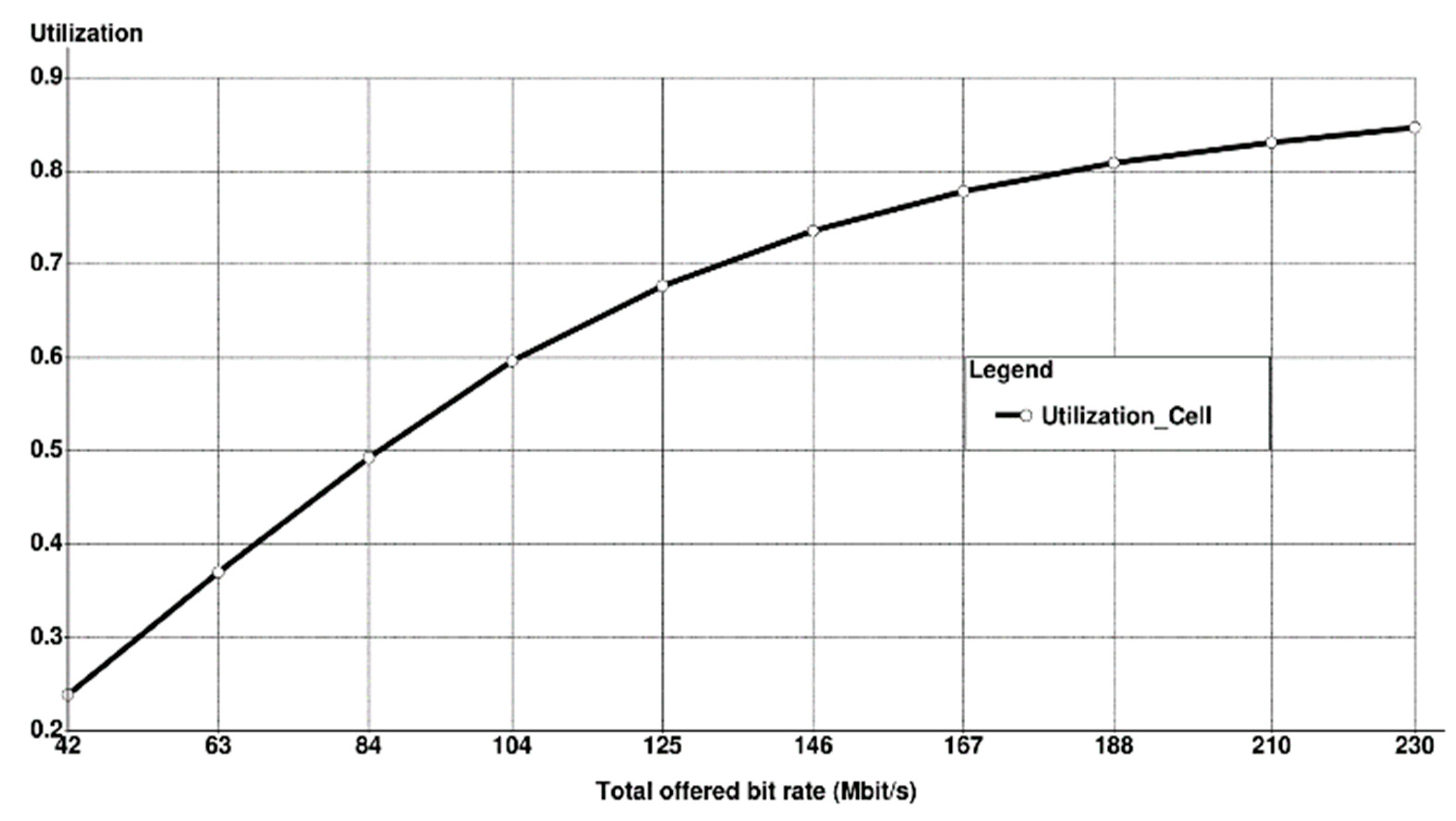
• Utilization: Average total bit rate relative to maximum cell capacity.
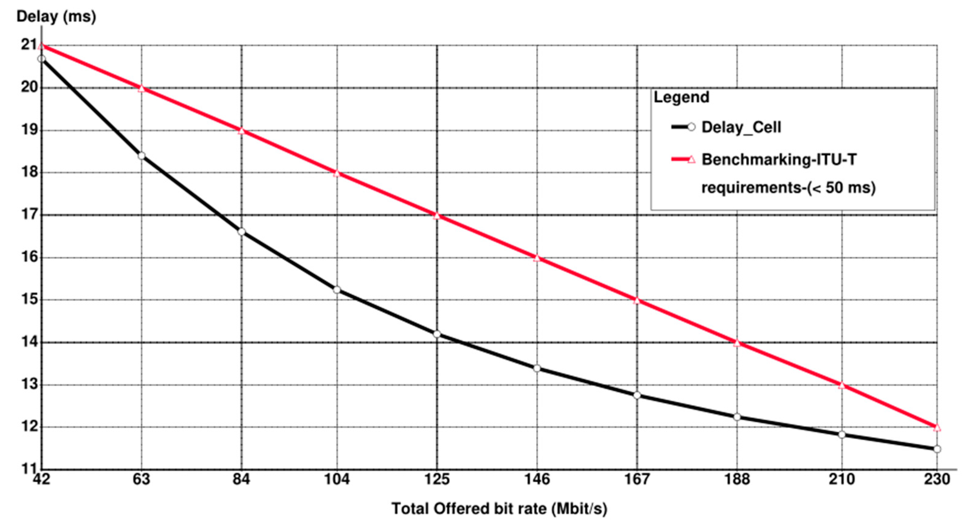
• Cell Delay: The time taken for a message to successfully reach its destination compared to the time the first bit is sent from the source.
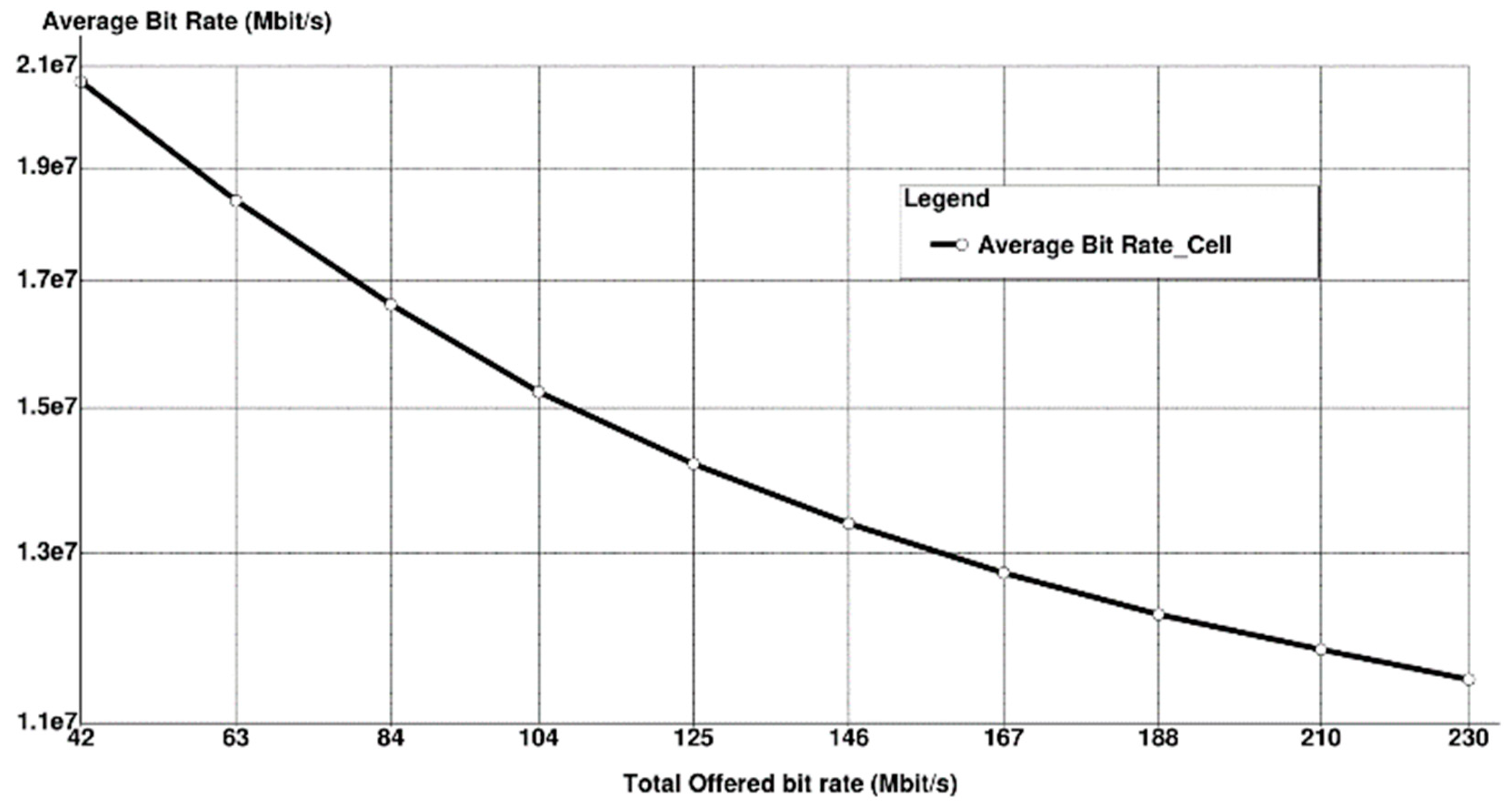
• Average Bitrate of the Cell: The mean total nitrate in the cell relative to the average session duration.
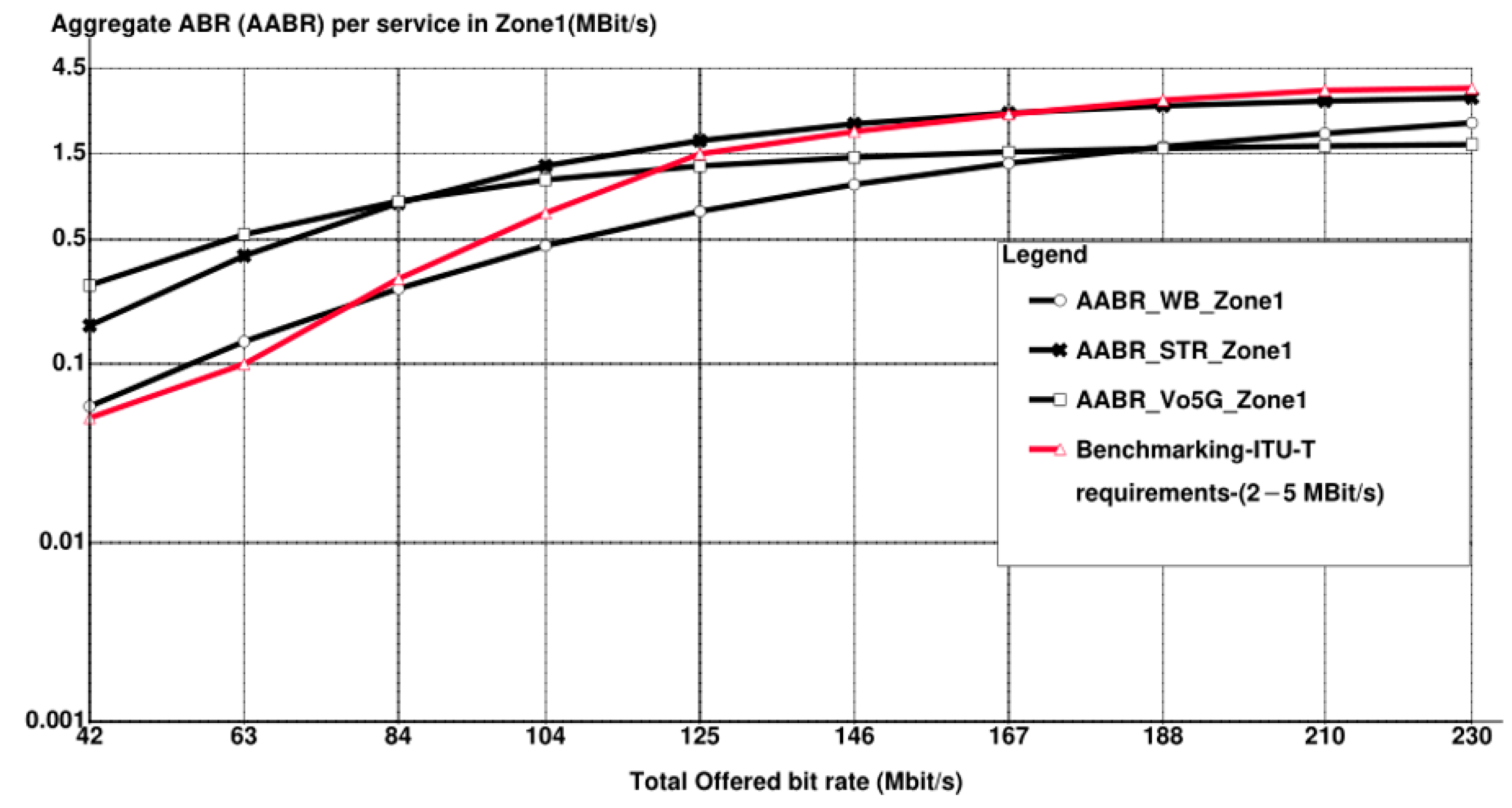
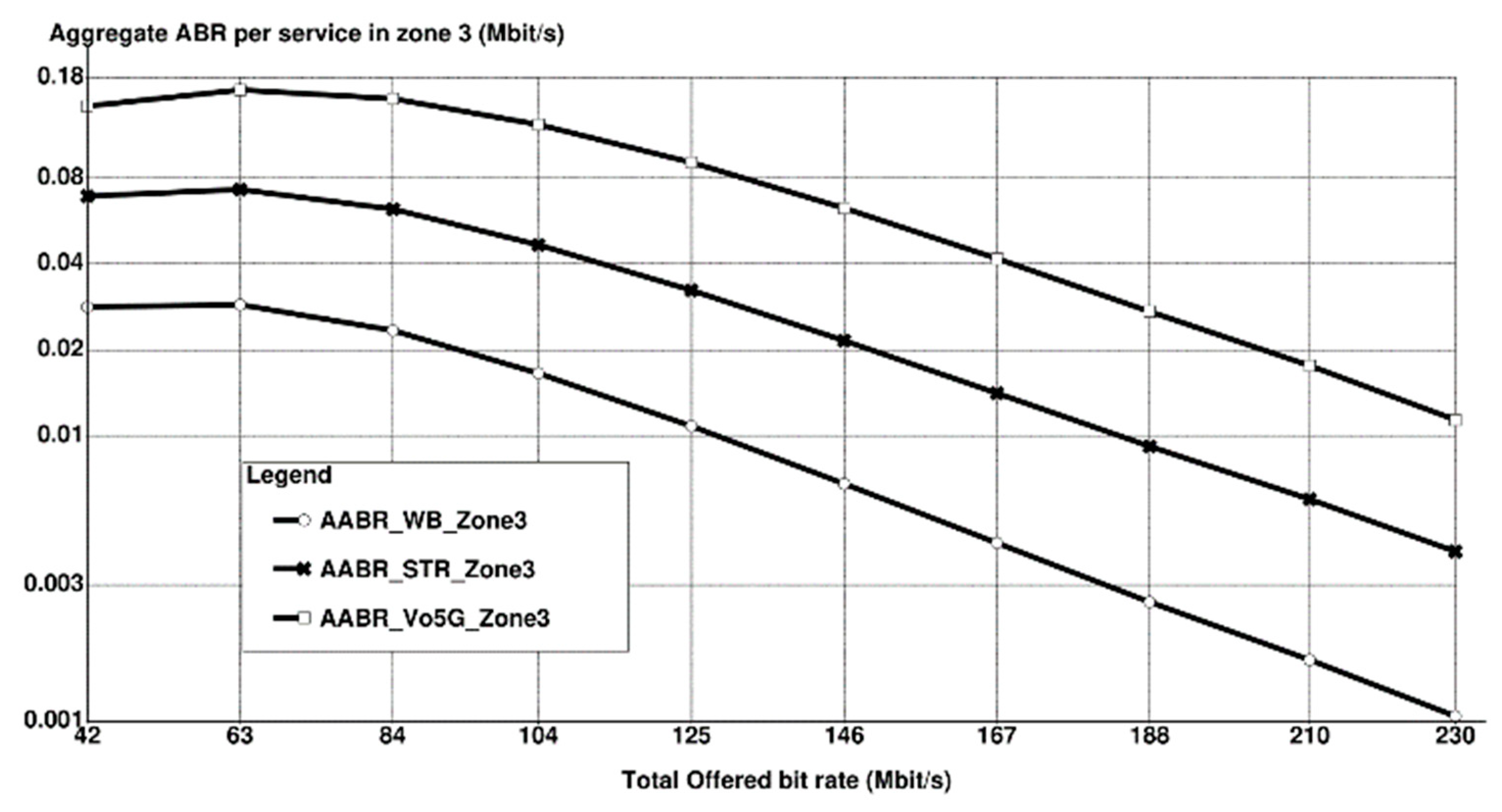
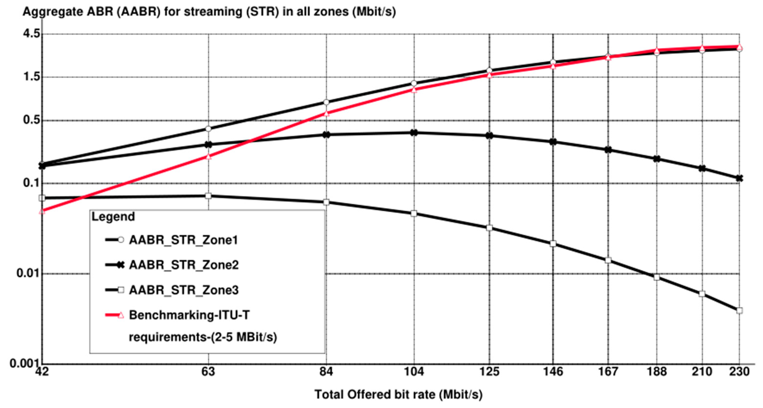
• Aggregate Bit Rate of the Cell: The average total bit rate across all services in the cell.
• Aggregate Bit Rate per Service: The aggregate bit rate is calculated as the average number of jobs in each service multiplied by the average bit rate required for that service’s area.
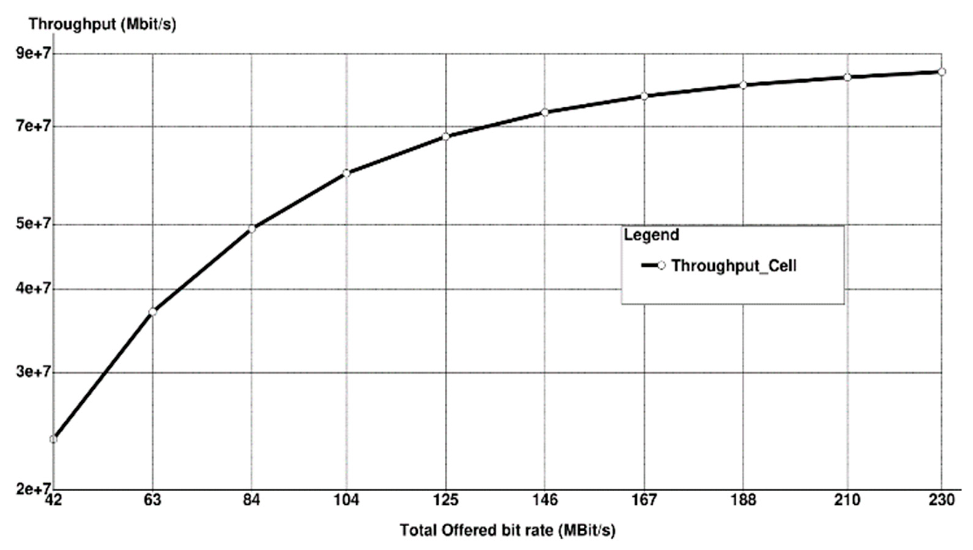
• Throughput: Calculated as the mean total bit rate in all zones for all services of the cell.

5.3. Mobility Model

When mobility is considered, either the transmitter or the receiver is in motion, and then we have a dynamic multipath situation in which there is a continuous change in the electrical length of every propagation path, and thus the relative phase shifts between them change as a function of spatial location. This phenomenon is called fast fading and should be taken into account in the propagation path loss because it causes large and rapid fluctuations in the signal. The rate of change in phase, due to motion, is apparent as a Doppler frequency shift in each propagation path, which is called the Doppler Effect, and accounts for fast fading. Therefore, the amount the frequency changes due to the Doppler Effect depends on the relative motion between the source and the receiver and on the speed of the mobile. Generally, frequency increases when moving toward the base station and decreases when moving away from the base station. The Doppler frequency has been considered to account for the effects of fast fading in the propagation model. Accordingly, Doppler or frequency shifts in the incident plane wave are incorporated, as shown in Figure 5 and referenced in [42].

Four kinds of users are represented in the simulation, where the amplitude is a Gaussian distribution with mean and standard deviation. The four kinds are as follows [43]:

(i) Stationary (mean speed $v_m=0 \mathrm{m}/\mathrm{s}$ and mean standard deviation (SD) $v_s=0 \mathrm{m}/\mathrm{s}$).

(ii) Slow speed (speed $v_m=4.0 \mathrm{m}/\mathrm{s}$, SD $v_s=0.5 \mathrm{m}/\mathrm{s}$).

(iii) Medium (speed $v_m=8.0 \mathrm{m}/\mathrm{s}$, SD $v_s=1.0 \mathrm{m}/\mathrm{s}$).

(iv) Fast (speed $v_m=12.0 \mathrm{m}/\mathrm{s}$, SD $v_s=1.0 \mathrm{m}/\mathrm{s}$).

Although the mobility parameters are determined randomly, as soon as the user arrives at the system, they will be assigned one of the above four mobility classes with equal probabilities. Whenever the user moves, his direction is turned by a random angle uniformly distributed between $-0.25\pi$ and $+0.25\pi$. Two types of services have been assumed (i.e., voice and data), and the arrival session for both voice and data is modeled as Poisson with the arrival rate, and the service time for the voice calls is exponentially distributed with a call duration of 180 s, whereas the data service time is modeled as a Pareto random variable to represent the self-similar behavior of WWW traffic. Data traffic is assumed to have a mean service time of 100 s. Pareto distribution parameters are given in

Table 2. Simulation parameters [44].

Parameter	Value
Average packet size-(Pareto distribution)	480 bytes
Average requested file size (25 × 480 bytes)-(Pareto distribution)	12 Kbytes
Average number of packet calls within a session-)-(Pareto distribution)	5
Average reading time between packet calls)-(Pareto distribution)	412 s
Average amount of packets within a packet call)-(Pareto distribution)	25
Average inter-arrival time between packets)-(Pareto distribution)	0.0625
Number of codes (N)	64
Frequency, f	20 GHz
Height of the mobile, hm	1.5 m
Base station height, hb	50 m
Service Factor, S(SF/SINR)	2–128
The cell radius r	0–20 Km
Spreading factor (SF)	32, 64, 128, 256 chips/symbol
Maximum transmission power (Psmax)	120 W
Thermal Noise, N0	−103 dBm
Signal-to-interference noise ratio (SNR)	2 dB
Interference factor, ε	0.30–0.70
Wavelength, λ	0.15 m
Number of zones	3
Ratio of web browsing	0.60
Ratio of streaming	0.30
Ratio of voice over 5G	0.10

.

For mobility analysis, the following performance metrics are assumed:

1. Dropping Probability (P_d) is the probability that the user is excluded from service after the handover.

2. Blocking Probability (P_b) is the probability that the new call arrival is rejected based on the CACA conditions.

3. Grade of Service (GoS = P_b + 10P_d) is the combination of the blocking and handover dropping probabilities in a weighted sum. The weighted sum of the new call-blocking probability and handoff-dropping probability is proposed in [43]. This scenario is under the assumption that the dropping probability affects the grade of service with a larger heightening factor than the blocking probability. This is true in real life. Moreover, this weighted average is very useful for most design purposes.

6. Simulation Results with Discussion

Numerical findings were created using MATLAB R2013b and MOSEL-2 simulations based on the parameters listed in Table 2. There are four groups of figures: the capacity and performance of 5G cells in a single-service scenario are the subjects of the first set of findings (Figure 6, Figure 7, Figure 8, Figure 9, Figure 10, Figure 11, Figure 12 and Figure 13). The second set of findings (Figure 14, Figure 15, Figure 16, Figure 17, Figure 18, Figure 19, Figure 20, Figure 21, Figure 22, Figure 23, Figure 24, Figure 25, Figure 26 and Figure 27) examines 3G cell performance and capacity in a multiservice case. The third group of results shows the network performance with multiservice cases and mobility (Figure 28, Figure 29, Figure 30, Figure 31, Figure 32, Figure 33, Figure 34, Figure 35 and Figure 36). The last groups of two figures (Figure 37 and Figure 38) are comparative results to compare the performance of the proposed algorithm in this research with a similar work in the literature [30].

Based on the developed equations for each environment, Figure 6 shows route loss under various propagation conditions.

Figure 6. Path loss in different propagation environments.

Figure 6. Path loss in different propagation environments.

It is evident that minimal loss values are attained in a free-space environment where there is an unobstructed line of sight between the transmitter and receiver. Additionally, losses are seen to be larger in rural regions than in open spaces, especially at distances greater than 5 km, as opposed to the free-space model, where there is a clear line of sight between the transmitter and receiver. Rural locations can also have airports and buildings, unlike free spaces, but they tend to have fewer people. Due to their high population density and packed building stock, dense metropolitan areas typically experience the highest path losses and hence suffer from signal radiation. Figure 7 shows the maximum distance separation from Node B for various service factor values. The data rate increased with a smaller service factor, whereas the coverage area decreased. As shown in Figure 7, the service only covers approximately 40 customers when S = 8, and these customers are located within a range of 6 km from Node B. In contrast, if S is 128, a round distance of 22 km can cover more than 500 users. The link between the cell capacity and cell radius is illustrated in Figure 8, along with the impact of various service characteristics.

As the cell radius is extended, it can be observed that at a larger value of S (S = 128), the capacity of the cell is maximized because many users can be accommodated. This graph demonstrates the positive correlation between the value of S and the cell radius measured from one side as well as the positive impact of this relationship on the cell’s overall capacity. The figures (Figure 8, Figure 9 and Figure 10) show similar behavior, but the goal is to show how the environment affects cell capacity. Higher S values increase system coverage and capacity. As shown in Figure 9, when S = 128 and the environment is a free space, the available service can cover 250 people even if the data rate for each user is reduced because all users share resources simultaneously

Figure 7. Maximum distance (coverage area vs. capacity).

Figure 7. Maximum distance (coverage area vs. capacity).

Figure 8. Cell capacities for different service factors (S).

Figure 8. Cell capacities for different service factors (S).

Figure 9. Cell capacities in different propagation environments (S = 128).

Figure 9. Cell capacities in different propagation environments (S = 128).

Figure 10 and Figure 11 exhibit similar behaviors. For example, in Figure 10, the S value decreases to 64; therefore, the number of active users goes down to 125, whereas when the S value in Figure 11 is 17, the number of active users decreases to 34. Apparently, the number of active users decreases as S decreases. Consequently, users benefit from a higher data rate. The final results of the first group are shown in Figure 12, which depicts the link between the distance from Node B and the capacity for three primary types of environments: dense urban, urban, and rural. For example, 150 users can be served within a 1.5 km distance in suburban areas, where people live with a lower population density than in metropolitan and dense urban areas. In contrast, the same number of users can be found approximately 0.9 km from Node B in urban regions and approximately 0.5 km in dense urban areas with high population density.

Figure 12 illustrates the phenomenon of cellular breathing, demonstrating that as the number of users in the cell increases, coverage decreases as a new user interferes with other users. This is an important signal that mobile operators should consider when developing future 5G networks.

Figure 10. Cell capacities in different propagation environments (S = 64).

Figure 10. Cell capacities in different propagation environments (S = 64).

Figure 11. Cell capacities in different propagation environments (S = 16).

Figure 11. Cell capacities in different propagation environments (S = 16).

Figure 12. Maximum distance in different propagation environments.

Figure 12. Maximum distance in different propagation environments.

Figure 13. Interference resulting in a maximum number of active users.

Figure 13. Interference resulting in a maximum number of active users.

Regarding the second group of results (Figure 13, Figure 14, Figure 15, Figure 16, Figure 17, Figure 18, Figure 19, Figure 20, Figure 21, Figure 22, Figure 23, Figure 24, Figure 25, Figure 26 and Figure 27), Figure 13 shows the maximum number of active users due to the interference in the multiservice case. It can be seen from this figure that the service factor parameter S has a major effect on the number of active users in the cell. The maximum number of successful admissions was achieved at service factor parameter values higher than small values. For example, the maximum number of active users reached 250 when S was 128, 60 when S was 32, and decreased to 16 when S was 8. Because the cell radius has a major effect on cell coverage, the capacity of the cell is shown in Figure 14 for different cell radii. The maximum number of active users (250 users) is obtained at a cell radius of 2 km and decreased to 100 users when the cell radius was increased to 9 km. In this case, Figure 14 presents an additional explanation of the cell breathing phenomenon, where the coverage of the cell is affected by the cell size and has a major effect on the maximum number of active users. Interference between users also has a major effect on cell capacity. Figure 15 shows that for the interference value (i.e., 0.30), around 200 users can be accepted. In contrast, for a 0.70 interference value, only 100 users were admitted to the system.

Figure 14. Uplink capacities of multiple channels.

Figure 14. Uplink capacities of multiple channels.

Figure 15. Uplink capacity for different interference factors, ε.

Figure 15. Uplink capacity for different interference factors, ε.

The aggregate average bit rate is presented in three figures (Figure 16, Figure 17 and Figure 18). The aggregate average bit rate is expected to be higher in zone 1 than in other zones because zone 1 has a higher achieved bit rate per user and improved modulation level in the cell. In Figure 16, the aggregate average bit rate is given in zone 1 for different service categories. Figure 16 shows that at a low rate (≤84 Mbit/s), a higher rate can be achieved for voice over 5G, and as soon as the load increases, the rate for streaming is increased and continues to achieve a higher average bit rate. At a lower rate, the number of users who requested a service was still small. However, users in zone 1 always enjoy higher bit rates than those in other zones regardless of the type of service being requested. To validate the results, the provided results in Figure 16 are compared against ITU-T requirements [44,45,46] for 5G networks. It can be noticed that benchmarking results are achieved on all types of services; however, the best results for streaming are achieved when the total offered bit rate increases (>125 Mbit/s). This is expected since real-time streaming needs a higher bit rate compared to voice and web browsing. We expect a lower average bit rate in zone 2 for all service categories, as illustrated in Figure 17, and it even decreases in zone 3, as illustrated in Figure 18. To confirm these results, the aggregate average bit rate is presented in Figure 19, Figure 20 and Figure 21 in all zones for each type of service. For example, in Figure 19, the streaming is shown in all zones, and it is shown more clearly that a maximum bit rate of around 3.5 Mbit/s can be achieved at a load of 230 Mbit/s in zone 1 compared to around 1.8 Mbit/s in zone 2 (Figure 20) and around 2.5 Mbit/s in zone 3 (Figure 21).

Figure 16. Aggregate average bit rate in zone 1.

Figure 16. Aggregate average bit rate in zone 1.

Figure 17. Aggregate average bit rate in zone 2.

Figure 17. Aggregate average bit rate in zone 2.

For more validation and confirmation of the status in Figure 16 regarding video streaming, the results are compared again in Figure 19 against ITU-T requirements. It can be noticed that the average bit rate required for video streaming is higher in zone 1 compared to other zones because the traffic density in zone 1 is higher. This is why better video streaming quality can be achieved at a higher offered bit rate (>104 Mbit/s). Starting from this rate, the video streaming levels start matching with the ITU-T requirements compared to the matching that happened earlier at lower bit rates for other services.

The overall cell performance is given in Figure 22, Figure 23, Figure 24, Figure 25, Figure 26 and Figure 27. Due to the use of the cyclic prefix method in 5G, inter-cell interference and inter-symbol interference will be improved. Subsequently, starting from Figure 22, the average bit rate in the entire cell is maximized to approximately 21 Mbit/s when the average bit rate is low (42 Mbit/s) because the overall number of users who request service at this load is small compared to 11 Mbit/s at a high bit rate of 230 Mbit/s. Therefore, few users will enjoy the maximum rate under all circumstances and for different service categories. When the load increases, the number of users increases, and the resources are shared with more users. This is why the performance of the cell degraded at higher loads (230 Mbit/s) (Figure 23) where a higher number of users were blocked.

Figure 18. Aggregate average bit rate in zone 3.

Figure 18. Aggregate average bit rate in zone 3.

Figure 19. Aggregate average bit rate for streaming across zones.

Figure 19. Aggregate average bit rate for streaming across zones.

Figure 20. Aggregate average bitrate for voice over 5G in all zones.

Figure 20. Aggregate average bitrate for voice over 5G in all zones.

The cell delay budget is shown in Figure 24. It can be noticed that optimal values for the cell delay budget are obtained as per the 3GPP and ITU-T standards [44,45,46]. The delay starts at approximately 20 ms at a bit rate of 42 Mbit/s and goes down to approximately 11 ms when the bit rate increases to 230 Mbit/s. For the sake of comparison and validation of the results, the cell delay budget in Figure 24 and the loss probability in Figure 25 are compared against the ITU-T requirements. It can clearly be seen in Figure 24 that the cell budget delay complies with the 3GPP and ITU-T requirements at different offered bit rates, and a good matching with the requirements is shown. Similar behavior can be noticed for the loss probability figure; however, regarding loss probability, complete matching with the requirement can be seen at a higher bit rate (>104 Mbit/s). This is a very good observation because when the offered bit rate increases, the probability of loss increases. To overcome this increase, the system needs an efficient call admission control algorithm. It appears that the call admission control algorithm works very well in terms of balancing the load over the cell. Typically, loss probability is more harmful to performance than blocking probability because, in loss probability, the call is blocked when it is in progress. However, a user is usually blocked or not admitted to the system when the admission conditions are not satisfied based on the applied call admission control algorithm. For example, in this case, the bit rate of the user is less than the threshold value of the minimum bit rate required for cell admission.

Fortunately, as shown in Figure 25, good results were obtained for the loss probability compared to the blocking probability values shown in Figure 23. For example, the maximum blocking rate shown in Figure 23 at a higher load of 230 Mbit/s is 0.00055 compared to 0.000022 for the loss probability at the same rate. The cell utilization is shown in Figure 26. In this figure, one can notice that the utilization of the cell is increased with the increased load, reaching around 85% at a high load of 230 Mibit/s. This result indicates that the cell performance is good, and the call admission control algorithm works well in terms of distrusting the load among users in the cell. In addition, this performance is confirmed by observing Figure 27, where a good throughput value is achieved.

Figure 21. Aggregate average bit rate for web browsing across zones.

Figure 21. Aggregate average bit rate for web browsing across zones.

Figure 22. Cell average bit rate.

Figure 22. Cell average bit rate.

Figure 23. Cell blocking probability.

Figure 23. Cell blocking probability.

Figure 24. Cell delay.

Figure 24. Cell delay.

Figure 25. Cell loss probability.

Figure 25. Cell loss probability.

Figure 26. Cell utilization.

Figure 26. Cell utilization.

Figure 27. Cell throughput.

Figure 27. Cell throughput.

In Figure 28, Figure 29, Figure 30, Figure 31, Figure 32, Figure 33, Figure 34, Figure 35 and Figure 36, the performance of the cell with voice and data services and the impact of mobility on the network performance are outlined. Furthermore, two scenarios are considered in the analysis. In the first scenario, the proportion of data services in the network is increased. As data require more bandwidth than voice, this should affect the performance of the network. In the second scenario, the proportion of mobiles moving at high speed is increased. This parameter should also affect performance. Looking at Figure 28, Figure 29 and Figure 30, one can notice that the handover dropping probability values (Figure 29) are better than the blocking probability values (Figure 28) at different traffic levels and under various mobility conditions with better performance for voice calls since data utilize more bandwidth than voice. In real life, dropping the call while being in progress is more annoying to the end user than blocking the new call. This effect is reflected in the GoS values given in Figure 30. Two additional scenarios are considered in this analysis:

(A) The impact of increasing the proportion of data services on the performance (Figure 31, Figure 32 and Figure 33).

In this scenario, the arrival density of data services is considered as 0.60 instead of 0.30. The average blocking probability is shown in Figure 31. It can be seen from this figure that the blocking probability values at different traffic intensities are higher than the handover-dropping probability values given in Figure 32. Due to this behavior, these results are reflected in the GoS values in Figure 33 because the GoS is a combination of the weighted sum of both the blocking and dropping probabilities. This status can be explained as follows. The proposed scenario is very realistic since the number of data services is nowadays expected to be more than the number of voice services as more people are using the internet. Of course, doubling the proportion of data services will have a major impact on performance. Regardless of the performance degradation, the CACA was able to stabilize the status by keeping the dropping probability values at lower rates.

(B) The impact of more mobiles are moving with high speed (Figure 34, Figure 35 and Figure 36). In this scenario, the probability of having 40% high-speed mobiles in the network rather than 10% is considered. In this regard, in Figure 34 for the blocking probability, Figure 35 for the handover dropping probability, and Figure 36 for the GoS, it can be noticed that due to this increase, the overall performance of the network degrades. For example, one can notice from Figure 33 that at low-speed mobile, the blocking probability at traffic intensity of 450 Erlang is less than 0.10 for data service and around 0.001 for voice service; on the other hand, considering high-speed mobiles and at the same traffic intensity of 450 Erlang, clear degradation of the performance occurs where the blocking in Figure 34 is more than 0.10 for data service and around 0.01 for voice service. This status can be explained as follows. In real life, the signal strength fluctuates while being on the move. In all circumstances, thanks to the CACA, it works well in balancing the load all over the network and keeping the blocking and dropping probability at lower levels.

In the final set of results [37,38], the proposed algorithm is evaluated against similar findings from [30]. According to [30], the outcomes are presented for the average number of dropped packets (Figure 37) and the average utility performance (Figure 38) relative to the data arrival rate (Mbit/s). It is evident from Figure 37 that up to an arrival rate of 2.7 Mbit/s, there is nearly a total correspondence between our algorithm and the one proposed in [30]. However, when the rate exceeds 2.7 Mbit/s, our algorithm demonstrates superiority over the suggested method by achieving a better performance in terms of the number of packets dropped. Conversely, from Figure 38, it is clear that our algorithm exceeds the performance of the proposed algorithm across all traffic levels. This is predictable since the authors in [30] indicated that an increase in locally processed computational tasks results in an increase in CPU energy consumption, which leads to a decline in performance.

Figure 28. Average blocking probability.

Figure 28. Average blocking probability.

Figure 29. Average handover dropping probability.

Figure 29. Average handover dropping probability.

Figure 30. Grade of service (GoS).

Figure 30. Grade of service (GoS).

Figure 31. Average blocking probability with a 60% increase in the proportion of data services..

Figure 31. Average blocking probability with a 60% increase in the proportion of data services..

Figure 32. Average handover dropping probability with a 60% increase in the proportion of data services..

Figure 32. Average handover dropping probability with a 60% increase in the proportion of data services..

Figure 33. Grade of service (GoS) with a 60% increase in the proportion of data services..

Figure 33. Grade of service (GoS) with a 60% increase in the proportion of data services..

Figure 34. Average blocking probability with 40% high-speed mobile users.

Figure 34. Average blocking probability with 40% high-speed mobile users.

Figure 35. Average handover dropping probability Average blocking probability with 40% high-speed mobile users. .

Figure 35. Average handover dropping probability Average blocking probability with 40% high-speed mobile users. .

Figure 36. Grade of service (GoS) Average blocking probability with 40% high-speed mobile users..

Figure 36. Grade of service (GoS) Average blocking probability with 40% high-speed mobile users..

Figure 37. Comparative results—average number of packets dropped.

Figure 37. Comparative results—average number of packets dropped.

Figure 38. Comparative results—average utility performance.

Figure 38. Comparative results—average utility performance.

7. Conclusions and Future Considerations

Wireless network designers and operators in 5G and beyond confront difficult expectations such as greater capacity, higher data rates, lower latency, and improved connectivity for many users. Due to propagation phenomena induced by reflection and diffraction in wireless networks, a sent signal is received by the receiver with numerous copies at various amplitudes, delays, and arrival angles. Therefore, the signal strengths of such systems must be considered. Because the free space model does not consider external impediments, it is important to evaluate the performance of such systems in realistic contexts. The system performance was analyzed and discussed after establishing capacity limitations in different propagation scenarios while accounting for cell interference, limited uplink power, and mobility. The numerical findings and analysis reveal that the type of environment and service factor parameters have the greatest influence on system capacity and coverage. Moreover, it shows that the cell radii also have a major effect on the cell capacity and coverage justified in the numerical results by the cell breathing phenomena. In this regard, it is shown that there is a positive correlation between the service factor value and the cell radius; therefore, the optimization of this relationship will have a positive impact on the cell capacity. The investigations, analyses, and findings presented provide vital indicators for mobile designers and operators to consider in future 5G network development. Moreover, some results are evaluated against ITU-T standards, while others are compared with related studies from the literature for the purpose of validating the findings. This study can be extended to a multi-cell situation in which a seamless 5G handover between the original and neighboring cells is examined.

The main limitations of this research are as follows.

○

Although the proposed CACA works on a network level of this system, only one cell was considered in the analysis and discussion. This work should be extended to a network-level scenario considering 5G seamless handover between the original and neighboring cells.

○

Due to the scarcity of resources in the literature with similar scenarios in this research and not deviating from the main objective of this research, it was not possible to conduct a comparison with other works in the literature. However, for the sake of validation, a benchmarking of ITU-T QoS requirements for 5G is added to some results.

○

In future research directions, the above limitations will be considered.

References

- Chen, S.; Kaushik, A.; Masouros, C. Pre-scaling and codebook design for joint radar and communication based on index modulation. In Proceedings of the IEEE Global Communications Conference (GLOBECOM), Rio de Janeiro, Brazil, 4–8 December 2022; pp. 1–5. [Google Scholar]
- Huang, T.; Shlezinger, N.; Xu, X.; Liu, Y.; Eldar, Y.C. MAJoRCom: A dual-function radar communication system using index modulation. IEEE Trans. Signal Process 2020, 68, 3423–3438. [Google Scholar] [CrossRef]
- Ma, H.; Fang, Y.; Chen, P.; Mumtaz, S.; Li, Y.A. Novel Differential Chaos Shift Keying Scheme With Multidimensional Index Modulation. IEEE Trans. Wirel. Commun. 2023, 22, 237–256. [Google Scholar] [CrossRef]
- Lee, H.; Shin, S. A novel index modulation scheme with impedance matching. Indones. J. Electr. Eng. Comput. Sci. 2019, 14, 1203–1209. [Google Scholar] [CrossRef]
- Cheng, X.; Zhang, M.; Wen, M.; Yang, L. Index Modulation for 5G: Striving to Do More with Less. IEEE Wirel. Commun. 2018, 25, 126–132. [Google Scholar] [CrossRef]
- Mgobhozi, B.; Nleya, B. Efficient Index Modulation Techniques for 5G and Beyond. In Proceedings of the 2023 International Conference on Electrical, Computer and Energy Technologies (ICECET), Cape Town, South Africa, 16–17 November 2023; pp. 1–6. [Google Scholar] [CrossRef]
- Doğan Tusha, S.; Tusha, A.; Basar, E.; Arslan, H. Multidimensional Index Modulation for 5G and Beyond Wireless Networks. Proc. IEEE 2021, 109, 170–199. [Google Scholar] [CrossRef]
- Deng, T.; Ding, J.; Liang, P. Investigating and Applying Orthogonal Frequency Division Multiplexing with Index Modulation. In Proceedings of the 2024 4th Asia-Pacific Conference on Communications Technology and Computer Science (ACCTCS), Shenyang, China, 24–26 February 2024; pp. 791–794. [Google Scholar] [CrossRef]
- Bouhlel, A.; Sakly, A.; Ikki, S. Performance analysis of DWT based OFDM with index modulation under channel estimation error. In Proceedings of the 2017 International Conference on Engineering & MIS (ICEMIS), Monastir, Tunisia, 11 December 2017; pp. 1–5. [Google Scholar] [CrossRef]
- Öztürk, E.; Basar, E.; Çırpan, H.A. Generalized Frequency Division Multiplexing With Flexible Index Modulation Numerology. IEEE Signal Process. Lett. 2018, 25, 1480–1484. [Google Scholar] [CrossRef]
- Kadir, M.I. Generalized Space–Time–Frequency Index Modulation. IEEE Commun. Lett. 2019, 23, 250–253. [Google Scholar] [CrossRef]
- Zreikat, A.I. Load balancing call admission control algorithm (CACA) based on soft-handover in 5G Networks. In Proceedings of the 2022 IEEE 12th Annual Computing and Communication Workshop and Conference (CCWC2022), Las Vegas, NV, USA, 26–29 January 2022; pp. 863–869. [Google Scholar]
- Zreikat, A.I.; Al-abed, S. Performance Modeling and Analysis of LTE/Wi-Fi Coexistence. Electronics 2022, 11, 1035. [Google Scholar] [CrossRef]
- Chen, J.; Lin, W.; Yan, P.; Xu, J.; Hou, D.; Hong, W. Design of mm-Wave transmitter and receiver for 5G. In Proceedings of the 2017 10th Global Symposium on Millimeter-Waves, Hong Kong, China, 24–26 May 2017; pp. 92–93. [Google Scholar] [CrossRef]
- Banaseka, F.K.; Dotse, S. New deployments and Research challenges for 5G wireless systems and networks. Int. J. Curr. Res. 2017, 9, 46626–46631. [Google Scholar]
- Hata, M. Empirical formula for propagation loss in land mobile radio services. IEEE Trans. Veh. Technol. 1980, 29, 317–325. [Google Scholar] [CrossRef]
- Nkordeh, N.S.; Atayero, A.A.A.; Idachaba, F.E.; Oni, O.O. LTE Network Planning using the Hata-Okumura and the COST-231 Hata Path loss Models. In Proceedings of the World Congress on Engineering 2014 (Vol I, WCE 2014), London, UK, 2–4 July 2014. [Google Scholar]
- Zreikat, A.I. Capacity Bounds Analysis of 5G networks in different propagation environments. In Proceedings of the 2023 IEEE 13th Annual Computing and Communication Workshop and Conference (CCWC), Las Vegas, NV, USA, 8–11 March 2023; pp. 988–993. [Google Scholar] [CrossRef]
- Preben, M.; Wei, N.; Istvan, Z.K.; Frank, F.; Akhilesh, P.; Klaus, I.P.; Troels, K.; Klaus, H.; Markku, K. LTE Capacity Compared to the Shannon Bound. In Proceedings of the 2007 IEEE 65th Vehicular Technology Conference (VTC2007-Spring), Dublin, Ireland, 22–25 April 2007; pp. 1234–1238. [Google Scholar] [CrossRef]
- Dutta, S.; Khalili, A.; Erkip, E.; Rangan, S. Capacity Bounds for Communication Systems with Quantization and Spectral Constraints. In Proceedings of the 2020 IEEE International Symposium on Information Theory (ISIT), Los Angeles, CA, USA, 21–26 June 2020; pp. 2038–2043. [Google Scholar] [CrossRef]
- Zhang, X.; Wang, J.; Poor, H.V. Statistical Delay-Bounded QoS Provisioning Over 5G Multimedia Mobile Wireless Networks in the Finite Blocklength Regime. In Proceedings of the ICC 2019—2019 IEEE International Conference on Communications (ICC), Shanghai, China, 20–24 May 2019; pp. 1–6. [Google Scholar] [CrossRef]
- Xiao, L.; Xiao, P.; Liu, Z.; Yu, W.; Haas, H.; Hanzo, L. A Compressive Sensing Assisted Massive SM-VBLAST System: Error Probability and Capacity Analysis. IEEE Trans. Wirel. Commun. 2020, 19, 1990–2005. [Google Scholar] [CrossRef]
- Zhao, W.; Wang, G.; Ai, B.; Li, J.; Tellambura, C. Backscatter Aided Wireless Communications on High-Speed Rails: Capacity Analysis and Transceiver Design. IEEE J. Sel. Areas Commun. 2020, 38, 2864–2874. [Google Scholar] [CrossRef]
- Tlebaldiyeva, L.; Maham, B.; Tsiftsis, T.A. Capacity Analysis of Device-to-Device mmWave Networks Under Transceiver Distortion Noise and Imperfect CSI. IEEE Trans. Veh. Technol. 2020, 69, 5707–5712. [Google Scholar] [CrossRef]
- Papazafeiropoulos, A.K.; Sharma, S.K.; Chatzinotas, S.; Ottersten, B. Ergodic Capacity Analysis of AF DH MIMO Relay Systems With Residual Transceiver Hardware Impairments: Conventional and Large System Limits. IEEE Trans. Veh. Technol. 2017, 66, 7010–7025. [Google Scholar] [CrossRef]
- Cao, F.; Han, Y.; Liu, Q.; Wen, C.-K.; . Jin, S. Capacity Analysis and Scheduling for Distributed LIS-aided Large-Scale Antenna Systems. In Proceedings of the 2019 IEEE/CIC International Conference on Communications in China (ICCC), Changchun, China, 11–13 August 2019; pp. 659–664. [Google Scholar] [CrossRef]
- Nossire, Z.; Gupta, N.; Almazaydeh, L.; Xiong, X. New Empirical Path Loss Model for 28 GHz and 38 GHz Millimeter Wave in Indoor Urban under Various Conditions. Appl. Sci. 2018, 8, 2122. [Google Scholar] [CrossRef]
- Parsons, J.D. The Mobile Radio Propagation Channel, 2nd ed.; John Wiley & Sons: New York, NY, USA, 2000; pp. 16–17, 75–77, 116–118. [Google Scholar]
- Wang, C.; Deng, D.; Xu, L.; Wang, W.; Gao, F. Joint Interference Alignment and Power Control for Dense Networks via Deep Reinforcement Learning. IEEE Wirel. Commun. Lett. 2021, 10, 966–970. [Google Scholar] [CrossRef]
- Chen, X.; Wu, C.; Liu, Z.; Zhang, N.; Ji, Y. Computation Offloading in Beyond 5G Networks: A Distributed Learning Framework and Applications. IEEE Wirel. Commun. 2021, 28, 56–62. [Google Scholar] [CrossRef]
- Mogensen, P.E.; Wigard, J. COST Action 231: Digital Mobile Radio—Towards Future Generation Systems; Final Report, EUR 18957, Chapter 4; European Commission: Brussels, Belgium, 1999. [Google Scholar]
- Zreikat, A.I. Radio Resource Management and Modeling for Wireless Mobile Networks: Enhancement of Call Admission Control Algorithms (CACAs) and Capacity Bounds in UMTS/GSM Networks; LAMBERT Academic Publishing: Saarbrücken, Germany, 2011; 216p, ISBN 3846534994/978-3846534991. [Google Scholar]
- Benni, N.S.; Manvi, S.S. Clustering Algorithm To Mitigate Intra And Inter-Cell Interference In 5G Backhaul Wireless Mesh Networks. In Proceedings of the 2022 IEEE 19th India Council International Conference (INDICON), Kochi, India, 24–26 November 2022; pp. 1–8. [Google Scholar] [CrossRef]
- Holma, H.; Toskala, A. WCDMA for UMTS: Radio Access for Third Generation Mobile Communications, 2nd ed.; John Wiley & Sons: New York, NY, USA, 2002; pp. 167–248. [Google Scholar]
- Holma, H.; Laakso, J. Uplink admission control and soft capacity with MUD in CDMA. In Proceedings of the Gateway to 21st Century Communications Village. VTC 1999-Fall. IEEE VTS 50th Vehicular Technology Conference (Cat. No.99CH36324), Amsterdam, The Netherlands, 19–22 September 1999; pp. 431–435. [Google Scholar] [CrossRef]
- ITU: 5G networks and 3GPP Release 15. Available online: https://www.itu.int/en/ITU-D/Regional-Presence/AsiaPacific/SiteAssets/Pages/ITU-ASP-CoE-Training-on-/session7_5G%20networks%20and%203GPP%20release%2015.pdf (accessed on 18 July 2024).
- 3GPP-TS 138.214. Release 16.2.0 5G NR. Available online: https://www.etsi.org/deliver/etsi_ts/138200_138299/138214/16.02.00_60/ts_138214v160200p.pdf (accessed on 14 July 2024).
- Tong, W.; Ma, J.; Zhu Huawei, P. Enabling technologies for 5G air interface with emphasis on spectral efficiency in the presence of very large number of links. In Proceedings of the 2015 21st Asia-Pacific Conference on Communications (APCC), Kyoto, Japan, 14–16 October 2015; pp. 184–187. [Google Scholar] [CrossRef]
- Zreikat, A.I.; Mathew, S. Performance Evaluation and analysis of Urban-Suburban 5G Cellular Networks. Computers 2024, 13, 108. [Google Scholar] [CrossRef]
- Zreikat, A.I.; Mercan, S. Performance Study of 5G Downlink Cell. In Internet of Things, Smart Spaces, and Next Generation Networks and Systems, Proceedings of the 6th International Conference, NEW2AN 2006, St. Petersburg, Russia, 29 May–2 June 2006; Lecture Notes in Computer Science; Galinina, O., Andreev, S., Balandin, S., Koucheryavy, Y., Eds.; Springer: Cham, Switzerland, 2019; p. 11660. [Google Scholar] [CrossRef]
- MOSEL Home Page. Available online: https://www4.cs.fau.de/Projects/MOSEL/ (accessed on 15 July 2024).
- Badia, L.; Zorzi, M.; Gazzini, A. On the impact of user mobility on call admission control in WCDMA systems. In Proceedings of the IEEE 56th Vehicular Technology Conference, Vancouver, BC, Canada, 24–28 September 2002; Volume 1, pp. 121–126. [Google Scholar] [CrossRef]
- Candan, I.; Salamah, M. Dynamic Time-Threshold Based Scheme for Voice Calls in Cellular Networks. In Next Generation Teletraffic and Wired/Wireless Advanced Networking, Proceedings of the 6th International Conference, NEW2AN 2006, St. Petersburg, Russia, 29 May–2 June 2006; Lecture Notes in Computer Science; Koucheryavy, Y., Harju, J., Iversen, V.B., Eds.; Springer: Berlin/Heidelberg, Germany, 2006; Volume 4003. [Google Scholar] [CrossRef]
- TSG-RAN Working Group 1 Meeting #6. Available online: https://www.3gpp.org/ftp/tsg_ran/wg1_rl1/TSGR1_06/Docs/Pdfs/r1-99818.pdf (accessed on 8 January 2025).
- Radio Access Network (RAN) Delay Budget Reporting in the Multimedia Telephony Service for Internet Protocol (IP) Multimedia Subsystem (IMS) (MTSI). Available online: https://www.etsi.org/deliver/etsi_tr/126900_126999/126910/16.00.00_60/tr_126910v160000p.pdf (accessed on 25 July 2024).
- Tarafder, P.; Chun, C.; Ullah, A.; Kim, Y.; Choi, W. Channel Estimation in 5G-and-Beyond Wireless Communication: A Comprehensive Survey. Electronics 2025, 14, 750. [Google Scholar] [CrossRef]