


The Robust Control of a Nonsmooth or Switched Control-Affine Uncertain Nonlinear System Using an Auxiliary Robust Integral of the Sign of the Error (ARISE) Controller †

Abstract
1. Introduction
2. Materials and Methods
2.1. Dynamics
2.2. Controller Design
2.3. Stability Analysis
2.4. Simulation
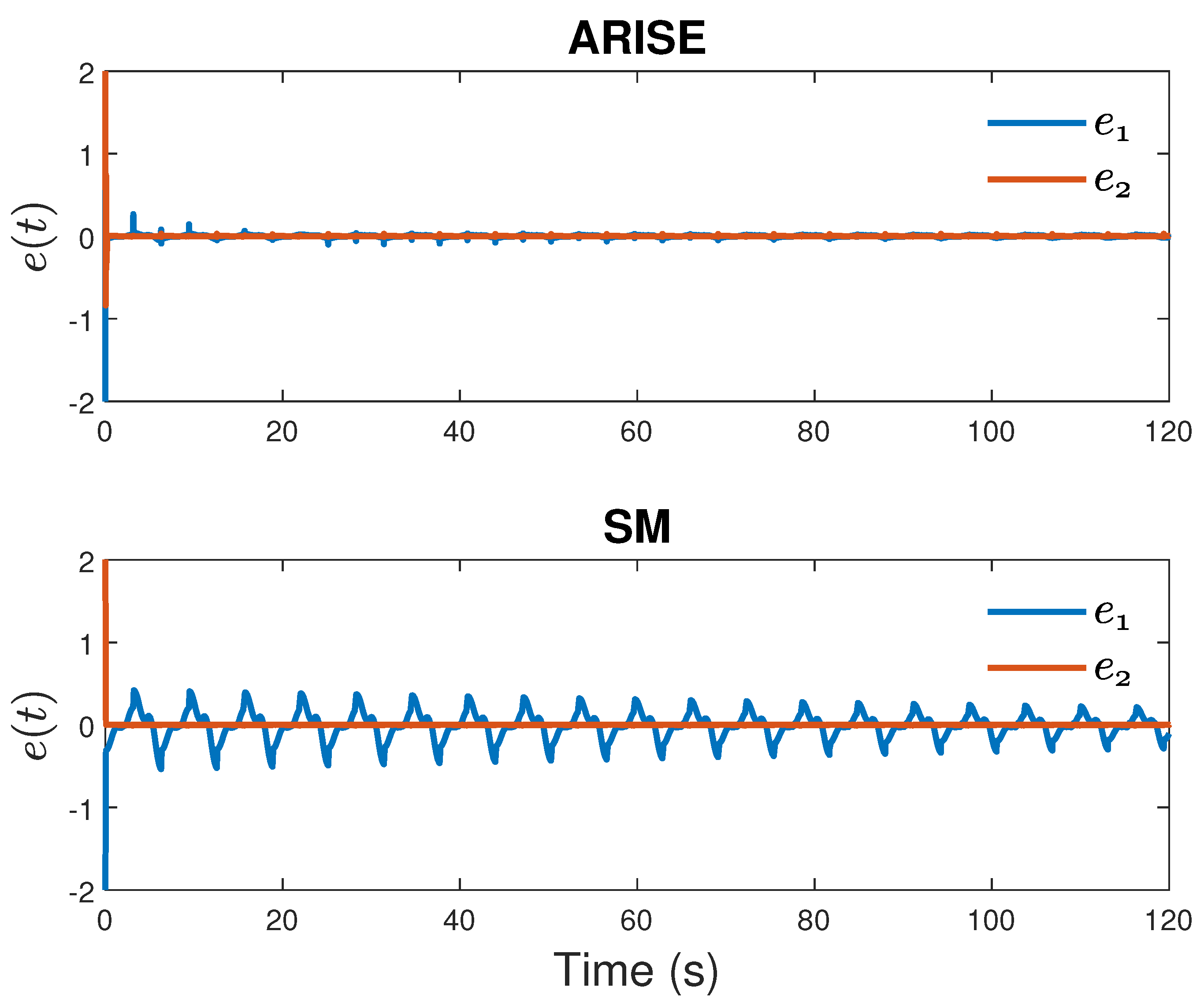
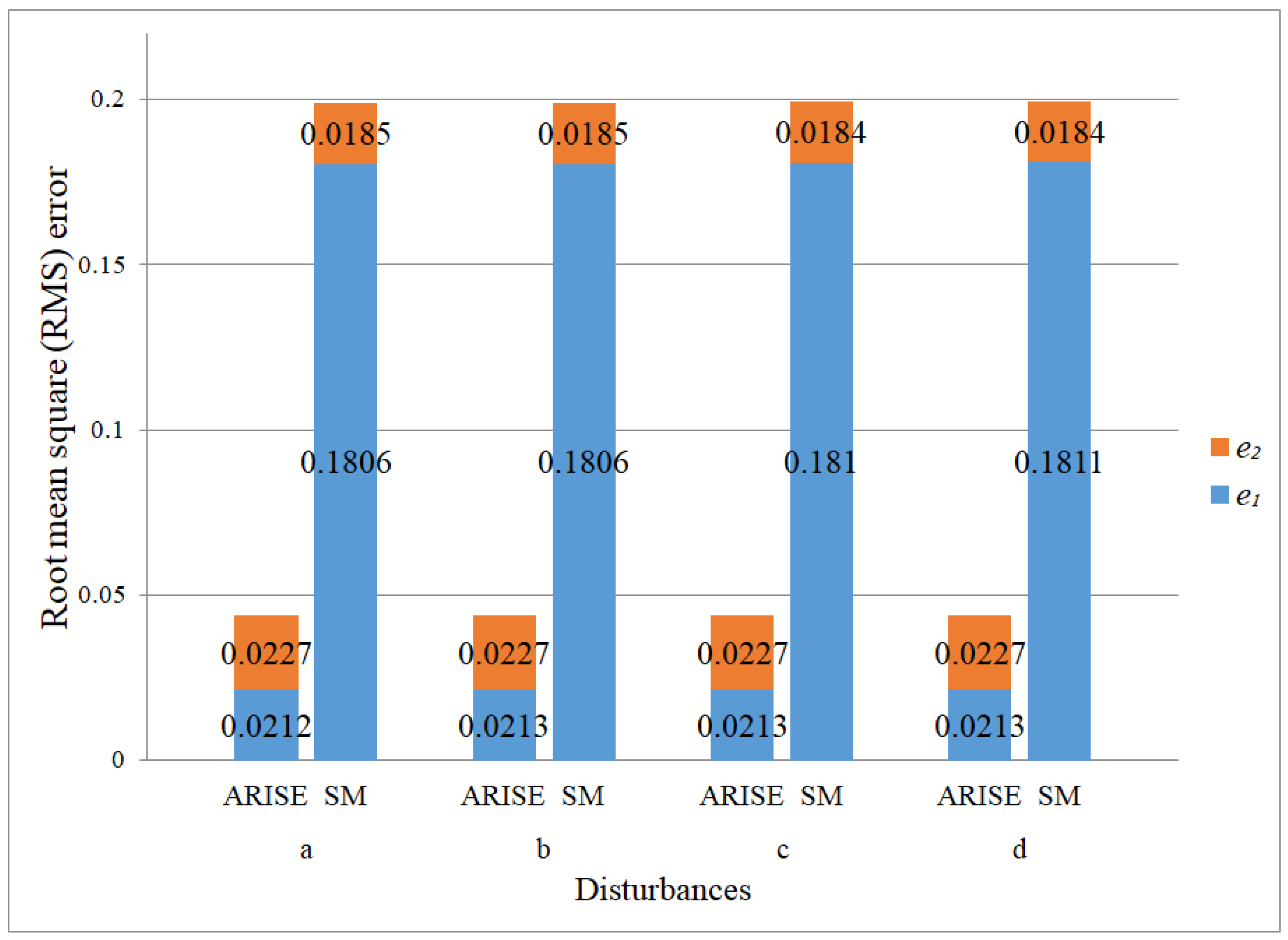
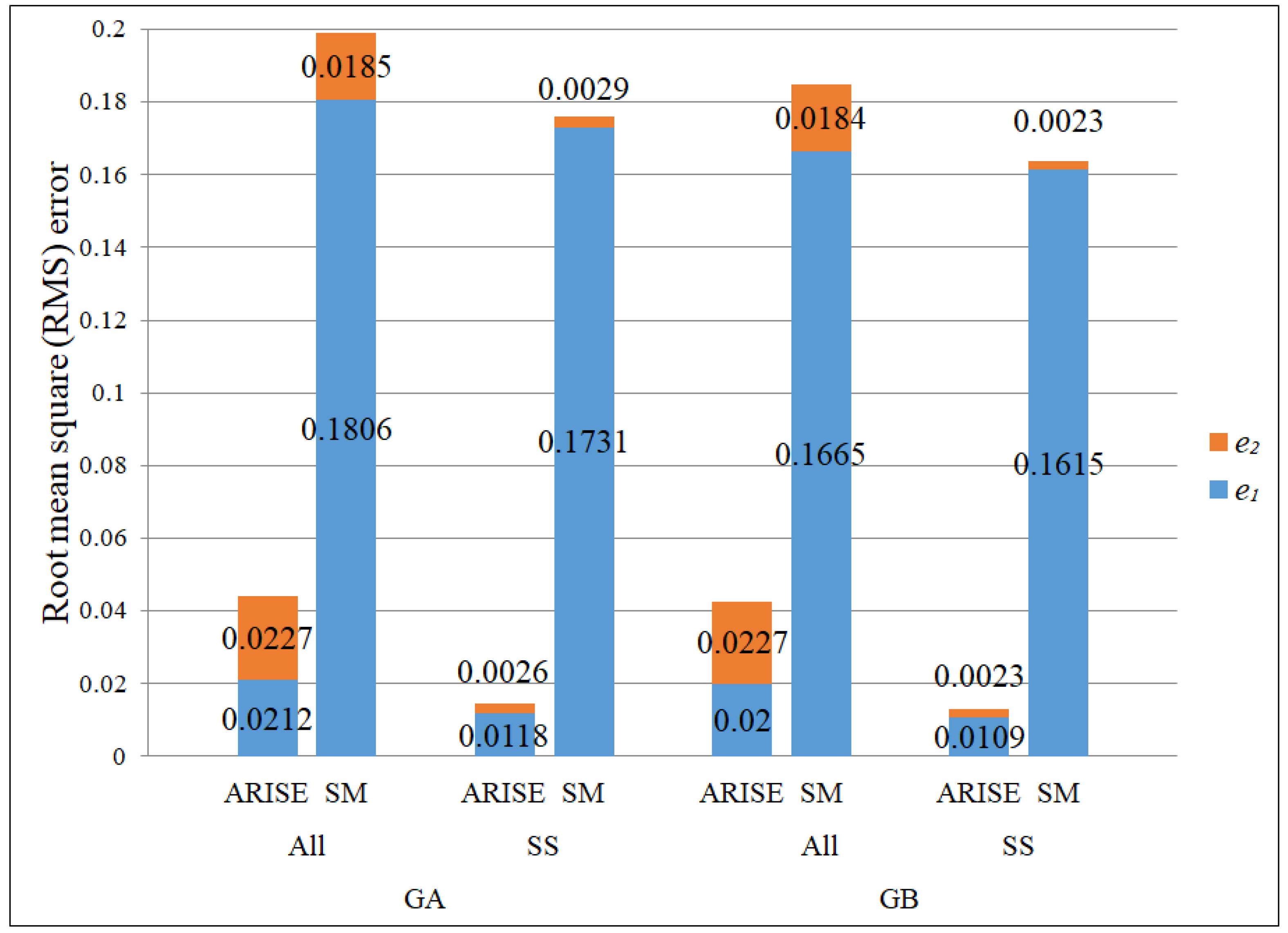
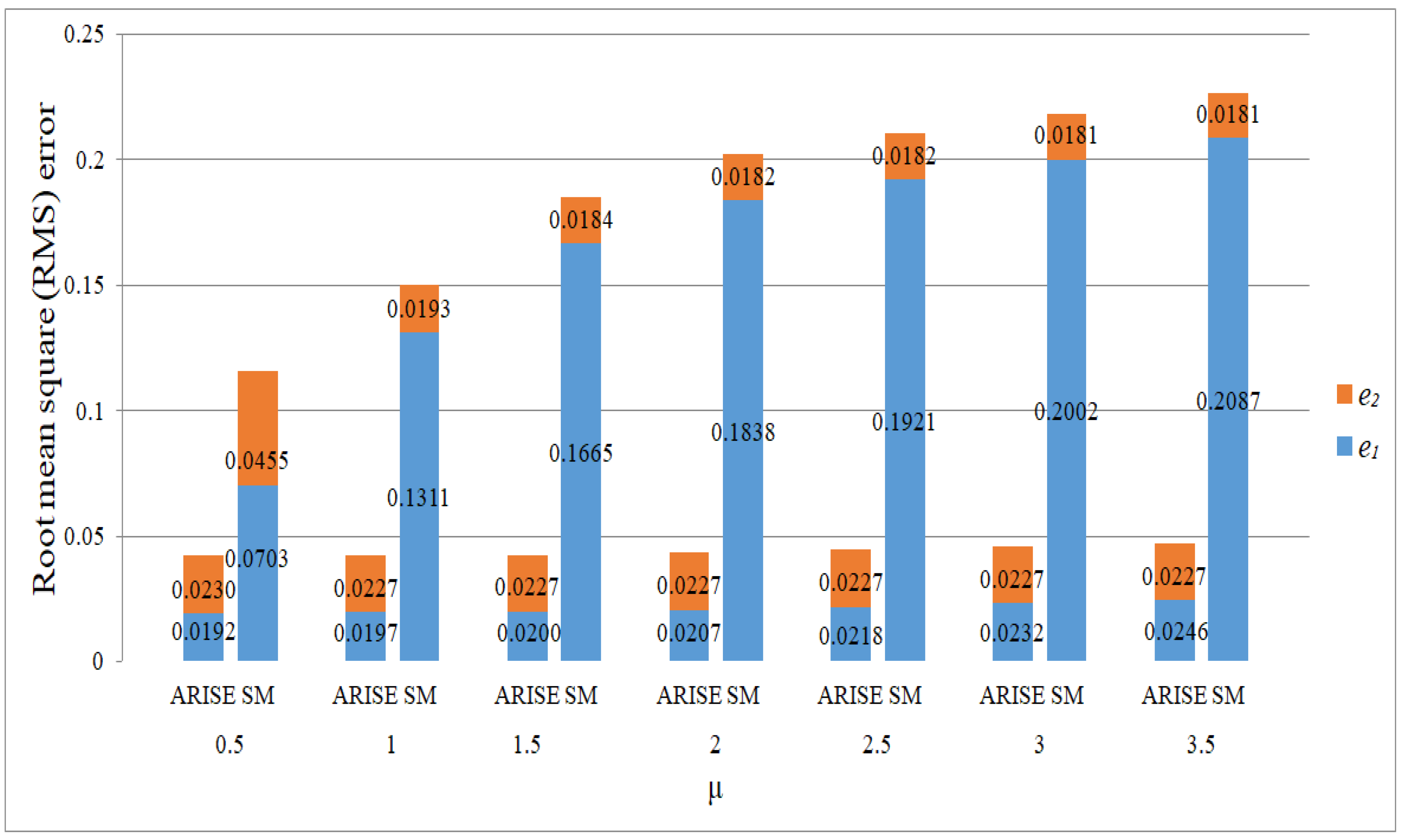
3. Results
4. Discussion
5. Conclusions
Author Contributions
Funding
Institutional Review Board Statement
Informed Consent Statement
Data Availability Statement
Conflicts of Interest
Abbreviations
| ARISE | Auxiliary robust integral of sign of the error |
| SM | Sliding mode |
| RISE | Robust integral of the sign of the error |
| RMS | Root mean square |
References
- Abdallah, C.; Dawson, D.; Dorato, P.; Jamshidi, M. Survey of robust control for rigid robots. IEEE Control Syst. Mag. 1991, 11, 24–30. [Google Scholar]
- Khalil, H.K. Nonlinear Systems, 3rd ed.; Prentice Hall: Upper Saddle River, NJ, USA, 2002. [Google Scholar]
- Allen, B.C.; Cousin, C.; Rouse, C.; Dixon, W.E. Cadence Tracking for Switched FES Cycling with Unknown Input Delay. In Proceedings of the IEEE 58th Conference on Decision and Control (CDC), Nice, France, 11–13 December 2019; pp. 60–65. [Google Scholar]
- Dixon, W.E.; Fang, Y.; Dawson, D.M.; Chen, J. Adaptive Range Identification for Exponential Visual Servo Control. In Proceedings of the IEEE International Symposium on Intelligent Control, Houston, TX, USA, 8 October 2003; pp. 46–51. [Google Scholar]
- Allen, B.; Stubbs, K.; Dixon, W.E. Data-Based and Opportunistic Integral Concurrent Learning for Adaptive Trajectory Tracking During Switched FES-Induced Biceps Curls. IEEE Trans. Neural Syst. Rehabil. Eng. 2022, 30, 2557–2566. [Google Scholar] [CrossRef] [PubMed]
- Duenas, V.; Cousin, C.A.; Ghanbari, V.; Fox, E.J.; Dixon, W.E. Torque and Cadence Tracking in Functional Electrical Stimulation Induced Cycling using Passivity-Based Spatial Repetitive Learning Control. Automatica 2020, 115, 108852. [Google Scholar] [CrossRef]
- Slotine, J.; Li, W. Applied Nonlinear Control; Prentice Hall: Upper Saddle River, NJ, USA, 1991. [Google Scholar]
- Kwan, C.M.; Dawson, D.M.; Lewis, F.L. Robust Adaptive Control of Robots Using Neural Network: Global Tracking Stability. In Proceedings of the IEEE Conference on Decision and Control, New Orleans, LA, USA, 13–15 December 1995; pp. 1846–1851. [Google Scholar]
- Ge, S.S.; Hang, C.C.; Woon, L.C. Adaptive Neural Network Control of Robot Manipulators in Task Space. IEEE Trans. Ind. Electron. 1997, 44, 746–752. [Google Scholar]
- Corradini, M.; Cristofaro, A.; Orlando, G. Robust Stabilization of Multi Input Plants with Saturating Actuators. IEEE Trans. Autom. Control 2010, 55, 419–425. [Google Scholar] [CrossRef]
- Patre, P.M.; Dupree, K.; MacKunis, W.; Dixon, W.E. A New Class of Modular Adaptive Controllers, Part II: Neural Network Extension for Non-LP Systems. In Proceedings of the 2008 American Control Conference, Seattle, WA, USA, 11–13 June 2008; pp. 1214–1219. [Google Scholar]
- Hu, G.; Dixon, W.E.; Ding, H. Robust Tracking Control of an Array of Nanoparticles Moving on a Substrate. Automatica 2012, 48, 442–448. [Google Scholar] [CrossRef]
- Patre, P.M.; MacKunis, W.; Kaiser, K.; Dixon, W.E. Asymptotic Tracking for Uncertain Dynamic Systems via a Multilayer Neural Network Feedforward and RISE Feedback Control Structure. IEEE Trans. Autom. Control 2008, 53, 2180–2185. [Google Scholar] [CrossRef]
- Cheng, T.H.; Downey, R.; Dixon, W.E. Robust output feedback control of uncertain switched Euler-Lagrange systems. In Proceedings of the IEEE Conference on Decision and Control, Firenze, Italy, 10–13 December 2013; pp. 4668–4673. [Google Scholar]
- Dixon, W.E.; Dawson, D.M.; Zergeroglu, E.; Behal, A. Adaptive Tracking Control of a Wheeled Mobile Robot via an Uncalibrated Camera System. IEEE Trans. Syst. Man Cybern. Part B Cybern. 2001, 31, 341–352. [Google Scholar] [CrossRef]
- Dixon, W.E.; Zergeroglu, E.; Dawson, D.M.; Hannan, M.W. Global Adaptive Partial State Feedback Tracking Control of Rigid-Link Flexible-Joint Robots. Robotica 2000, 18, 325–326. [Google Scholar] [CrossRef]
- Cheng, M.B.; Tsai, C.C. Hybrid Robust Tracking Control for a Mobile Manipulator via Sliding-Mode Neural Network. In Proceedings of the IEEE International Conference on Mechatronics, Taipei, Taiwan, 10–12 July 2005; pp. 537–542. [Google Scholar]
- Cousin, C.A.; Rouse, C.A.; Duenas, V.H.; Dixon, W.E. Controlling the Cadence and Admittance of a Functional Electrical Stimulation Cycle. IEEE Trans. Neural Syst. Rehabil. Eng. 2019, 27, 1181–1192. [Google Scholar] [CrossRef]
- Sun, R.; Greene, M.; Le, D.; Bell, Z.; Chowdhary, G.; Dixon, W.E. Lyapunov-Based Real-Time and Iterative Adjustment of Deep Neural Networks. IEEE Control Syst. Lett. 2022, 6, 193–198. [Google Scholar] [CrossRef]
- Komurcugil, H.; Biricik, S.; Bayhan, S.; Zhang, Z. Sliding Mode Control: Overview of Its Applications in Power Converters. IEEE Ind. Electron. Mag. 2021, 15, 40–49. [Google Scholar] [CrossRef]
- Rojas, L.; Yepes, V.; Garcia, J. Complex Dynamics and Intelligent Control: Advances, Challenges, and Applications in Mining and Industrial Processes. Mathematics 2025, 13, 961. [Google Scholar] [CrossRef]
- Dixon, W.E.; Fang, Y.; Dawson, D.M.; Flynn, T.J. Range Identification for Perspective Vision Systems. IEEE Trans. Autom. Control 2003, 48, 2232–2238. [Google Scholar] [CrossRef]
- Dinh, H.T.; Kamalapurkar, R.; Bhasin, S.; Dixon, W.E. Dynamic Neural Network-based Robust Observers for Uncertain Nonlinear Systems. Neural Netw. 2014, 60, 44–52. [Google Scholar] [CrossRef]
- Fischer, N.; Kamalapurkar, R.; Sharma, N.; Dixon, W.E. RISE-Based Control of an Uncertain Nonlinear System with Time-Varying State Delays. In Proceedings of the IEEE Conference on Decision and Control (CDC), Maui, HI, USA, 10–13 December 2012; pp. 3502–3507. [Google Scholar]
- Hiramatsu, T.; Johnson, M.; Fitz-Coy, N.; Dixon, W.E. Asymptotic Optimal Tracking Control for an Uncertain Nonlinear Euler-Lagrange System: A RISE-based Closed-Loop Stackelberg Game Approach. In Proceedings of the IEEE Conference on Decision and Control and European Control Conference, Orlando, FL, USA, 12–15 December 2011; pp. 1030–1035. [Google Scholar]
- Kamalapurkar, R.; Bialy, B.; Andrews, L.; Dixon, W.E. Adaptive RISE Feedback Control Strategies for Systems with Structured and Unstructured Uncertainties. In Proceedings of the AIAA Guidance, Navigation, and Control (GNC) Conference, Boston, MA, USA,, 19–22 August 2013. [Google Scholar]
- Sun, C.; Ye, M.; Hu, G. Distributed time-varying quadratic optimization for multiple agents under undirected graphs. IEEE Trans. Autom. Control 2017, 62, 3687–3694. [Google Scholar] [CrossRef]
- Stegath, K.; Sharma, N.; Gregory, C.; Dixon, W.E. Experimental Demonstration of RISE-Based NMES of Human Quadriceps Muscle. In Proceedings of the IEEE/NIH Life Science Systems and Applications Workshop, Bethesda, MD, USA, 8–9 November 2007; pp. 43–46. [Google Scholar]
- Isaly, A.; Patil, O.S.; Sweatland, H.M.; Sanfelice, R.G.; Dixon, W.E. Adaptive Safety with a RISE-Based Disturbance Observer. IEEE Trans. Autom. Control 2024, 69, 4883–4890. [Google Scholar] [CrossRef]
- Cai, Z.; de Queiroz, M.S.; Dawson, D.M. Robust adaptive asymptotic tracking of nonlinear systems with additive disturbance. IEEE Trans. Autom. Control 2006, 51, 524–529. [Google Scholar] [CrossRef]
- Makkar, C.; Hu, G.; Sawyer, W.G.; Dixon, W.E. Lyapunov-Based Tracking Control in the Presence of Uncertain Nonlinear Parameterizable Friction. IEEE Trans. Autom. Control 2007, 52, 1988–1994. [Google Scholar] [CrossRef]
- Patre, P.; Bhasin, S.; Wilcox, Z.D.; Dixon, W.E. Composite Adaptation for Neural Network-Based Controllers. IEEE Trans. Autom. Control 2010, 55, 944–950. [Google Scholar] [CrossRef]
- Patre, P.M.; MacKunis, W.; Dupree, K.; Dixon, W.E. RISE-Based Robust and Adaptive Control of Nonlinear Systems; Birkhauser: Boston, MA, USA, 2010. [Google Scholar]
- Sharma, N.; Bhasin, S.; Wang, Q.; Dixon, W.E. RISE-Based Adaptive Control of a Control Affine Uncertain Nonlinear System with Unknown State Delays. IEEE Trans. Autom. Control 2012, 57, 255–259. [Google Scholar] [CrossRef]
- Zhao, B.; Xian, B.; Zhang, Y.; Zhang, X. Nonlinear robust adaptive tracking control of a quadrotor UAV via immersion and invariance methodology. IEEE Trans. Ind. Electron. 2014, 62, 2891–2902. [Google Scholar] [CrossRef]
- Patre, P.M.; Mackunis, W.; Makkar, C.; Dixon, W.E. Asymptotic Tracking for Systems with Structured and Unstructured Uncertainties. IEEE Trans. Control Syst. Technol. 2008, 16, 373–379. [Google Scholar] [CrossRef]
- Qu, Z.; Xu, J.X. Model-Based Learning Controls And Their Comparisons Using Lyapunov Direct Method. Asian J. Control 2002, 4, 99–110. [Google Scholar] [CrossRef]
- Yang, G.; Zhu, T.; Yang, F.; Cui, L.; Wang, H. Output feedback adaptive RISE control for uncertain nonlinear systems. Asian J. Control 2023, 25, 433–442. [Google Scholar] [CrossRef]
- Patil, O.; Isaly, A.; Xian, B.; Dixon, W.E. Exponential Stability with RISE Controllers. IEEE Control Syst. Lett. 2022, 6, 1592–1597. [Google Scholar] [CrossRef]
- Ting, J.; Basyal, S.; Allen, B.C. Robust Control of a Nonsmooth or Switched Control Affine Uncertain Nonlinear System Using a Novel RISE-Inspired Approach. In Proceedings of the American Control Conference (ACC), San Diego, CA, USA, 31 May–2 June 2023. [Google Scholar]
- Cai, Z.; de Queiroz, M.S.; Dawson, D.M. A sufficiently smooth projection operator. IEEE Trans. Autom. Control 2006, 51, 135–139. [Google Scholar] [CrossRef]
- Filippov, A.F. Differential equations with discontinuous right-hand side. In Fifteen Papers on Differential Equations; American Mathematical Society Translations—Series 2; American Mathematical Society: Providence, RI, USA, 1964; Volume 42, pp. 199–231. [Google Scholar]
- Paden, B.E.; Sastry, S.S. A calculus for computing Filippov’s differential inclusion with application to the variable structure control of robot manipulators. IEEE Trans. Circuits Syst. 1987, 34, 73–82. [Google Scholar] [CrossRef]


| Disturbances | ||
|---|---|---|
| a | 0.5cos(t) | 0.5sin(t) |
| b | 0.1cos(t) | 0.1sin(t) |
| c | 0.05cos(t) | 0.05sin(t) |
| d | 0.01cos(t) | 0.01sin(t) |
| e | 0.5 | 0.5 |
| f | 0.1 | 0.1 |
| g | 0.05 | 0.05 |
| h | 0.01 | 0.01 |
Disclaimer/Publisher’s Note: The statements, opinions and data contained in all publications are solely those of the individual author(s) and contributor(s) and not of MDPI and/or the editor(s). MDPI and/or the editor(s) disclaim responsibility for any injury to people or property resulting from any ideas, methods, instructions or products referred to in the content. |
© 2025 by the authors. Licensee MDPI, Basel, Switzerland. This article is an open access article distributed under the terms and conditions of the Creative Commons Attribution (CC BY) license (https://creativecommons.org/licenses/by/4.0/).
Share and Cite
Basyal, S.; Ting, J.; Mishra, K.; Allen, B.C. The Robust Control of a Nonsmooth or Switched Control-Affine Uncertain Nonlinear System Using an Auxiliary Robust Integral of the Sign of the Error (ARISE) Controller. Appl. Sci. 2025, 15, 4482. https://doi.org/10.3390/app15084482
Basyal S, Ting J, Mishra K, Allen BC. The Robust Control of a Nonsmooth or Switched Control-Affine Uncertain Nonlinear System Using an Auxiliary Robust Integral of the Sign of the Error (ARISE) Controller. Applied Sciences. 2025; 15(8):4482. https://doi.org/10.3390/app15084482
Chicago/Turabian StyleBasyal, Sujata, Jonathan Ting, Kislaya Mishra, and Brendon Connor Allen. 2025. "The Robust Control of a Nonsmooth or Switched Control-Affine Uncertain Nonlinear System Using an Auxiliary Robust Integral of the Sign of the Error (ARISE) Controller" Applied Sciences 15, no. 8: 4482. https://doi.org/10.3390/app15084482
APA StyleBasyal, S., Ting, J., Mishra, K., & Allen, B. C. (2025). The Robust Control of a Nonsmooth or Switched Control-Affine Uncertain Nonlinear System Using an Auxiliary Robust Integral of the Sign of the Error (ARISE) Controller. Applied Sciences, 15(8), 4482. https://doi.org/10.3390/app15084482