Optical Flow Odometry with Panoramic Image Based on Spherical Congruence Projection

Abstract

Panoramic images provide distinct advantages in odometry applications, which are largely due to their extensive field of view and higher information density captured in a single frame. Traditional odometry methods often rely on mapping panoramic images onto the planar structure for feature tracking. However, this process introduces uneven distortions of features, which diminish the accuracy of feature tracking and odometry, particularly in scenarios involving large displacements. In this work, we address this challenge by introducing a novel approach, named spherical congruence projection (SCP), that maps panoramic images onto a spherical structure and projects the spherical pixels onto a two-dimensional data format while preserving the spherical pixel topology. SCP effectively eliminates the distortion across the panoramic image. Additionally, we present the optical flow odometry on the panoramic image in the spherical structure and integrate it with the proposed SCP method for the first time. The experimental results in public and custom-built datasets demonstrate that the proposed SCP-based odometry method reliably tracks features and maintains accurate odometry performance, even in fast-moving scenarios.

1. Introduction

Panoramic images offer significant advantages in robotics, autonomous driving, and virtual reality due to their extensive field of view (FoV) [1,2,3]. In visual odometry, their panoramic nature allows for capturing comprehensive environmental information in a single frame, increasing the feature residence time within the sensor’s FoV. This higher information density enhances the accuracy and robustness of visual odometry systems [4].

However, utilizing panoramic images for feature-based odometry poses challenges, particularly in achieving continuous and undistorted feature extraction and tracking across a wide FoV. Original panoramic images suffer from serious image distortions, especially in the polar areas. Existing methods often rely on projecting panoramic images onto specific structures for feature processing, which are categorized into single-plane and multi-plane projection approaches. Single-plane projection methods map panoramic images onto a planar structure. For instance, Scaramuzza et al. [5] developed a model for catadioptric and fisheye cameras, which was later extended by Chen et al. [6] for panoramic annular lens (PAL) cameras. Ji et al. [7] employed equirectangular projection (ERP) to process panoramic images. Multi-plane projection methods divide the image into multiple planes with different viewpoints. Wang et al. [8], for example, proposed a cube map structure for fisheye cameras accompanied by a SLAM system. These methods significantly influence feature tracking accuracy, as shown in Figure 1.

Single-plane projections introduce region-dependent distortions, which lead to tracking inconsistencies, especially under fast motion where feature points experience significant displacements. While multi-plane projections reduce some distortion-related issues, they introduce data discontinuities and retain localized distortions, limiting their robustness under large pixel shifts.

To address these challenges, this paper proposes an optical flow odometry method based on a novel spherical congruence projection (SCP). Unlike the equirectangular projection, which introduces significant pixel stretching near the polar regions and exhibits nonlinear geometric distortion with increasing latitude, the SCP method ensures strict scale consistency across the spherical domain. Compared to multi-plane projection approaches, which often suffer from seam discontinuities and localized distortions at plane boundaries, SCP maintains topological and geometric continuity over the entire field of view. This distortion-free mapping enables smooth and consistent pixel tracking, even under fast motion and large displacements.

In addition, the proposed method integrates a spherical pixel structure with an optical flow tracking framework, allowing for fast and accurate feature association between frames. This dual capability—global distortion elimination and dense, robust tracking—ensures that the proposed system meets both the accuracy and efficiency requirements of panoramic image odometry in real-world scenarios.

The main contributions of this paper are summarized as follows:

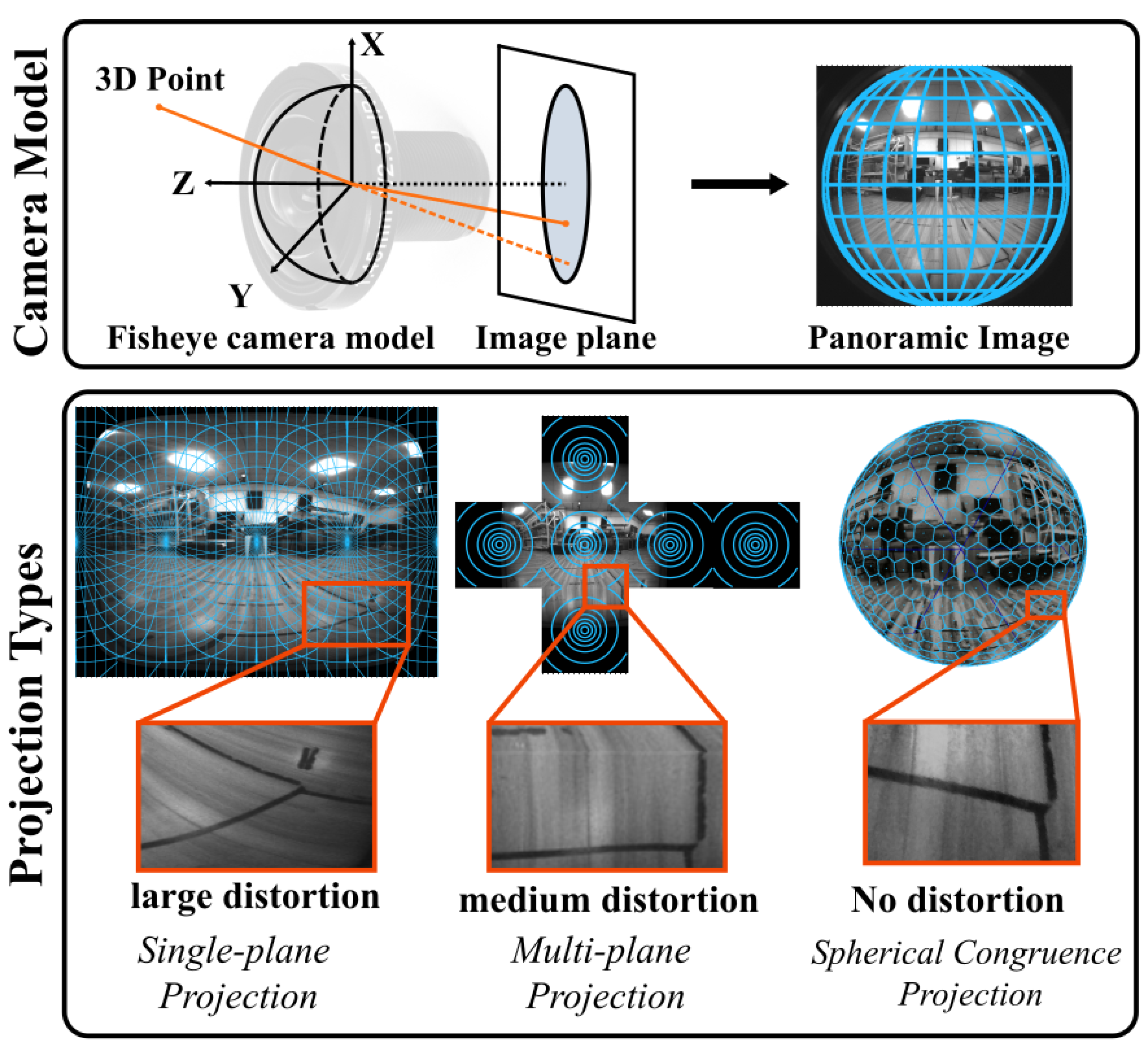
• We propose a spherical congruence projection method that provides a globally consistent, distortion-free representation of panoramic images. Unlike traditional ERP or multi-plane projections, SCP preserves pixel-wise scale and topology on the spherical surface, offering a unified and geometry-preserving alternative for downstream tracking tasks.
• We introduce a dense optical flow tracking framework tailored for spherical imagery. To the best of our knowledge, this is the first system to perform dense pixel–motion estimation directly on a spherical pixel structure. Our method integrates a nonorthogonal gradient operator specifically adapted to the sphere, enabling smooth and spatially consistent flow fields over the entire 360° FoV.
• We present a fully integrated visual odometry pipeline that combines spherical projection and dense flow tracking into a real-time system. Extensive experiments on both public and custom datasets demonstrate that our method not only achieves superior accuracy under high-speed motion but also offers improved robustness compared to existing fisheye and panoramic odometry methods.

The rest of this paper is organized as follows. In Section 2, a brief review of odometry algorithms based on panoramic images is given. Section 3 presents the details of the proposed SCP method, and the experiments are conducted and analyzed in Section 4. Section 5 concludes the paper.

2. Related Work

2.1. Panoramic Image-Based Feature Tracking

In response to the varying distortion ratios across the panoramic images, researchers have proposed various strategies to mitigate its impact on feature tracking, as well as the SLAM system. The most straightforward approach is employing feature tracking algorithms designed for planar perspective images on untreated panoramic images directly [9]. However, the extracted feature point and its associated neighborhoods required for optical flow calculations undergo varying degrees of distortion, adversely affecting matching accuracy. Seok et al. [10] addressed the distortion issue by performing feature tracking in areas with slight distortion, although this approach sacrifices the advantage of the panoramic image, which is the broad field of view.

One commonly used approach to distortion correction involves projecting the original panoramic image into different formats and eliminating the distortion during the projection process. Youngho Yoon et al. [11] represented the panoramic image as a subdivided icosahedron and proposed a framework to reconstruct a low-resolution 360° image to a high-resolution image. To apply the convolutional neural network to spherical images, Yeonkun Lee et al. [12] proposed an approach by utilizing the spherical polyhedron to represent omnidirectional images. Xu Gao et al. [13] presented an optimized content-aware projection method to alleviate the distortion problem during depth estimation of 360° images. Aguiar et al. [14] utilized the Scaramuzza model to rectify the panoramic image into the planar perspective image to eliminate image distortion. Wang et al. [8] suggested projecting the panoramic image onto a cube by treating each cube face as an image plane of a virtual pinhole camera with 90° FoV. Lee et al. [15] extended this approach by combining the Enhanced Unified Camera Mode during the cube map. Besides the cube shape, some researchers tried to project the panoramic image onto a polyhedron to mitigate pixel distortion [16]. While the image is corrected for individual planes, noticeable pixel stretching or compressing near the corners and edges is inevitable for the cube and polyhedron images, and the continuous flow of information in panoramic images is disrupted as well.

Another widely used projection method is ERP, which maps the spherical image onto the 2D plane based on the longitude and latitude coordinates of pixels [17]. However, ERP images suffer from poor pixel uniformity, resulting in significant information loss when projecting content near the poles. Therefore, even though ERP-based feature tracking offers computational efficiency, it is suboptimal in terms of matching accuracy.

To address the issue of uneven pixel distribution in ERP images, Kitamura et al. [18] adopted the geodesic grid-based spherical data structure for panoramic images, which was developed by Williamson [19], and proposed an FAST corner feature extraction method utilizing this structure. This approach achieved better pixel uniformity compared to longitude–latitude-based segmentation. Zhao et al. [20] introduced the SPHORB algorithm for panoramic images based on a similar geodesic grid segmentation approach, which outperformed the traditional ORB algorithm for panoramic images in tasks of feature tracking. Guan et al. [21] proposed the BRISKS feature for spherical images on a geodesic grid. Compared to SPHORB, the statistical-based feature extraction approach makes it more adaptable to varying pixel structures, albeit with a tradeoff in extraction efficiency. Studies in [22,23] attempted to represent the distortion information using an attitude matrix and built a distorted Binary Robust Independent Elementary Feature (BRIEF) descriptor for the fisheye camera. Christiano et al. [24] and Javier et al. [25] proposed methods involving projecting the spherical pixel and its surroundings onto the tangent plane and constructing the descriptor accordingly. However, these approaches introduce the additional computational burden of calculating the tangent plane, thereby reducing the overall efficiency of the feature tracking process.

2.2. Panoramic Image-Based Odometry

Recent years have witnessed a growing interest in using panoramic images for odometry and SLAM tasks, owing to their wide field of view (FoV) and the advantage of long-term feature visibility across frames. A variety of methods have been developed to exploit this modality, which can be roughly categorized into visual-only, LiDAR-assisted (VLO), and visual–inertial (VIO) approaches.

One of the earlier works in this domain is ROVO [10], which employs multiple panoramic cameras with overlapping FoVs to improve pose estimation accuracy by enhancing feature redundancy. More recently, 360ORB-SLAM [26] proposed a monocular SLAM system tailored for panoramic cameras, combining traditional ORB-based sparse feature tracking with a depth completion network. This design significantly improves both scale estimation and robustness under challenging visual conditions.

Several methods have focused on integrating panoramic vision with LiDAR data to enhance robustness and geometric consistency. LF-VISLAM [27] incorporates panoramic imagery and LiDAR input into the LVI-SAM framework, extending the backend optimization and loop closure capabilities. Panoramic direct LiDAR-assisted VO [28] further establishes geometric alignment between panoramic images and 360° LiDAR point clouds, demonstrating improved pose estimation under sparse features or rapid motion.

To improve performance in dynamic scenes or under aggressive motion, visual–inertial fusion has also been explored. ROVINS [29], an extension of ROVO, introduces IMU constraints into the panoramic visual pipeline to enhance motion estimation stability. Wang et al. [30] proposed a real-time VIO framework that robustly handles feature tracking even in the negative hemisphere of panoramic images. More recently, PAL-SLAM2 [31] has been used to map panoramic image features onto a unit sphere and perform tightly coupled visual–inertial bundle adjustment in the spherical domain, providing improved accuracy and loop closure performance.

Although the aforementioned systems leverage panoramic imagery for odometry and SLAM, they often rely on conventional projection models such as equirectangular projection or image stitching, which introduce severe distortions near the poles or discontinuities across seams. Moreover, most methods are built upon sparse feature-based matching pipelines, which suffer from inconsistency in motion estimation under large pixel shifts or dynamic scenes. In contrast, our method introduces a dense optical flow-based odometry framework built directly on a distortion-free spherical pixel structure. This enables continuous, pixel-wise tracking across the full FoV and offers a new perspective for robust full-view visual odometry in panoramic scenarios.

3. Materials and Methods

Figure 2 illustrates the structure of the proposed SCP optical flow odometry method, which contains three parts. First, the raw panoramic image is converted into a three-dimensional spherical structure through spherical mapping, and the pixels in the corresponding spherical image are evenly segmented. Then, the spherical image is divided into six subregions of equal area according to the pixel distribution. Eventually, the gradient of pixels within each subregion is calculated, followed by optical flow tracking based on these gradients.

3.1. Spherical Mapping and Pixelation

Consider a pixel in the panoramic image $\mathcal{S}$ with the coordinate denoted as $P_c$, where its corresponding point in world coordinate is represented as $P_w$, as shown in Figure 3. Due to the unique imaging characteristics of panoramic cameras, the traditional pinhole camera model can not accurately represent the translation between $P_c$ and $P_w$. In this paper, the omnidirectional camera model proposed by Davide Scaramuzza [32] is adopted to describe the relationship between the point $P_c$ and the vector ${\mathbf{p}}_w$ emanating from the viewpoint. By normalizing the incident light vectors for all pixels, the panoramic image $\mathcal{S}$ in the planar structure can be transformed into a spherical image ${\mathcal{S}}^{\prime }$. In this spherical structure, the spatial coordinate of the corresponding pixel point within the viewpoint coordinate system is $P_c^{\prime }={\mathbf{p}}_w/∥{\mathbf{p}}_w∥=\left\{x,y,z\right\}$.

Conducting optical flow on the spherical-structure image ${\mathcal{S}}^{\prime }$ directly presents significant challenges due to its varying pixel density and the complexity of motion patterns on the spherical surface. To overcome the above issue, the Quasi-Uniform Voronoi Sphere (QUVS) strategy [33] is employed to resample the pixels of ${\mathcal{S}}^{\prime }$ uniformly. Specifically, the QUVS is an icosahedron-based spherical homogenization method, which conducts iterative refinement using the Voronoi algorithm. The vertices are treated as electrons in QUVS, and the uniform pixel distribution is achieved through electrostatic repulsion balance. Then, the pixel grids are generated according to those vertices. Owing to the intrinsic properties of the icosahedron, the pixel grids contain two types: hexagonal pixels and pentagonal pixels. Denote the QUVS image as ${\tilde{\mathcal{S}}}_L$, whose refinement level is L. The corresponding number of pixels in ${\tilde{\mathcal{S}}}_L$ is $N_L$, of which 12 are pentagonal pixels, and the remaining $N_L-12$ pixels are hexagonal pixels. The QUVS image ${\tilde{\mathcal{S}}}_L$ maintains geometric consistency across the entire view, eliminating the feature distortion of pixels in the associated 2D planar image.

3.2. Spherical Congruence Projection

The pixels of ${\tilde{\mathcal{S}}}_L$ are arranged within the 3D space, which presents challenges for storage and memory management, as well as incurs higher computational load. To optimize pixel storage in the computer, we propose a strategy to project spherical pixels onto the 2D plane, referred to as the spherical congruence projection, while preserving topological consistency. The procedure of SCP includes two stages, spherical pixel segmentation and pixel storage, with the corresponding flowchart shown in Figure 4.

3.2.1. Spherical Pixel Segmentation

For the QUVS image, the number of twelve pentagonal pixels remains constant. These pentagonal pixels are uniformly distributed across the six directional axes of the pole pixel. According to the distribution characteristics of pentagonal pixels, the entire spherical pixel space can be partitioned into six distinct subregions. With the north origin pixel $O_N$ and the south origin pixel $O_S$ of ${\tilde{\mathcal{S}}}_L$, two hexagonal coordinate systems can be constructed with axes ${\omega }_N^1$ to ${\omega }_N^6$ and ${\omega }_S^1$ to ${\omega }_S^6$ separately, as shown in Figure 5, where ${\omega }_N^1$ though ${\omega }_N^6$ correspond to the directional vectors from $O_N$, and ${\omega }_S^1$ though ${\omega }_S^6$ correspond to the directional vectors from $O_S$. For each coordinate system, the direction of each axis points to the center of the adjacent hexagonal pixel. The following outlines the construction of the boundary pixels for the spherical segmentation area.

In the first step, the boundary pixels begin at $O_N$, extend along each axis until reaching the encountered pentagonal pixel, and repeat the above process in the same manner from $O_S$. The second step begins with the pentagonal pixels encountered in the previous step. For the pentagonal pixels extending from $O_N$, the boundary pixels are further extended to the lower left. For the pentagonal pixels extending from $O_S$, the boundary pixels are further extended to the upper right until the two groups of pixels intersect. The boundary pixels effectively partition ${\tilde{\mathcal{S}}}_L$ into six distinct subregions. By cropping along the boundary pixels and flatting pixels, six 2D images $\left\{\widetilde{{\mathcal{S}}_{\mathcal{C}}}\right|C=1,\cdots ,6\}$ can be generated that preserve the topological relationships of the spherical pixels, as shown in the bottom row of Figure 5. To ensure that each subregion includes its own boundary area, the boundary pixels used for segmentation are duplicated across adjacent subregions. This duplication allows each subregion to maintain a clear boundary, facilitating independent processing or analysis.

3.2.2. Pixel Storage

To facilitate pixel storage and calculation in physical memory, which usually contains the linear layout, the pixels in subregions with hexagonal coordinates are transferred to the Cartesian coordinate system. According to the pixel distribution of each subregion, they can be divided into two categories, where subregions in quadrants $\left\{{\omega }_N^1,{\omega }_N^2\right\}$, $\left\{{\omega }_N^3,{\omega }_N^4\right\}$, and $\left\{{\omega }_N^5,{\omega }_N^6\right\}$ are regarded as Right-leaning Region (RR) ${\tilde{\mathcal{S}}}_{RR}$, while subregions in quadrants $\left\{{\omega }_N^2,{\omega }_N^3\right\}$, $\left\{{\omega }_N^4,{\omega }_N^5\right\}$, and $\left\{{\omega }_N^6,{\omega }_N^1\right\}$ form Left-leaning Region (LR) ${\tilde{\mathcal{S}}}_{LR}$. In each subregion, the pixels are indexed according to their centroid coordinates $(x,y)$ along the axes, where x and y represent indices along the ${\omega }_N^x$ and ${\omega }_N^y$ axes, respectively. Note that the origins for ${\tilde{\mathcal{S}}}_{RR}$ and ${\tilde{\mathcal{S}}}_{LR}$ are located at $O_N$. As shown in Figure 6, these pixel indices in the hexagonal coordinate are transformed into the Cartesian coordinate while maintaining the topological structure of pixels, i.e., $\left(x,y\right)⟹\left(u,v\right)$, where u and v denote the corresponding positions of x and y in the Cartesian coordinate. The transformed output, denoted as $\mathcal{G}$, represents the final SCP image. Since the typology structure between ${\tilde{\mathcal{S}}}_L$ and $\mathcal{G}$ remains unchanged, u and v are typically consistent with x and y.

After the transformation, the height H and width W of $\mathcal{G}$ are given as follows:

$$H=2\ast \left(2^{{\displaystyle \frac{L-1}{2}}}+1\right)-1$$

(1)

$$W=3\ast \left(2^{{\displaystyle \frac{L-1}{2}}}+1\right)-2$$

(2)

where L represents the refinement level of the original QUVS image ${\tilde{\mathcal{S}}}_L$. Taking the north pole $O_N$ as the origin, the coordinates of pentagonal pixels $\left\{p_{RR}^1,p_{RR}^2,p_{RR}^3,p_{RR}^4\right\}$ in ${\tilde{\mathcal{S}}}_{RR}$ are located at $\left(0,{\displaystyle \frac{H-1}{2}}\right)$, $\left({\displaystyle \frac{W-1}{3}},H-1\right)$, $\left(W-1,{\displaystyle \frac{H-1}{2}}\right)$, $\left({\displaystyle \frac{2(W-1)}{3}},0\right)$, respectively. Similarly, the positions of pentagonal pixels $\left\{p_{LR}^1,p_{LR}^2,p_{LR}^3,p_{LR}^4\right\}$ in ${\tilde{\mathcal{S}}}_{LR}$ are $\left(0,{\displaystyle \frac{H-1}{2}}\right)$, $\left({\displaystyle \frac{2(W-1)}{3}},0\right)$, $\left(W-1,{\displaystyle \frac{H-1}{2}}\right)$, and $\left({\displaystyle \frac{W-1}{3}},H-1\right)$. As mentioned above, the boundary pixels of adjacent ${\tilde{\mathcal{S}}}_{RR}$ and ${\tilde{\mathcal{S}}}_{LR}$ are shared. Taking the pentagonal pixels in Figure 6 as the example, $p_{RR}^4$ and $p_{RR}^3$ on the boundary of ${\tilde{\mathcal{S}}}_{RR}$ correspond to the $p_{LR}^2$ and $p_{LR}^3$ in ${\tilde{\mathcal{S}}}_{LR}$.

3.3. SCP-VO Method

With the advantages of the SCP images, an SCP-based Visual Odometry (SCP-VO) is proposed accordingly. The SCP-VO leverages the optical flow principles to accurately identify and track features on the projected SCP images.

$${\mathrm{H}}_7^v={\mathrm{H}}_7^u+{\mathrm{H}}_7^m$$

(3)

$${\mathrm{H}}_7^u=\left[\begin{array}{cccc}& -a& & +a\\ -b& & 0& & +b\\ & -a& & +a\end{array}\right]$$

(4)

$${\mathrm{H}}_7^v=\left[\begin{array}{cccc}& -b& & -a\\ -a& & 0& & +a\\ & +a& & +b\end{array}\right]$$

(5)

$${\mathrm{H}}_7^m=\left[\begin{array}{ccccc}& -a& & -b& \\ +a& & 0& & -a\\ & +b& & +a\end{array}\right]$$

(6)

On planar images, gradient operators are typically constructed along two orthogonal and independent directions—horizontal and vertical. In contrast, the QUVS pixel structure employed in this work is defined over a spherical domain and is characterized by three symmetric axes, denoted as u, v, and m, which are rotationally related by 60 degrees. Due to the inherently two-dimensional nature of the spherical surface, these three axes are geometrically coupled rather than mutually independent.

Let $H_7^u$, $H_7^v$, and $H_7^m$ represent the discrete gradient operators along the u, v, and m directions, respectively. Their mutual spatial constraints are described in Equation (3). Based on the rotational symmetry of the QUVS structure, we construct three directional gradient operators using six sampling directions—$[-v,-m,u,v,m,-u]$—as shown in Equations (4)–(6). These directions correspond to pixel indices #1 through #6 illustrated in Figure 7.

By jointly considering the spatial constraint relationship in Equation (3) and the gradient formulation in Equation (4), we derive the following parameter constraint in the gradient operator:

$$b=2a$$

(7)

To estimate camera motion by minimizing photometric error, it is essential to compute pixel-wise gradients for tracking feature displacements across consecutive frames. In our framework, we select the u and v axes as two independent directions for gradient computation and consider both RR and LR cases. Specifically, the gradient operator in u and v directions for ${\tilde{\mathcal{S}}}_{RR}$ are

$$G_u^{RR}=\left[\begin{array}{ccc}0& -a& a\\ -b& 0& b\\ -a& a& 0\end{array}\right]$$

(8)

$$G_v^{RR}=\left[\begin{array}{ccc}0& -b& -a\\ -a& 0& a\\ a& b& 0\end{array}\right]$$

(9)

The gradient operator for u and v directions in ${\tilde{\mathcal{S}}}_{LR}$ are calculated as

$$G_u^{LR}=\left[\begin{array}{ccc}-a& a& 0\\ -b& 0& b\\ 0& -a& a\end{array}\right]$$

(10)

$$G_v^{LR}=\left[\begin{array}{ccc}-b& -a& 0\\ -a& 0& a\\ 0& a& b\end{array}\right]$$

(11)

Generally, neighboring pixels within the integration window are assumed to exhibit consistent motion. Thus, the pixel velocity can be characterized by the vector $\overline{\eta }$ that minimizes the photometric error across all pixels within the integration window. This minimization can be efficiently achieved using a one-step computation as follows:

$$\overline{\eta }=G^{-1}\overline{b}$$

(12)

where $\overline{b}$ represents the image mismatch vector, and G denotes the spatial gradient matrix and is defined below. Let the width and height of the associated integration window be $(2\ast w_u+1)\times (2\ast w_v+1)$. Then, the calculation of G and $\overline{b}$ can be expressed as

$$G=\sum _{u=p_u-w_u}^{p_u+w_u}\sum _{v=p_v-w_v}^{p_v+w_v}\left[\begin{array}{cc}{G}_u^2(u,v)& G_u(u,v)G_v(u,v)\\ G_u(u,v)G_v(u,v)& G_v^2(u,v)\end{array}\right]$$

(13)

$$\overline{b}=\sum _{u=p_u-w_u}^{p_u+w_u}\sum _{v=p_v-w_v}^{p_v+w_v}\left[\begin{array}{c}\delta I(u,v)·G_u(u,v)\\ \delta I(u,v)·G_v(u,v)\end{array}\right]$$

(14)

where $\delta I(u,v)$ represents the intensity difference between the adjacent images at the position $(u,v)$. Eventually, the prediction of the feature pixel in the next frame can be predicted as below. According to the matched feature points between consecutive frames, the camera’s motion can be estimated by minimizing the photometric error.

$${(u,v)}_k={(u,v)}_{k-1}+\overline{\eta }$$

(15)

As the spherical image ${\tilde{\mathcal{S}}}_L$ is divided into six subregions, the feature points may shift between regions, leading to the “cross-domain” phenomenon, particularly near the north and south poles where subregions intersect. Assume that the coordinate of the feature point in the subregion ${\tilde{\mathcal{S}}}_{RR1}$ is $\left(u_t,v_t\right)$ at time t, and the predicted coordinate can be calculated as $\left(u_{t+1},v_{t+1}\right)$ based on Equation (15). If $\left(u_{t+1},v_{t+1}\right)$ exceeds the boundary of ${\tilde{\mathcal{S}}}_{RR1}$, the corresponding spherical coordinate $\tilde{P}$ in ${\tilde{\mathcal{S}}}_L$ can be calculated based on the Scaramuzza camera model. Then, project $\tilde{P}$ onto the SCP image, and identify in which subregion the projected pixel resides. The projected pixel represents the location of $\left(u_{t+1},v_{t+1}\right)$ after “cross-domain” and participates in optical flow tracking with the newly extracted feature points in the next frame. As the pixel correspondence between ${\tilde{\mathcal{S}}}_L$ and subregions remains fixed, a link table can be generated in the preprocessing stage and retrieved during the practical stage. This approach eliminates the motion prediction procedure when exceeded pixels cross the subregion boundary, thereby enhancing the efficiency of tracking such boundary-crossing pixels.

3.4. Integration with Inertial Odometry

As illustrated in Figure 8, the proposed SCP-VO framework can be seamlessly integrated with inertial measurements to form a complete SCP-VIO system, which further improves the accuracy and robustness of motion estimation. The pose information derived from both the IMU and panoramic images is jointly processed within a tightly coupled motion bundle adjustment module, following conventional visual–inertial optimization techniques as described in [30].

The final pose estimation is obtained by jointly minimizing the photometric error from visual tracking and the preintegrated inertial residuals. This enables the SCP-VIO system to fully exploit the complementary characteristics of panoramic vision and inertial sensing. It is worth noting that most representative visual odometry systems for panoramic images are typically designed in conjunction with IMU fusion. Therefore, incorporating IMU measurements in our framework not only enhances accuracy but also ensures fair and meaningful comparisons with state-of-the-art methods under similar conditions, as demonstrated in the experimental section.

4. Experiments and Discussion

4.1. Datasets

PALVIO dataset. The public panoramic visual odometry dataset PALVIO [30] was adopted to verify the effectiveness of the proposed method. The dataset was acquired using two PAL cameras operating at 30 Hz, providing an FoV of $360°\times (40°\sim 120°)$ supplemented by angular velocity and acceleration measurements recorded at 200 Hz. Note that the PAL camera has a central blind spot, and the optical axis is perpendicular to the direction of motion, capturing most environmental data in equatorial regions, as shown in Figure 9. According to the camera moving speed, the scenarios in the dataset were separated into fast-moving scenarios (ID01, ID05, and ID07) and slower-moving scenarios (ID02, ID03, ID04, ID06, and ID08).

SCP-Image dataset. In addition to the PALVIO dataset, the custom SCP-Image dataset was created to evaluate the generalizability of the proposed method. Unlike the PALVIO dataset, images in the SCP-Image dataset lack the central blind spot, and the optical axis is aligned parallel to the movement direction. Therefore, the environmental information would be captured across both pole and peripheral regions. Specifically, the SCP-Image dataset includes panoramic images with a resolution of $800\ast 848$ captured at 30 Hz by the Intel RealSense T265 (Intel. Co., Santa Clara, CA, USA) with a 360° ∗ 165° field of view. Bilinear interpolation is applied to enhance the resolution to $1600\ast 1696$, and a 17-level spherical uniform grid is constructed accordingly. Simultaneously, the dataset also contains the IMU data that were recorded at 200 Hz. The dataset scenario involves a 6.5 m ∗ 10 m indoor environment, yielding 12 distinct sequences with ground truth trajectories captured by a NOKOV motion-capturing system. We open sourced the SCP-Image dataset using the following link: https://github.com/DeanXY/SCP_VIO_dataset (accessed on 10 April 2025).

4.2. Comparative Experimental Results

Given the limited availability of open-source projects dedicated to panoramic image odometry, we selected two representative methods as benchmarks against the proposed method. The first is LF-VIO [30], the latest state-of-the-art panoramic odometry method, and the second is VINS-MONO [34], a classic visual odometry algorithm that supports panoramic images. All experiments were conducted on a laptop with an Intel Core I7-8750H processor. Three commonly used performance metrics, the relative pose error in translation (RPEt), the relative pose error in rotation (RPEr), and the absolute trajectory error (ATE), were used to evaluate the VIO’s localization accuracy.

Table 1. Experimental results in the PAL-VIO dataset.

VIO-Method	Index	ID01 *		ID05 *		ID07 *		ID02 **		ID03 **		ID04 **		ID06 **		ID08 **
		RMSE	Std	RMSE	Std	RMSE	Std	RMSE	Std	RMSE	Std	RMSE	Std	RMSE	Std	RMSE	Std
SCP -VIO	RPEt (%)	1.70	0.90	1.17	0.63	1.10	0.52	1.35	0.82	2.14	1.66	0.10	0.53	1.11	0.56	1.24	0.75
	RPEr (deg/m)	1.03	0.56	0.41	0.22	0.51	0.30	0.57	0.41	0.49	0.39	0.48	0.35	0.71	0.58	5.97	5.91
	ATE (m)	0.98	0.38	0.20	0.08	0.19	0.08	0.33	0.13	0.37	0.11	0.22	0.08	0.11	0.06	0.19	0.09
LF -VIO	RPEt (%)	2.69	1.88	1.40	0.90	1.11	0.48	1.37	0.99	1.16	0.76	0.95	0.44	1.12	0.59	1.30	0.78
	RPEr (deg/m)	1.21	0.66	0.42	0.29	0.51	0.27	0.49	0.32	0.49	0.26	0.50	0.38	0.62	0.50	5.92	5.86
	ATE (m)	0.98	0.38	0.27	0.13	0.21	0.08	0.39	0.15	0.27	0.11	0.31	0.13	0.11	0.06	0.25	0.08
VINS -MONO	RPEt (%)	3.72	2.47	1.70	1.05	5.47	3.67	1.66	1.13	2.38	1.85	1.56	0.89	3.54	2.31	3.37	2.66
	RPEr (deg/m)	1.45	1.12	0.46	0.26	0.51	0.25	0.43	0.29	0.43	0.27	0.52	0.40	0.48	0.30	6.17	6.12
	ATE (m)	1.34	0.50	0.36	0.14	2.85	0.65	0.52	0.21	0.71	0.30	0.42	0.13	1.49	0.18	0.47	0.19

∗ denotes the scenario with higher speed. $\ast \ast$ denotes the scenario with lower speed. The bold numbers represent the best results in the same scenario.

summarizes the experimental results of the three algorithms in the PAL-VIO dataset, and the associated confidence intervals (CIs) at $95\%$ confidence level are given in

Table 2. The confidence interval of RMSE on PAL-VIO dataset.

VIO-Method	Index	ID01	ID02	ID03	ID04
		CI	CI	CI	CI
SCP -VIO	RPEt (%)	[1.629,1.971]	[1.272,1.423]	[2.028,2.232]	[0.052,0.161]
	RPEr (deg/m)	[1.033,1.121]	[0.531,0.606]	[0.458,0.523]	[0.450,0.505]
	ATE (m)	[0.963,0.982]	[0.325,0.344]	[0.372,0.393]	[0.213,0.223]
LF -VIO	RPEt (%)	[2.550,2.837]	[1.278,1.455]	[1.092,1.222]	[0.916,0.982]
	RPEr (deg/m)	[1.162,1.263]	[0.458,0.515]	[0.466,0.510]	[0.421,0.536]
	ATE (m)	[0.935,0.996]	[0.376,0.398]	[0.261,0.276]	[0.304,0.321]
VINS -MONO	RPEt (%)	[3.524,3.923]	[1.557,1.761]	[2.205,2.397]	[1.492,1.625]
	RPEr (deg/m)	[1.364,1.545]	[0.421,0.606]	[0.406,0.451]	[0.491,0.550]
	ATE (m)	[1.300,1.377]	[0.501,0.533]	[0.690,0.729]	[0.406,0.423]
VIO Method	Index	ID05	ID06	ID07	ID08
		CI	CI	CI	CI
SCP -VIO	RPEt (%)	[1.112,1.222]	[1.042,1.174]	[1.060,1.149]	[1.169,1.307]
	RPEr (deg/m)	[0.400,0.455]	[0.637,0.774]	[0.482,0.533]	[5.422,6.509]
	ATE (m)	[0.192,0.204]	[0.108,0.120]	[0.187,0.199]	[0.178,0.193]
LF -VIO	RPEt (%)	[1.326,1.478]	[1.081,1.219]	[1.069,1.150]	[1.231,1.374]
	RPEr (deg/m)	[0.393,0.442]	[0.563,0.682]	[0.478,0.524]	[5.381,6.451]
	ATE (m)	[0.261,0.281]	[0.108,0.120]	[0.201,0.214]	[0.246,0.259]
VINS -MONO	RPEt (%)	[1.612,1.793]	[3.271,3.813]	[5.132,5.809]	[3.119,3.627]
	RPEr (deg/m)	[0.434,0.479]	[0.442,0.512]	[0.482,0.529]	[5.581,6.750]
	ATE (m)	[0.347,0.370]	[1.437,1.496]	[2.795,2.910]	[0.448,0.481]

. These results indicate that the proposed SCP-VIO demonstrates superior performance in both RPEt and ATM across most sequences. Scenario ID01 and ID06 were analyzed as representative cases and characterized by higher and lower angular velocities, respectively. In the ID01 scenario, SCP-VIO achieved an RMSE of RPEt of $1.70\%$, representing improvements of $36.8\%$ and $54.3\%$ over LF-VIO and VINS-MONO, which exhibited RPEt RMSE values of $2.69\%$ and $3.72\%$, respectively. Under lower angular velocity conditions, performance increased across all algorithms, with the RMSE of the RPEt of SCP-VIO decreasing to $1.11\%$ compared to $1.12\%$ and $3.54\%$ for LF-VIO and VINS-MONO. Under both high and low angular velocities of the camera, SCP-VIO maintained the highest accuracy among the three methods. However, its improvement in trajectory estimation accuracy was more pronounced under high-speed conditions. Figure 10 illustrates the comparison of trajectories for scenarios of IDs 01, 04, 05, and 06.

Feature point distortion during movement is likely the primary factor contributing to the above phenomenon. For scenario ID01, the rapid motion would lead to varying degrees of distortion in feature tracking, as feature points transition from regions of lower distortion to areas with higher distortion, thereby reducing odometry accuracy. LF-VIO and VINS-MONO process the panoramic image as the planar image during pose estimation, overlooking the inherent distortion in panoramic images, which results in poorer performance. In contrast, the proposed SCP-VIO method mitigates this issue by uniformly segmenting spherical pixels, which maintains consistent feature distortion between adjacent frames. The proposed SCP approach significantly enhances feature tracking accuracy, particularly under high-speed conditions with substantial directional changes, as shown in scenario ID01.

The experimental results obtained from the self-built SCP-Image dataset further confirm the advantages of the proposed SCP-VIO method. The corresponding experimental results are shown in

Table 3. Experimental results in the SCP-Image dataset.

VIO-Method	Index	RS01		RS02		RS03		RS04		RS05		RS06
		RMSE	Std	RMSE	Std	RMSE	Std	RMSE	Std	RMSE	Std	RMSE	Std
SCP -VIO	RPEt (%)	1.863	1.240	1.831	1.299	2.041	1.267	2.344	1.473	1.953	1.095	2.929	2.021
	RPEr (deg/m)	2.292	1.938	2.648	2.271	2.245	1.776	2.578	2.122	2.444	2.030	2.934	2.483
	ATE (m)	0.153	0.046	0.095	0.037	0.139	0.067	0.131	0.064	0.163	0.050	0.301	0.153
LF -VIO	RPEt (%)	2.382	1.584	2.622	1.933	2.548	1.674	2.609	1.655	2.446	1.478	2.954	1.841
	RPEr (deg/m)	2.206	1.853	2.833	2.385	2.872	2.382	2.720	2.261	2.598	2.087	2.951	2.467
	ATE (m)	0.191	0.062	0.185	0.067	0.149	0.058	0.156	0.058	0.191	0.081	0.169	0.064
VINS -MONO	RPEt (%)	2.758	1.660	2.641	1.861	2.559	1.728	2.480	1.703	2.376	1.599	2.668	1.874
	RPEr (deg/m)	2.301	1.922	2.924	2.459	2.768	2.311	2.956	2.479	2.792	2.346	2.992	2.575
	ATE (m)	0.239	0.116	0.202	0.083	0.148	0.069	0.127	0.047	0.119	0.041	0.145	0.045
VIO Method	Index	RS07		RS08		RS09		RS10		RS11		RS12
		RMSE	std	RMSE	std	RMSE	std	RMSE	std	RMSE	std	RMSE	std
SCP -VIO	RPEt (%)	2.342	1.662	2.693	1.841	2.297	1.464	2.667	1.795	2.999	2.058	3.155	2.193
	RPEr (deg/m)	3.283	2.936	3.384	2.753	2.808	2.349	3.736	3.171	1.417	1.094	1.075	0.736
	ATE (m)	0.140	0.047	0.189	0.075	0.158	0.065	0.201	0.076	0.228	0.081	0.293	0.087
LF -VIO	RPEt (%)	3.736	2.357	3.109	2.093	2.709	1.847	3.537	2.302	3.562	2.447	3.261	2.268
	RPEr (deg/m)	3.004	2.459	3.240	2.616	3.194	2.764	3.875	3.255	3.709	3.165	1.981	1.334
	ATE (m)	0.352	0.073	0.191	0.066	0.168	0.042	0.155	0.069	0.220	0.080	0.283	0.085
VINS -MONO	RPEt (%)	2.963	2.245	3.174	2.221	2.458	1.708	3.543	2.496	3.410	2.373	3.420	2.351
	RPEr (deg/m)	3.129	2.766	3.326	2.696	2.475	2.017	3.809	3.223	3.679	3.092	2.034	1.333
	ATE (m)	0.191	0.048	0.176	0.052	0.206	0.085	0.136	0.053	0.187	0.074	0.312	0.186

The bold numbers represent the best results in the same scenario.

, and the associated CIs at $95\%$ confidence level are shown in

Table 4. The confidence interval of RMSE on SCP-Image dataset.

VIO-Method	Index	RS01	RS02	RS03	RS04	RS05	RS06
		CI	CI	CI	CI	CI	CI
SCP -VIO	RPEt (%)	[1.676,2.051]	[1.635,2.028]	[1.852,2.230]	[2.144,2.543]	[1.788,2.117]	[2.651,3.207]
	RPEr (deg/m)	[1.930,2.486]	[2.305,2.991]	[1.981,2.510]	[2.290,2.866]	[2.139,2.749]	[2.593,3.276]
	ATE (m)	[0.149,0.157]	[0.092,0.099]	[0.133,0.145]	[0.126,0.137]	[0.159,0.168]	[0.289,0.314]
LF -VIO	RPEt (%)	[2.145,2.618]	[2.334,2.910]	[2.299,2.780]	[2.376,2.842]	[2.222,2.669]	[2.698,3.209]
	RPEr (deg/m)	[2.003,2.581]	[2.477,3.188]	[2.517,3.227]	[2.626,3.287]	[2.282,2.913]	[2.609,3.293]
	ATE (m)	[0.185,0.197]	[0.179,0.191]	[0.145,0.154]	[0.151,0.160]	[0.184,0.198]	[0.164,0.174]
VINS -MONO	RPEt (%)	[2.508,3.008]	[2.362,2.920]	[2.302,2.815]	[2.253,2.707]	[2.139,2.614]	[2.418,2.917]
	RPEr (deg/m)	[2.012,2.591]	[2.555,3.292]	[2.425,3.111]	[2.402,3.038]	[2.444,3.141]	[2.649,3.336]
	ATE (m)	[0.229,0.249]	[0.195,0.208]	[0.142,0.154]	[0.123,0.130]	[0.115,0.122]	[0.139,0.153]
VIO Method	Index	RS07	RS08	RS09	RS10	RS11	RS12
		CI	CI	CI	CI	CI	CI
SPC -VIO	RPEt (%)	[2.092,2.592]	[2.442,2.944]	[2.088,2.506]	[2.389,2.945]	[2.691,3.306]	[2.837,3.472]
	RPEr (deg/m)	[2.842,3.725]	[2.009,3.759]	[2.473,3.143]	[3.244,4.227]	[1.349,2.370]	[0.755,1.139]
	ATE (m)	[0.127,0.248]	[0.182,0.196]	[0.152,0.164]	[0.193,0.209]	[0.220,0.236]	[0.284,0.302]
LF -VIO	RPEt (%)	[3.364,4.106]	[0.283,0.339]	[2.447,2.970]	[3.179,3.894]	[3.185,3.939]	[2.930,3.592]
	RPEr (deg/m)	[2.617,3.391]	[2.893,3.586]	[2.803,3.585]	[3.369,4.381]	[3.222,4.196]	[1.787,2.176]
	ATE (m)	[0.366,0.403]	[0.186,0.197]	[0.164,0.172]	[0.149,0.162]	[0.213,0.228]	[0.274,0.292]
VIN -MONO	RPEt (%)	[2.637,3.289]	[2.883,3.466]	[2.226,2.691]	[3.165,3.922]	[3.046,3.774]	[3.074,3.767]
	RPEr (deg/m)	[2.727,3.531]	[2.972,3.680]	[2.200,2.749]	[3.320,4.297]	[3.205,4.154]	[1.837,2.230]
	ATE (m)	[0.189,0.211]	[0.269,0.292]	[0.198,0.214]	[0.131,0.141]	[0.180,0.194]	[0.231,0.347]

. It is obvious that SCP-VIO consistently outperformed LF-VIO and VINS-MONO. Specifically, SCP-VIO achieved an average improvement of $17.7\%$ over LF-VIO and $15.3\%$ over VINS-MONO in terms of the RPEt. In the SCP-Image dataset, the alignment of the panoramic image’s optical axis with the motion direction causes feature points to undergo rapid shifts when they move from the polar region to the equatorial region, causing significant changes in the degree of distortion. The proposed SCP-VIO leverages the consistency of distortion across the panoramic image in the spherical structure, ensuring that the projected subregions retain uniform distortion, greatly enhancing the accuracy of optical flow tracking. Figure 11 illustrates the comparison of trajectories in the SCP-Image dataset. In summary, SCP-VIO efficiently improves the accuracy of the odometry based on panoramic images compared to conventional odometry methods.

To evaluate the robustness of SCP-VIO under sensor noise, we conducted further experiments.

Table 5. Experimental results for the impact of Gaussian noise on SCP-VIO, LF-VIO, and VINS-MONO.

VIO-Method	Gauss	$\mathit{\sigma }$ = 10		$\mathit{\sigma }$ = 25		$\mathit{\sigma }$ = 50
		RMSE	Std	RMSE	Std	RMSE	Std
SCP-VIO	RPEt (%)	2.250	1.705	2.320	1.762	2.829	2.081
	RPEr (deg/m)	1.058	0.585	0.943	0.589	1.132	0.609
	ATE (m)	0.485	0.201	0.634	0.283	1.067	0.431
LF-VIO	RPEt (%)	2.539	1.851	2.982	2.242	3.578	2.829
	RPEr (deg/m)	0.851	0.466	1.179	0.654	1.002	0.618
	ATE (m)	1.129	0.430	0.581	0.293	0.698	0.403
VINS-MONO	RPEt (%)	4.512	3.097	\	\	\	\
	RPEr (deg/m)	0.985	0.505	\	\	\	\
	ATE (m)	1.487	0.703	\	\	\	\

presents the odometry accuracy of SCP-VIO, LF-VIO, and VINS-MONO under varying levels of Gaussian noise ($\sigma =10,25,50$). The results show that SCP-VIO consistently achieved better robustness than the other methods across all noise levels. For instance, at $\sigma =50$, SCP-VIO maintained a lower RPEt of $2.829\%$ and ATE of 1.067 m, whereas LF-VIO and VINS-MONO exhibited much larger errors. The performance gap became more significant under stronger noise, which indicates the advantage of our robust flow tracking strategy and spherical image representation. Furthermore, VINS-MONO failed to provide usable estimates under $\sigma =25$ and $\sigma =50$, suggesting that monocular tracking is highly vulnerable in noisy conditions.

Additionally, more experiments under challenging environmental conditions, including glare, overexposure, and motion blur, were conducted to further verify the robustness of the SCP method. We take the ID01 scenario from the SCP-Image dataset as a representative case, which exhibits glare and overexposure due to multiple overhead light sources. As shown in Figure 12, significant RPEt error spikes appeared in the LF-VIO and VINS-MONO algorithms when the images were affected by the above artifacts. Specifically, VINS-MONO demonstrated pronounced deviations at about $31s$, $34s$, and $36s$, with RPEt values of $7.45\%$, $5.73\%$, and $6.43\%$ respectively. LF-VIO exhibited similar instability at about $31s$, reaching an RPEt of $8.91\%$. In contrast, the proposed SCP method maintained stable performance across these conditions, with RPEt values of $0.73\%$, $1.08\%$, and $1.02\%$ at $31s$, $34s$, and $36s$, respectively. This resilience may be attributed to SCP’s spherical geometric topological constraints, which preserve global feature associations even when partial image regions suffer from tracking failures.

4.3. Ablation Experiments on Gradient Operator

As described in Section 3.3, the gradient operator is tailored to the distribution characteristics of spherical pixels in the QUVS image for computing the gradient of the target pixel in the SCP image. In this experiment, we studied how the SCP gradient operator influences the odometry accuracy compared to the conventional LK optical flow gradient operator.

Table 6. Experimental results for LK gradient operator and SCP gradient operator.

Operator Type	Index		ID01	ID02	ID04	RS01	RS02	RS03	RS04
LK operator	RPEt (%)	RMSE	1.733	1.548	0.976	1.894	1.844	2.302	2.615
		std	0.891	1.039	0.543	1.243	1.236	1.548	1.759
	RPEr (deg/m)	RMSE	1.275	0.566	0.479	2.416	2.649	2.813	2.633
		std	0.825	0.473	0.350	2.074	2.269	2.363	1.932
SCP operator	RPEt (%)	RMSE	1.703	1.348	0.997	1.863	1.831	2.041	2.344
		std	0.900	0.819	0.533	1.240	1.299	1.267	1.473
	RPEr (deg/m)	RMSE	1.026	0.569	0.478	2.292	2.648	2.245	2.578
		std	0.559	0.406	0.354	1.938	2.271	1.776	2.122

The bold numbers represent the best results in the same scenario.

presents the odometry accuracy outcomes obtained from using LK and SCP gradient operators in seven distinct scenarios from both datasets. The proposed SCP gradient operator shows a better overall performance, with lower RMSE and standard deviation values in both RPEt and RPEr.

The LK gradient operator, designed for planar image structures, considers nine surrounding pixels for each target pixel. Although this configuration involves more pixels than the SCP operator, it does not align with the actual distribution characteristics of hexagonal pixels in the QUVS image, resulting in inaccuracies in gradient computation. Experimental results indicate that differences in gradient accuracy directly impact the tracking precision of visual odometry.

In addition to the comparison between the SCP and conventional LK optical flow gradient operators, we further conducted an ablation study to investigate the effect of different weighting configurations within the SCP operator. The results are presented in

Table 7. Experimental results for ablation on SCP gradient operator weighting in SCP-VIO.

Index	a	b	RPEt (%)		RPEr (deg/m)		ATE (m)
			RMSE	Std	RMSE	Std	RMSE	Std
1	2	4	3.514	2.174	9.901	9.796	1.357	0.554
2	3	6	3.297	2.117	9.954	9.850	1.142	0.444
3	4	8	3.786	2.702	9.541	9.442	1.128	0.461
4	5	10	3.085	2.021	9.935	9.835	0.983	0.376
5	6	12	3.084	2.096	9.943	9.841	1.028	0.438
6	7	14	4.338	3.119	9.952	9.840	1.059	0.395
7	8	16	3.563	2.736	9.968	9.856	1.124	0.440
8	9	18	3.502	2.307	9.936	9.838	1.232	0.505

The bold numbers represent the best results in the same scenario.

, where parameters a and b have a fixed ratio with respect to each other, and their changes basically control the optical flow ratio. In particular, the configuration $(a=5,b=10)$ and $(a=6,b=12)$ achieved the lowest RPEt and ATE, suggesting an optimal tradeoff between spatial scale support and flow consistency on the spherical domain.

4.4. Optical Flow Continuity Examination

As discussed in Section 3.2, the QUVS image is segmented into six subimages. During the optical flow tracking, feature points may transition from one subregion to another. Figure 13 illustrates the cross-domain movement of optical flow between these subregions. The results indicate that the feature points near boundaries can be accurately transferred to adjacent subimages, with the optical flow direction aligning with the overall movement. This consistency suggests that the proposed cross-domain optical flow tracking strategy effectively identifies the predicted coordinates of tracked feature points within neighboring subimages.

4.5. Ablation Experiments on FOV

To analyze how the camera’s field of view (FoV) influences the odometry performance of our proposed SCP-VIO system, we conducted experiments using five different horizontal FoV settings: 165°, 140°, 120°, 100°, and 80°. The results are summarized in

Table 8. Experimental results on the effect of camera field of view on SCP-VIO.

Field of View	165°		140°		120°		100°		80°
	RMSE	Std	RMSE	Std	RMSE	Std	RMSE	Std	RMSE	Std
RPEt (%)	1.831	1.299	2.064	1.422	2.088	1.457	2.341	1.669	2.523	1.789
RPEr (deg/m)	2.648	2.271	2.777	2.374	2.624	2.213	2.610	2.190	2.650	2.293
ATE (m)	0.095	0.037	0.117	0.052	0.112	0.046	0.103	0.042	0.222	0.141

, which reports the RMSE and standard deviation of translational error (RPEt), rotational error (RPEr), and absolute trajectory error (ATE).

The experimental results indicate that wider FoVs generally lead to better odometry accuracy. Specifically, when the FoV was reduced from 165° to 80°, the RPEt increased from $1.831\%$ to $2.523\%$, and the ATE increased from 0.095 m to 0.226 m. This degradation can be attributed to the reduced parallax and decreased visual overlap between frames under narrower FoV settings, which in turn affects the quality of optical flow tracking and depth estimation.

To further analyze whether the odometry error is spatially biased within the image field, we visualize the local optical flow estimation quality across the FoV in Figure 14. As shown in the zoom-in regions, although minor flow discrepancies appear in both central and peripheral areas, these errors are primarily associated with local feature ambiguity (e.g., textureless regions or occlusion boundaries) rather than the spatial position on the sphere.

This observation confirms that our spherical projection model ensures a relatively uniform distribution of motion information across the image plane. Unlike traditional pinhole or narrow FoV systems where peripheral degradation is often observed, the SCP-VIO benefits from spherical geometry to maintain consistent tracking quality in all directions. Consequently, the increase in error under smaller FoV settings is primarily due to the overall reduction in visual cues rather than location-dependent bias.

4.6. Ablation Experiments on Keypoint Numbers

We also explored how the number of tracked keypoints affects the odometry performance of SCP-VIO.

Table 9. Experimental results on the influence of keypoints number on SCP-VIO accuracy.

Keypoints Number	RPEt (%)		RPEr (deg/m)		ATE (m)
	RMSE	Std	RMSE	Std	RMSE	Std
100	1.946	1.080	1.071	0.579	1.079	0.414
200	1.922	1.045	1.052	0.566	0.886	0.318
400	1.828	0.957	1.104	0.590	0.838	0.307
600	1.820	0.983	1.067	0.582	0.949	0.357
800	1.854	1.004	1.062	0.589	0.926	0.350

The bold numbers represent the best results in the same scenario.

summarizes the results for five different keypoint counts: 100, 200, 400, 600, and 800. We observe that the system remained stable across this range, with best performance typically achieved at 400–600 keypoints. For example, the minimum ATE of 0.838 m and RPEt of $1.820\%$ occurred at 400 and 600 keypoints, respectively.

However, increasing the number of keypoints beyond 600 did not lead to further accuracy gains and may even introduce slight fluctuations due to higher matching redundancy. More importantly, tracking a larger number of keypoints significantly increases computational overhead, especially in the optical flow and feature matching stages. Therefore, selecting an appropriate number of keypoints offers a practical tradeoff between accuracy and real-time performance.

4.7. Runtime Evaluation

Table 10. Experimental results for time efficiency of SCP-VIO, LF-VIO, and VINS-MONO.

VIO-Method	Spherical Mapping Time (s)	Feature Extraction Time (s)	Optical Flow Tracking Time (s)
SCP-VIO	0.2266	0.0378	0.0129
LF-VIO	\	0.0292	0.0132
VINS-MONO	\	0.0323	0.0130

summarizes the average processing time (in seconds) for three major components of our system, spherical pixel mapping, feature extraction, and optical flow tracking, compared with two representative baselines—LF-VIO and VINS-MONO. The results show that our method achieves comparable performance in both feature extraction and optical flow tracking stages. This demonstrates that working within a spherical structure does not introduce significant computational penalties to the tracking pipeline itself. In addition, feature extraction is not necessary for each frame as long as sufficient feature points remain after optical flow tracking.

However, unlike these baselines, our method includes a spherical pixel mapping step, which introduces an additional average overhead of approximately 0.2266 s per frame. This overhead is expected, as all projection-based panoramic methods—including cube mapping, equirectangular projection, and geodesic grid-based systems—require a similar transformation from raw images to a geometrically consistent representation. Our spherical congruence projection is no exception.

5. Conclusions

In this paper, we proposed a spherical congruence projection method for panoramic visual odometry. By projecting the panoramic image onto a spherical domain and mapping the uniformly sampled spherical pixels onto a topologically consistent 2D structure, our approach mitigates the issue of spatially varying distortion typically found in planar projections of panoramic images. The proposed framework enhances the consistency of optical flow estimation across the full field of view and demonstrates improved tracking accuracy, particularly in high-speed or large-displacement scenarios. The associated SCP-VO system achieved performance improvements of approximately $10\text{–}20\%$ over representative baseline methods in terms of translational and rotational accuracy while maintaining comparable runtime efficiency. We acknowledge that the current implementation introduces additional preprocessing overhead due to spherical mapping. In future work, we plan to reduce the projection cost through precomputed mappings and GPU parallelization and to improve robustness in complex scenes by exploring multi-frame flow consistency, adaptive sampling strategies, and fusion with other modalities such as LiDAR or event cameras.

References

1. Shi, H.; Zhou, Y.; Yang, K.; Yin, X.; Wang, Z.; Ye, Y.; Yin, Z.; Meng, S.; Li, P.; Wang, K. PanoFlow: Learning 360° backslashcirc Optical Flow for Surrounding Temporal Understanding. IEEE Trans. Intell. Transp. Syst. 2023, 24, 5570–5585. [Google Scholar] [CrossRef]
2. Kinzig, C.; Miller, H.; Lauer, M.; Stiller, C. Panoptic Segmentation from Stitched Panoramic View for Automated Driving. In Proceedings of the 2024 IEEE Intelligent Vehicles Symposium (IV), Jeju Island, Republic of Korea, 2–5 June 2024; IEEE: Piscataway, NJ, USA, 2024; pp. 3342–3347. [Google Scholar]
3. Li, Y.; Yabuki, N.; Fukuda, T. Measuring visual walkability perception using panoramic street view images, virtual reality, and deep learning. Sustain. Cities Soc. 2022, 86, 104140. [Google Scholar] [CrossRef]
4. Gao, S.; Yang, K.; Shi, H.; Wang, K.; Bai, J. Review on panoramic imaging and its applications in scene understanding. IEEE Trans. Instrum. Meas. 2022, 71, 1–34. [Google Scholar] [CrossRef]
5. Scaramuzza, D.; Martinelli, A.; Siegwart, R. A flexible technique for accurate omnidirectional camera calibration and structure from motion. In Proceedings of the Fourth IEEE International Conference on Computer Vision Systems (ICVS’06), New York, NY, USA, 4–7 January 2006; IEEE: Piscataway, NJ, USA, 2006; p. 45. [Google Scholar]
6. Chen, H.; Wang, K.; Hu, W.; Yang, K.; Cheng, R.; Huang, X.; Bai, J. PALVO: Visual odometry based on panoramic annular lens. Opt. Express 2019, 27, 24481–24497. [Google Scholar] [CrossRef] [PubMed]
7. Ji, S.; Qin, Z.; Shan, J.; Lu, M. Panoramic SLAM from a multiple fisheye camera rig. ISPRS J. Photogramm. Remote Sens. 2020, 159, 169–183. [Google Scholar] [CrossRef]
8. Wang, Y.; Cai, S.; Li, S.J.; Liu, Y.; Guo, Y.; Li, T.; Cheng, M.M. CubemapSLAM: A piecewise-pinhole monocular fisheye SLAM system. In Proceedings of the Asian Conference on Computer Vision, Perth, Australia, 2–6 December 2018; Springer: Berlin/Heidelberg, Germany, 2018; pp. 34–49. [Google Scholar]
9. Ramezani, M.; Khoshelham, K.; Fraser, C. Pose estimation by omnidirectional visual-inertial odometry. Robot. Auton. Syst. 2018, 105, 26–37. [Google Scholar] [CrossRef]
10. Seok, H.; Lim, J. Rovo: Robust omnidirectional visual odometry for wide-baseline wide-fov camera systems. In Proceedings of the 2019 International Conference on Robotics and Automation (ICRA), Montreal, QC, Canada, 20–24 May 2019; IEEE: Piscataway, NJ, USA, 2019; pp. 6344–6350. [Google Scholar]
11. Yoon, Y.; Chung, I.; Wang, L.; Yoon, K.J. Spheresr: 360deg image super-resolution with arbitrary projection via continuous spherical image representation. In Proceedings of the EEE/CVF Conference on Computer Vision and Pattern Recognition, New Orleans, LA, USA, 21–24 June 2022; pp. 5677–5686. [Google Scholar]
12. Lee, Y.; Jeong, J.; Yun, J.; Cho, W.; Yoon, K.J. Spherephd: Applying cnns on a spherical polyhedron representation of 360deg images. In Proceedings of the IEEE/CVF Conference on Computer Vision and Pattern Recognition, Long Beach, CA, USA, 15–20 June 2019; pp. 9181–9189. [Google Scholar]
13. Gao, X.; Shi, Y.; Zhao, Y.; Wang, Y.; Wang, J.; Wu, G. CAPDepth: 360 Monocular Depth Estimation by Content-Aware Projection. Appl. Sci. 2025, 15, 769. [Google Scholar] [CrossRef]
14. Aguiar, A.; Santos, F.; Santos, L.; Sousa, A. Monocular visual odometry using fisheye lens cameras. In Proceedings of the Progress in Artificial Intelligence: 19th EPIA Conference on Artificial Intelligence, EPIA 2019, Vila Real, Portugal, 3–6 September 2019; Proceedings, Part II 19. Springer: Berlin/Heidelberg, Germany, 2019; pp. 319–330. [Google Scholar]
15. Lee, U.G.; Park, S.Y. Visual Odometry of a Mobile Palette Robot Using Ground Plane Image from a Fisheye Camera. Int. Arch. Photogramm. Remote Sens. Spat. Inf. Sci. 2022, 43, 431–436. [Google Scholar] [CrossRef]
16. Eder, M.; Shvets, M.; Lim, J.; Frahm, J.M. Tangent images for mitigating spherical distortion. In Proceedings of the IEEE/CVF Conference on Computer Vision and Pattern Recognition, Seattle, WA, USA, 13–19 June 2020; pp. 12426–12434. [Google Scholar]
17. Huang, H.; Yeung, S.K. 360vo: Visual odometry using a single 360 camera. In Proceedings of the 2022 International Conference on Robotics and Automation (ICRA), Philadelphia, PA, USA, 23—27 May 2022; IEEE: Piscataway, NJ, USA, 2022; pp. 5594–5600. [Google Scholar]
18. Kitamura, R.; Li, S.; Nakanishi, I. Spherical FAST corner detector. In Proceedings of the 2015 IEEE International Conference on Mechatronics and Automation (ICMA), Beijing, China, 2–5 August 2015; IEEE: Piscataway, NJ, USA, 2015; pp. 2597–2602. [Google Scholar]
19. Williamson, D.L. Integration of the barotropic vorticity equation on a spherical geodesic grid. Tellus 1968, 20, 642–653. [Google Scholar] [CrossRef]
20. Zhao, Q.; Feng, W.; Wan, L.; Zhang, J. SPHORB: A fast and robust binary feature on the sphere. Int. J. Comput. Vis. 2015, 113, 143–159. [Google Scholar] [CrossRef]
21. Guan, H.; Smith, W.A. BRISKS: Binary features for spherical images on a geodesic grid. In Proceedings of the IEEE Conference on Computer Vision and Pattern Recognition, Honolulu, HI, USA, 21–26 July 2017; pp. 4516–4524. [Google Scholar]
22. Zhang, Y.; Song, J.; Ding, Y.; Yuan, Y.; Wei, H.L. FSD-BRIEF: A distorted BRIEF descriptor for fisheye image based on spherical perspective model. Sensors 2021, 21, 1839. [Google Scholar] [CrossRef] [PubMed]
23. Lourenço, M.; Barreto, J.P.; Vasconcelos, F. sRD-SIFT: Keypoint detection and matching in images with radial distortion. IEEE Trans. Robot. 2012, 28, 752–760. [Google Scholar] [CrossRef]
24. Gava, C.C.; Hengen, J.M.; Taetz, B.; Stricker, D. Keypoint detection and matching on high resolution spherical images. In Proceedings of the Advances in Visual Computing: 9th International Symposium, ISVC 2013, Rethymnon, Crete, Greece, 29–31 July 2013; Proceedings, Part I 9. Springer: Berlin/Heidelberg, Germany, 2013; pp. 363–372. [Google Scholar]
25. Cruz-Mota, J.; Bogdanova, I.; Paquier, B.; Bierlaire, M.; Thiran, J.P. Scale invariant feature transform on the sphere: Theory and applications. Int. J. Comput. Vis. 2012, 98, 217–241. [Google Scholar] [CrossRef]
26. Chen, Z.; Li, J.; Wu, K. 360ORB-SLAM: A Visual SLAM System for Panoramic Images with Depth Completion Network. In Proceedings of the IEEE/CVF Winter Conference on Applications of Computer Vision (WACV), Waikoloa, HI, USA, 3–8 January 2024. [Google Scholar]
27. Wang, Z.; Yang, K.; Shi, H.; Li, P.; Gao, F.; Bai, J.; Wang, K. LF-VISLAM: A SLAM Framework for Large Field-of-View Cameras With Negative Imaging Plane on Mobile Agents. IEEE Trans. Autom. Sci. Eng. 2023, 21, 6321–6335. [Google Scholar] [CrossRef]
28. Yuan, H.; Liu, T.; Zhang, Y.; Jiang, Z. Panoramic Direct LiDAR-assisted Visual Odometry. In Proceedings of the IEEE/CVF Conference on Computer Vision and Pattern Recognition (CVPR), Seattle, WA, USA, 17–21 June 2024. [Google Scholar]
29. Seok, H.; Lim, J. ROVINS: Robust omnidirectional visual inertial navigation system. IEEE Robot. Autom. Lett. 2020, 5, 6225–6232. [Google Scholar] [CrossRef]
30. Wang, Z.; Yang, K.; Shi, H.; Li, P.; Gao, F.; Wang, K. LF-VIO: A visual-inertial-odometry framework for large field-of-view cameras with negative plane. In Proceedings of the 2022 IEEE/RSJ International Conference on Intelligent Robots and Systems (IROS), Kyoto, Japan, 23–27 October 2022; IEEE: Piscataway, NJ, USA, 2022; pp. 4423–4430. [Google Scholar]
31. Wang, D.; Wang, J.; Tian, Y.; Fang, Y.; Yuan, Z.; Xu, M. PAL-SLAM2: Visual and visual–inertial monocular SLAM for panoramic annular lens. ISPRS-J. Photogramm. Remote Sens. 2024, 211, 35–48. [Google Scholar] [CrossRef]
32. Scaramuzza, D.; Martinelli, A.; Siegwart, R. A toolbox for easily calibrating omnidirectional cameras. In Proceedings of the 2006 IEEE/RSJ International Conference on Intelligent Robots and Systems, Beijing, China, 9–15 October 2006; IEEE: Piscataway, NJ, USA, 2006; pp. 5695–5701. [Google Scholar]
33. Yang, Y.; Gao, Z.; Zhang, J.; Hui, W.; Shi, H.; Xie, Y. UVS-CNNs: Constructing general convolutional neural networks on quasi-uniform spherical images. Comput. Graph. 2024, 122, 103973. [Google Scholar] [CrossRef]
34. Qin, T.; Li, P.; Shen, S. Vins-mono: A robust and versatile monocular visual-inertial state estimator. IEEE Trans. Robot. 2018, 34, 1004–1020. [Google Scholar] [CrossRef]
Figure 1. Due to the inherent imaging characteristics of panoramic cameras, the original panoramic images often suffer from significant feature distortion (top row). Different projection approaches are adopted to transform the panoramic image into planner structures, such as ERP and multi-plane projections (bottom row). However, these methods fail to eliminate distortion. The proposed spherical congruence projection method (right side in the bottom row) leverages the spherical structure of panoramic images, effectively reducing feature distortion while preserving the structural integrity of features in the 3D space.
Applsci 15 04474 g001
Figure 2. The outline of the proposed SCP-based optical flow visual odometry (SCP-VO).
Applsci 15 04474 g002
Figure 3. The procedure of converting the original panoramic image into the QUVS image, whose pixels are evenly distributed on the spherical surface.
Applsci 15 04474 g003
Figure 4. The flowchart of spherical congruence projection.
Applsci 15 04474 g004
Figure 5. The procedure of spherical pixel segmentation. (1) to (6) in the upper row represent the process of extending and constructing boundary pixels along ω N 1 to ω N 6 respectively. Eventually, the S ˜ L could be converted into six subregions.
Applsci 15 04474 g005
Figure 6. Taking the ω N 1 , ω N 2 subregion and ω N 6 , ω N 1 subregion as examples, the coordinate transformation relationships for RR and LR subregions are given above.
Applsci 15 04474 g006
Figure 7. Topological diagram of spherical pixel-to-storage and pixel spatial mapping. The coordinate axes u, v, and m represent the directional axes of hexagonal pixels. The vectors u , v , and m denote the normal vectors of the u, v, and m axes, respectively.
Applsci 15 04474 g007
Figure 8. The structure of the integrated SCP-VIO.
Applsci 15 04474 g008
Figure 9. The PALVIO and SCP-Image datasets exhibit distinct feature movement patterns due to differences in camera motion: features in the PALVIO dataset are concentrated in the equatorial region, while features in the SCP-Image dataset are transformed from the poles to the equator.
Applsci 15 04474 g009
Figure 10. The trajectory comparison among SCP-VIO, LF-VIO, and VINS-MONO in slow-moving scenarios (ID01 and ID05) and fast-moving scenarios (ID04 and ID06).
Applsci 15 04474 g010
Figure 11. The trajectories for SCP-VIO, LF-VIO, and VINS-MONO in the self-built SCP-Image dataset.
Applsci 15 04474 g011
Figure 12. The comparison of translation and rotation errors among the proposed SCP-based VIO, LF-VIO, and VINS-MONO in the ID01 scenario of the PALVIO dataset. The experimental results indicate that our SCP-based VIO exhibits the most stable performance under situations of glare, overexposure, and motion blur.
Applsci 15 04474 g012
Figure 13. The continuity of feature points among different subregions.
Applsci 15 04474 g013
Figure 14. The error pattern of optical flow vectors in different local zones.The green optical flow lines represent the estimated optical flow, while the purple optical flow lines represent the ground truth.
Applsci 15 04474 g014