Thermoluminescence Properties of Plagioclase Mineral and Modelling of TL Glow Curves with Artificial Neural Networks

Abstract

The thermoluminescence (TL) method is one of the most widely used techniques in various studies, including dosimetric applications, dating of archaeological and geological materials, luminescence spectroscopy of certain insulating or semiconducting phosphors, and the detection of ionizing radiation damage. This study examines the TL properties of plagioclase, a feldspar group mineral, focusing on its dose–response behavior, kinetic parameters, and glow curve characteristics. TL measurements of plagioclase samples were carried out with different ionizing radiation doses ranging from 0.1 to 550 Gy. The results show a strong linear dose–response relationship in the 0.3–550 Gy range, with no evidence of saturation or supralinearity. A computerized glow curve deconvolution (CGCD) analysis revealed that the TL glow curve of the mineral consists of five distinct TL peaks with activation energies ranging from 0.842 eV to 0.890 eV and obeying general order kinetics. In addition, an artificial neural network (ANN) model was developed to predict TL glow curves using three optimization algorithms, including Levenberg–Marquardt (LM), Bayesian Regularization (BR), and Scaled Conjugate Gradient (SCG). Among these, the BR algorithm demonstrated the best performance with an accuracy value of 0.99915, a Mean Absolute Error (MAE) of 2.34 × 10⁻³, and a Mean Squared Error (MSE) of 3.82 × 10⁻⁵, outperforming LM and SCG in in terms of generalization and accuracy. The findings of this study demonstrate the effectiveness of combining TL analysis with ANN-based modelling for accurate dose–response predictions and the improved luminescence characterization of plagioclase, supporting the applications of luminescence studies in radiation dosimetry and geochronology.

1. Introduction

Thermoluminescence (TL) is a widely utilized phenomenon in materials science and dosimetry, offering valuable insights into the luminescent properties of materials subjected to ionizing radiation. The TL process involves the emission of light as trapped electrons, previously excited by radiation, which are released upon heating and recombine at luminescent centers. This property makes TL a fundamental tool for dosimetry, archaeological dating, and environmental monitoring [1]. A critical parameter in TL research is the dose–response relationship, which defines how the TL signal intensity varies with the absorbed radiation dose. The linear dose–response range is especially important, as it ensures predictable and accurate measurements for practical applications [2,3]. However, beyond a certain threshold, materials may exhibit nonlinear behaviors such as supralinearity or saturation, influenced by trap-filling limitations and recombination mechanisms [3,4].

In recent years, the computerized glow curve deconvolution (CGCD) method has emerged as a pivotal analytical tool in TL research. CGCD enables the separation of overlapping glow peaks, which represent different trapping and recombination mechanisms, into their individual components. This method facilitates the extraction of kinetic parameters such as activation energy (E), the frequency factor (s), and kinetic order (b), which are critical for understanding the luminescence mechanisms within materials [5,6]. For example, CGCD has been extensively applied to feldspar-group minerals, including plagioclase, which are widely studied due to their natural abundance and unique luminescence properties [7].

Artificial neural networks (ANNs) have recently gained attention as a powerful computational approach for TL glow curve analysis and prediction [8,9,10,11]. ANN-based models can accurately simulate TL glow curves by learning the complex relationships between input parameters such as radiation dose, temperature, and kinetic parameters. Methods like Levenberg–Marquardt optimization, Bayesian Regularization, and Scaled Conjugate Gradient algorithms have been employed to optimize ANN performance, improving prediction accuracy and computational efficiency [10,12,13]. For instance, ANN-based systems have demonstrated remarkable success in estimating fading times and reconstructing dose–response relationships for luminescent materials like feldspars, outperforming traditional curve-fitting methods in terms of accuracy and robustness [14,15].

The chemical composition of feldspars includes alkaline metals, aluminum, silica, and oxygen, and their general chemical formula has a complex structure. This complex structure is due to the presence of both monovalent and divalent cations that require heterovalent substitution. Therefore, feldspars are divided into three groups: plagioclase (albite: NaAlSi₃O₈; anorthite: CaAl₂Si₂O₈), alkaline (albite and all potassium feldspars: K/NaAlSi₃O₈), and barium feldspars (celsian: BaAl₂Si₂O₈). Feldspars are found in almost all igneous and metamorphic rocks, although igneous rocks containing more silica usually contain K-feldspars and albite. Pegmatites are important sources of feldspar, and, due to their chemical evolution, often contain both K-feldspars and albite in the form of beautiful crystals that can grow up to several meters in length [16,17].

Plagioclase, a key member of the feldspar group, is of particular interest in TL studies due to its complex crystal structure and potential for luminescent applications. Studies have shown that plagioclase minerals irradiated under controlled conditions exhibit distinct glow peaks that can be effectively analyzed using CGCD and ANN methods [7,14]. By integrating these advanced analytical tools, researchers can gain a deeper understanding of the luminescent behavior of plagioclase and other feldspar minerals, paving the way for innovative applications in dosimetry and geochronology.

The present study aims to fill a critical gap in the thermoluminescence analysis of plagioclase minerals by investigating whether TL glow curves can be reliably predicted using ANN models trained on experimental data. In particular, this study compares the predictive performance of three widely used ANN optimization algorithms in modelling TL glow curves across a wide radiation dose range. The ANN approach offers key advantages over traditional curve-fitting methods, including the ability to model complex nonlinear dose–response behavior, reduce manual fitting efforts, and improve predictive accuracy even for untrained dose levels. By integrating machine learning techniques into TL analysis, this study contributes to the development of more robust, automated, and scalable methods for dose estimation and material characterization, advancing both dosimetric practices and geochronological dating of feldspar minerals.

2. Materials and Methods

In the first phase of this study, the aim was to investigate in detail the ionizing radiation dose responses, linear dose–response range, and glow curve characteristics (TL kinetic parameters) of the plagioclase mineral using the TL method. In the second phase, the goal was to train the dose–response curves of the plagioclase mineral using an ANN model and to predict the TL glow curves of the mineral for different radiation doses. The materials used in the study and the methodology followed are presented below in accordance with these objectives.

The white-colored plagioclase mineral, which is the subject of this study, is a feldspar group mineral and was collected from the igneous formations of the Akçataş Granite, which is located in the Central Anatolian Massif of Turkey, in the vicinity of Akçataş village, south of Ayhan Village and Özkonak Town and its vicinity in Nevşehir Province [18]. The coordinates of the sampling location where the plagioclase samples were taken are 38°48′13.3″ N 34°48′34.7″ E. Before starting the experimental studies, the mineral in rock form was crushed using a vice and hammer. The resulting plagioclase fragments were ground into powder using an agate mortar. This powdered sample was sieved through 90–140 µm mesh sizes, and the obtained powder samples were annealed in a high-temperature furnace at 500 °C for 1 h. This annealing process removed any stored TL signals from previous irradiations, environmental exposures, and previous readout cycles, thereby removing all unstable shallow and intermediate traps. This effectively reset the samples to their ground state before new irradiations, ensuring the reliability and reproducibility of the TL measurements.

Powder samples, each with an approximate mass of 5 ± 0.1 mg, were weighed using a precision balance and glued with silicone oil onto stainless steel (VA 1.4301) rimmed discs measuring 10 ± 0.2 mm in diameter, 0.5 mm in thickness, and 2.5 mm in height. To minimize measurement errors in the data obtained from these measurement discs, which were used for thermoluminescence (TL) measurements, five different measurement discs were prepared.

Thermoluminescence (TL) measurements of the plagioclase mineral were conducted at room temperature using the lexsyg smart TL/OSL measurement device. TL measurement data were obtained by heating the samples from room temperature to 450 °C at a linear heating rate of 2 °C/s in a N₂ atmosphere. During the TL measurements of the plagioclase samples, which belong to the feldspar mineral group, the IRSL, TL-565 nm detection window was used together with the Schott-BG 39-Glass-3mm and AHF-BrightLine HC 575/25-Interference-5mm (Freiberg Instruments, Freiberg, Germany) filter options.

The TL glow curves of the plagioclase mineral were obtained from TL measurements of samples irradiated with 39 different doses of ionizing beta radiation ranging from 0.1 Gy to 550 Gy. The irradiation process was performed using the internal ⁹⁰Sr-⁹⁰Y beta source (dose rate 0.1 Gy/s, activity < 3 GBq, maximum energy 2.2 MeV) integrated into the lexsyg smart TL/OSL device. The sequence used for the TL measurements and dose–response experiments for the plagioclase mineral is shown in

Table 1. The measurement protocol used for TL measurements and dose–response experiments.

Step	Treatment	Observed
1	Preheat (up to 450 °C)	-
2	TL measurement (up to 450 °C)	First background TL data
3	Give radiation dose 1	-
4	TL measurement (up to 450 °C)	TL data
5	TL measurement (up to 450 °C)	Background TL data
6	Return to Step 3	-

¹ Starting with the minimum dose deliverable by the device, the procedure was repeated with different doses (from 0.1 Gy to 550 Gy).

.

The determination of TL kinetic parameters such as activation energy (E), the frequency factor (s), and kinetic order (b) is highly important for any luminescent material and is frequently studied in the literature. For instance, CGCD has been extensively applied to study the behavior of minerals like plagioclase and feldspars, demonstrating its effectiveness in differentiating overlapping glow peaks and estimating precise kinetic values [1,2]. Moreover, the CGCD method enables the modelling of complex glow curves by fitting experimental data to theoretical expressions, such as general-order or localized transition models. These approaches facilitate a deeper understanding of the kinetics involved, which is essential for optimizing materials for specific applications [4]. As a result, CGCD has become an indispensable tool in the field of TL research, bridging experimental data with theoretical models to advance the characterization of luminescent materials.

In this study, the TL glow curve of the plagioclase mineral, which was exposed to a radiation dose of 50 Gy, was deconvoluted using the CGCD method. The deconvolution was performed using version 1.0.3 of the TL Glow Curve Analyser (TLanal) program [19], developed by Ki Soo Chung as part of a joint project conducted by the Korean Atomic Energy Research Institute and Gyeongsang National University in Korea [20]. During the deconvolution of the TL glow curves with TLanal program, the General Approximation method was used.

Artificial neural networks (ANNs) are computational models inspired by biological neural networks, designed to learn patterns from data through interconnected nodes or neurons. Key optimization algorithms enhance their training efficiency. The Levenberg–Marquardt (LM) algorithm, a widely used optimization method in artificial neural network (ANN) training, combines the steepest descent and Gauss–Newton approaches to solve nonlinear least-squares problems. This combination ensures rapid convergence and stability [21,22]. Bayesian Regularization further enhances ANN models by introducing a probabilistic framework that balances the model’s fit and complexity. This approach improves generalization and reduces the risk of overfitting [22,23,24]. Meanwhile, the Scaled Conjugate Gradient (SCG) algorithm eliminates the need for line search, combining conjugate gradient methods with second-order information for computationally efficient neural network training [22,25,26]. Together, these techniques play a crucial role in advancing ANN applications across fields such as engineering, data analysis, and modelling.

In the current study, TL glow curves of the plagioclase mineral irradiated with 39 different doses ranging from 0.1 Gy to 550 Gy were used. Out of the dataset consisting of 39 TL glow curves, 34 were allocated for training and 5 were reserved for testing purposes. The TL glow curves obtained at doses of 0.5, 4, 120, 250, and 450 Gy were selected for testing to evaluate the model’s performance at low, medium, and high doses. The training dataset was trained using MATLAB 2024b with the Neural Net Fitting Toolbox.

3. Results and Discussions

3.1. Scanning Electron Microscope and Energy Dispersive X-Ray Spectroscopy Analysis

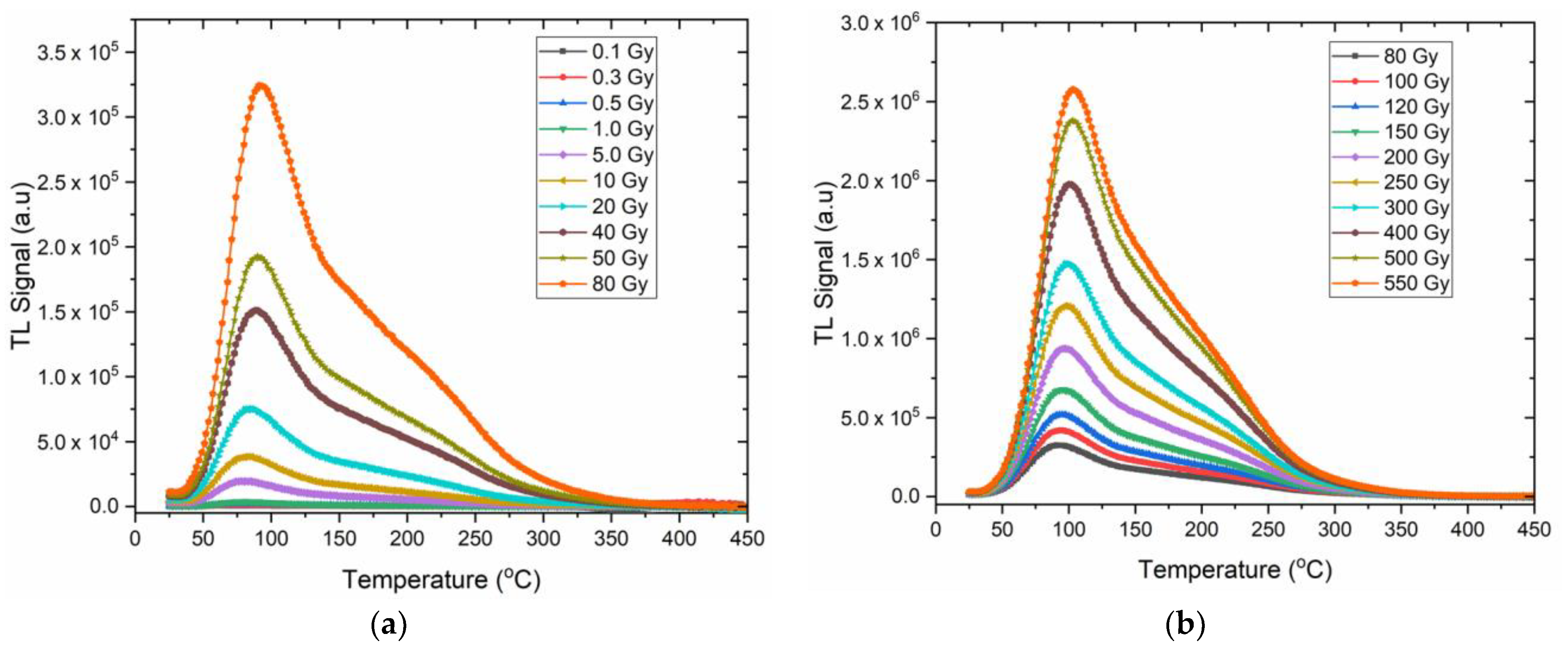
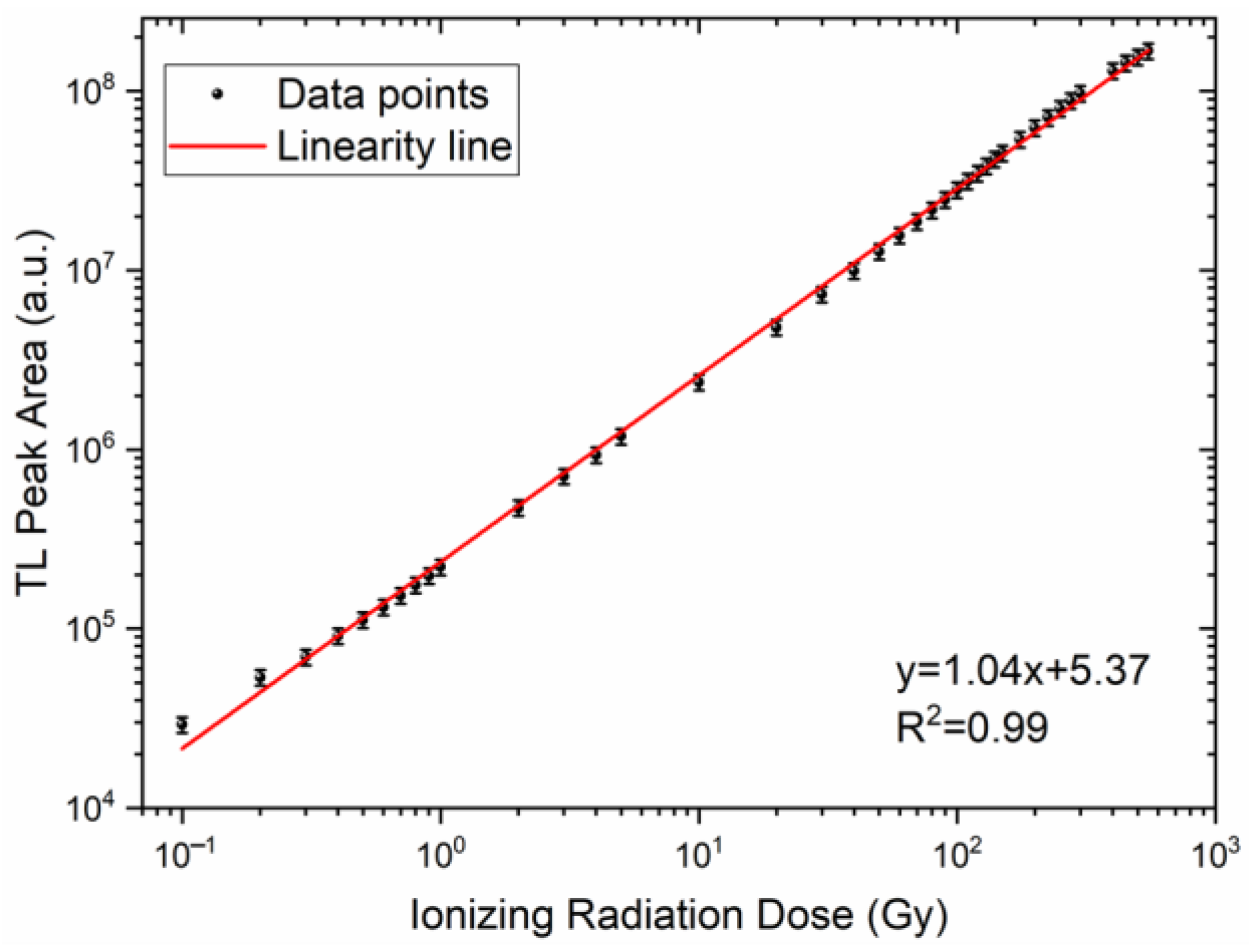
Scanning electron microscope (SEM) images of plagioclase samples taken using 1.00 and 80.00 KX magnification ratios, the Energy Dispersive X-ray Spectroscopy (EDS) analysis spectrum, and the results of the quantitative elemental analysis obtained as a result of the EDS analysis are given in in Figure 1.

As can be seen in Figure 1, when the SEM images, EDS spectra, and elemental composition results are examined, the spectra of potassium (K) in addition to sodium (Na), aluminum (Al), silicon (Si), and oxygen (O) belonging to plagioclase are observed in certain energy regions of the samples. As expected, this indicates the presence of plagioclase and K-feldspar in igneous rocks containing more silica. The reason for the spectrum of the carbon (C) element seen in the EDS results is due to the carbon tape on which the analyzed samples were glued.

3.2. Dose Response

Luminescent materials, particularly insulators and semiconductors, play a crucial role in different dosimetric and spectroscopic applications. Thermoluminescence (TL) is a key parameter for evaluating the dose responses of both natural and synthetic materials to ionizing radiation [1,3]. The dose response refers to the relationship between the absorbed radiation dose and the intensity of the TL signal emitted when the material is heated [1]. However, some materials exhibit supralinearity or saturation at higher doses due to the limitations of trap filling and recombination mechanisms within their crystal structure [2]. The TL method provides insights into the kinetics of trapping and recombination processes, enabling the optimization of materials for specific applications [3,4]. In summary, understanding the dose response of luminescent materials is a cornerstone of TL research. The response of the material to the ionizing radiation doses determines its place in a wide range of applications.

In this study, dose–response experiments, which are essential for research using the TL method, were performed on the plagioclase mineral over a wide dose range (from 0.1 Gy to 550 Gy). A number of selected TL glow curves obtained from the dose–response experiments are shown in Figure 2.

Figure 2 illustrates the TL glow curves of the plagioclase mineral plotted as a function of temperature for various radiation dose values. As can be seen in Figure 2, there is no observed change in the shape of the TL glow curves with increasing dose. In addition, it is observed that both the areas under the glow curves and the peak heights (TL signals) increase with increasing dose. This increase in TL intensity with increasing dose is a well-documented phenomenon in the literature and is primarily attributed to the higher density of charge carriers trapped in luminescence centers (electron traps) as the dose increases. This relationship has been extensively studied and is often described as linear within a certain dose range, followed by potential supralinearity or saturation at higher doses due to limitations in trap filling or recombination dynamics [1,2]. Studies have shown that materials such as plagioclase and LiF:Mg,Ti exhibit a predictable increase in the TL signal under low-to-moderate doses, making them suitable for dosimetric applications [3,4]. The proportional increase in TL intensities with dose is often linked to the growing number of excited electrons captured in the traps, which release their energy as luminescence during heating [2,27].

The areas under the TL radiation curves are plotted as a function of each ionizing radiation dose on a log-log scale, as shown in Figure 3. For each dose value, a data point represents the mean value of the TL measurements obtained from five identical rimmed discs, and the error bars represent the standard deviation.

As can be seen in the graph of peak areas versus radiation dose shown in Figure 3, it can be said that there is a very good linear response between total TL intensity and radiation doses in the dose range of 0.3 Gy to 550 Gy. No radiation damage was observed on the material within the measured dose ranges, nor were any supralinear, sublinear, or saturation dose–response regions detected.

3.3. Glow Curve Analysis

The experimental TL glow curve obtained from the plagioclase samples irradiated with a dose of 50 Gy is shown in Figure 4 with a black square symbol. It can be stated that this experimental glow curve consists of two visible luminescence peaks: a sharp peak around 90 °C and a shoulder-shaped peak around 200 °C. Although the TL glow curve appears to consist of two distinct peaks, a more detailed analysis of the glow curve is necessary. Therefore, the TL glow curve was deconvoluted using the CGCD method with the TLanal program.

Figure 4 shows the TL glow curve of the plagioclase sample irradiated with 50 Gy of beta radiation along with the deconvoluted TL peaks obtained using the CGCD method with the TLanal (v1.0.3) program.

Table 2. TL kinetic parameters of the deconvoluted TL glow curve obtained by the CGCD method for the plagioclase mineral irradiated at a 50 Gy dose.

Peaks	TM (°C)	E (eV)	s (s−1)	b	FOM (%)	Deviation
P1	83	0.842	3.08 × 1012
P2	112	0.848	2.23 × 1014
P3	163	0.852	8.08 × 1013	1.5	0.867	0.016
P4	216	0.857	2.15 × 1012
P5	277	0.890	1.65 × 1012

also shows the parameters of the deconvoluted glow peaks, the figure of merit (FOM), and deviation values for each peak individually.

The quality of deconvolving the TL glow curve into its basic glow peaks is determined by the FOM value, and the expression used to calculate this value where Y_i is the input value and F_i is the best fit value of the TL intensity at temperature T_i is provided below [28]:

$$FOM\left(\%\right)={\displaystyle \frac{\sum _i\left|Y_i-F_i\right|}{\sum _i{Y}_i}}x100$$

(1)

A lower FOM indicates a better quality of fitting, with the ideal FOM being 0, achieved only with a perfect fit. However, FOM values below 1% are generally considered acceptable, taking into account various experimental and theoretical errors in the glow curve measurements and fitting processes [29,30,31]. FOM values exceeding 2% suggest substantial errors in the fitted results.

As seen in Table 2, the FOM value calculated from the deconvolution of the TL glow curve for the samples under investigation is 0.867, indicating that the deconvolution process is of reasonably good quality. Furthermore, the overlap of the experimental and fitted glow curves shown in Figure 4, along with the deviation value of 0.016 calculated for the deconvolution process, indicates that the deconvolution process is of very high quality.

As seen in Figure 4 and Table 2, the TL glow curve obtained from the samples irradiated with a radiation dose of 50 Gy consists of five different glow peaks with general-order kinetics (b = 1.5). The peak temperatures of these glow peaks are located around 83, 112, 163, 216, and 277 °C. The activation energies (or trap depths) calculated for the peaks as a result of the deconvolution are close to each other, ranging between 0.842 eV and 0.890 eV. The frequency factors (attempt to escape factors) corresponding to the electron traps for each glow peak are presented in Table 2, with values ranging from 1.65 × 10¹² s⁻¹ to 2.23 × 10¹⁴ s⁻¹.

3.4. Artificial Neural Network (ANN)

Thermoluminescence (TL) analysis requires precise modelling of dose–response relationships to better understand the behavior of any material exposed to different radiation doses. This study presents the implementation of an artificial neural network (ANN) model to predict the thermoluminescence glow curves of a plagioclase mineral based on the input of different and increasing dose values. The proposed model is implemented by using the neural network toolbox of MATLAB 2024b for data preprocessing, model training, and evaluation.

3.4.1. Dataset

The dataset includes 34 radiation dose values (input values) and corresponding TL glow curves (output values), which are processed and normalized before training. Each of the output values consist of 221 response values. The data were normalized using min–max scaling to improve model convergence and ensure a consistent range of values. The normalized dataset was then split into training, validation, and test sets using stratified partitioning techniques, allocating 70% for training and the remaining 30% for validation and testing. The stratified splitting ensures representative sampling across all dose levels, enhancing the generalization capability of the model.

3.4.2. Performance Evaluation of the ANN Model

The performance of the developed neural network model for predicting TL glow curves was evaluated using three key metrics: Mean Absolute Error (MAE), Mean Squared Error (MSE), and the coefficient of determination ($R^2$).

The MAE, given in Equation (2), measures the average absolute derivation between the predicted (${\widehat{y}}_i$) and actual ($y_i$) values across $n$ observations. By representing the typical deviation in the same unit as the output variable, the MAE offers an intuitive interpretation of the model’s prediction errors.

$$MAE={\displaystyle \frac{1}{n}}\sum \left|y_i-{\widehat{y}}_i\right|$$

(2)

The MSE, given in Equation (3), calculates the average of the squared differences between predicted and actual values. By squaring the errors, the MSE places a stronger emphasis on larger deviations, making it particularly useful for identifying models that may suffer from occasional large errors.

$$MSE={\displaystyle \frac{1}{n}}{\sum \left(y_i-{\widehat{y}}_i\right)}^2$$

(3)

To assess the proportion of variance in the luminescence response explained by the model, the coefficient of determination ($R^2$), shown in Equation (4), was computed, where ${\overline{y}}_i$ represents the mean of the actual observed values. This metric compares the sum of squared residuals to the total sum of squares, where a value closer to 1 indicates a strong correlation between predictions and actual values.

$$R^2=1-{\displaystyle \frac{\sum {(y_i-{\widehat{y}}_i)}^2}{\sum {(y_i-{\overline{y}}_i)}^2}}$$

(4)

The combination of these metrics offers a well-rounded evaluation of the model’s performance, providing information on both the magnitude and distribution of errors. The obtained results demonstrate the model’s effectiveness in accurately predicting TL glow curves based on dose values and demonstrate its potential applicability in thermoluminescence analysis and related fields.

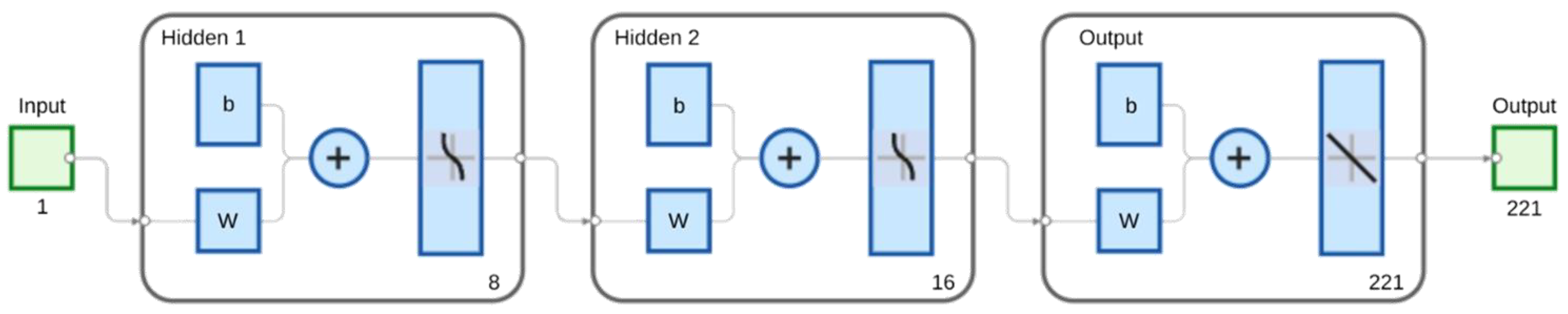
3.4.3. ANN Architecture and Training Parameters

The ANN model is structured with an input layer consisting of a single neuron representing dose values. This is followed by two hidden layers containing 8 and 16 neurons, respectively, designed to capture the complex nonlinear relationships between input and output data. The output layer consists of 221 neurons corresponding to the TL glow curve values (Figure 5).

The model was trained using three different optimization algorithms, LM, BR, and SCG, each offering different advantages in terms of convergence speed, regularization, and computational efficiency. Training was performed for a maximum of 1000 epochs to ensure sufficient learning with a learning rate of 0.001 to control step size during weight updates. A minimum gradient threshold of 10⁻⁷ was set as a stopping criterion to avoid over computation. Furthermore, the training process includes an early stopping mechanism that allows a maximum of 15 validation errors before stopping to avoid overfitting and improve the generalization ability of the model. The critical training parameters of the ANN model configuration are presented in

Table 3. The ANN model training parameters for the plagioclase mineral.

Parameter	Value	Description
Input Layer	1 neuron	Represents the dose values
Hidden Layers	2 hidden layers [8,16] neurons	Number of neurons in the two hidden layers
Output Layer	221 neurons	TL glow curves
Training Algorithm	LM, BR, and SCG	Optimization algorithms
Epochs	1000	Maximum number of training iterations
Learning Rate	0.001	Step size for weight updates
Minimum Gradient	10−7	Stopping criteria to avoid overcomputation
Max Fail	15	Early stopping mechanism

.

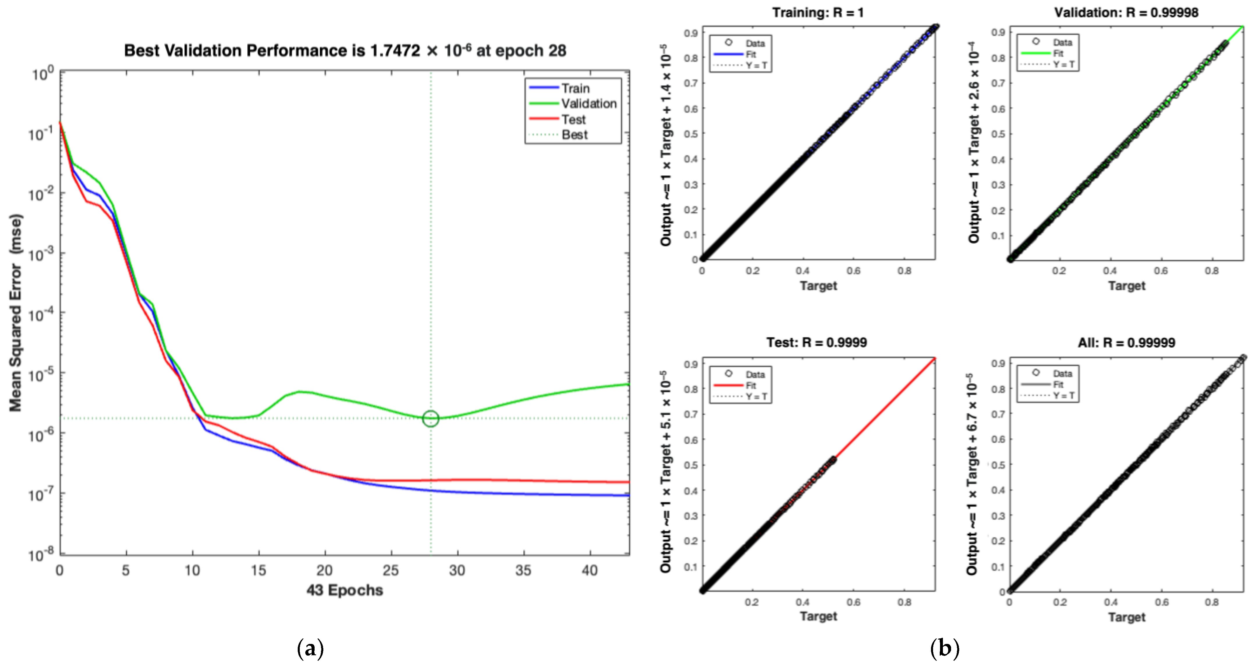
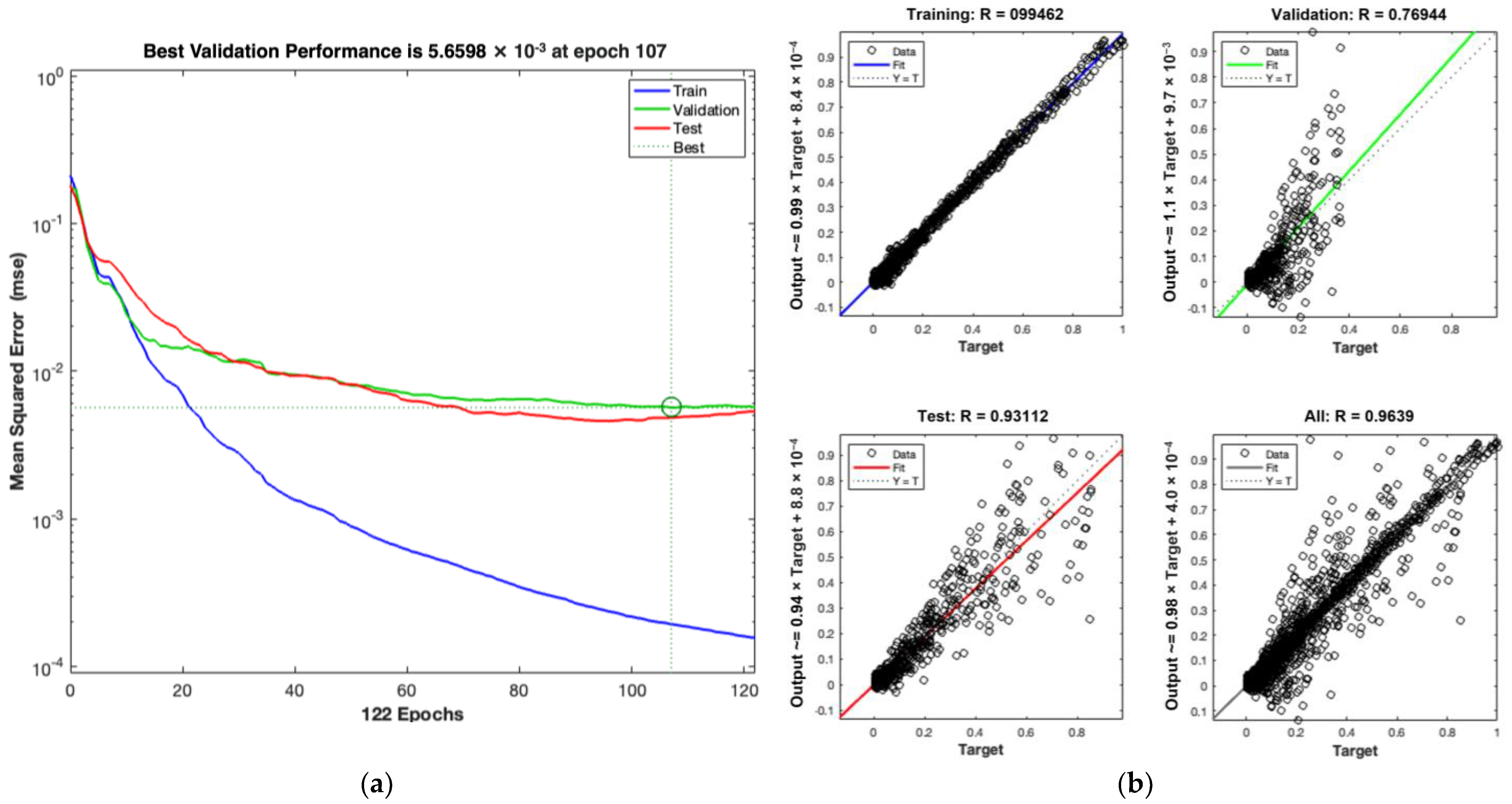
3.4.4. Training Results and Visualization

The comparative analysis of the three optimization algorithms (LM, BR, and SCG) reveals distinct characteristics in terms of convergence speed, generalization ability, and computational efficiency. The simulation performance and regression results of the LM optimization algorithm are presented in Figure 6.

The LM algorithm, known for its fast convergence and suitability for small-to-medium-sized datasets, demonstrated rapid error reduction and reasonably good fitting capabilities. However, it showed a tendency to overfit the data slightly, as indicated by a remarkable gap between the training and test losses, suggesting sensitivity to complex data patterns (Figure 6a).

As shown in Figure 6b, the LM algorithm exhibits a strong correlation between predicted and actual values, with most data points closely aligning with the ideal regression line. The high regression values demonstrate that the model effectively captures the underlying relationships within the data. However, slight deviations observed at higher response values indicate potential overfitting, which could impact the model’s generalization to new data.

The simulation performance and regression results of the BR optimization algorithm are presented in Figure 7.

The BR optimization provided the most balanced performance by effectively minimizing overfitting while maintaining good prediction accuracy (Figure 7a). The training and validation loss curves for BR were closely aligned throughout the training process, confirming its good generalization ability even with limited data.

As shown in Figure 7b, the regression analysis for BR showed the highest correlation between predicted and actual values, achieving the best performance compared to other methods. The predicted data points tightly cluster around the ideal fit line across the entire range of responses. The regularization incorporated within the BR algorithm effectively prevents overfitting and results in a balanced trade-off between bias and variance.

The simulation performance and regression results of the SCG optimization algorithm are presented in Figure 8.

The SCG algorithm, designed for large-scale datasets with memory efficiency, exhibited slower but steady convergence, with a smooth and gradual decrease in loss values (Figure 8a).

The regression performance of the SCG algorithm, as shown in Figure 8b, presents a slightly lower regression (R) value compared to LM and BR, with more noticeable deviations from the ideal line. This proposes that SCG may have a tendency to underfit the data, potentially due to its reliance on a gradient-based optimization process that converges more slowly.

The MSE values indicate that the LM algorithm achieved the lowest error followed by BR and SCG with the highest error, as given in

Table 4. The performance results of the different optimization algorithms.

Algorithm	MAE	MSE	R2 Score
LM	8.45 × 10−4	6.00 × 10−6	0.99895
BR	2.34 × 10−3	3.82 × 10−5	0.99915
SCG	1.45 × 10−2	6.78 × 10−4	0.71337

. In terms of the MAE, which measures the average magnitude of errors, the LM algorithm again outperformed the others with the lowest value, but BR followed closely, while SCG demonstrated the highest error. The results propose that LM and BR provide more accurate and stable predictions, whereas SCG performs a lower level of precision.

The BR algorithm achieved the highest R² value (0.99915), indicating the best predictive performance among these algorithms. LM followed closely with an R² value of 0.99895, showing similar effectiveness. However, SCG, with an R² of 0.71337, exhibited the weakest correlation between the predicted and actual values, suggesting a limited ability to capture the underlying relationships within the data.

In summary, the LM and BR algorithms show the highest performance, with LM showing the lowest prediction errors and BR providing the best generalization. SCG, while computationally efficient, lags in accuracy and precision, making it less suitable for high-accuracy TL glow curve modelling. Although the R² values for the BR and LM algorithms are very high (≥0.998), overfitting was mitigated using stopping criteria, early stopping, regularization (particularly with BR), and stratified data partitioning. The BR algorithm especially demonstrated a well-balanced generalization performance, as validated by the close alignment of training and validation loss curves.

The performance results of the optimization algorithms shown in Table 4 provide valuable information about their predictive capabilities and efficiency in luminescence glow curve modelling.

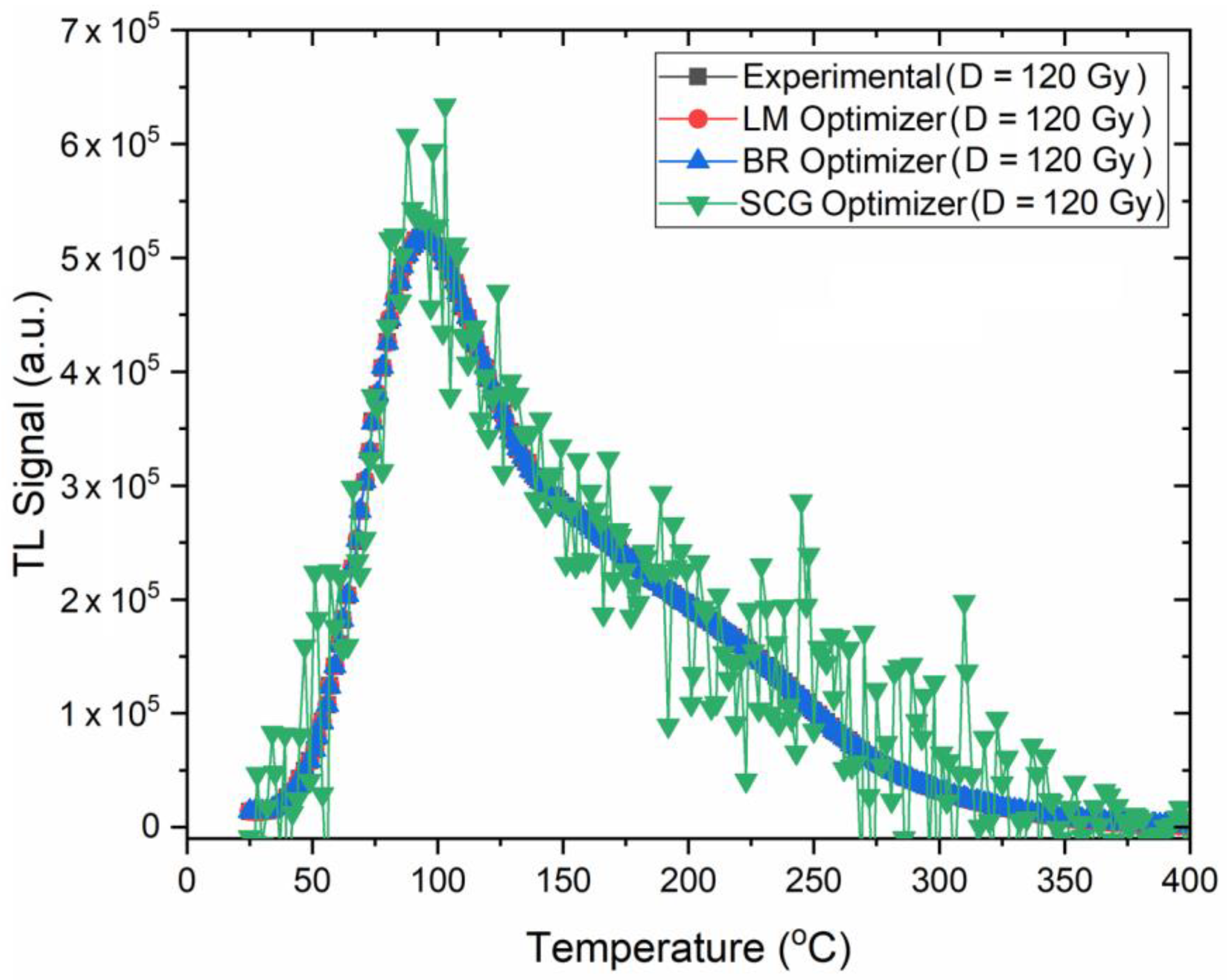
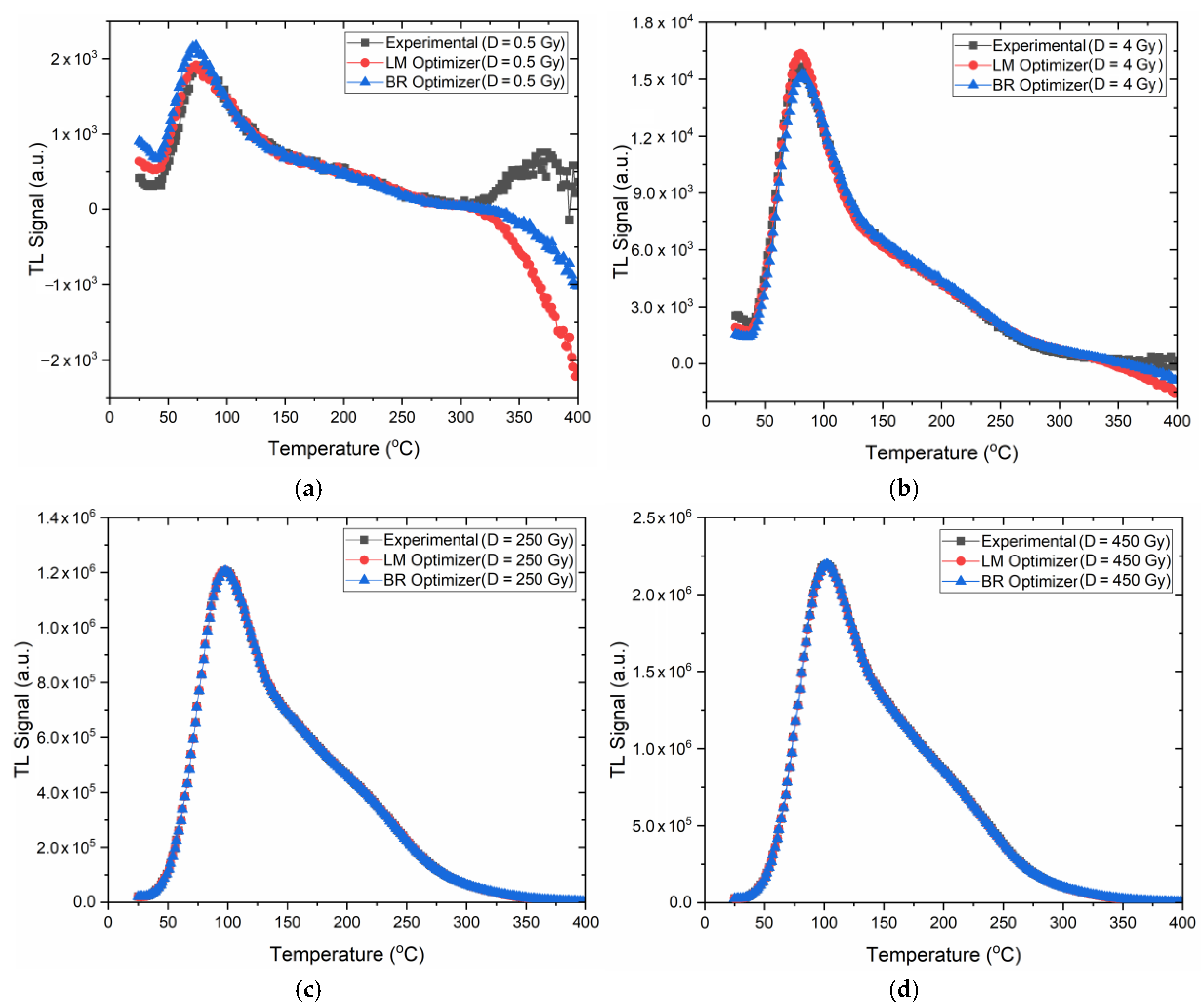
3.4.5. Comparison of Experimental Data with ANN Predicted Data

In this section of the study, the results of the comparison of the experimentally obtained TL glow curves at radiation doses of 0.5, 4, 120, 250, and 450 Gy, which were not used in the training with ANN, and the TL glow curves produced by the ANN model are presented.

The TL glow curve obtained experimentally as a result of the irradiation of the plagioclase mineral with a radiation dose of 120 Gy and the glow curves produced by the LM, BR, and SCG optimizers in the ANN model are shown in Figure 9.

As can be seen in Figure 9, the glow curves obtained from the LM and BR optimizers overlap with the experimental glow curve, while the glow curve obtained from the SCG optimizer shows deviations. Therefore, in the following comparisons, only the data generated by the LM and BR optimizer are compared with the experimental data. While making these comparisons, graphs obtained at low, medium, and high radiation doses were used to observe the effects of different levels of doses.

The TL glow curves obtained with different radiation doses (0.5, 4, 250, and 450 Gy) experimentally and produced by the LM and BR optimizers are shown in Figure 10.

When all the graphs in Figure 10 are examined, it can be said that both the LM and BR optimizers are able to predict the TL glow curves in accordance with the experimental data.

As can be seen in Figure 10a,b, the experimental TL glow curves at low dose values are not consistent in both low- and high-temperature regions. In many studies, it has been shown that quantum emission in the visible region by the heating unit of the thermoluminescence reader causes a spurious TL signal at low radiation dose levels [32,33,34]. Apart from these spurious signals, room temperature, noise, and background radiation can also affect the data obtained at low dose levels.

Therefore, these experimental deviations at low radiation doses in both low- and high-temperature regions should be considered normal. Due to these deviations, it can be seen in Figure 10a,b that there are some deviations in the TL glow curve predictions made with the LM and BR optimizers at low dose values, both in the low-temperature (<50 °C) and high-temperature (>325 °C) regions. It is also seen in Figure 10c,d that these deviations disappear towards high dose values and the TL glow curve predictions give more qualitative results.

4. Conclusions

In this research, the TL properties of the plagioclase mineral and the prediction of TL glow curves at different ionizing radiation doses with an ANN were studied, and the following results were obtained:

• When the TL response of the mineral to ionizing radiation was evaluated, it was revealed that it showed a linear dose response in the dose range of 0.3 to 550 Gy.
• The TL glow curve of the mineral consists of five different TL glow peaks—in other words, TL glow peaks corresponding to five different electron traps—in accordance with general order kinetics.
• These glow peaks forming the TL glow curve have activation energies (trap depth) of 0.842, 0.848, 0.852, 0.852, 0.857, and 0.890 eV corresponding to temperatures of 83, 112, 163, 216, and 277 °C, respectively.
• Among the optimization algorithms tested, it can be said that the BR algorithm is the most suitable optimization algorithm that can be used in the prediction of TL glow curves obtained at different radiation doses of plagioclase mineral.
• Although the LM algorithm is advantageous in terms of fast convergence and high precision on small datasets, its tendency toward overfitting requires additional refinement techniques.
• Although SCG is computationally efficient, it requires longer training times and larger training sets to achieve optimum accuracy.
• Unlike LM and SCG, BR emerged as the most appropriate choice in this study by establishing a good balance between bias and variance and was able to produce reliable results in wide dose ranges thanks to its high generalization performance.

Although BR emerged as the most appropriate algorithm approach in this study, future studies can use approaches such as hybrid and deep learning algorithms that combine the strengths of these three algorithms to further improve model performance on different datasets.

The ANN can be trained on experimental radiation curve data to predict unknown doses, correct for fading effects, or reconstruct irradiation timing, as demonstrated in recent studies [12,15] using both simulated and real-world datasets. Furthermore, the ANN architectures such as feed forward or shallow networks can accurately predict fade time and irradiation dose simultaneously, outperforming conventional deconvolution techniques in terms of robustness and computational time. Furthermore, in mineral characterization studies where TL signals are affected by complex defect distributions or anisotropic crystal structures (as seen in plagioclase feldspars), the flexibility of ANNs allows them to learn from data patterns without assuming specific physical models. This becomes particularly valuable when investigating variables such as trap distributions, compositional variations, or irradiation environments. Finally, as the volume of luminescence data increases, integrating machine learning (ML) frameworks, including convolutional networks or ensemble learning, with ANN-based regression models enables a method for real-time, automated dose assessment or classification tasks. Therefore, the synergy between luminescence analysis and ANN methodologies offers significant potential for researchers to advance both basic and applied research in the fields of dosimetry, geochronology, and nuclear physics.

References

1. McKeever, S.W.S. Thermoluminescence of Solids; Cambridge University Press: Cambridge, UK, 1985; ISBN 9780521368117. [Google Scholar]
2. Chen, R.; McKeever, S.W.S. Theory of Thermoluminescence and Related Phenomena; World Scientific: Singapore, 1997; ISBN 978-981-02-2295-6. [Google Scholar]
3. Bøtter-Jensen, L.; McKeever, S.W.S.; Wintle, A.G. Optically Stimulated Luminescence Dosimetry; Elsevier: Amsterdam, The Netherlands, 2003; ISBN 978-0444506849. [Google Scholar]
4. Pagonis, V.; Kitis, G.; Furetta, C. Numerical and Practical Exercises in Thermoluminescence. In Numerical and Practical Exercises in Thermoluminescence; Springer: New York, NY, USA, 2006; pp. 1–208. [Google Scholar] [CrossRef]
5. Wazir-ud-Din, M.; ur-Rehman, S.; Mahmood, M.M.; Ahmad, K.; Hayat, S.; Siddique, M.T.; Kakakhel, M.B.; Mirza, S.M. Computerized Glow Curve Deconvolution (CGCD): A Comparison Using Asymptotic vs Rational Approximation in Thermoluminescence Kinetic Models. Appl. Radiat. Isot. 2022, 179, 110014. [Google Scholar] [CrossRef]
6. Yüksel, M.; Dogan, T.; Balci-Yegen, S.; Akca, S.; Portakal, Z.G.; Kucuk, N.; Topaksu, M. Heating Rate Properties and Kinetic Parameters of Thermoluminescence Glow Curves of La-Doped Zinc Borate. Radiat. Phys. Chem. 2018, 151, 149–155. [Google Scholar] [CrossRef]
7. Furetta, C. Handbook of Thermoluminescence; World Scientific: Singapore, 2003; ISBN 978-981-238-240-5. [Google Scholar]
8. Amit, G.; Datz, H. Improvement of Dose Estimation Process Using Artificial Neural Networks. Radiat. Prot. Dosim. 2019, 184, 36–43. [Google Scholar] [CrossRef] [PubMed]
9. Lotfalizadeh, F.; Faghihi, R.; Bahadorzadeh, B.; Sina, S. Unfolding Neutron Spectra from Simulated Response of Thermoluminescence Dosimeters inside a Polyethylene Sphere Using GRNN Neural Network. J. Instrum. 2017, 12, T07007. [Google Scholar] [CrossRef]
10. Isik, E.; Isik, I.; Toktamis, H. Analysis and Estimation of Fading Time from Thermoluminescence Glow Curve by Using Artificial Neural Network. Radiat. Eff. Defects Solids 2021, 176, 765–776. [Google Scholar] [CrossRef]
11. Toktamis, D.; Er, M.B.; Isik, E. Classification of Thermoluminescence Features of the Natural Halite with Machine Learning. Radiat. Eff. Defects Solids 2022, 177, 360–371. [Google Scholar] [CrossRef]
12. Theinert, R.; Kröninger, K.; Lütfring, A.; Mender, S.; Mentzel, F.; Walbersloh, J. Fading Time and Irradiation Dose Estimation from Thermoluminescent Dosemeters Using Glow Curve Deconvolution. Radiat. Meas. 2018, 108, 20–25. [Google Scholar] [CrossRef]
13. Dogan, T. A Comparison of the Use of Artificial Intelligence Methods in the Estimation of Thermoluminescence Glow Curves. Appl. Sci. 2023, 13, 13027. [Google Scholar] [CrossRef]
14. Kitis, G.; Pagonis, V. On the Need for Deconvolution Analysis of Experimental and Simulated Thermoluminescence Glow Curves. Materials 2023, 16, 871. [Google Scholar] [CrossRef]
15. Kröninger, K.; Mentzel, F.; Theinert, R.; Walbersloh, J. A Machine Learning Approach to Glow Curve Analysis. Radiat. Meas. 2019, 125, 34–39. [Google Scholar] [CrossRef]
16. Li, D.; Zhao, H.; Xie, H.; Khormali, F.; Sun, A.; Zhang, S. Influence of Na-Feldspar Grains within the K-Feldspar Fraction on Sediments IRSL Dating. Quat. Int. 2024, 698, 49–58. [Google Scholar] [CrossRef]
17. Larsen, E.; Johannessen, N.E.; Kowalczuk, P.B.; Kleiv, R.A. Selective Flotation of K-Feldspar from Na-Feldspar in Alkaline Environment. Min. Eng 2019, 142, 105928. [Google Scholar] [CrossRef]
18. Aydın, Ş.N. Petrology of Akçataş Granite (Nevşehir) in the Middle Anatolian Massive. Bull. Miner. Res. Explor. 1991, 112, 58. [Google Scholar]
19. Chung, K.S.; Choe, H.S.; Lee, J.I.; Kim, J.L.; Chang, S.Y. A Computer Program for the Deconvolution of Thermoluminescence Glow Curves. Radiat. Prot. Dosim. 2005, 115, 343–349. [Google Scholar] [CrossRef] [PubMed]
20. Chung, K.S.; Choe, H.S.; Lee, J.I.; Kim, J.L. A New Method for the Numerical Analysis of Thermoluminescence Glow Curve. Radiat. Meas. 2007, 42, 731–734. [Google Scholar] [CrossRef]
21. de Jesús Rubio, J. Stability Analysis of the Modified Levenberg–Marquardt Algorithm for the Artificial Neural Network Training. IEEE Trans. Neural Netw. Learn. Syst. 2021, 32, 3510–3524. [Google Scholar] [CrossRef]
22. Makomere, R.; Rutto, H.; Koech, L.; Banza, M. The Use of Artificial Neural Network (ANN) in Dry Flue Gas Desulphurization Modelling: Levenberg–Marquardt (LM) and Bayesian Regularization (BR) Algorithm Comparison. Can. J. Chem. Eng. 2023, 101, 3273–3286. [Google Scholar] [CrossRef]
23. Lek, S.; Park, Y.S. Artificial Neural Networks. In Encyclopedia of Ecology, Five-Volume Set; Elsevier: Amsterdam, The Netherlands, 2008; Volume 1–5, pp. 237–245. [Google Scholar]
24. Foresee, F.D.; Hagan, M.T. Gauss-Newton Approximation to Bayesian Learning. In Proceedings of the International Conference on Neural Networks (ICNN’97), Houston, TX, USA, 9–12 June 1997; IEEE: Houston, TX, USA, 1997; Volume 3, pp. 1930–1935. [Google Scholar]
25. Møller, M.F. A Scaled Conjugate Gradient Algorithm for Fast Supervised Learning. Neural Netw. 1993, 6, 525–533. [Google Scholar] [CrossRef]
26. Babani, L.; Jadhav, S.; Chaudhari, B. Scaled Conjugate Gradient Based Adaptive ANN Control for SVM-DTC Induction Motor Drive. In Proceedings of the Artificial Intelligence Applications and Innovations, Thessaloniki, Greece, 16–18 September 2016; Iliadis, L., Maglogiannis, I., Eds.; Springer International Publishing: Cham, Switzerland, 2016; pp. 384–395. [Google Scholar]
27. Guérin, G. Some Aspects of Phenomenology and Kinetics of High Temperature Thermoluminescence of Plagioclase Feldspars. Radiat. Meas. 2006, 41, 936–941. [Google Scholar] [CrossRef]
28. Balian, H.G.; Eddy, N.W. Figure-of-Merit (FOM), an Improved Criterion over the Normalized Chi-Squared Test for Assessing Goodness-of-Fit of Gamma-Ray Spectral Peaks. Nucl. Instrum. Methods 1977, 145, 389–395. [Google Scholar] [CrossRef]
29. Sunta, C.M.; Ayta, W.E.F.; Chubaci, J.F.D.; Watanabe, S. General Order and Mixed Order Fits of Thermoluminescence Glow Curves—A Comparison. Radiat. Meas. 2002, 35, 47–57. [Google Scholar] [CrossRef]
30. Mandowski, A.; Bos, A.J.J. Explanation of Anomalous Heating Rate Dependence of Thermoluminescence in YPO4:Ce3+, Sm3+ Based on the Semi-Localized Transition (SLT) Model. Radiat. Meas. 2011, 46, 1376–1379. [Google Scholar] [CrossRef]
31. Sature, K.R.; Patil, B.J.; Dahiwale, S.S.; Bhoraskar, V.N.; Dhole, S.D. Development of Computer Code for Deconvolution of Thermoluminescence Glow Curve and DFT Simulation. J. Lumin. 2017, 192, 486–495. [Google Scholar] [CrossRef]
32. Burch, W.M. Thermoluminescence, Low Radiation Dosage and Black-Body Radiation. Phys. Med. Biol. 1967, 12, 523. [Google Scholar] [CrossRef]
33. Liu, F.; Liang, Y.; Chen, Y.; Pan, Z. Divalent Nickel-Activated Gallate-Based Persistent Phosphors in the Short-Wave Infrared. Adv. Opt. Mater. 2016, 4, 562–566. [Google Scholar] [CrossRef]
34. Sakr, E.; Bermel, P. Angle-Selective Reflective Filters for Exclusion of Background Thermal Emission. Phys. Rev. Appl. 2017, 7, 44020. [Google Scholar] [CrossRef]
Figure 1. SEM/EDS analysis results for the plagioclase mineral.
Applsci 15 04260 g001
Figure 2. TL glow curves of plagioclase mineral at (a) 0.1–80 Gy and (b) 80–550 Gy beta radiation dose ranges.
Applsci 15 04260 g002
Figure 3. Response of the TL peak area for the plagioclase to the dose of ionizing radiation.
Applsci 15 04260 g003
Figure 4. Deconvoluted TL glow curve of the plagioclase irradiated with 50 Gy of beta radiation.
Applsci 15 04260 g004
Figure 5. Architecture of the proposed ANN model.
Applsci 15 04260 g005
Figure 6. ANN simulation results for LM algorithm: (a) performance validation; (b) the linear regression analysis for the target and output.
Applsci 15 04260 g006
Figure 7. ANN simulation results for the BR algorithm: (a) performance validation; (b) the linear regression analysis for the target and output.
Applsci 15 04260 g007
Figure 8. ANN simulation results for the SCG algorithm: (a) performance validation; (b) the linear regression analysis for the target and output.
Applsci 15 04260 g008
Figure 9. TL glow curves obtained experimentally and with different optimizers (radiation dose, D = 120 Gy).
Applsci 15 04260 g009
Figure 10. TL glow curves obtained from experimental, LM, and BR optimizers for (a) 0.5 Gy, (b) 4 Gy, (c) 250 Gy, and (d) 450 Gy radiation doses.
Applsci 15 04260 g010