Surrogate-Assisted Multi-Objective Optimization of Interior Permanent Magnet Synchronous Motors with a Limited Sample Size

Abstract

Interior permanent magnet synchronous motors (IPMSMs) are critical for electric vehicle traction and industrial systems, yet optimizing their performance under high-dimensional design spaces remains computationally challenging. This study proposes a surrogate-assisted multi-objective optimization framework tailored for limited sample sizes. The methodology integrates random forest (RF) and analysis of variance (ANOVA) for variable importance analysis to reduce model complexity, followed by a Generalized Regression Neural Network (GRNN) to establish an efficient surrogate model. A multi-objective particle swarm optimization (MOPSO) algorithm generates Pareto-optimal solutions, while an entropy-weighted distance metric objectively selects the final design. Experimental results demonstrate that the optimized IPMSM achieves a 4.62% increase in average output torque, a 0.15% improvement in efficiency, and a 10.48% reduction in torque ripple compared to the prototype. Finite element analysis validates the consistency between predicted and simulated outcomes, with relative errors below 2.92%. The framework effectively balances computational efficiency and accuracy, offering a data-driven approach for motor optimization under constrained experimental resources.

1. Introduction

Interior permanent magnet synchronous motors (IPMSMs) are widely used in electric vehicle (EV) traction and industrial servo systems due to their high power density, high speed range and high efficiency [1]. It is still significant to optimize motor average output torque, efficiency while reducing torque fluctuations in order to enhance motor performance, improve motor energy consumption, suppress motor noise and stabilize output power [2].

Traditional multi-objective optimization of IPMSMs relies on large scale finite elements simulations, but the cost of computation increases significantly for a contradiction between high-dimensional design parameters and limited sample capacity [3]. To reduce computational consumption, the surrogate-assisted multi-objective optimization method has wide applications in the field of multi-objective optimization of motors. Ref. [4] proposed a surrogate-based model optimization process for permanent magnet synchronous motors (PMSMs), which uses a comprehensive criterion for model evaluation and selection that takes into account both prediction accuracy and time consumption, and compares the prediction performance of four algorithms, namely Multi-Layer Perceptron (MLP), Generalized Regression Neural Network (GRNN), Support Vector Regression (SVR) and Kriging. In the arithmetic example, the MLP had a better prediction performance for all optimization objectives. Ref. [5] proposed a data-driven-based multi-objective optimization framework of a PMSM with a limited sample size that uses 200 sample points to train an SVR model. Both root mean square error (RMSE) and $R^2$ score achieved the demand of prediction precision. Ref. [6] proposed a fast multi-objective optimization algorithm for electromagnetic components based on an Adaptive Neural Network (Adaptive NN) that updates the weights during the optimization process, which effectively accelerates the optimization computation time without losing the optimization quality. Ref. [7] compared 11 surrogate models based on RMSE during the process of multi-objective optimization of an EV’s traction motor. Kriging, Gradient Boosting Decision Tree (GBDT), MLP and Radial Basis Function (RBF) methods were chosen for different optimization objectives to build the surrogate model to minimize the RMSE for each objective, and the optimization results predicted by the surrogate model were very close to the validation results of finite elements.

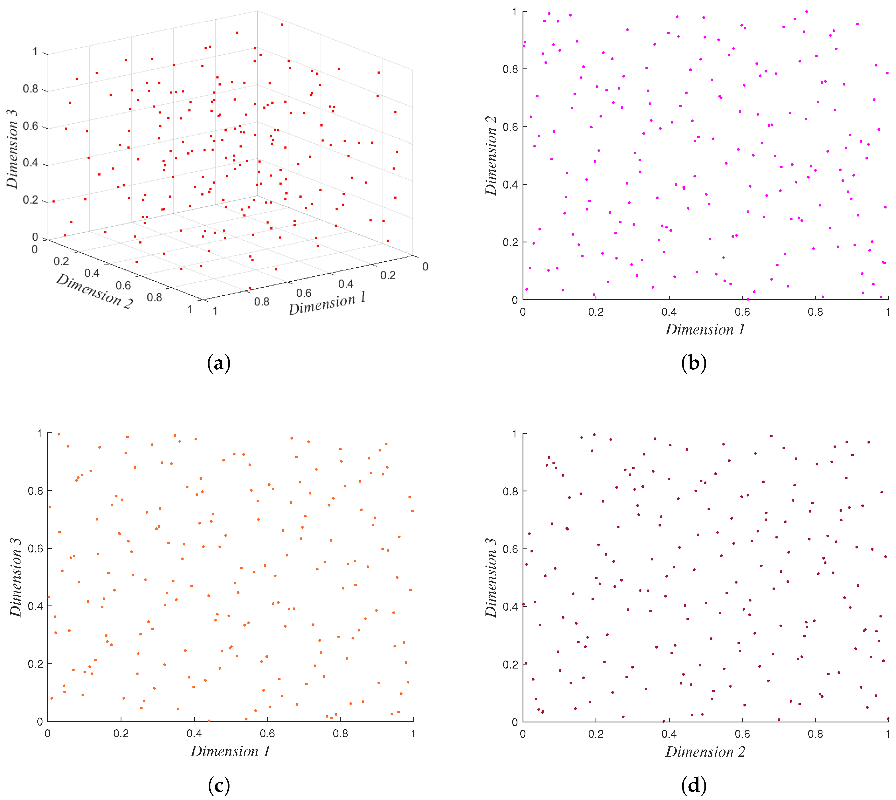
In the process of building surrogate models, a series of experimental design methods are introduced to achieve modeling under finite samples of motors. Under high-dimensional limited samples, the parameters of the model may be biased, thus leading to a decrease in prediction accuracy [8], so it is important to choose a suitable way to fill the experimental space. Among the experimental space-filling designs, Latin hypercube sampling (LHS) is widely used in motor optimization, which seeks to maximize the acquisition of information about the unknown design space while minimizing the number of samples by optimizing the sample point selection strategy [9,10,11,12].

It is obvious that selecting key design parameters that have significant impacts while eliminating unnecessary or redundant parameters could lead to a lower model complexity. There are various approaches to selecting key variables. Here, they are simply grouped into two categories: statistically based analysis methods, which are often described as sensitivity or correlation analysis, and machine learning-based analysis methods, which are usually described as feature selection. 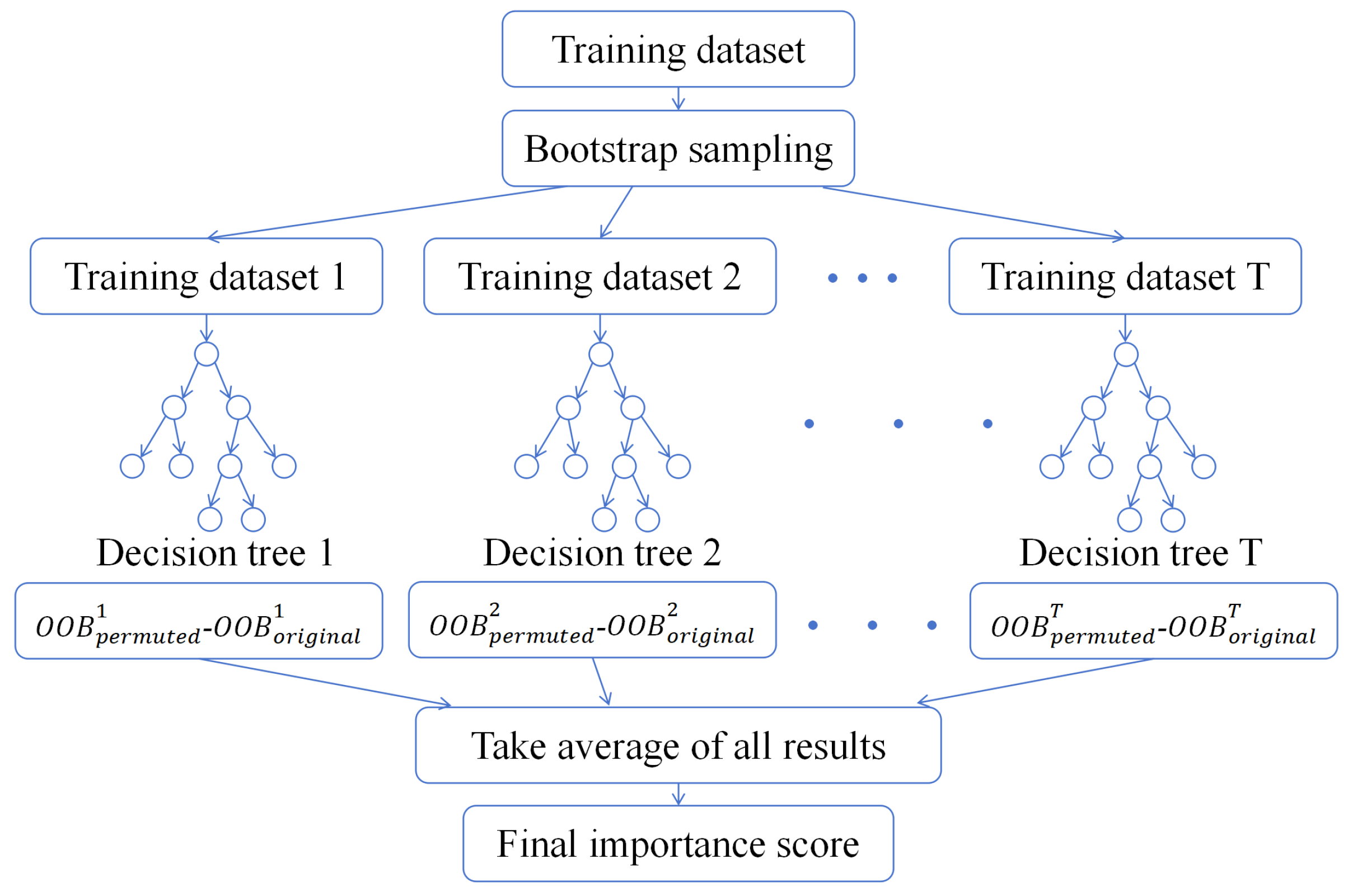Commonly used statistically based analysis methods are Pearson correlation analysis [13,14], Spearman correlation analysis [15], analysis of variance (ANOVA) [5], signal-to-noise ratio analysis [5,16], etc. Among the commonly used machine learning-based analysis methods, random forest (RF)-based feature selection methods stand out in motor optimization. Ref. [17] obtained VI values to represent the relative importance of the design variables based on the errors before and after performing variable substitution during random forest training. Ref. [18] considered the relative importance of the input variables as the default output when calling the random forest algorithm in the Python sklearn package, so it was directly adopted as the basis for selecting the key design variables. The main difference between the two approaches is that the statistically based analysis methods focused only on the significance of the effect of the design variables on the objective variables under statistical significance, while the machine learning-based analysis methods are more inclined to focus on the effect of the design variables on the predictive performance of the model. However, we note that few studies combining the two have been reported.

Factors such as strong coupling between motor parameters and nonlinearity of the objective function cause multi-objective optimization to fall into local optimums and the optimization objectives are difficult to be weighed, so a variety of intelligent optimization algorithms have been introduced to solve the problem [19]. Ref. [20] built a surrogate model with a pyramidal neural network (PNN) and used the Quantum Bat Algorithm (QBA) to optimize IPMSMs, which obtained higher output power and lower loss. Ref. [7] built a surrogate model with the Kringing method and used the Non-dominated Sorting Genetic Algorithm II (NSGA-II) multi-objective optimization algorithm to optimize the efficiency and torque fluctuation of a permanent magnet-assisted synchronous reluctance motor (PMASRM). After optimization, the PMASRM gained higher efficiency and less torque fluctuation. The results were well verified. Swarm intelligent optimization algorithm has stronger robustness, simple structure, less overhead, and self-organization; thus, the multi-objective particle swarm optimization (MOPSO) algorithm is widely used. Based on PSO for the PMSM’s electromagnetic performance of multi-objective optimization, the results of [21] show that the cogging torque has been effectively reduced, the magnitude of the reverse electromotive force has been reduced, the flux density is in a reasonable range, and the electromagnetic performance of the motor has been improved. Ref. [22] used the Taguchi method and PSO to optimize an 8-pole, 48-slot IPMSM’s average output torque, torque fluctuation, and iron loss. The results show that the average output torque is improved, the torque fluctuation and iron loss are suppressed, and the effectiveness of the Taguchi method-PSO hybrid algorithm is verified. Ref. [23] improved the weight coefficients of the PSO algorithm and used it to carry out multi-objective optimization of the Yokeless And Segmented Armature (YASA) motor in order to optimize the average output torque, the torque fluctuation, and the motor output power. The results showed that the motor output power and average output torque are improved, while torque fluctuation is effectively suppressed, and the effectiveness of the optimization was proven through experiments. Ref. [24] used the PSO based on adaptive inertia weights to carry out multi-objective optimization of the rotor pole–parallel hybrid excitation synchronous marine motors, which results in the improvement of the motor’s torque, suppression of torque fluctuation and optimization of the no-load electromotive force.

The multi-objective optimization algorithm gives a series of Pareto non-dominant solutions in which the final optimization result will be selected. For the selection of the Pareto optimal solution, practical feasibility and cost-effectiveness need to be considered, and the selection in engineering often relies on practical experience and skills [25], which is somewhat subjective. However, the objective selection method of Pareto’s optimal solution has also gained attention. In ref. [26], a Pareto optimal solution ranking approach based on the R-method is proposed. The Technique for Order Preference by Similarity to Ideal Solution (TOPSIS) method was used in the study [27] to select the Pareto optimal solution by measuring the distance between the solution and the optimal worst-case point. The gray relation analysis (GRA) was used as a basis for ranking the Pareto solution set in ref. [28]. Selection methods based on information entropy have received much attention. The information entropy (Shannon entropy) was firstly proposed by C.E. Shannon in [29]. On this basis, various types of algorithms based on Shannon entropy have gained wide extension and application. Ref. [30] proposed a differential entropy-based compactness index to measure compactness in scenarios such as transportation systems. Based on a large amount of data and theoretical analysis, ref. [31] analyzes the effect of entropy weight on TOPSIS and proposes an entropy-based TOPSIS with adjustable weight coefficients.

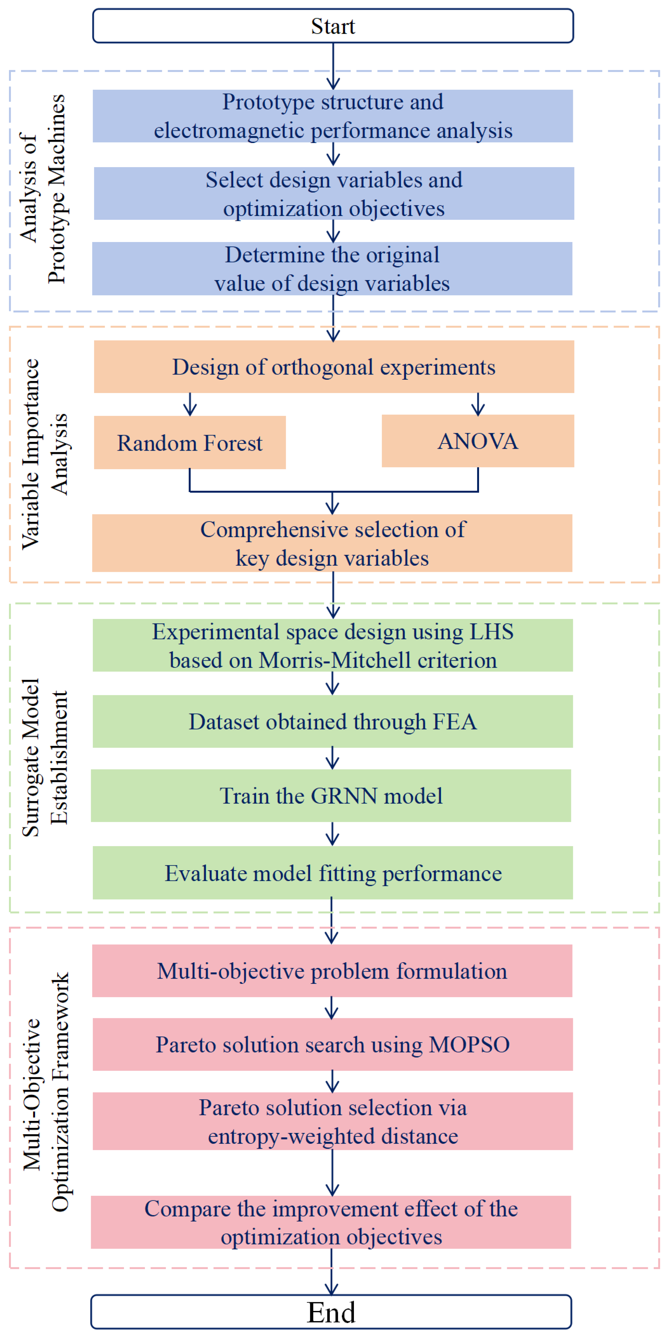
This article proposes a surrogate assisted multi-objective optimization framework with limited sample size, and the core work includes the following:

• Variable importance analysis using RF + ANOVA, which focuses on both the contribution of design variables on model prediction and the sensitivity of each design variable on optimization objectives, has combined machine learning and statistical methods. Variables selected in this way possess both model predictive utility and high sensitivity.
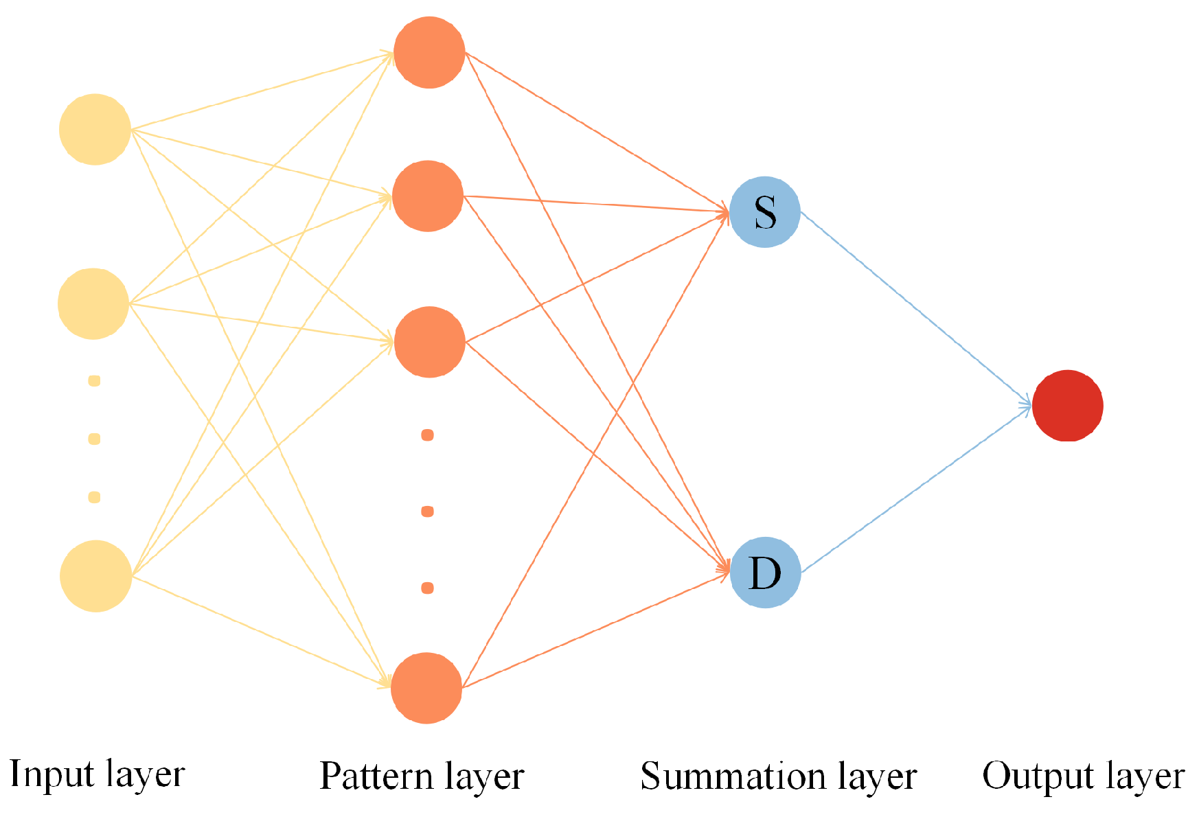
• A surrogate model is established using a GRNN with excellent results under limited samples, whose mathematical foundation has a fixed architecture and is controlled by a single hyperparameter, simplifying parameter adjustment.
• An objective selection method of Pareto’s optimal solution based on “entropy weight distance” is proposed, which distinguishes the weights of different performance indexes and avoids the dependence on experts’ experience in the selection.

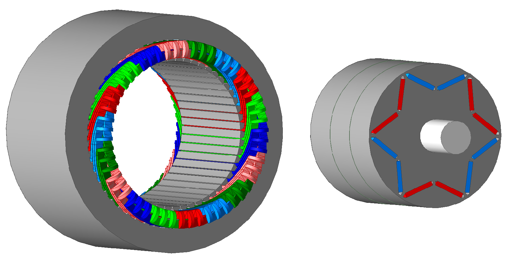
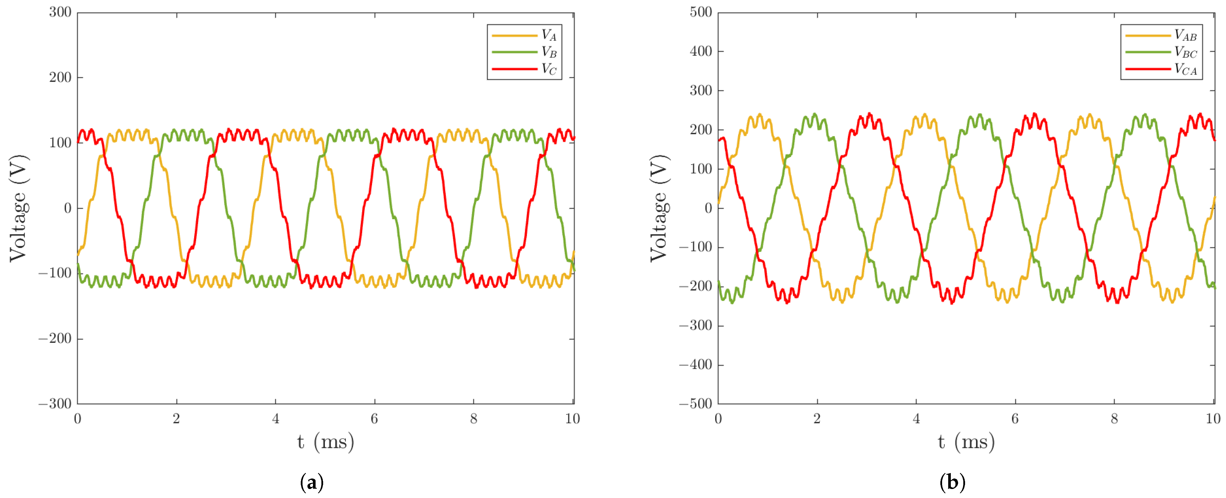
In this paper, Section 2 describes the structure, electromagnetic performance, design variables and optimization variables of the IPMSM prototype; Section 3 carries out the importance analysis of each design variable; Section 4 describes the multi-objective optimization problem and constructs the surrogate model by a GRNN; Section 5 obtains the Pareto frontier through the MOPSO algorithm, and selects the Pareto optimal solution by the “entropy weight distance” method to select the Pareto optimal solution; and Section 6 concludes this article. The flowchart of this study is delineated in Figure 1.

2. Analysis of Prototype Machines

2.1. Prototype Machines Structure

This study focuses on a 100 kW IPMSM designed for EV applications. The prototype motor design adopts a 6-pole 54-slot double-layer short-pitch-distributed winding with a coil pitch of 8 to suppress harmonic component while maintaining a relatively high electromotive force (EMF) amplitude. The rotor is featured with a V-shaped interior permanent magnet to concentrate the magnetic field. The main parameters of the prototype machine is shown in

Table 1. Main parameters of prototype IPMSM.

Parameter	Values
Rated power	100 kW
Rated speed	6000 rpm
Max speed	12,000 rpm
Material of stator core	DW315 Silicon steel sheet
Material of rotor core	DW315 Silicon steel sheet
Material of conductor wire	Copper
Material of PMs	NdFeB N35
Outer diameter of stator	250 mm
Inner diameter of stator	153 mm
Axial length	150 mm
Slot tooth width	5 mm

. The 3D model of the motor is shown schematically in Figure 2.

2.2. Analysis of Electromagnetic Performance

The analysis of the prototype machine is performed by a finite element model (FEM), which is shown in Figure 3a. The mesh arrangement is shown in Figure 3b. The materials in each part of the IPMSM are assigned according to the corresponding entries in Table 1. One section mesh is applied to the solid parts of the IPMSM to better analyze the high-frequency electromagnetic field while the “band region”, which covers the whole rotating area including rotor and air gap, has an in-section mesh to meet the basic requirements of finite element analysis. Due to the need for a special consideration of high-frequency eddy current losses, additional fine mesh is applied to the permanent magnets. The total number of elements eventually reaches 7214.

The simulation operating point was selected at the rated speed of 6000 rpm. Under no load, the phase EMF and line EMF waveforms are shown in Figure 4. For the defined loading condition, a 300 A RMS sinusoidal phase current with a 16° current advance angle was implemented as the representative operational scenario. The balanced three-phase excitation with frequency-synchronized 120° phase spacing was applied, resulting in an output torque as depicted in Figure 5a, and the line EMF waveform is shown in Figure 5b. The output power reached approximately 100 kW, and the system efficiency was calculated as 98.05%. (This value is high due to the fact that this finite element analysis only considers iron losses and permanent magnet eddy current losses and does not take into account mechanical losses which are more difficult to quantify.) All finite element results presented hereafter were obtained under this characterized load configuration (300 A RMS, 16° current angle).

2.3. Design Variables and Optimization Objectives

Considering the energy consumption and output requirements of electric vehicle traction motors, the optimization objectives were selected as average output torque ($T_{av}$), motor efficiency ($\eta$), and torque ripple ($\Delta T$). Six design variables were initially identified: stator slot depth, air gap length, PM thickness, PM width, flux barrier thickness and V-shaped pole base radius. These variables are annotated in Figure 6, with their symbolic representations and initial values detailed in

Table 2. Design parameters of the IPMSM.

Parameter	Symbol	Original Value
Air gap length	${\delta }_g$	0.6 mm
Flux barrier thickness	$b_r$	3 mm
PM thickness	$b_m$	4 mm
Slot height	$h_s$	20 mm
PM width	$l_m$	50 mm
V-shaped pole base radius	$R_m$	37.5 mm

.

3. Variable Importance Analysis

The objective of variable importance analysis is to systematically identify influential design variables that critically affect motor performance by eliminating redundant or non-significant variables. This process reduces model complexity, mitigates the risk of overfitting, and improves computational efficiency for subsequent optimization tasks.

To comprehensively identify key design variables, we implemented a dual-strategy methodology: RF and ANOVA. RF focuses on the contribution of design variables to the model’s predictions, while analysis of variance examines the sensitivity of design variables to optimization objectives. Variables consistently prioritized through both approaches were retained for subsequent optimization, ensuring the final selection possesses both predictive utility and high sensitivity.

3.1. Experimental Design with Orthogonal Arrays

To create efficient and representative test plans with minimal experiments for subsequent analysis, we adopted the orthogonal experiment design [32]. Considering the rationality of various electromagnetic structural parameters and other aspects of motor performance, we have determined a relatively reasonable variable range. We evenly selected seven levels for each variable within this determined range and then constructed an $L_{49}\left(7^6\right)$ orthogonal table. The six factors and their corresponding levels are outlined in

Table 3. Six experimental factors and their levels.

Factor	Unit	Level 1	Level 2	Level 3	Level 4	Level 5	Level 6	Level 7
${\delta }_g$	mm	0.30	0.50	0.70	0.90	1.10	1.30	1.50
$b_r$	mm	3.00	3.33	3.67	4.00	4.33	4.67	5.00
$b_m$	mm	3.00	3.40	3.80	4.20	4.60	5.00	5.40
$h_s$	mm	15.00	16.67	18.33	20.00	21.67	23.33	25.00
$l_m$	mm	30.00	35.83	41.67	47.50	53.33	59.17	65.00
$R_m$	mm	37.50	39.17	40.83	42.5	44.17	45.83	47.50

.

3.2. Random Forest-Based Variable Importance Quantification

The variable importance measurement in random forest is illustrated in Figure 7. This study employs the out-of-bag (OOB) error-based approach, which leverages the inherent bootstrap sampling mechanism of the algorithm.

During forest construction, each decision tree is trained on a bootstrap sample from the original dataset. Approximately 37% of instances are naturally excluded from each bootstrap sample, forming the OOB validation set for that particular tree. Variable importance is quantified by systematically perturbing variables in these OOB sets. For a target variable, its values are randomly permuted within the OOB data, and the resulting change in prediction accuracy is recorded. Critical variables will induce significant accuracy degradation (manifested as increased OOB error) when permuted, while non-informative variables will show negligible impact [33].

The formal importance score I for a variable is computed as

$$I={\displaystyle \frac{1}{T}}\sum _{i=1}^T(OO{B}_{permuted}^i-OO{B}_{original}^i)$$

(1)

where T denotes the total number of trees, and $OO{B}_{permuted}^i$ and $OO{B}_{original}^i$ represent the OOB error rates before and after variable permutation for the i-th tree, respectively.

The orthogonal experimental design generated 49 samples through an $L_{49}\left(7^6\right)$ orthogonal array, systematically covering six design variables across seven levels. These 49 instances were fully leveraged for random forest training. In accordance with the algorithm’s bootstrap sampling mechanism, each decision tree was constructed using approximately 63% of the data (31 samples), while the remaining 37% (18 samples) inherently formed the OOB validation set. Leveraging the inherent OOB validation mechanism, the model achieved stabilization with 0.0181, 0.0197 and 0.0181 RMSE values for respective objectives as tree numbers increased (Figure 8a), confirming prediction reliability. This approach eliminates the requirement for explicit data partitioning, ensuring that all experimental data contribute synergistically to both model construction and validation.

The importance of each design variable for $T_{av}$, $\eta$ and $\Delta T$ is shown in Figure 8b–d, respectively. As can be seen from Figure 8b–d, the importance scores of ${\delta }_g$ and $R_m$ are all negative, indicating that ${\delta }_g$ and $R_m$ are not important for $T_{av}$, $\eta$ and $\Delta T$, and therefore are not selected as key variables. The importance scores of $b_r$ are negative for both $T_{av}$ and $\eta$, but the importance score for $\Delta T$ is notably positive, indicating that although it is not important for $T_{av}$ and $\eta$, its effect on $\Delta T$ should not be ignored, so $b_r$ is classified as a key variable. The importance scores of $b_m$ and $l_m$ on $T_{av}$, $\eta$ and $\Delta T$ are all high and positive, indicating that they have a high impact on all optimization objectives and are therefore all classified as key variables. The importance scores of $h_s$ for both $T_{av}$ and $\Delta T$ are negative, and the importance score for $\eta$ is positive but low compared to $b_m$ and $l_m$, indicating that it is not important for $T_{av}$ and $\Delta T$ and does not have a noteworthy effect on $\eta$, and is therefore not classified as a significant variable.

Based on the results of RF, the key variables are selected as $b_r$, $b_m$ and $l_m$.

3.3. Analysis of Variance

To further analyze the impact of each design variable on optimization objectives, an analysis of variance was conducted on the six design variables. The variance contributions of each design variable were quantified using the following equations [5]:

$$\left\{\begin{array}{c}\hfill {\displaystyle \mathrm{SSX}=\sum _{i=1}^n{\left[m_{X_i}\left(Y\right)-m\left(Y\right)\right]}^2,}\hfill \\ \hfill {\displaystyle m_{X_i}\left(Y\right)=\frac{m}{n}\sum _{k=1}^n{Y}_k,}\hfill \\ \hfill {\displaystyle m\left(Y\right)=\frac{1}{n}\sum _{j=1}^n{Y}_j.}\hfill \end{array}\right.$$

(2)

where n is the total number of experiments; m denotes the number of variable levels; X is the variable under investigation; Y is the target value; $m_{Xi}\left(Y\right)$ denotes the average value of Y corresponding to the i-th level of variable X; and $m\left(Y\right)$ is the overall average value of Y across all experiments.

The result of ANOVA is presented in

Table 4. Result of variance analysis.

Factor	Tav		$\mathit{\eta }$		$\mathbf{\Delta }\mathit{T}$
	SSX	Proportion	SSX	Proportion	SSX	Proportion
${\delta }_g$	0.0072	0.0022	0.0009	0.0003	0.0261	0.0111
$b_r$	0.0237	0.0071	0.0112	0.0036	0.3128	0.1327
$b_m$	0.6479	0.1950	0.6968	0.2298	0.3169	0.1344
$h_s$	0.0018	0.0005	0.1453	0.0479	0.0685	0.0291
$l_m$	2.6057	0.7840	2.1116	0.6967	1.5746	0.6678
$R_m$	0.0373	0.0112	0.0652	0.0215	0.0590	0.0250

. It can be seen that the design variables with higher importance in the analysis of Section 3.2 all have a more significant sensitivity in the ANOVA. As a result, $b_r$, $b_m$ and $l_m$ are selected as key parameters to be used in further study, while ${\delta }_g$, $h_s$ and $R_m$ will be set to the initial values shown in Table 2.

4. Surrogate Model Establishment

4.1. Experimental Space Design for Modeling

Effective experimental space design is critical for establishing surrogate models that accurately capture system characteristics, including variable coupling effects and input–output mapping relationships. The primary objective is to strategically distribute limited sampling points to achieve maximum spatial coverage while maintaining balanced projection density across all dimensions.

This study employs LHS optimized by the Morris–Mitchell criterion to generate 200 training samples in a three-dimensional design space [34]. Unlike random sampling, LHS ensures uniform marginal distributions through stratified division, where each dimension is partitioned into equal non-overlapping intervals with exactly one sample per interval. While basic LHS guarantees projection uniformity, its spatial coverage may be suboptimal due to random permutation along each axis, potentially resulting in clustered or unevenly distributed samples.

To address this limitation, we applied the Morris–Mitchell space-filling criterion to optimize the spatial distribution of sample points [35]. For a given design matrix $X\in {\mathbb{R}}^{n\times d}$ containing n samples in d dimensions, the optimality metric ${\varphi }_p$ is defined as

$${\varphi }_p={\left(\sum _{i=1}^m{J}_i·d_i^{-p}\right)}^{1/p}$$

(3)

where $d_i$ represents distinct pairwise Euclidean distances between samples, $J_i$ denotes the number of point pairs separated by distance $d_i$, m is the total number of different distance values, and we set p = 10 to control the metric’s sensitivity to small distances. Minimizing ${\varphi }_p$ promotes uniform spatial distribution by penalizing clustered point arrangements.

The optimized sampling configuration, visualized in Figure 9, demonstrates superior space-filling characteristics. The entire sample set achieves a global minimum inter-sample distance of 0.0985 (in normalized space) while maintaining uniform marginal distributions. Subsequently, finite element simulations conducted in ANSYS Maxwell 2024R1 generated paired input–output datasets to train and validate the surrogate model.

This methodology ensures that the surrogate model’s training set adequately captures the design space topology, thereby facilitating accurate modeling of complex electromagnetic relationships between input parameters and performance objectives.

4.2. Surrogate Modeling Based on Generalized Regression Neural Network

The GRNN, a probabilistic neural network variant, enables rapid prediction without iterative training due to its fixed architecture governed by a single hyperparameter $\sigma$ (spread factor) [4]. Unlike backpropagation-based methods, GRNN eliminates weight optimization, making it computationally efficient for small-to-medium datasets [36]. As illustrated in Figure 10, the GRNN architecture consists of four distinct processing layers: input layer, pattern layer, summation layer, and output layer.

The input layer dimension corresponds to the feature space of training samples. In the pattern layer, each neuron computes the Gaussian-transformed Euclidean distance between the input vector X and the i-th training sample $X_i$:

$$D_i=exp\left(-{\displaystyle \frac{\parallel X-X_i{\parallel }^2}{2{\sigma }^2}}\right)$$

(4)

where $\parallel ·\parallel$ denotes the Euclidean norm.

The summation layer integrates contributions from all pattern neurons through two operations:

• S-summation: Weighted sum of target values:

  $$S=\sum _{i=1}^n{Y}_i{D}_i$$

  (5)
• D-summation: Total activation sum:

  $$D=\sum _{i=1}^n{D}_i$$

  (6)

The network output $Y\left(X\right)$ is derived as a normalized weight average:

$$Y\left(X\right)={\displaystyle \frac{S}{D}}={\displaystyle \frac{{\sum }_{i=1}^n{Y}_{i}exp\left(-\frac{\parallel X-X_i{\parallel }^2}{2{\sigma }^2}\right)}{{\sum }_{i=1}^{n}exp\left(-\frac{\parallel X-X_i{\parallel }^2}{2{\sigma }^2}\right)}}.$$

(7)

The architecture inherently performs kernel regression, with $\sigma$ controlling the smoothness of predictions [37]. The optimal spread factor $\sigma$ was determined through 5-fold cross-validation, with $\sigma$ = 0.16 identified as achieving the best trade-off between flexibility and generalization performance. This value minimizes validation errors while preventing overfitting to specific training samples.

4.3. Model Fitting Performance

To evaluate the predictive performance of the surrogate model, 200 FEA-derived datasets were utilized to train the GRNN after max–min normalization, ensuring all inputs and outputs were scaled within [0, 1]. As summarized in

Table 5. Prediction accuracy metrics of different surrogate models.

Model	Factor	RMSE 1	${\mathit{R}}^2$ Score 2
GRNN	$T_{av}$	0.0456	0.964
	$\eta$	0.0426	0.962
	$\Delta T$	0.0382	0.965
SVR	$T_{av}$	0.0653	0.915
	$\eta$	0.0616	0.908
	$\Delta T$	0.0553	0.906
MLP	$T_{av}$	0.0511	0.948
	$\eta$	0.0573	0.920
	$\Delta T$	0.0671	0.862
Kriging	$T_{av}$	0.0466	0.957
	$\eta$	0.0558	0.925
	$\Delta T$	0.0625	0.880

¹ Root mean square error. ² Coefficient of determination.

, compared to SVR, MLP and Kriging, GRNN demonstrated superior and balanced performance across all optimization objectives under the limited samples, consistently achieving the lowest RMSE values and highest $R^2$ scores. As shown in Figure 11, each subplot presents a scatter plot of predicated versus measured values for a certain optimization objective, with a “$y=x$” reference line indicating perfect agreement. The data points for $T_{av}$, $\eta$ and $\Delta T$ all closely align with the reference line. The high consistency between predicted and measured values across all three objectives demonstrates the strong predictive accuracy of the GRNN-based surrogate model. Cross-validation further confirmed the model’s generalization capability, with minimal deviations observed across the design space. This comprehensive performance highlights the GRNN’s effectiveness in capturing nonlinear electromagnetic relationships while maintaining computational efficiency, making it particularly suitable for surrogate-assisted optimization in resource-constrained scenarios.

5. Multi-Objective Optimization Framework

5.1. Multi-Objective Problem Formulation

The multi-objective framework aims to simultaneously maximize average output torque ($T_{av}$), enhance motor efficiency ($\eta$), and minimize torque ripple ($\Delta T$). The design variables include flux barrier thickness ($b_r$), PM thickness ($b_m$), and PM width ($l_m$), which were identified as highly important parameters through prior variable importance analysis in Section 3.

Let the design variable vector be defined as $x={[b_r,b_m,l_m]}^T$. The relationships between the design variables and optimization objectives, established via GRNN in Section 4, are expressed as $T_{av}=f_1\left(x\right),\eta =f_2\left(x\right),\Delta T=f_3\left(x\right)$.

Consequently, we formulate the multi-objective optimization problem as a vector function mapping the design variables x to performance objectives, seeking Pareto-optimal solutions through simultaneous maximization of $T_{av}$, $\eta$ and minimization of $\Delta T$:

$$\begin{array}{cc}\hfill & max{f}_1\left(x\right),f_2\left(x\right)\hfill \\ \hfill & min{f}_3\left(x\right)\hfill \\ \hfill & \begin{array}{cc}\mathrm{s}.\mathrm{t}.\hfill & 3\le b_r\le 5,\hfill \\ \hfill & 3\le b_m\le 5.4,\hfill \\ \hfill & 30\le l_m\le 65.\hfill \end{array}\hfill \end{array}$$

(8)

5.2. Pareto Solution Search via Multi-Objective Particle Swarm Optimization

To resolve the multi-objective optimization problem in Equation (8), a MOPSO algorithm was adopted. MOPSO is a meta-heuristic algorithm inspired by swarm intelligence, which efficiently explores the Pareto-optimal solution space by balancing global exploration and local exploitation capabilities [38]. Its suitability for handling nonlinear, non-convex, and high-dimensional optimization problems aligns well with the characteristics of motor design optimization under limited data condition [39]. The parameter settings for the particle swarm optimization algorithm employed in this study are detailed in

Table 6. Parameter settings for MOPSO algorithm.

Parameter	Value
Number of iterations terminated	500
Particle swarm size	30
Archive size	238
Number of design variables	3
Particle velocity range	−0.3∼0.3

.

Figure 12 presents the Pareto frontiers derived from MOPSO, illustrating the trade-offs among the three performance objectives: average output torque ($T_{av}$), motor efficiency ($\eta$), and torque ripple ($\Delta T$). Figure 12a depicts the 3D Pareto frontier, where each point represents a non-dominated solution balancing the competing objectives. Figure 12b–d project the 3D frontier onto 2D planes, highlighting pairwise relationships between $T_{av}$-$\eta$, $T_{av}$-$\Delta T$ and $\eta$-$\Delta T$, respectively. To be specific, the Pareto relationship between $T_{av}$ and $\eta$ exhibits a synergistic positive correlation resembling a logarithmic growth. The reduction of torque ripple has a conflicting relationship with the improvement of average output torque and efficiency enhancement. The mitigation in torque ripple inevitably requires a compromise in average output torque and efficiency performance, and this contradiction becomes more pronounced when higher levels of average output torque and efficiency are achieved. Therefore, how to balance these three objectives to achieve comprehensive performance improvement—specifically, the selection of Pareto optimal solutions for these three objectives—remains a critical issue worthy of attention.

5.3. Pareto Solution Selection via Entropy-Weighted Distance

To systematically prioritize high-quality solutions from the Pareto-optimal set, an entropy-weighted distance method was employed. This approach combines objective weighting based on information entropy with geometric distance metrics to quantify solution quality while preserving trade-off characteristics. The procedure consists of four steps:

• Data normalization: The performance values of Pareto solutions for each objective were normalized to unify optimization directions. For maximization objectives ($T_{av}$, $\eta$),

  $$y_{ij}={\displaystyle \frac{x_{ij}-min\left(x_j\right)}{max\left(x_j\right)-min\left(x_j\right)}}$$

  (9)
  For minimization objectives ($\Delta T$),

  $$y_{ij}={\displaystyle \frac{max\left(x_j\right)-x_{ij}}{max\left(x_j\right)-min\left(x_j\right)}}$$

  (10)

  where $x_{ij}$ denotes the original value of the j-th objective for the i-th solution, and $y_{ij}$ represents the normalized value.
• Entropy calculation: The information entropy $E_j$ for each objective was computed to quantify its data variability:

  $$p_{ij}={\displaystyle \frac{y_{ij}}{{\sum }_{i=1}^n{y}_{ij}}}$$

  (11)

  $$E_j=-{\displaystyle \frac{1}{lnn}}\sum _{i=1}^n{p}_{ij}ln{p}_{ij}$$

  (12)

  where n is the number of Pareto solutions, and $p_{ij}$ denotes the proportion of the i-th solution’s contribution to the j-th objective.
• Weight determination: The entropy weight $w_j$ for each objective was derived based on its entropy value:

  $$w_j={\displaystyle \frac{1-E_j}{{\sum }_{k=1}^m(1-E_k)}}$$

  (13)

  where m is the number of objectives [40]. Lower entropy ($E_j$) corresponds to higher weight ($w_j$), reflecting greater decision information contained in the objective [31]. The result of entropy weight for $T_{av}$, $\eta$ and $\Delta T$ is $w_1$ = 0.4010, $w_2$ = 0.2589 and $w_3$ = 0.3404, respectively.
• Entropy-weighted distance evaluation: The composite performance of each Pareto solution was assessed using a weighted Euclidean distance metric:

  $$D_i=\sqrt{w_1{(1-T_{av,i}^{*})}^2+w_2{(1-{\eta }_i^{*})}^2+w_3{(0-\Delta T_i^{*})}^2}$$

  (14)

  where $T_{av,i}^{*}$, ${\eta }_i^{*}$ and $\Delta T_i^{*}$ are values of the objectives in Pareto solutions (normalized to [0, 1]). Solutions with smaller $D_i$ values exhibit balanced performance closer to the ideal point $Y^{*}$ = ${[1,1,0]}^T$ in normalized objective space. Geometrically, this defines an ellipsoid in 3D objective space centered at $Y^{*}$ (Figure 13). The point with the smallest $D_i$ will be chosen as the final Pareto optimal solution.

This methodology enables unbiased selection of optimal designs while retaining critical trade-off information, facilitating informed decision-making in multi-objective optimization scenarios. The final Pareto optimal solution with a minimal $D_i$ of 0.3268 is presented in

Table 7. Result of optimization.

	${\mathit{b}}_{\mathit{r}}$	${\mathit{b}}_{\mathit{m}}$	${\mathit{l}}_{\mathit{m}}$	${\mathit{T}}_{\mathit{av}}$	$\mathit{\eta }$	$\mathbf{\Delta }\mathit{T}$
Prototype	3.00 mm	4.00 mm	50.00 mm	154.96 N·m	98.05%	36.13 N·m
Optimized	4.99 mm	4.96 mm	52.90 mm	162.12 N·m	98.20%	32.35 N·m

after inverse normalization. Corresponding values of design variables are adopted to conduct a FEA validation in which the prediction and simulation values achieve a high degree of consistency (

Table 8. Validation of results.

	${\mathit{T}}_{\mathit{av}}$	$\mathit{\eta }$	$\mathbf{\Delta }\mathit{T}$
Prediction	165.57 N·m	98.24%	33.29 N·m
FEA	162.12 N·m	98.20%	32.35 N·m
Relative Error	+2.13%	+0.04%	+2.92%

). As a result of multi-objective optimization, $T_{av}$ and $\eta$ show increases of 4.62% and 0.15% as $\Delta T$ is suppressed by 10.48%.

5.4. Analysis of Optimization Result

The optimization results demonstrate notable improvements in electromagnetic performance, driven by strategic adjustments to the key design variables ($b_r$, $b_m$ and $l_m$). These variables collectively influence the air gap flux density distribution and thus efficiency and torque characteristics, as detailed below.

The flux barrier thickness $b_r$ increased from 3.00 mm to 4.99 mm. A thicker $b_r$ enhances magnetic isolation between rotor poles, reducing leakage flux and concentrating more magnetic flux in the air gap. This is reflected in the 1.98% increase in the average air gap flux density magnitude (Figure 14a), which directly contributes to the 4.62% improvement in $T_{av}$.

Increasing $b_m$ from 4.00 mm to 4.96 mm strengthens the magnetomotive force (MMF) of the permanent magnets. This elevates the fundamental component of the air gap flux density, which can be seen in Figure 14b, further boosting $T_{av}$. While thicker PMs could elevate eddy current losses (due to larger conductive volume), the $\eta$ gain may primarily stem from reduced iron losses.

The PM width $l_m$ expands from 50.00 mm to 52.90 mm, effectively increasing the effective pole-arc coefficient. This adjustment may improve the spatial distribution of the air gap flux density, reducing harmonic distortion. As shown in Figure 14b, a notable suppression of the 5th, 7th and 17th harmonics can be seen. The total harmonic distortion (THD) of the air gap flux density decreases from 37.67% to 35.37%. This change is likely to reduce iron losses to counter the potential increase in permanent magnet eddy current losses due to increased $b_r$ to maintain $\eta$ at a high level. Smoother flux distribution probably contributes to the 10.48% reduction in $\Delta T$. The expanded $l_m$ also enhances flux linkage, synergizing with $b_r$ and $b_m$ to elevate $T_{av}$.

The above analysis and the validation of finite element simulation (Table 8) prove that the results obtained from the optimization framework proposed in this paper are robust, reasonable and effective.

6. Conclusions

This study presents a surrogate-assisted multi-objective optimization framework for IPMSMs under limited sample constraints, addressing critical challenges in computational efficiency, variable selection, and Pareto solution prioritization.

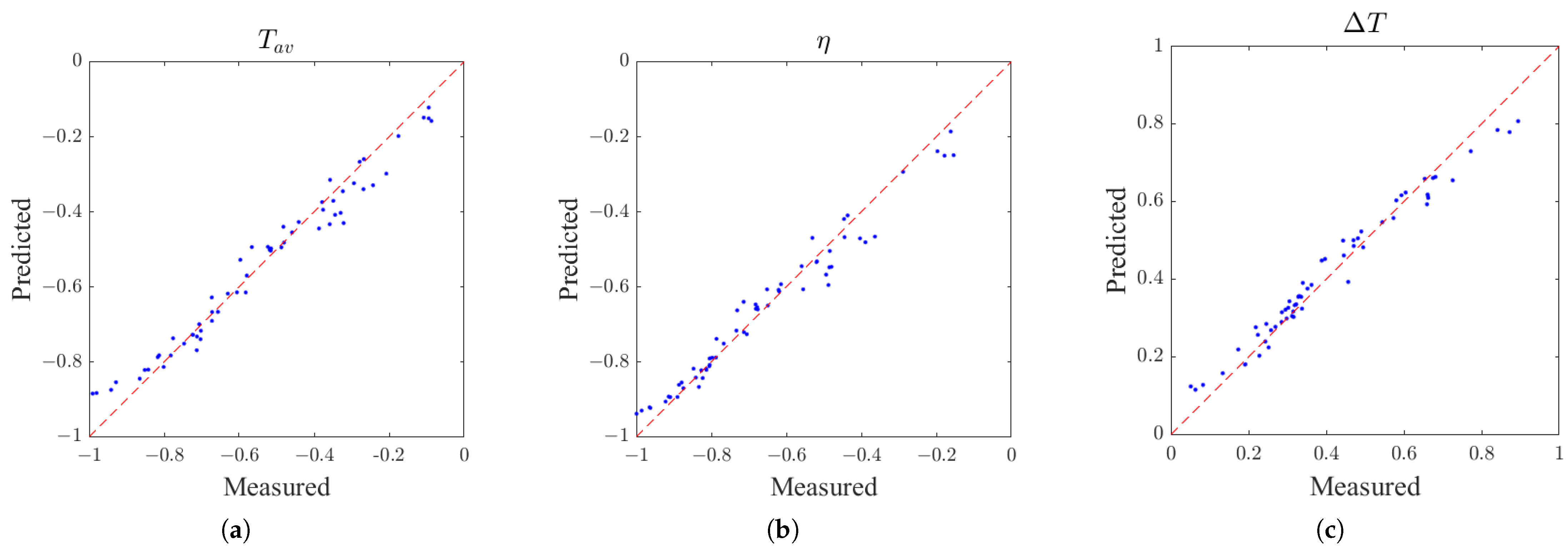
The proposed framework integrates three core components to systematically optimize IPMSM performance. First, a dual-strategy variable importance analysis combining RF and ANOVA is employed to identify key design parameters. RF focuses on the contribution of design variables to the model’s predictions, while ANOVA examines the sensitivity of design variables to optimization objectives, ensuring that the selected variables (flux barrier thickness $b_r$, PM thickness $b_m$, and PM width $l_m$) possess both predictive utility and high sensitivity. Next, a GRNN surrogate model is constructed using LHS optimized by the Morris–Mitchell criterion. GRNN’s single hyperparameter architecture simplifies training and enhances efficiency under limited samples, achieving high prediction accuracy ($R^2$ > 0.96). Finally, an MOPSO algorithm generates Pareto-optimal solutions, and an entropy-weighted distance metric objectively selects the final design by quantifying trade-offs between normalized objectives, eliminating reliance on subjective expert judgment.

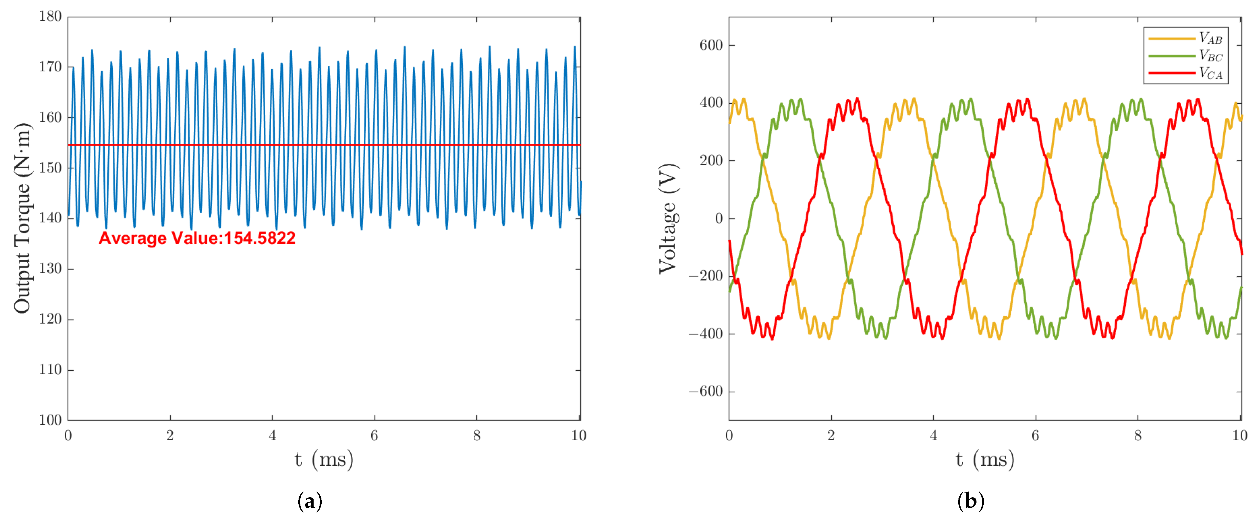
The optimized IPMSM demonstrates significant performance improvements over the prototype. Finite element analysis validates a 4.62% increase in average output torque (from 154.96 N·m to 162.12 N·m), a 0.15% enhancement in efficiency (from 98.05% to 98.20%), and a 10.48% reduction in torque ripple (from 36.13 N·m to 32.35 N·m). The surrogate model predictions align closely with simulation results, exhibiting relative errors below 2.92%, confirming the framework’s robustness. These enhancements are attributed to optimized magnetic flux concentration and reduced leakage through strategic adjustments to $b_r$, $b_m$ and $l_m$, validated by increased air gap flux density and improved pole-arc characteristics.

In conclusion, this study advances surrogate-assisted optimization for IPMSMs, providing a systematic, data-driven framework that balances computational efficiency, predictive accuracy and engineering practicality.

References

1. Yu, Y.; Liang, C.; Zeng, D.; Hu, Y.; Yang, J. Multi-objective optimization of IPMSM for electric vehicles based on the combinatorial surrogate model and the hierarchical design method. Int. J. Electr. Power Energy Syst. 2024, 162, 110245. [Google Scholar] [CrossRef]
2. Liu, F.; Wang, X.; Wei, H. Improved Multiphysics Multiobjective Optimization for U-Shaped IPMSM Equipped With Eccentric Rotor. IEEE J. Emerg. Sel. Top. Power Electron. 2023, 11, 5131–5144. [Google Scholar] [CrossRef]
3. Sun, X.; Shi, Z.; Lei, G.; Guo, Y.; Zhu, J. Multi-Objective Design Optimization of an IPMSM Based on Multilevel Strategy. IEEE Trans. Ind. Electron. 2021, 68, 139–148. [Google Scholar] [CrossRef]
4. Gu, J.; Hua, W.; Yu, W.; Zhang, Z.; Zhang, H. Surrogate Model-Based Multiobjective Optimization of High-Speed PM Synchronous Machine: Construction and Comparison. IEEE Trans. Transp. Electrif. 2023, 9, 678–688. [Google Scholar] [CrossRef]
5. Li, G.; Li, R.; Hou, H.; Zhang, G.; Li, Z. A Data-Driven Motor Optimization Method Based on Support Vector Regression—Multi-Objective, Multivariate, and with a Limited Sample Size. Electronics 2024, 13, 2231. [Google Scholar] [CrossRef]
6. Sato, H.; Igarashi, H. Fast Multi-Objective Optimization of Electromagnetic Devices Using Adaptive Neural Network Surrogate Model. IEEE Trans. Magn. 2022, 58, 1–9. [Google Scholar] [CrossRef]
7. Liu, Z.; Zhang, G.; Du, G. An Investigation of Parameter Dimension Reduction Optimization of PMA-Synrm. Appl. Sci. 2025, 15, 1529. [Google Scholar] [CrossRef]
8. McNeish, D.M.; Stapleton, L.M. The Effect of Small Sample Size on Two-Level Model Estimates: A Review and Illustration. Educ. Psychol. Rev. 2016, 28, 295–314. [Google Scholar] [CrossRef]
9. Hanic, Z.; Hanic, A.; Kovacic, M. The Application of Neural Network Metamodels Interior Permanent Magnet Machine Performance Prediction. In Proceedings of the 2021 International Conference on Electrical Drives & Power Electronics (EDPE), Dubrovnik, Croatia, 22–24 September 2021; pp. 118–122, ISSN 1339-3944. [Google Scholar]
10. Liu, X.; Li, X.; Huang, S. Parameters Optimization of the Permanent Magnet Linear Synchronous Machine Using Kriging-based Genetic Algorithm. In Proceedings of the 2019 22nd International Conference on Electrical Machines and Systems (ICEMS), Harbin, China, 11–14 August 2019; pp. 1–6, ISSN 2642-5513. [Google Scholar]
11. Seo, H.S.; Park, C.B.; Kim, S.H.; Lei, G.; Guo, Y.; Lee, H.W. Utilizing MicroGenetic Algorithm for Optimal Design of Permanent-Magnet-Assisted WFSM for Traction Machines. Appl. Sci. 2024, 14, 5150. [Google Scholar] [CrossRef]
12. Chai, J.; Zhao, T.; Gui, X. Design and Multi-Objective Optimization for Improving Torque Performance of a Permanent Magnet-Assisted Synchronous Reluctance Motor. World Electr. Veh. J. 2021, 12, 131. [Google Scholar] [CrossRef]
13. Yang, F.; Li, N.; Du, G.; Huang, M.; Kang, Z. Electromagnetic Optimization of a High-Speed Interior Permanent Magnet Motor Considering Rotor Stress. Appl. Sci. 2024, 14, 6033. [Google Scholar] [CrossRef]
14. Xing, F.; Zhang, J.; Zuo, F.; Gao, Y. Optimization of an Asymmetric-Rotor Permanent Magnet-Assisted Synchronous Reluctance Motor for Improved Anti-Demagnetization Performance. Appl. Sci. 2024, 14, 11233. [Google Scholar] [CrossRef]
15. Pei, W.; Xiao, P.; Pan, J.; Li, Z.; Lv, A. Multi-Objective Optimization Strategy for Commercial Vehicle Permanent Magnet Water Pump Motor Based on Improved Sparrow Algorithm. Appl. Sci. 2024, 14, 9666. [Google Scholar] [CrossRef]
16. Hsiao, C.Y.; Htet, S.M. Multi-Step Design Optimization for the Improvement of an Outer-Rotor Brushless Direct Current Motor. Appl. Sci. 2024, 14, 4302. [Google Scholar] [CrossRef]
17. Pan, Z.; Fang, S. Combined Random Forest and NSGA-II for Optimal Design of Permanent Magnet Arc Motor. IEEE J. Emerg. Sel. Top. Power Electron. 2022, 10, 1800–1812. [Google Scholar] [CrossRef]
18. Pan, Z.; Fang, S.; Wang, H.; Zhong, Y. Accurate and Efficient Surrogate Model-Assisted Optimal Design of Flux Reversal Permanent Magnet Arc Motor. IEEE Trans. Ind. Electron. 2023, 70, 9312–9325. [Google Scholar] [CrossRef]
19. Cheng, M.; Zhao, X.; Dhimish, M.; Qiu, W.; Niu, S. A Review of Data-Driven Surrogate Models for Design Optimization of Electric Motors. IEEE Trans. Transp. Electrif. 2024, 10, 8413–8431. [Google Scholar] [CrossRef]
20. Liu, X.; Peng, W.; Xie, L.; Zhang, X. Optimization of a Multi-Type PMSM Based on Pyramid Neural Network. Appl. Sci. 2023, 13, 6810. [Google Scholar] [CrossRef]
21. Cen, Y.; Shen, H.; Wang, X.; Wu, Y.; Du, J. Multi-Objective Optimization Analysis of Electromagnetic Performance of Permanent Magnet Synchronous Motors Based on the PSO Algorithm. Energies 2024, 17, 4637. [Google Scholar] [CrossRef]
22. Yu, Y.; Zhao, P.; Hao, Y.; Zeng, D.; Hu, Y.; Zhang, B.; Yang, H. Multi Objective Optimization of Permanent Magnet Synchronous Motor Based on Taguchi Method and PSO Algorithm. Energies 2022, 16, 267. [Google Scholar] [CrossRef]
23. Rahmani Fard, J.; Jamali Arand, S.; Hemmati, S. Optimal design of a yoke-less axial flux switching PM motor based on multi-objective PSO. COMPEL Int. J. Comput. Math. Electr. Electron. Eng. 2023, 42, 1248–1262. [Google Scholar] [CrossRef]
24. Yang, Q.; Zhang, W.; Zhao, C. Research on Torque Performance of Marine Hybrid Excitation Synchronous Motors Based on PSO Optimization of Magnetic Permeability Structure. J. Mar. Sci. Eng. 2024, 12, 1064. [Google Scholar] [CrossRef]
25. Balaci, A.T.; Suh, E.S.; Hwang, J. Systematic application of traffic-signal-control system architecture design and selection using model-based systems engineering and Pareto frontier analysis. Syst. Eng. 2024, 27, 931–954. [Google Scholar] [CrossRef]
26. Rao, R.; Lakshmi, R. Ranking of Pareto-optimal solutions and selecting the best solution in multi- and many-objective optimization problems using R-method. Soft Comput. Lett. 2021, 3, 100015. [Google Scholar] [CrossRef]
27. Zhang, T.; Wei, Z.; Wang, L.; Xue, Z.; Wang, S.; Wang, P.; Qi, B.; Yue, Z. Multi-objective optimization of composite stiffened panels for mass and buckling load using PNN-NSGA-III algorithm and TOPSIS method. Thin-Walled Struct. 2025, 209, 112878. [Google Scholar] [CrossRef]
28. Saeed, M.A.; Junejo, F.; Amin, I.; Tanoli, I.K.; Algarni, A.D.; Ahmad, S.; Ateya, A.A. A hybrid two stage Taguchi-regression-NSGA II-AHP-GRA, multi-objective optimization framework for sustainable straight slot milling of AZ31 magnesium alloy. Results Eng. 2025, 25, 104451. [Google Scholar] [CrossRef]
29. Shannon, C.E. A mathematical theory of communication. Bell Syst. Tech. J. 1948, 27, 379–423. [Google Scholar] [CrossRef]
30. Barberi, E.; Cucinotta, F.; Forssén, P.E.; Sfravara, F. DECI: A Differential Entropy-Based Compactness Index for Point Clouds Analysis: Method and Potential Applications. Eng. Proc. 2023, 56, 273. [Google Scholar] [CrossRef]
31. Chen, P. Effects of the entropy weight on TOPSIS. Expert Syst. Appl. 2021, 168, 114186. [Google Scholar] [CrossRef]
32. E, J.; Han, D.; Qiu, A.; Zhu, H.; Deng, Y.; Chen, J.; Zhao, X.; Zuo, W.; Wang, H.; Chen, J.; et al. Orthogonal experimental design of liquid-cooling structure on the cooling effect of a liquid-cooled battery thermal management system. Appl. Therm. Eng. 2018, 132, 508–520. [Google Scholar] [CrossRef]
33. Gregorutti, B.; Michel, B.; Saint-Pierre, P. Correlation and variable importance in random forests. Stat. Comput. 2017, 27, 659–678. [Google Scholar] [CrossRef]
34. Ye, X.; Wu, L.; Sun, C.; Wang, L.; Zhang, J. Approximate Modeling of Gear Torque of Permanent Magnet Synchronous Motor Based on Improved Latin Hypercube Sampling. In Proceedings of the 9th Frontier Academic Forum of Electrical Engineering, Xi’an, China, 25–27 August 2020; Chen, W., Yang, Q., Wang, L., Liu, D., Han, X., Meng, G., Eds.; Springer: Singapore, 2021; pp. 487–500. [Google Scholar]
35. Xiao, Q.; Wang, J.; Jiang, B.; Yang, W.; Yang, X. Multi-objective optimization of squirrel cage fan for range hood based on Kriging model. Proc. Inst. Mech. Eng. Part C 2022, 236, 219–232. [Google Scholar] [CrossRef]
36. Wang, X.; Ju, H.; Lu, J. Wind turbine airfoils optimization design by generalized regression neural network under small sample. J. Mech. Sci. Technol. 2023, 37, 217–228. [Google Scholar] [CrossRef]
37. Li, J.; An, L.; Cheng, Y.; Wang, H. Small Sample Sound Quality Prediction Method of Hy-Vo Chain Transmission System Based on Fuzzy Generation. Appl. Sci. 2024, 14, 3147. [Google Scholar] [CrossRef]
38. Gharibi, A.; Doniavi, E.; Hasanzadeh, R. A metaheuristic particle swarm optimization for enhancing energetic and exergetic performances of hydrogen energy production from plastic waste gasification. Energy Convers. Manag. 2024, 308, 118392. [Google Scholar] [CrossRef]
39. Nayak, J.; Swapnarekha, H.; Naik, B.; Dhiman, G.; Vimal, S. 25 Years of Particle Swarm Optimization: Flourishing Voyage of Two Decades. Arch. Comput. Methods Eng. 2023, 30, 1663–1725. [Google Scholar] [CrossRef]
40. Lu, T.; Hao, M.; Zhang, Z. Comprehensive Evaluation of Remote Tower Controllers’ Situation Awareness Level Based on the Entropy Weight Method (EWM)–TOPSIS–Gray Relational Analysis Model. Appl. Sci. 2025, 15, 2623. [Google Scholar] [CrossRef]
Figure 1. Flowchart of this study.
Applsci 15 04259 g001
Figure 2. Three-dimensional schematic of the motor.
Applsci 15 04259 g002
Figure 3. (a) Full FEM of prototype machine. (b) Mesh arrangement of FEM analysis.
Applsci 15 04259 g003
Figure 4. Under no load: (a) Phase EMF waveform. (b) Line EMF waveform.
Applsci 15 04259 g004
Figure 5. On load: (a) Output torque waveform. (b) Line EMF waveform.
Applsci 15 04259 g005
Figure 6. Schematic of design variables.
Applsci 15 04259 g006
Figure 7. Random forest modeling principle diagram.
Applsci 15 04259 g007
Figure 8. Random forest model evaluation and variable importance scores: (a) MSE convergence of the random forest model; (b) variable importance scores for average output torque; (c) variable importance scores for motor efficiency; and (d) variable importance scores for torque ripple.
Applsci 15 04259 g008
Figure 9. Sampling results of the optimized Latin hypercube design: (a) 3D spatial distribution of experimental points; (b) projection of experimental points on Dimension 1 and Dimension 2; (c) projection of experimental points on Dimension 1 and Dimension 3; and (d) projection of experimental points on Dimension 2 and Dimension 3.
Applsci 15 04259 g009
Figure 10. Basic structure of GRNN.
Applsci 15 04259 g010
Figure 11. Comparison of predicted and measured values for optimization objectives: (a) average output torque; (b) motor efficiency; and (c) torque ripple.
Applsci 15 04259 g011
Figure 12. Pareto frontier images: (a) Pareto frontier 3D image; (b) projection of Pareto frontier on T a v and η ; (c) projection of Pareto frontier on T a v and Δ T ; and (d) projection of Pareto frontier on η and Δ T .
Applsci 15 04259 g012
Figure 13. Relationship between 3D Pareto frontier and entropy-weighted distance.
Applsci 15 04259 g013
Figure 14. (a) Air gap flux density. (b) Harmonic components in air gap flux density.
Applsci 15 04259 g014