Research on Pressure Exertion Prediction in Coal Mine Working Faces Based on Data-Driven Approaches

Abstract

Coal is the main energy source in China, but coal mining is a high-risk industry, making the prevention and control of coal mining hazards an important topic. Constrained by the complexity and unpredictability of underground spaces, current research on coal mining disaster prevention and control technologies mainly focuses on the characteristics of overlying strata and the laws of mine pressure, resulting in significant deficiencies in accuracy. Given this, a data-driven pressure prediction method is proposed, which uses deep learning models to learn the patterns in existing data and generate the required predictions. This approach avoids the challenges of accurately extracting rock mass physical and mechanical parameters and geological structure modeling, thereby improving the accuracy of disaster prevention and control. The stage of working face pressure exertion is a period prone to disasters during coal mining. To achieve accurate prediction of working face pressure, the task is divided into three steps: the first step is to predict support resistance data ahead of the working face, the second step is to classify the pressure labels of coordinate units, and the third step is to predict the characteristic parameters of pressure exertion. Deep learning models were designed and trained separately for each of the three steps: For the first step, a deep Spatiotemporal sequence model was selected, and the trained model achieved a mean absolute error of 4.65 kN in prediction. For the second step, an image segmentation-based classification model was chosen, with the trained model reaching a classification accuracy of 97.77%. For the third step, a fusion model consisting of three LSTM (Long Short-Term Memory) networks was designed. The trained model achieved a mean absolute error of 0.17 for the dynamic pressure coefficient, a maximum resistance error of 810.93 kN during the pressure period, an error of 9.96 cycles for the pressure duration, and a classification accuracy of 92.35% for the pressure type. Simulating the actual situation of application scenarios, the input data for the second and third steps were set as the output data from the previous step, and the model was evaluated. The model achieved a mean absolute error of 1035.21 kN for the prediction of support resistance and classification accuracy of 82.90% for the pressure labels of coordinate units. In the simulated scenario, there were 9922 instances of pressure exertion, and the model predicted 10,336 instances, with 9046 of them matching the actual instances. The prediction of characteristic parameters was evaluated for 4946 instances of pressure exertion, which included three complete pressure exertion cycles. The mean absolute error for the dynamic pressure coefficient was 0.21, the maximum resistance error during the pressure period was 1218.31 kN, the error for the duration of the pressure cycle was 11.03 cycles, and the classification accuracy for the pressure exertion type was 91.75%.

1. Introduction

Coal is the primary energy source in China and plays a crucial role in the country’s primary energy consumption [1,2,3]. However, coal mining is a high-risk industry, and safety accidents still occur occasionally during the coal mining process, posing a threat to the lives of underground miners. To address this, measures such as the structural reform of the national energy supply side (phasing out small and medium-sized coal mines with low safety guarantees or outdated environmental protection facilities, accelerating the pace of mergers and acquisitions in the coal industry to increase industry concentration, and promoting the construction of smart mines), improving relevant laws and regulations on coal mine safety, and enhancing safety management levels have been implemented, achieving remarkable results [4,5,6]. Nevertheless, from the perspective of disaster prevention and control technology, the complexity and unknowns of underground spaces pose significant challenges to the precision of coal mine safety accident prevention and control, which restricts the further improvement of safe mining levels in coal mines.

During the process of coal mining at the working face, the overlying strata undergo periodic fracture, exhibiting a “stable-unstable-restabilized” process. The structural instability of the overlying rock mass leads to pressure exertion on the working face, which occurs periodically as the working face advances. During the period of pressure exertion, the overlying rock mass is in an unstable state, resulting in increased support resistance, prone coal wall spalling, and exacerbated roadway deformation, making it a period highly susceptible to safety accidents. Therefore, accurately predicting the pressure exertion at the working face is of great significance for ensuring safe coal mining.

Currently, research on the pressure exertion on the working face mainly employs a combination of theoretical analysis, physical simulation, numerical simulation, and on-site monitoring. Cai et al. [7] established a physically similar simulation model to analyze the impact of upper mining on the underlying coal seam and studied the deformation and failure patterns of the overlying rock mass as well as the stress distribution after upper mining. Li et al. [8] studied the roof fragmentation characteristics and ground pressure laws during close-distance coal seam mining through theoretical analysis, numerical simulation, and engineering verification. It was found that the roof exhibited a “loose block” structure, and the basic roof fracture spacing was 44.61 m. To reduce mining-induced disturbances in deep mining, Wang et al. [9] proposed a technique of full mining with partial backfilling. Using FLAC numerical simulation, the distribution pattern of mining-induced pressure on the working face was analyzed. Field measurements revealed that the initial supporting force of the support’s working resistance became more stable after adopting this technique. Zhou et al. [10] investigated the distribution law of mine ground pressure based on a microseismic system. It was found that microseismic monitoring could further analyze the destabilization process of the ore deposit caused by mining. The combination of surface subsidence, mining intensity, and energy release could verify the accuracy of stress distribution and ground pressure transmission. To study the mining pressure characteristics of shallow coal seams beneath extremely dense gob areas, Lan et al. [11] employed theoretical analysis to determine whether the cutting horizon’s bearing layer fell under such conditions. Based on FLAC3D numerical simulations and field measurements of the end-of-cycle resistance of supports, a method for classifying mining-induced stress according to the advancing length of the working face was proposed. Wang et al. [12] addressed the issue of abnormal pressure in isolated working faces of thin coal seams beneath residual coal pillars using a combination of theoretical analysis, numerical simulation, and field measurements. The study focused on the stress distribution pattern in the 33,107 isolated working faces. Wu et al. [13] analyzed the characteristics of roof caving and overburden fracture development in Xinjiang using physically similar simulation methods. Field monitoring revealed that the hydraulic support pressure was relatively low in shallow coal seams with thin bedrock, but the stability of the coal wall and roadways was good. Jia et al. [14] proposed an “umbrella arch” overburden structure for isolated working faces with hard roofs and derived an expression for the initial supporting force of the supports under these conditions. This theoretically established the correspondence between the near-gob area and the isolated working face. Numerical simulations were used to understand the variation in peak elastic energy difference on the solid coal side of the transport and extraction roadways in irregular island-shaped working faces. In summary, previous methods mainly focused on studying overburden characteristics and ground pressure laws and had limited accuracy in predicting incoming pressure. This was primarily due to difficulties in accurately extracting rock mass physicomechanical parameters and modeling geological structures.

Given the current research progress in extracting rock mass physicomechanical parameters and geological structure modeling, it is extremely challenging to improve the accuracy of pressure prediction by solving these issues. The development of big data and artificial intelligence technologies has led to the emergence of data-driven research methods. These methods focus on data, utilizing AI technologies to deeply analyze and mine big data, uncovering potential laws and patterns within the data to guide scientific research, product development, or decision-making. This approach only requires inputting existing information and, based on the learned correlation between existing information and the information to be predicted, it can generate prediction results, thereby bypassing the processes of extracting rock mass physicomechanical parameters and geological structure modeling. Furthermore, since data are objective and not influenced by researchers’ subjective factors, predictions driven by data are more objective and accurate. According to surveys, data-driven research has already been conducted in fields such as real-time prediction of shield tunneling machine posture and position [15], drug design [16], metal additive manufacturing [17], PM2.5 prediction [18], monthly traffic flow prediction [19], mechanical fatigue life prediction [20], and landslide prediction [21]. This has become a current research trend, aligning with the national call for deep integration of AI into various industries.

Data-driven prediction of pressure exertion in working faces has been explored in previous studies, primarily focusing on the prediction of support resistance, which is the foundation for predicting pressure exertion. Building on these works, this paper will systematically investigate data-driven methods for predicting pressure exertion in working faces, breaking through the bottleneck of improving prediction accuracy under existing research paradigms. It aims to provide relevant methods and theories for coal mine safety mining technologies in the era of big data and artificial intelligence.

2. Materials and Methods

2.1. Modeling of Pressure Exertion Prediction in Working Faces Driven by Data

The content of data-driven pressure exertion prediction in working faces includes advanced cycle support resistance data, pressure labels, and pressure exertion characteristic parameters (including the maximum support resistance during the pressure exertion period, dynamic pressure coefficient, duration of pressure exertion, and type of pressure exertion). This problem adopts a grid-based modeling approach, specifically considering support resistance data from multiple measurement lines and cycles in the working face, to establish a grid-based model for the entire working face area with support numbers and coal cutting cycles as the coordinate units, as shown in Figure 1. In this model, the characteristic value of each grid unit is defined as the working resistance of that support cycle, and the end resistance of the support cycle is particularly selected as the key characteristic value.

Under this modeling approach, the prediction of pressure exertion in the working face can be divided into three steps. The first step is the prediction of support resistance data, which serves as the foundation for solving and predicting pressure exertion parameters in the working face. By inputting known information, the deep learning model obtains the support resistance data based on the correlation between the known information and the support resistance. The second step is the classification of pressure labels for coordinate units. By predicting the end resistance values of the support cycles in the advanced coordinate units, the pressure labels are classified to determine whether the coordinate unit is experiencing pressure exertion. The third step is the prediction of pressure exertion characteristic parameters. Solving for these parameters requires obtaining complete stage support resistance information for a given pressure exertion event, but the predicted advanced range of cycles often only captures the first few cycles of the pressure exertion. To provide accurate pressure exertion characteristic parameters to the site after predicting that a pressure exertion event is about to occur, allowing for more targeted measures to be taken, a deep learning model needs to be designed to predict these parameters based on the information from existing cycles.

2.2. Method for Solving Pressure Exertion Characteristics Based on Historical Data

The solution of pressure exertion characteristics refers to the two tasks of determining the location of pressure exertion and solving for the characteristic parameters of pressure exertion based on the real support resistance data obtained after mining. This forms the foundation for establishing the dataset for the prediction work discussed in this paper. The determination of pressure exertion location is achieved through the classification results of pressure labels for coordinate units. Once the location of pressure exertion is known, the characteristic parameters of pressure exertion can be directly obtained through formulas. Therefore, the core issue in solving pressure exertion characteristics lies in the classification of pressure labels for coordinate units.

For a long period of time, the method based on discriminant formulas under a single measurement line has been used for the classification of pressure labels for coordinate units. However, this method suffers from three issues: the empirical coefficients of the discriminant formulas are difficult to determine, the results of pressure labeling are not continuous, and it is challenging to grasp the overall pressure exertion pattern in the working face. To address these problems, after establishing a grid model of the entire working face with support numbers and coal-cutting cycles as the coordinate units, the author of this paper designed a method based on spatiotemporal feature clustering of support resistance for coordinate units. Specifically, a coordinate unit is taken as a sample unit, and the sample feature values are derived from the feature values of 25 adjacent coordinate units. These 25 coordinate units encompass the spatiotemporal characteristics of the pressure exertion state of the sample coordinate unit. Through k-means spatiotemporal clustering, continuous classification of pressure labels is achieved. Based on the continuous classification results of pressure labels, the author of this paper developed a program for solving the location and characteristic parameters of pressure exertion, enabling a fully automated solution of these parameters [22].

2.3. Method for Predicting Support Resistance Data

This is the first step in predicting pressure exertion in the working face, which involves forecasting the support resistance data for advanced cycles. This is a crucial aspect of data-driven pressure exertion prediction in the working face and significantly affects the accuracy of the prediction. It is currently one of the most extensively researched areas. Support resistance is correlated with various modes of input data, including historical support resistance data, data reflecting overburden activity, and data reflecting the geological conditions of the mining face. By inputting these types of data, predictions of support resistance data can be achieved. Current research on support resistance prediction mainly focuses on predictions based on historical support resistance data, and this paper also only considers prediction results based on historical support resistance data.

For a long time, support resistance prediction based on historical information has been grounded in the temporal correlation of support resistance data, utilizing deep time series models represented by LSTM (Long Short-Term Memory) and GRU (Gated Recurrent Unit), as evidenced in the research by Zhao Yixin [23], Yang Zhiping [24], Liu Yixin [25], and others. In recent years, researchers have discovered that the spatial correlation of support resistance data is crucial for prediction results, and they have attempted to improve prediction performance by extracting spatial correlation while modeling the temporal correlation of support resistance data. Miao Yunfeng [26], Li Zemeng [27], and others have explored methods that combine machine learning algorithms to extract spatial correlation with deep time series models to extract temporal correlation. However, deep learning has been proven to outperform machine learning, which is a limitation of this approach. Gao et al. [28] employed an adaptive graph convolutional neural network to extract the spatiotemporal relationship of support resistance data, resulting in a significant reduction in prediction error. Based on these studies, we propose a support resistance prediction method based on a deep spatiotemporal sequence model. This model uses a convolutional neural network to extract spatial features, which excels in processing grid data with spatial correlation, such as images [29,30,31], and a recurrent neural network to extract temporal features, which is adept at handling sequence data with temporal dynamic information, such as text [32]. By integrating the two, the deep spatiotemporal sequence model addresses the challenge of unified modeling of spatiotemporal features, making it highly suitable for support resistance prediction. Experiments have demonstrated its advantages in this context [33]. In the first stage of support resistance prediction, we will select the PredRNN(Predictive RNN) deep spatiotemporal sequence model, which achieves the best experimental results. The detailed structure of the PredRNN model will not be repeated here and can be found in the relevant literature [33,34].

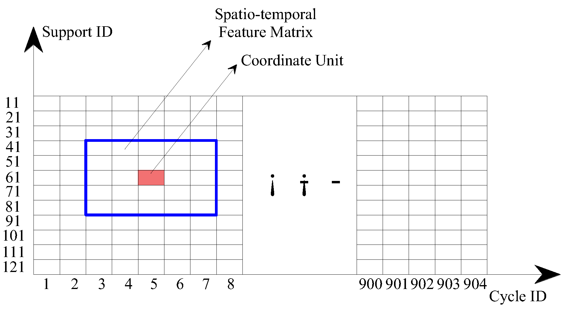
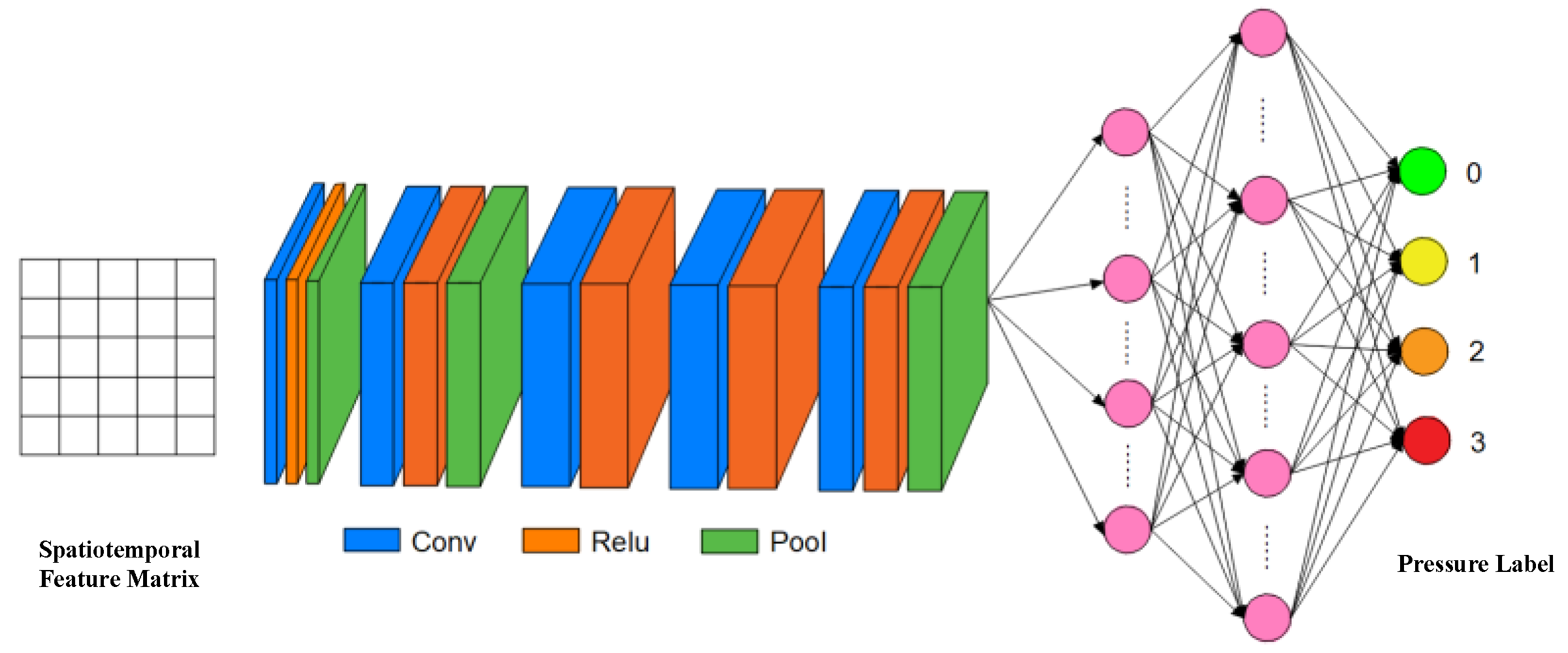
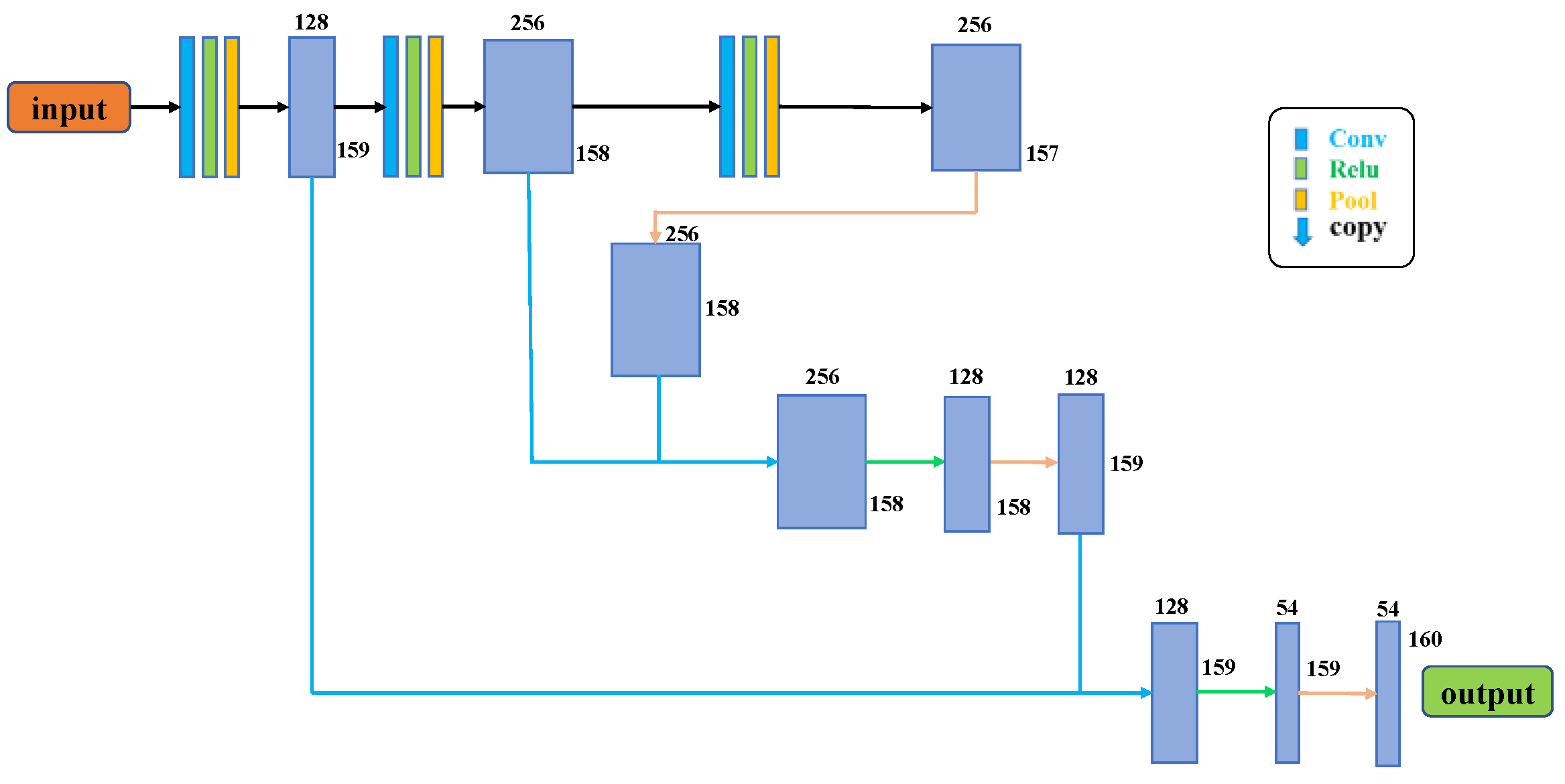
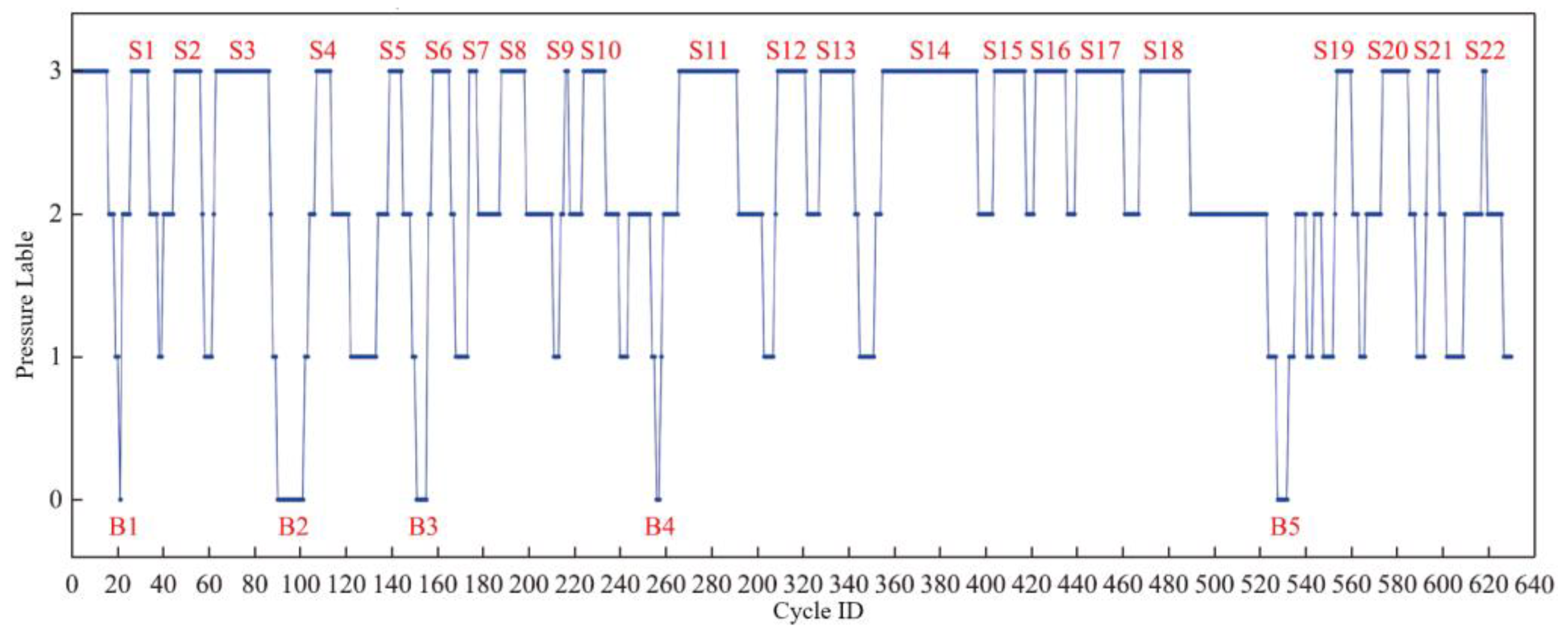
2.4. Real-Time Classification Method for Pressure Labels of Coordinate Units

This is the second step in predicting pressure exertion in the working face, which involves classifying pressure labels for coordinate units based on predicted support resistance data. Section 2.2 discussed a classification method for pressure labels using historical data, which employs clustering algorithms to categorize labels based on differences between samples, relying on a large number of data samples. However, the predicted support resistance data samples are limited, making it difficult to achieve classification through this unsupervised algorithm. Establishing a supervised classification model using deep learning, which learns the correlation between sample input features and classification labels through model training, enables the model to automatically discern the classification label for each cycle of support resistance prediction results. This is an effective modeling approach for the second step.

There are two deep-learning modeling schemes in this step, and their performances need to be compared experimentally to determine the optimal choice. Scheme ① is as follows: each support coordinate unit is considered as a prediction sample, where the input data are the spatiotemporal feature matrix of the support resistance for that particular support cycle, and the output data are the corresponding pressure label value. This modeling approach transforms the problem into an image-level classification problem, where the feature learning content of the model aligns with the classification method for pressure labels based on all historical data, ensuring the validity of the classification. In this modeling scheme, the input image size is 5 × 5, and the number of output classification labels is 4, with a computational complexity lower than that of handwritten digit recognition. Therefore, the AlexNet model can meet the modeling performance requirements for this problem [35]. Adjustments have been made to the AlexNet model structure to accommodate the input and output data sizes. The adjusted model structure is shown in Figure 2. The model consists of five convolutional layers and three fully connected layers. The 1st, 2nd, and 5th convolutional layers are followed by activation layers and pooling layers, while the 3rd and 4th convolutional layers are only followed by activation layers. The model hyperparameters are as follows: the convolutional kernel size is 3 × 3, the stride is 1, the pooling type is max pooling, the learning rate is 0.001, the optimizer is Adam, and the Dropout rate is 0.5.

Scheme ② involves constructing a feature matrix for the classification model using all predicted stent resistance values for advanced coordinate units, with each feature matrix representing a prediction sample. This modeling approach transforms the problem into a pixel-level classification issue within the field of image segmentation, effectively addressing the coupling of global and local features, although its effectiveness remains unknown. The FCN (Fully Convolutional Network) model converts the fully connected layers of an image classification network into convolutional layers, forming a fully convolutional neural network that enables end-to-end training. Through deconvolution for upsampling and the use of skip architectures to combine semantic and representational information, it produces accurate and precise segmentation. Recognized as a pioneering work in the field of semantic segmentation, the FCN model can meet the performance requirements of this modeling approach [36,37]. Adjustments have been made to the FCN model structure to accommodate the input and output data dimensions. The adjusted model structure is shown in Figure 3. The model hyperparameters are as follows: the convolutional kernel size is 3 × 3, the stride is 1, the pooling type is max pooling, the learning rate is 0.001, the optimizer is Adam, and the Dropout rate is 0.5.

2.5. Method for Predicting Pressure Exertion Characteristic Parameters

This is the third step in predicting pressure exertion at the working face. In this step, based on the pressure label classification results from the second step, the pressure exertion cycles are determined, and the characteristic parameters indicating the onset of pressure exertion are predicted. After obtaining the pressure labels for each coordinate unit, the maximum values for all survey line coordinate units within the same mining cycle are taken to derive the cyclic pressure label distribution curve, with Figure 4 serving as a schematic representation of the curve. According to the “stable-unstable-restabilized” characteristics of the overlying rock mass during periodic pressure exertion events, the information for one pressure exertion event consists of curve data from three stages: the first stage, where the overlying rock mass and the working face are in a completely stable state, comprising cycles labeled as 0, as shown by B1 to B5 in the figure; the second stage, which represents the process from the cycle label decreasing to a relative minimum between two pressure exertion events and then rising again to the maximum, indicating the transition of the overlying rock mass and the working face from a relatively stable state to instability and subsequently to another pressure exertion event at the working face; and the third stage, where the working face is under pressure exertion, comprising cycles labeled with the maximum value, as shown by S1 to S22 in the figure.

The data from the three stages encompass the complete information of a single pressure exertion event, and the characteristic parameters of the pressure exertion can be solved through formulas based on this information. Deep learning, through multi-layer nonlinear transformations, can learn high-level abstract representations of data, thereby representing complex functional relationships. Therefore, these formulas can be replaced by deep learning models to obtain pressure exertion characteristic parameters by inputting the information from the three stages. The challenge here lies in the fact that the information from these three stages is not always complete. The application scenario here expects to predict the required pressure exertion characteristic parameters based on the available information as much as possible when the information is incomplete, which is the main reason for replacing the formulas with deep learning models. To this end, a fusion model with three-stage feature fusion, as shown in Figure 5, is designed. This model consists of three LSTM networks, each representing one of the three stages of a pressure exertion event in the cyclic pressure label distribution curve. After learning the information from each stage separately, the three-stage information is fused through a fully connected layer to generate the final pressure exertion characteristic parameters. The model hyperparameters are as follows: The hidden layer size is 256, the learning rate is 0.001, the optimizer is Adam, and the Dropout rate is 0.5.

3. Results and Discussion

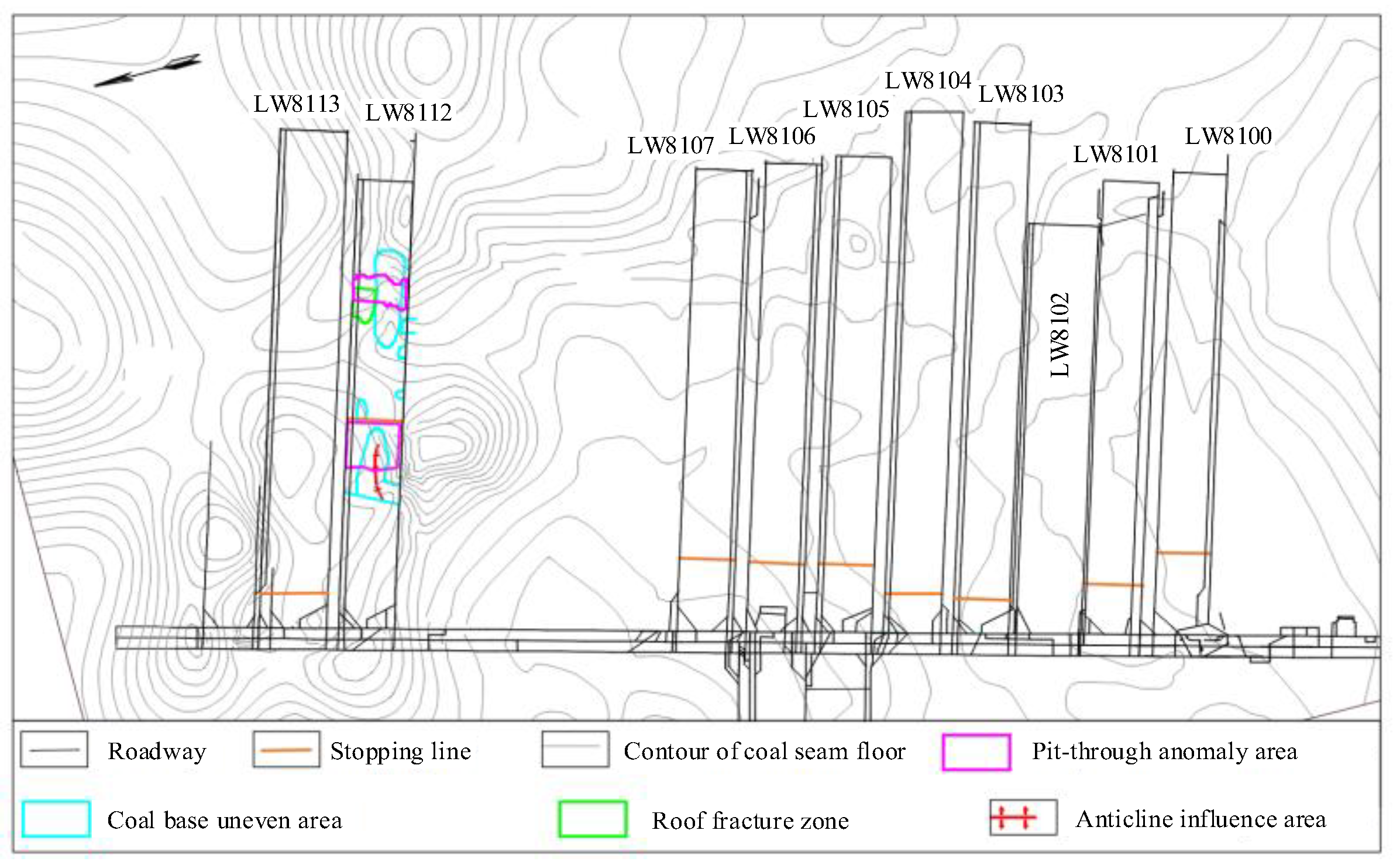
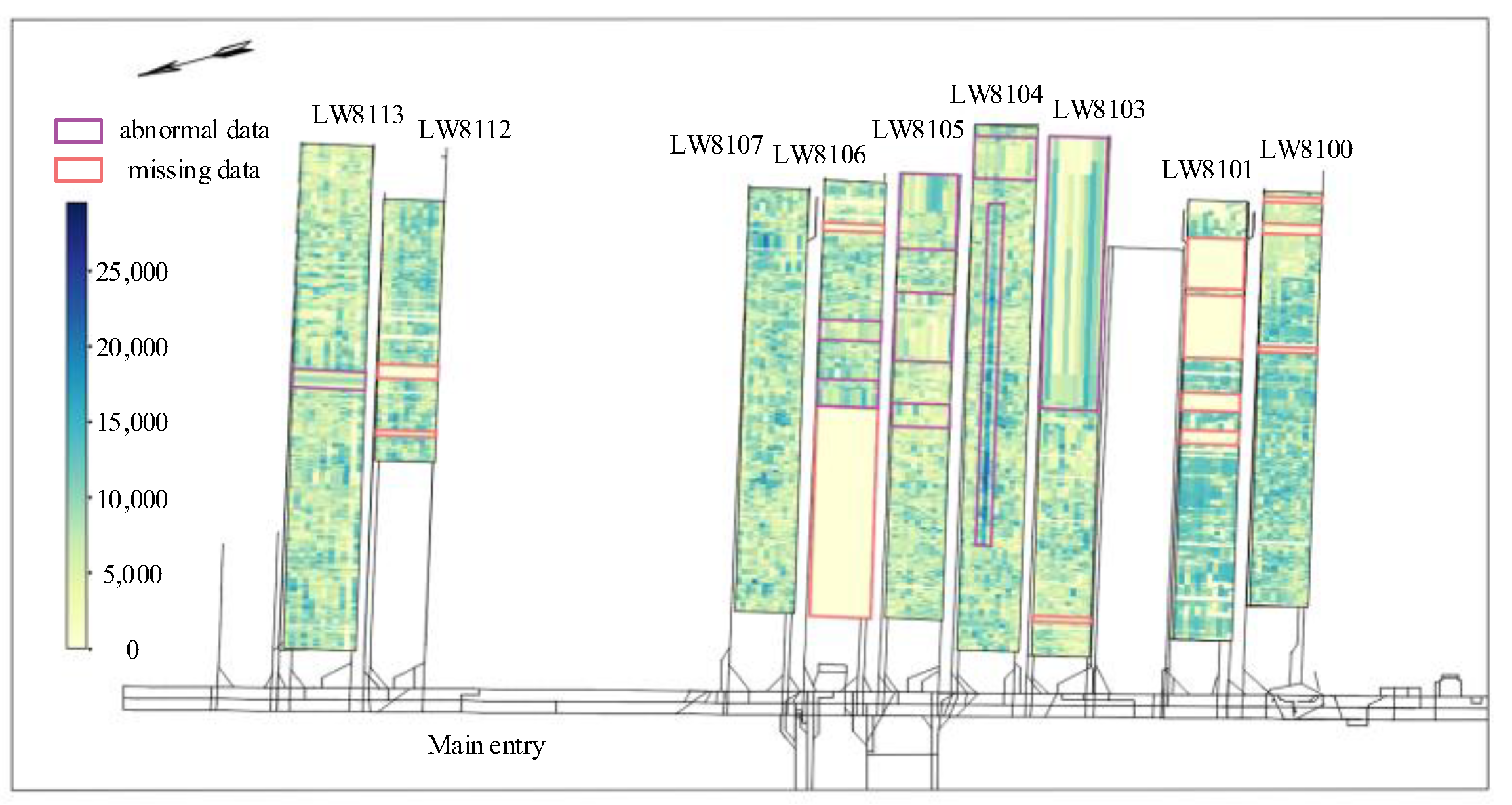
3.1. On-Site Data Acquisition and Preprocessing

Data collection and acquisition were conducted at a mine in the Datong Mining Area. This work encompassed support resistance data from 10 working faces, whose distribution is shown in Figure 6, and the mining statistics are summarized in

Table 1. Statistics of mining conditions for data acquisition working faces.

Workface Name	Extraction Sequence	Start Time	End Time	Strike Length/m	Mining Situation of Adjacent Workface in the Same Level
LW8100	②	2010.10	2011.07	1413.26	one side gob
LW8101	①	2009.10	2010.10	1500.93	first mining face
LW8102	⑩	2020.03	2021.08	1516.55	bilateral coal
LW8103	⑦	2014.02	2015.03	1773.49	one side gob
LW8104	⑥	2013.07	2014.05	1793.30	one side gob
LW8105	⑤	2012.11	2013.07	1521.77	one side gob
LW8106	③	2011.07	2012.03	1448.79	bilateral coal
LW8107	④	2012.03	2012.11	1449.52	one side gob
LW8112	⑨	2017.03	2018.05	891.86	one side gob
LW8113	⑧	2015.03	2016.06	1724.93	bilateral coal

. Among them, the LW8102 working face is currently being mined, and support resistance data from this face were collected over a period of approximately 7 months. This working face employs the latest electro-hydraulic control system, allowing for the precise acquisition of end-of-cycle support resistance values. The heatmap distribution of this part of the support resistance data is shown in Figure 7. The other nine working faces have already been mined, and complete historical support resistance data for these nine faces was collected. Since these data consist of support resistance values recorded every 5 min, data cleaning was performed using Kettle 9.1 software, and a program was written to extract end-of-cycle support resistance, resulting in the heatmap distribution of support resistance data shown in Figure 8.

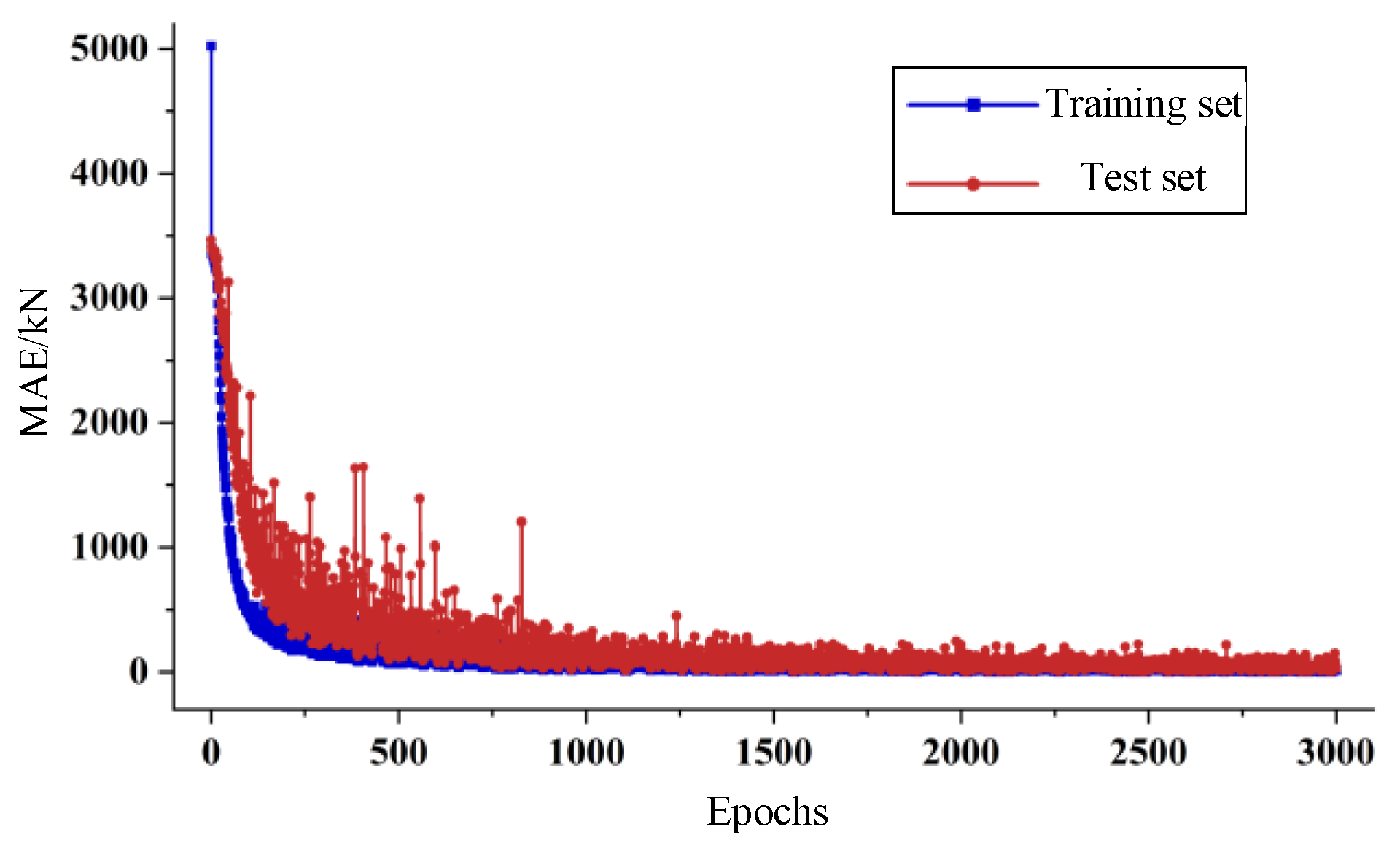
3.2. Training of Support Resistance Prediction Model

In the first step, the PredRNN deep spatiotemporal sequence network is selected as the support resistance prediction model. The support resistance spatiotemporal feature matrix of the research coordinate unit is formed by itself and its surrounding 24 coordinate units, as shown in Figure 9. By stacking the support resistance spatiotemporal feature matrices of 14 measuring lines in the research cycle, the support resistance spatiotemporal feature matrix of the research cycle is constructed, with a sample feature shape of 5514 for each timestamp. The model is trained by inputting 50 cycles of support resistance data to predict the support resistance data for the next 30 cycles.

The dataset is based on LW8102 data, with the training set accounting for 80% of the total samples and the test set accounting for 20%. Data collection efforts in LW8102 resulted in a total of 630 cycles of support resistance data. Since the model requires 50 cycles of input data and outputs 30 cycles of data, the dataset comprises 550 samples. By setting a random number, the samples are divided into a training set of 440 and a test set of 110.

During the training process, the model evaluated the prediction error of support resistance, specifically the MAE (Mean Absolute Error) values between the predicted data and the actual data for both the training and test sets, as shown in Figure 9. The figure indicates that the errors for both the training and test sets significantly decrease with the increase in training epochs, demonstrating that support resistance data can be predicted based on the correlation between historical and future information. Throughout the training process, the error for the test set consistently exceeds that of the training set, with a more pronounced difference in the first 1000 epochs. As the training epochs increase, the gap between the two errors gradually narrows, indicating that the model exhibits a certain degree of overfitting, which is mitigated by increasing the number of training epochs. The optimal training result is achieved at the 2485th epoch, with a training set error of 1.83 kN and a test set error of 4.65 kN.

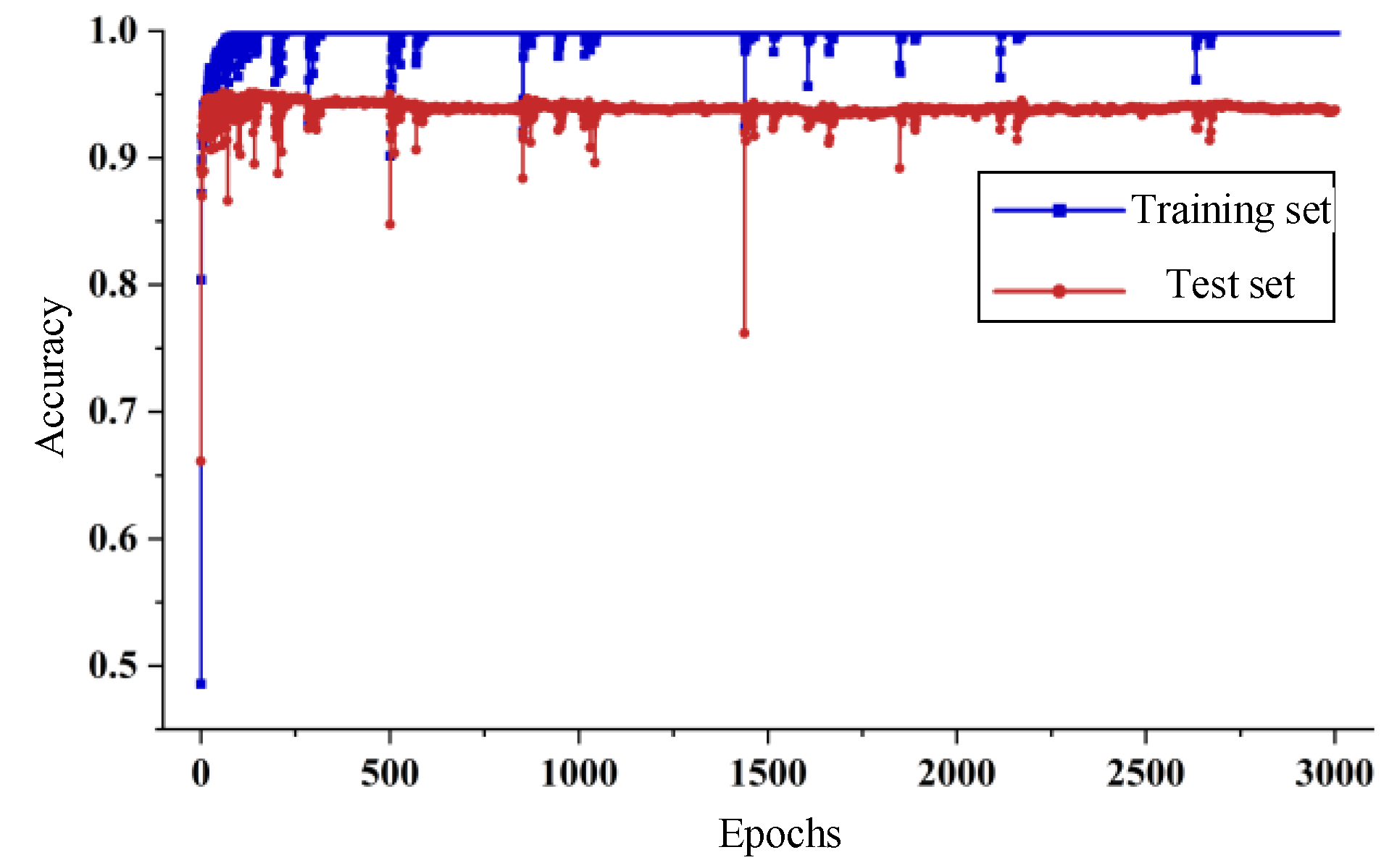
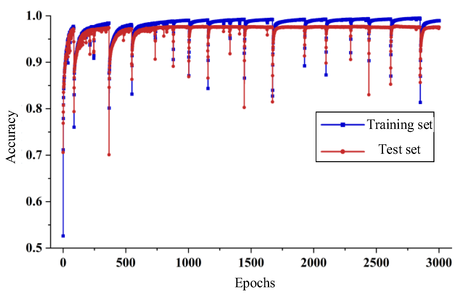
3.3. Training of Coordinate Unit Pressure Label Classification Model

In the second step, experiments were conducted on the prediction models under both schemes using the LW8102 dataset as the foundation. For Scheme ①, there were a total of 8820 data samples. A random number was set to divide the dataset into a training set accounting for 80% and a test set accounting for 20%, resulting in 7056 samples in the training set and 1764 samples in the test set. The curve of accuracy changes in the test set and training set during model training is shown in Figure 10. As can be seen from the figure, the classification accuracy for both the training and test sets was monitored, with the variation curve over training epochs shown in Figure 10. As can be seen from the figure, the classification accuracy for both the training and test sets significantly increased with the increase in training epochs, with the training set achieving 100% accuracy at the 153rd epoch. Throughout the training process, the accuracy of the test set was always lower than that of the training set, indicating a certain degree of overfitting in the model. At the 60th epoch, the model achieved the highest accuracy for the test set, representing the optimal training result, with a training set accuracy of 98.97% and a test set accuracy of 95.13%.

For Scheme ②, there were a total of 550 data samples. A random number was set to divide the dataset into a training set accounting for 80% and a test set accounting for 20%, resulting in 440 samples in the training set and 110 samples in the test set. The curve of accuracy changes in the test set and training set during model training is shown in Figure 11. As can be seen from the figure, the classification accuracy of both the training and test sets significantly increased with the increase in training epochs, with the training set achieving a maximum accuracy of 99.53% at the 2842nd epoch. During the training process, the accuracy of the test set was slightly lower than that of the training set, indicating a certain degree of overfitting in the model. However, compared to the overfitting observed in Scheme ①, there was a significant improvement. At the 2658th epoch, the model achieved the highest accuracy for the test set, representing the optimal training result, with a training set accuracy of 99.38% and a test set accuracy of 97.77%. The model was better able to accurately classify pressure labels based on real-time stent resistance data.

In conclusion, the pressure label classification model based on image segmentation outperforms the model based on image classification in terms of prediction accuracy, generalization ability, and computational resources required, making it a superior modeling approach.

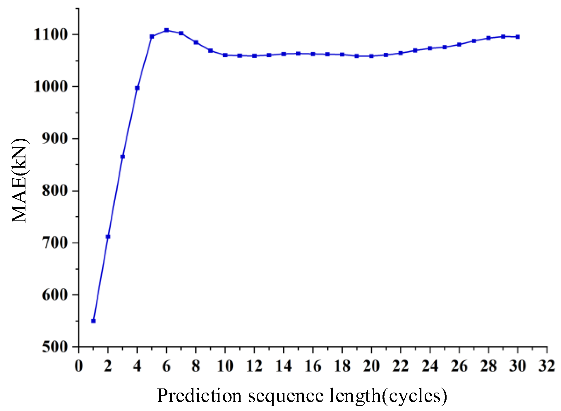
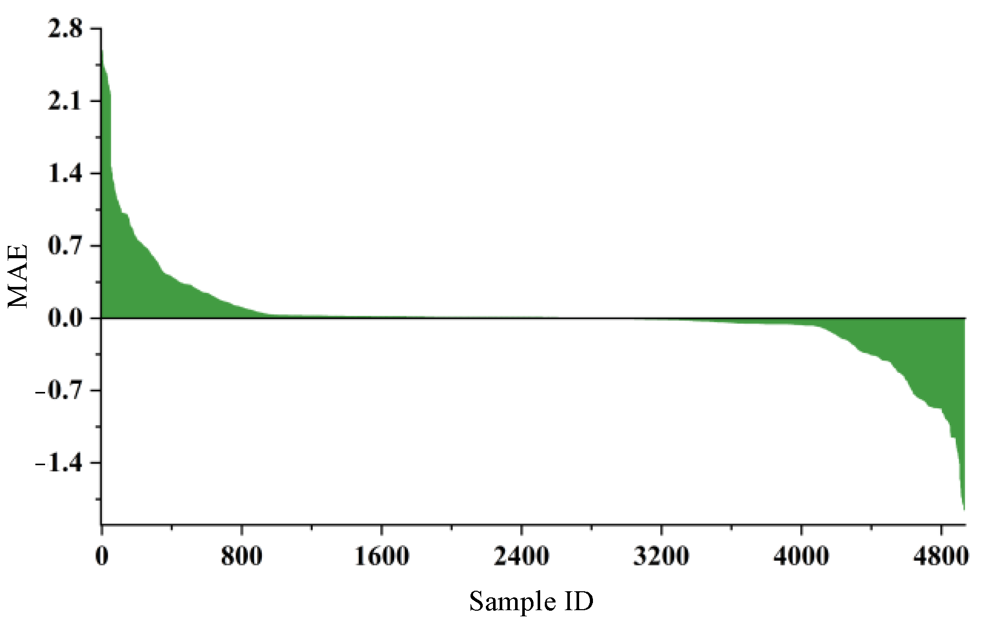
3.4. Training of the Predictive Model for Pressure Exertion Characteristic Parameters

To ensure a sufficient dataset, the model training in the third step was based on data collected from nine working faces. Using the method for solving pressure exertion characteristics from historical data described in Section 2.2, a total of 92 pressure exertions were identified, with the statistics summarized in

Table 2. Statistics of the observed pressure exertion situations.

Workface ID	Pressure Exertion Location (Cycle ID)	Number of Pressure Exertions
8100	300, 319, 358, 409, 473	5
8103	1902, 1962	2
8104	224, 245, 259, 329, 341, 406, 472, 489, 521, 597, 648, 687, 695, 763, 801, 810, 930, 952, 1283, 1361, 1402, 1415, 1557, 1588, 1608, 1700, 1742, 1761, 1797, 1823, 1972, 2043, 2082, 2119	34
8105	899	1
8106	234, 292, 340, 434, 471, 515, 539	7
8107	1426, 1459, 1537, 1600, 1621, 1625, 1662, 1737	8
8113	43, 90, 124, 171, 188, 194, 283, 297, 371, 412, 451, 512, 549, 588, 653, 673, 686, 746, 854, 989, 1035, 1054, 1097, 1107, 1115, 1128, 1166, 1232, 1497, 1538, 1608, 1636, 1642, 1661, 1705	35

. Among these 92 pressure exertions, some did not include all three complete stages of pressure exertion. Therefore, only those with all three stages were used to establish the dataset. Since, in actual prediction, the data for each stage of pressure exertion increases with the number of support cycles, the dataset gains an additional sample for each additional support cycle in the pressure exertion stage. The number of samples for a single pressure exertion corresponds to the number of support cycles it contains. When dividing the dataset, a random number was set to split it into a training set accounting for 80% of the total pressure exertions and a test set accounting for 20%, resulting in a training set of 2363 samples and a test set of 549 samples.

In the network shown in Figure 5, the support resistance data from 12 measurement lines within one support cycle constitutes the input data for a single timestamp. The number of support cycles contained in each stage of pressure exertion varies. According to statistics, the dataset samples contain a maximum of 23 support cycles in the stable stage, 57 in the unstable movement stage, and 236 in the pressure exertion stage. To ensure sufficient scalability of the model structure, the number of timestamps is set to 32 for the stable stage, 54 for the unstable movement stage, and 256 for the pressure exertion stage. When the number of support cycles is less than the number of timestamps, zero padding is used.

To analyze the impact of missing pressure exertion stages on prediction results and enable the prediction of pressure exertion characteristic parameters for cases lacking all three complete stages, the model was trained with four different input data scenarios: the pressure exertion stage alone, the unstable movement stage plus the pressure exertion stage, the stable stage plus the unstable movement stage plus the pressure exertion stage, and the unstable movement stage alone. The model was trained separately for each of these scenarios. During the training process, the prediction accuracy for both the training set and the test set was monitored, and the optimal prediction results for the test set under each scenario were recorded. These results are summarized in

Table 3. Statistics of optimal training results under different input information scenarios.

Input	Dynamic Pressure Coefficient		Error of Maximum Resistance		Error of Duration		Accuracy for Pressure Exertion Type
	Epochs	MAE	Epochs	MAE/kN	Epochs	MAE/Cycles	Epochs	Acc/%
“Third stage”	513	0.23	221	1137.51	144	10.45	204	76.14
“Second stage” +“Third stage”	12	0.24	34	977.93	963	11.58	813	78.32
“First stage” +“Second stage” +“Third stage”	927	0.17	48	810.93	32	9.96	73	92.35
“Second stage”	324	0.23	37	947.05	61	23.92	608	58.65

.

As can be seen from Table 3, when the input information includes three complete stages, the prediction accuracy for all four pressure exertion characteristic parameters is the highest, making it the optimal model. The optimal prediction results of this model for the four characteristics are as follows: the error for the dynamic pressure coefficient is 0.17, the error for the maximum resistance during pressure exertion is 810.93 kN, the error for the number of continuous cycles during pressure exertion is 9.96 cycles, and the accuracy for predicting the type of pressure exertion is 92.35%. The model achieves accurate predictions for all four pressure exertion characteristic parameters. When the first stage data are missing, the optimal input data for predicting the dynamic pressure coefficient is either the third or second stage, with both models having an error of 0.23; the optimal input data for predicting the maximum resistance is the second stage, with an error of 947.05 kN; the optimal input data for predicting the number of continuous cycles is the third stage, with an error of 10.45 cycles; and the optimal input data for predicting the type of pressure exertion is the combination of the “second stage + third stage”, with a prediction accuracy of 78.32%.

3.5. Pressure Exertion Prediction Based on Pre-Trained Models

In practical applications, the support resistance data for the next 30 cycles are first predicted based on the support resistance data from the previous 50 cycles. Then, the predicted support resistance data for the 30 cycles are input into the pressure label classification model. Based on the classification results, the input support resistance data for the pressure exertion characteristic parameters are extracted to obtain the required parameters. The above is the model training and evaluation result based on actual measured support resistance. In this section, the above model is used as a pre-trained model to simulate practical application scenarios and evaluate the model’s prediction performance.

The simulation scenario is based on the historical support resistance data collected from nine working faces. First, the support resistance data are predicted by sequentially increasing the support cycle number. The input data consist of the support resistance data from the previous 50 cycles, and the output data are the support resistance data for the next 30 cycles. If there are missing or abnormal values in the support resistance data for these 80 cycles, they are not included in the analysis sample. When constructing the support resistance feature matrix, the support resistance data from the two cycles before and after the target cycle is required. Therefore, in practical applications, only the support resistance data for the next 28 cycles can be predicted. This paper also includes the pressure exertion status of the current support cycle in the analysis, as the characteristics of the pressure exertion also need to be predicted if the current cycle is under pressure exertion. Therefore, a total of 29 support cycles’ pressure exertion characteristics need to be analyzed.

When predicting the pressure exertion characteristic parameters, the predicted support resistance data for 30 cycles are input into the pressure label classification model to obtain the pressure labels for those 30 cycles. The pressure labels for the last 28 cycles are then concatenated with the historical cycle pressure labels, and the maximum value for each cycle is taken to obtain the periodic pressure exertion characteristic distribution curve. The last 29 cycles of the periodic pressure exertion distribution curve are the 29 cycles that need to be analyzed. If any of these 29 cycles are under pressure exertion, the start cycle of the pressure exertion, as well as the start and end cycle numbers for the three stages of the pressure exertion, can be obtained from the curve.

Here, only pressure exertions that include three complete stages are analyzed. When data for three complete stages are not available, the characteristic value for that pressure exertion is defined as −1. Next, the predicted pressure exertions are matched with the actual pressure exertions. If the difference in the starting cycle between the two is less than two cycles, it indicates that the pressure exertion has been accurately predicted. The support resistance data for the three stages are then input into the pressure exertion characteristic parameter prediction model to obtain the four characteristic parameters. The prediction results during the simulation process are as follows:

(1)

Support resistance

In the simulation process, the support resistance for 8149 cycles was predicted, with an average prediction error of 1035.21 kN. The prediction error for different prediction sequence lengths is shown in Figure 12. As can be seen from the figure, the prediction error is smaller when the prediction sequence length is less than 4 and shows an increasing trend as the prediction sequence length increases. When the prediction sequence length is greater than 4, the prediction error tends to remain constant. The model’s prediction error is significantly affected by changes in the prediction sequence length. Compared with the results under the test set shown in Figure 9, the average prediction error of the model has increased from 4.65 kN to 1035.21 kN, indicating a significant increase in prediction error and suggesting that the model’s generalization ability still needs to be improved.

(2)

Pressure label

During the simulation process, pressure labels for 2,933,640 coordinate units were classified with an accuracy rate of 82.90%, and pressure labels for 244,470 cycles were classified with an accuracy rate of 90.93%. Compared to the accuracy rate of 97.77% for coordinate units in the test set, the model’s accuracy has slightly decreased. This decrease is mainly influenced by two factors: first, there is a significant difference in the number of sample features between the model training and the simulation process, which places high demands on the model’s generalization ability; second, the average difference between the model’s input support resistance data and the actual support resistance data is 1035.21 kN, which is relatively large.

To further evaluate the accuracy of the classification results, confusion matrices, and classification metrics were calculated for the coordinate unit and cycle classification results, as shown in

Table 4. Confusion matrix and classification metrics for coordinate unit pressure labels.

	Predicted Labels	0	1	2	3	Recall	Precision	F1-Score
True Labels
0		749,300	44,293	3188	70	0.94	0.84	0.89
1		88,219	652,313	33,005	701	0.84	0.69	0.76
2		42,606	125,541	49,4781	1008	0.75	0.87	0.80
3		6895	121,124	34,926	535,670	0.77	1.00	0.87

and

Table 5. Confusion matrix and classification metrics for cycle pressure labels.

	Predicted Labels	0	1	2	3	Recall	Precision	F1-Score
True Labels
0		4048	441	92	0	0.88	0.63	0.73
1		595	5620	670	3	0.82	0.41	0.54
2		1733	6803	50,462	283	0.85	0.82	0.83
3		62	985	10,515	162,158	0.93	1.00	0.96

. Label 3 is crucial for predicting whether pressure exertion will occur and its location. The table shows that the model’s precision for classifying coordinate units and cycles with label 3 is 1, indicating that the model does not produce false positives for label 3. The recall for classifying coordinate units with label 3 is 0.77, but by taking the maximum value of coordinate units across all measurement lines in a cycle, the recall for classifying cycles with label 3 is improved to 0.93, suggesting that the model has a slight issue with missing some instances of label 3. The model’s precision metrics for labels 0 and 1 are relatively low, indicating that there are some false positives in the classification of these two labels. False positives for label 0 may affect the extraction of stable stage data during the prediction of pressure exertion characteristic parameters.

(3)

count of pressure occurrences

After obtaining the pressure labels, the periodic pressure distribution curve of the working face can be derived, and subsequently, the pressure exertion situation for the 29 cycles ahead can be obtained. By counting the predicted number of pressure exertions for the 29 cycles ahead across 8149 cycles and comparing them with the actual number of pressure exertions, a confusion matrix and classification metrics for the number of pressure exertions, as shown in

Table 6. Confusion matrix and classification metrics for the number of pressure exertions.

	Predicted Labels	0	1	2	3	Recall	Precision	F1-Score
True Labels
0		417	5	0	0	0.99	0.72	0.84
1		151	4927	522	52	0.87	0.97	0.92
2		8	169	1614	164	0.83	0.74	0.78
3		0	4	37	79	0.66	0.27	0.38

, are obtained. The table indicates that, except for the prediction metrics for three pressure exertions, which are relatively low, the prediction metrics for other numbers of pressure exertions are within an acceptable range. Overall, the model has achieved an accurate prediction of the number of pressure exertions.

(4)

Characteristic parameters of pressure exertion

In the simulated scenario, there were 9922 instances of pressure exertion, while the model predicted 10,336 instances. Among the 10,336 predicted instances, 9046 corresponded to actual instances of pressure exertion, and 4946 of these included a complete set of three pressure exertion stages. Below is an analysis of the prediction accuracy for the characteristic parameters of these 4946 instances of pressure exertion, with the following results:

The MAE for predicting the dynamic pressure coefficient is 0.21, with a maximum prediction error of 2.59 and a minimum of −1.86. To analyze the distribution of prediction errors across all samples, the samples were numbered in descending order of prediction error, resulting in the graph shown in Figure 13. The graph shows that there are 2836 samples with prediction errors greater than 0, accounting for 57.34% of the total samples, and 2110 samples with prediction errors less than 0, accounting for 42.66% of the total samples. The distribution of samples with prediction errors greater than 0 and less than 0 is relatively balanced. There are 4218 samples with a prediction MAE of less than 0.5, accounting for 85.28% of the total samples, indicating that the model’s prediction errors for the dynamic pressure coefficient of most pressure exertions are within an acceptable range.

The MAE for predicting the maximum resistance during pressure exertion is 1218.31 kN, with a maximum prediction error of 4041.22 kN and a minimum of −4055.30 kN. To analyze the distribution of prediction errors across all samples, they were numbered in descending order of prediction error, resulting in the graph shown in Figure 14. The graph indicates that there are 1576 samples with prediction errors greater than 0, accounting for 31.86% of the total samples, and 3370 samples with prediction errors less than 0, accounting for 68.14% of the total samples. The model’s prediction errors are predominantly negative. There are 3865 samples with a prediction MAE of less than 2000 kN, accounting for 78.14% of the total samples, indicating that the model’s prediction errors for the maximum resistance during most instances of pressure exertion are within an acceptable range.

The MAE for predicting the number of cycles during pressure exertion is 11.03 cycles, with a maximum prediction error of 37.99 cycles and a minimum of −37.96 cycles. To analyze the distribution of prediction errors across all samples, they were numbered in descending order of prediction error, resulting in the graph shown in Figure 15. The graph indicates that there are 2163 samples with prediction errors greater than 0, accounting for 43.73% of the total samples, and 2783 samples with prediction errors less than 0, accounting for 56.26% of the total samples. The distribution of samples with prediction errors greater than 0 and less than 0 is relatively balanced. There are 3573 samples with a prediction MAE of less than 15 cycles, accounting for 72.24% of the total samples, indicating that the model’s prediction errors for the number of cycles during most instances of pressure exertion are within an acceptable range.

The classification accuracy for pressure exertion types is 91.75%. To analyze the classification performance for different types of pressure exertion, we compiled statistics on the classification of 4946 instances of pressure exertion, resulting in the confusion matrix and classification metrics for pressure exertion types shown in

Table 7. Confusion matrix and classification metrics for the pressure exertion types.

	Predicted Type	Small Pressure	Large Pressure	Strong Pressure	Recall	Precision	F1-Score
True Type
Small Pressure		2509	112	27	0.95	0.93	0.94
Large Pressure		146	938	54	0.82	0.88	0.85
Strong Pressure		53	16	1091	0.94	0.93	0.94

. As can be seen from the table, the model’s F1-scores for classifying small, large, and intense pressure exertions are 0.94, 0.85, and 0.94, respectively, indicating that the model achieves accurate classification of pressure exertion types.

4. Conclusions

Under the current technological revolution spearheaded by artificial intelligence, data-driven intelligent strata control has emerged as a research frontier in safety hazard prevention for underground coal mining. This paper investigates data-driven prediction methodologies for advanced pressure exertion locations and their impact severity. The predictive outcomes will generate early warnings regarding the necessity of implementing prevention and control measures for potential roof disasters, while the formulation of more scientifically grounded control strategies constitutes a critical focus for subsequent research. The principal conclusions derived from this study are as follows:

(1)

A data-driven method for predicting pressure exertion in coal mine working faces has been proposed, which defines the content of such predictions. The prediction process is divided into three steps: the first step is to predict the support resistance data ahead of the working face; the second step is to classify the pressure labels of the coordinate units; and the third step is to predict the characteristic parameters of pressure exertion.

(2)

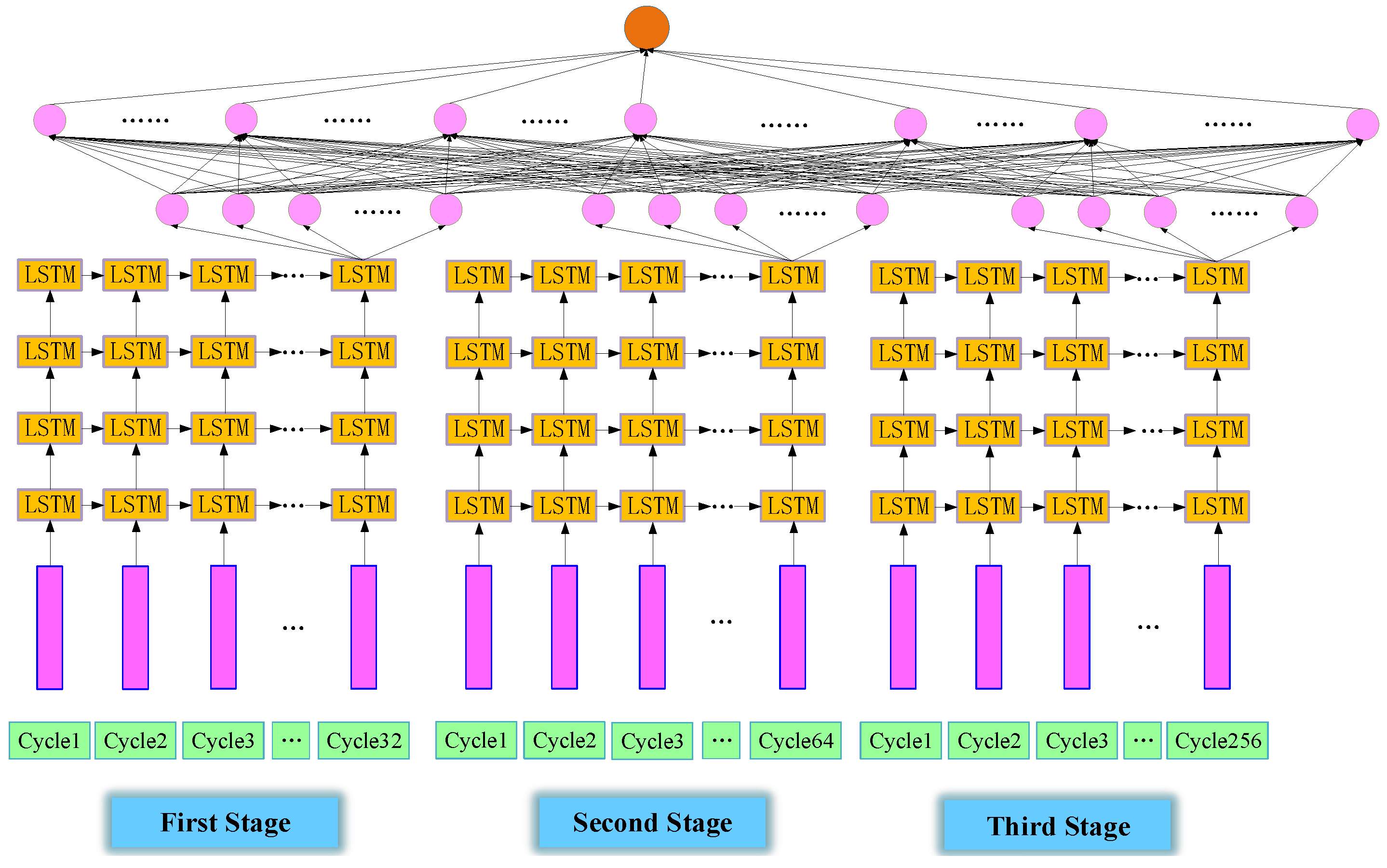
A method for solving the characteristics of pressure exertion based on historical data is proposed, and a three-step prediction model for pressure exertion is designed and discussed. In the first step, a deep spatiotemporal sequence model is selected for support resistance prediction. In the second step, an image segmentation-based classification model is chosen for pressure label classification. In the third step, a fusion model consisting of three LSTM networks is designed.

(3)

The model was trained using data from 10 working faces in the Datong mining area. The training set error for the first step was 1.83 kN, and the test set error was 4.65 kN. The training set accuracy for the second step was 99.38%, and the test set accuracy was 97.77%. For the third step, the dynamic pressure coefficient error was 0.17, the maximum resistance error during pressure exertion was 810.93 kN, the error in the number of cycles during pressure exertion was 9.96 cycles, and the accuracy for pressure exertion type classification was 92.35%.

(4)

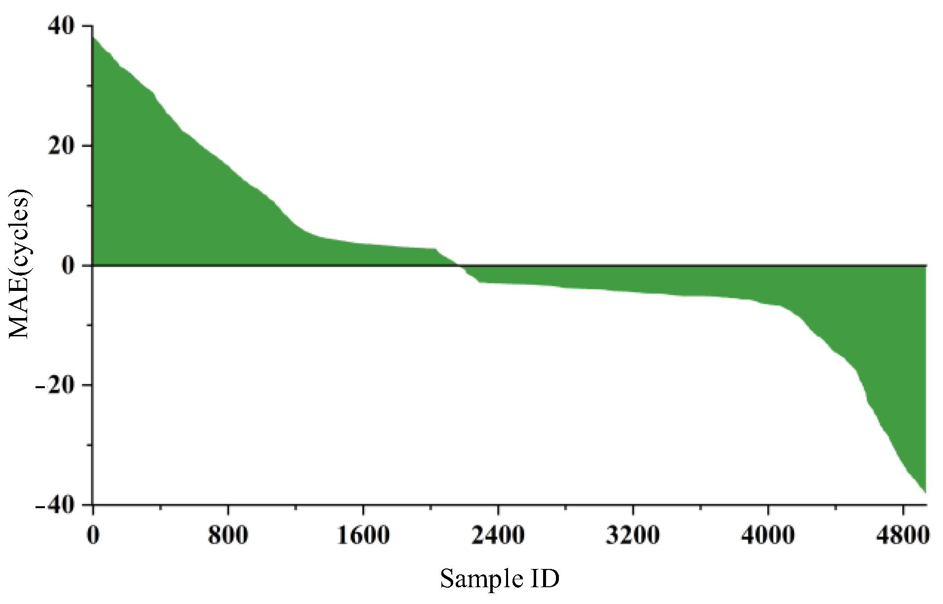
To simulate the actual conditions of application scenarios, the input data for the second and third steps were set as the output data from the previous step, and the model was evaluated. The model’s mean absolute error for support resistance prediction was 1035.21 kN, and its classification accuracy for coordinate unit pressure labels was 82.90%, with a cycle pressure label accuracy of 90.93%. In the simulated scenario, there were 9922 actual instances of pressure exertion, and the model predicted 10336 instances, with 9046 of these predictions corresponding to actual instances of pressure exertion. An evaluation was conducted of the feature parameter predictions for 4946 instances of pressure exertion that included three complete pressure exertion phases. The mean absolute error for the dynamic pressure coefficient was 0.21, the maximum resistance during pressure exertion was 1218.31 kN, the number of cycles during pressure exertion was 11.03 cycles, and the classification accuracy for pressure exertion types was 91.75%.

References

1. Wang, S.; Shen, Y.; Song, S.; Liu, L.; Gu, L.; Wei, J. Change of coal energy status and green and low-carbon development under the “dual carbon” goal. J. China Coal Soc. 2023, 48, 2599–2612. (In Chinese) [Google Scholar] [CrossRef]
2. Wu, Q.; Tu, K.; Zeng, Y.F.; Liu, S.Q. Discussion on the main problems and countermeasures for building an upgrade version of main energy (coal) industry in China. J. China Coal Soc. 2019, 44, 1625–1636. (In Chinese) [Google Scholar] [CrossRef]
3. Wang, X.; Xu, L.; Gao, Q.; Liu, N.; Wang, C.; Li, K. Effect of consumer subsidies on coal mine efficiency and its transmission mechanism. Energy Policy 2024, 196, 114412. [Google Scholar] [CrossRef]
4. Zhao, Y.; Zhang, Z.; Jia, T. Analysis of Coal Mine Safety Accidents and Research on Safety Countermeasures in China from 2010 to 2021. Coal Technol. 2023, 42, 128–131. (In Chinese) [Google Scholar] [CrossRef]
5. Fan, C.; Wang, Y.; Yang, L.; Xu, S.; Qiu, F. Statistics and Regularity Analysis of Coal Mine Safety Accidents from 2012 to 2021. Min. Res. Dev. 2023, 43, 182–188. (In Chinese) [Google Scholar] [CrossRef]
6. Zhang, C.; Wang, B.; Su, M. Study on Law of Coal Mine Accidents in Shanxi Province from 2016 to 2022. Coal Technol. 2023, 42, 187–190. (In Chinese) [Google Scholar] [CrossRef]
7. Cai, G.S.; An, L.Q.; Zhu, X.X.; An, J.L.; Mao, L.T. Study on Close Coal Seam Pressure Behavior Law of Zhong Xing Mine by Physical Model. Appl. Mech. Mater. 2012, 204, 1439–1444. [Google Scholar] [CrossRef]
8. Li, X.; Liu, Y.; Ren, X.; Wu, X.; Zhou, C. Roof breaking characteristics and mining pressure appearance laws in close distance coal seams. Energy Explor. Exploit. 2023, 41, 728–744. [Google Scholar] [CrossRef]
9. Wang, J.; Zhang, Q.; Zhang, J.; Yin, W.; Wang, Y.; Zhang, Q. Technical system and mining pressure law of full mining and local filling in a deep mine. Int. J. Oil Gas Coal Technol. 2023, 33, 369–387. [Google Scholar] [CrossRef]
10. Zhou, Z.; Huang, Y.; Zhao, C. Distribution Law of Mine Ground Pressure via a Microseismic Sensor System. Minerals 2023, 13, 649. [Google Scholar] [CrossRef]
11. Lan, T.; Liu, Y.; Yuan, Y.; Liu, H.; Liu, H.; Zhang, S.; Wang, S. Mine pressure behavior law of isolated island working face under extremely close goaf in shallow coal seam. Sci. Rep. 2023, 13, 20576. [Google Scholar] [CrossRef] [PubMed]
12. Wang, Y.; Zhang, Y.; Xue, B.; Li, J.; Han, L.; Yu, H. Research on mine pressure law of isolated working face in close-distance thin coal seam under the influence of remaining coal pillar. Int. J. Oil Gas Coal Technol. 2024, 35, 299–320. [Google Scholar] [CrossRef]
13. Wu, Z.; Sun, Q.; Wang, Y. Evolution Laws of Water-Flowing Fracture Zone and Mine Pressure in Mining Shallow-Buried, Hard, and Extra-Thick Coal Seams. Appl. Sci. 2024, 14, 2915. [Google Scholar] [CrossRef]
14. Jia, C.; Lai, X.; Cui, F.; Xu, H.; Zhang, S.; Li, Y.; Zong, C.; Luo, Z. Mining Pressure Distribution Law and Disaster Prevention of Isolated Island Working Face Under the Condition of Hard “Umbrella Arch”. Rock Mech. Rock Eng. 2024, 57, 8323–8341. [Google Scholar] [CrossRef]
15. Fu, Y.; Chen, L.; Xiong, H.; Chen, X.; Lu, A.; Zeng, Y.; Wang, B. Data-driven real-time prediction for attitude and position of super-large diameter shield using a hybrid deep learning approach. Undergr. Space 2024, 15, 275–297. [Google Scholar] [CrossRef]
16. Jing, Y.; Bian, Y.; Hu, Z.; Wang, L.; Xie, X.Q.S. Deep Learning for Drug Design: An Artificial Intelligence Paradigm for Drug Discovery in the Big Data Era. AAPS J. 2018, 20, 58. [Google Scholar] [CrossRef]
17. Guo, S.; Agarwal, M.; Cooper, C.; Tian, Q.; Gao, R.X.; Grace, W.G.; Guo, Y.B. Machine learning for metal additive manufacturing: Towards a physics-informed data-driven paradigm. J. Manuf. Syst. 2022, 62, 145–163. [Google Scholar] [CrossRef]
18. Cai, S.; Fang, F.; Tang, X.; Zhu, J.; Wang, Y. A Hybrid Data-Driven and Data Assimilation Method for Spatiotemporal Forecasting: PM2.5 Forecasting in China. J. Adv. Model. Earth Syst. 2024, 16, e2023MS003789. [Google Scholar] [CrossRef]
19. Dariane, A.B.; Behbahani, M.R.M. Maximum energy entropy: A novel signal preprocessing approach for data-driven monthly streamflow forecasting. Ecol. Inform. 2024, 79, 102452. [Google Scholar] [CrossRef]
20. Wang, H.; Li, B.; Gong, J.; Xuan, F.Z. Machine learning-based fatigue life prediction of metal materials: Perspectives of physics-informed and data-driven hybrid methods. Eng. Fract. Mech. 2023, 284, 109242. [Google Scholar] [CrossRef]
21. Xiao, T.; Zhang, L.M. Data-driven landslide forecasting: Methods, data completeness, and real-time warning. Eng. Geol. 2023, 317, 107068. [Google Scholar] [CrossRef]
22. Chen, Y.Q.; Liu, C.Y.; Liu, J.R.; Yang, P.J.; Lu, S.; Wei, J.K. Study on support pressure continuity classification and mine pressure characteristics by unifying spatiotemporal characteristics modelling. J. Min. Saf. Eng. 2021, 38, 1–11. (In Chinese) [Google Scholar] [CrossRef]
23. Zhao, Y.X.; Yang, Z.L.; Ma, B.J.; Song, H.H.; Yang, D.H. Deep learning prediction and model generalization of ground pressure for deep longwall face with large mining height. J. China Coal Soc. 2020, 45, 54–65. (In Chinese) [Google Scholar] [CrossRef]
24. Yang, Z. Separation and Extraction of Measured Time Series Data and Advanced Prediction of Mineral Pressure. Master’s Thesis, Taiyuan University of Technology, Taiyuan, China, 2022. (In Chinese). [Google Scholar]
25. Liu, Y. Mineral Pressure Manifestation Prediction Method Based on Machine Learning. Master’s Thesis, Xi’an University of Science and Technology, Xi’an, China, 2021. (In Chinese). [Google Scholar]
26. Miao, Y. Research on Prediction of Working Face Periodic Pressure Based on Recurrent Neural Network. Master’s Thesis, Xi’an University of Science and Technology, Xi’an, China, 2021. (In Chinese). [Google Scholar]
27. Li, Z. Research on Prediction Method of Mining Pressure in Coal Face Based on LSTM. Master’s Thesis, Xi’an University of Science and Technology, Xi’an, China, 2020. (In Chinese). [Google Scholar]
28. Gao, X.; Hu, Y.; Liu, S.; Yin, J.; Fan, K.; Yi, L. An AGCRN Algorithm for Pressure Prediction in an Ultra-Long Mining Face in a Medium-Thick Coal Seam in the Northern Shaanxi Area, China. Appl. Sci. 2023, 13, 11369. [Google Scholar] [CrossRef]
29. He, K.; Zhang, X.; Ren, S.; Sun, J. Deep Residual Learning for Image Recognition. In Proceedings of the 2016 IEEE Conference on Computer Vision and Pattern Recognition (CVPR), Las Vegas, NV, USA, 27–30 June 2016; pp. 770–778. [Google Scholar] [CrossRef]
30. Szegedy, C.; Liu, W.; Jia, Y.; Sermanet, P.; Reed, S.; Anguelov, D.; Erhan, D.; Vanhoucke, V.; Rabinovich, A. Going Deeper with Convolutions. In Proceedings of the 2015 IEEE Conference on Computer Vision and Pattern Recognition (CVPR), Boston, MA, USA, 7–12 June 2015; pp. 1–9. [Google Scholar] [CrossRef]
31. Simonyan, K.; Zisserman, A. Very Deep Convolutional Networks for Large-Scale Image Recognition. arXiv 2014. [Google Scholar] [CrossRef]
32. Sutskever, I.; Vinyals, O.; Le, Q.V. Sequence to Sequence Learning with Neural Networks. arXiv 2014. [Google Scholar] [CrossRef]
33. Chen, Y.; Liu, C.; Liu, J.; Yang, P.; Wu, F.; Liu, S.; Liu, H.; Yu, X. Intelligent prediction for support resistance in working faces of coal mine: A research based on deep spatiotemporal sequence models. Expert Syst. Appl. 2024, 238, 122020. [Google Scholar] [CrossRef]
34. Wang, Y.; Long, M.; Wang, J.; Gao, Z.; Yu, P.S. PredRNN: Recurrent Neural Networks for Predictive Learning using Spatiotemporal LSTMs. In Proceedings of the 31st Conference on Neural Information Processing Systems (NIPS 2017), Long Beach, CA, USA, 4–9 December 2017. [Google Scholar]
35. Krizhevsky, A.; Sutskever, I.; Hinton, G.E. ImageNet Classification with Deep Convolutional Neural Networks. Commun. ACM 2017, 60, 84–90. [Google Scholar] [CrossRef]
36. Hariharan, B.; Arbeláez, P.; Girshick, R.; Malik, J. Simultaneous Detection and Segmentation. In Proceedings of the 13th European Conference on Computer Vision (ECCV), Zurich, Switzerland, 6–12 September 2014; Volume 8695, pp. 297–312. [Google Scholar] [CrossRef]
37. Gupta, S.; Girshick, R.; Arbeláez, P.; Malik, J. Learning Rich Features from RGB-D Images for Object Detection and Segmentation. In Proceedings of the 13th European Conference on Computer Vision (ECCV), Zurich, Switzerland, 6–12 September 2014; Volume 8695, pp. 345–360. [Google Scholar] [CrossRef]
Figure 1. Schematic diagram of the grid model for the entire working face area.
Applsci 15 04192 g001
Figure 2. Real-time classification model for pressure labels based on image classification.
Applsci 15 04192 g002
Figure 3. Real-time classification model for pressure labels based on image segmentation.
Applsci 15 04192 g003
Figure 4. Schematic diagram of pressure label distribution curves for different cycles.
Applsci 15 04192 g004
Figure 5. Prediction model for pressure exertion characteristic parameters.
Applsci 15 04192 g005
Figure 6. Distribution of working faces for data acquisition.
Applsci 15 04192 g006
Figure 7. Heatmap of support resistance data distribution in part of the mining area of LW8102.
Applsci 15 04192 g007
Figure 8. Heatmap of support resistance data distribution across nine data collection working faces.
Applsci 15 04192 g008
Figure 9. Training process curve of the support resistance prediction model.
Applsci 15 04192 g009
Figure 10. Training process curve of the pressure label classification model based on image classification.
Applsci 15 04192 g010
Figure 11. Training process curve of the pressure label classification model based on image segmentation.
Applsci 15 04192 g011
Figure 12. Curve of the support resistance prediction error varying with the prediction sequence length.
Applsci 15 04192 g012
Figure 13. Distribution of prediction errors for dynamic pressure coefficients across all samples.
Applsci 15 04192 g013
Figure 14. Distribution of prediction errors for the maximum resistance during pressure exertion across all samples.
Applsci 15 04192 g014
Figure 15. Distribution of prediction errors for the number of cycles during pressure exertion across all samples.
Applsci 15 04192 g015