Abstract
To consider the influence of material parameter uncertainty on the structural deformation of a dam effectively and to establish a reasonable and reliable safety monitoring index for the displacement of a rockfill dam, a method for determining the displacement monitoring index of a rockfill dam based on stochastic finite element analysis is proposed in this paper. Firstly, uncertainty in the mechanical parameters of the rockfill material is simulated via the correlation log-normal random field, and the statistical characteristics of the dam displacement under the stability of the resultant distribution are obtained through several structural analyses, thus constructing a stochastic finite element method-based monitoring model (SFEMM model); subsequently, the boundary values of the water pressure component are determined based on the statistical characteristics of the displacement at different water levels, and the displacement monitoring index is determined by inputting it into the SFEMM model. Finally, the index is applied to the actual panel rockfill dam project. Finally, the method is applied to the actual concrete-face rockfill dam project. The results show that the SFEMM model achieves higher prediction accuracy and stability than other monitoring models, with the relative error lower than 4.7% and the correlation coefficient higher than 0.96, and the monitoring index is accurate and reasonable. This method provides a scientific and reliable new idea for the safety monitoring of rockfill dams.
1. Introduction
To promote the benign development of the global ecological environment, governments have made great efforts to develop clean energy. In this context, pumped storage projects, as one of the most mature energy storage methods, have been rapidly developed and constructed. Rockfill dams are extensively utilized in the context of pumped storage projects, primarily due to their cost-effectiveness and high structural reliability. As the construction of rockfill dams accelerates and their height increases, the accurate monitoring of their structural changes and the reasonable determination of safety monitoring indices becomes increasingly imperative. This is essential for ensuring the safe operation of these dams [1,2].
The purpose of determining the monitoring index is to assess and predict the dam’s ability to resist possible loads and thus to determine the extreme value (maximum allowable value) and warning value (a certain percentage of extreme value) of the effector under that load combination. The prevailing methods for determining the monitoring index of dam displacement are the confidence interval method [3], the typical small probability method [4], and the structural analysis method [5]. The former two are mathematical statistics methods that utilize probability statistics theory and existing monitoring data to assess the monitoring displacements of dams. They offer the advantage of being simple and easy to operate. However, in dam displacement, monitoring data are less extensive and are not obtained through the most unfavorable loading conditions; the monitoring indexes determined through the two methods do not depict the extreme value of the real state. In addition, the physical concepts of the monitoring indexes based on mathematical and statistical methods are not clear because they are not related to the mechanical characteristics and deformation mechanisms of the dam structure. The structural analysis method adopts the finite unit method to establish a model to simulate the force characteristics of the dam, and the physical concept is clear, so it can calculate the deformation and stress change of the dam body under various working conditions and then simulate certain loading conditions that have never been encountered, which is more suitable for determining the monitoring index of the safety of the whole life cycle of the dam [6,7,8,9].
In the conventional monitoring index determination based on the structural analysis method, it is generally accepted that the mechanical parameters of the rockfill material are determined. That is to say that the parameters of the laboratory geotechnical test are used for the structural calculations and, consequently, for the determination of the water pressure component [10]. However, in actual project implementation, influenced by factors such as geological investigation, geotechnical test, design assumptions, construction technology, and construction conditions, significant variations in the rockfill materials are evident. These variations encompass the physical properties of the rockfill materials (density, pore ratio, average particle size, etc.) and mechanical parameters. The existence of certain uncertainties and random distribution characteristics has been demonstrated in the extant references [11,12,13]. Ignoring these uncertainties in safety monitoring and risk evaluation has been shown to have a serious impact on the deformation prediction and safety analysis of dams, as shown in Table 1, resulting in monitoring index deviation and difficulties in accurately and comprehensively responding to the true operational state of a rockfill dam [14,15,16].

Table 1.
The impact of not considering uncertainty on the analysis of dam structures.
To fully consider the impact of the uncertainty of the above parameters on the deformation of the rockfill dam, simulate the displacement changes of the dam body more realistically, and establish reasonable and accurate displacement monitoring indexes for the rockfill dam through structural analysis, this paper proposes a new method for formulating monitoring indexes. The proposed method adopts Gaussian random field simulation to model uncertainty due to the rockfill material, building the water pressure component using stochastic finite element method (SFEM) in order to establish a hybrid monitoring model of rockfill displacement. The hybrid monitoring model is then used to predict the trend in the dam displacement and substitute the water pressure component under a confidence interval to form the limit of displacement fluctuation interval as the monitoring index of rockfill dam displacement, as show in Figure 1. Finally, the advancement and reasonableness of the displacement monitoring index are verified by taking the actual project monitoring data as an example.
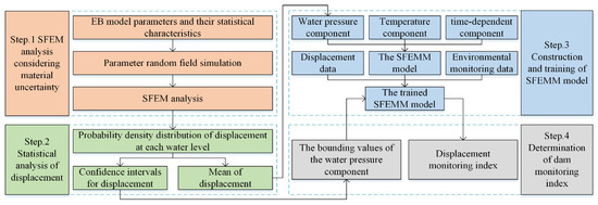
Figure 1.
Steps for determining displacement monitoring index for rockfill dam considering material uncertainty.
2. Methodology
2.1. SFEM-Based Simulation Method for Parametric Uncertainty
2.1.1. Standard Gaussian Random Fields
To realize the analysis of the uncertainty of geotechnical materials, scholars have incorporated random field theory into the numerical computational analysis of finite elements and established the stochastic finite element method to simulate the parameter uncertainty and correlation of geotechnical materials in the spatial range. The degree of correlation of a geotechnical parameter between two points in space is usually expressed by the autocorrelation coefficient, ρ, which is a function of the distance between the two points [21]:
where are the eigenvalues of the grid parameter distributions of the random field cell with center-point coordinates , respectively; COV(·) is the covariance of the grid parameter distributions, and Var(·) is the variance of the grid parameter distributions.
In accordance with the random field model of soil advanced by Lumb [8], it is possible to adopt a discretization method for random fields, such as the so-called center-point method and level expansion method [21,22]. Among these methods, the center-point method based on Cholesky decomposition has been demonstrated to exhibit high computational efficiency, as well as adaptive adaptability in comparison to competing approaches [23]. In this paper, therefore, the focus is on the use of the center-point method of Cholesky decomposition for the simulation of random fields. The random field is defined by parameters including the mean, variance, correlation, and correlation distance of the variables. It is generally assumed that the mean and variance are independent of the spatial location of the random field, and the correlation is only related to the relative distance between two points in space [24]. In practical engineering applications, due to the scarcity of measured data, the use of theoretical correlation functions, such as the Gaussian correlation function, is predominantly employed to represent the autocorrelation of the same parameter in geotechnical materials [25]:
where is the horizontal relative distance, , is the vertical relative distance, , is the horizontal relative distance, , and are the fluctuation ranges in three directions. In addition to autocorrelation, there are also cross-correlations between different parameters in geotechnical materials, which can also be expressed by correlation functions, i.e., the autocorrelation coefficients matrix and correlation coefficients matrix can be obtained via correlation function modeling.
2.1.2. Correlated Log-Normal Random Fields for Geotechnical Materials
In the context of geotechnical materials, it is observed that the majority of mechanical parameters adhere to a lognormal distribution [26,27,28]. Consequently, the autocorrelation coefficient matrix and the cross-correlation coefficient matrix of the aforementioned standard Gaussian random field must undergo a change through the Nataf transformation. This ensures that the representation of the autocorrelation and cross-correlation between the geotechnical material parameters in the lognormal random field is accurately captured [29]. It is imperative to note that, during the process of random field transformation, a decomposition of the correlation coefficient matrix in the standard normal space becomes essential. This non-linear transformation process entails a modification in the correlation coefficients between parameters across different spaces. Consequently, the equivalent correlation coefficients in the standard normal space must be calculated [30]:
where is the autocorrelation coefficient of the original random variable, is the equivalent autocorrelation coefficient of the standard normal random variable, is the equivalent cross-correlation coefficient of the standard normal random variable, is the cross-correlation coefficient of the original random variable, and are the simulated values of the unit parameter Gaussian random field with the centroid coordinates and , respectively, is the two-dimensional joint probability density function for the cross-correlation coefficient , and is the autocorrelation correction coefficient, which can be set to a value of 1 because the difference between the equivalent autocorrelation coefficient and the original autocorrelation coefficient has a small and negligible effect on the calculation results [31].
After calculating the above standard normal spatial equivalent correlation coefficients, the equivalent cross-correlation coefficient matrix and autocorrelation coefficient matrix can be obtained, respectively. Subsequently, Cholesky decomposition is applied to them, e.g., and , to obtain the lower triangular matrices L1 and L2. The independent standard normal random sample matrix ξ of the soil parameters is established and multiplied by the two lower triangular matrices, respectively. The associated standard Gaussian random field can be obtained [32]:
where is the associated standard normal random sample matrix.
The associated log-normal random field can be obtained by taking the associated standard Gaussian random field to be exponential through the equal probability transformation method:
where is the standard deviation of the normal variable , , is the mean of the normal variable , , is the standard deviation of the log-normal variable , and is the mean of the log-normal variable .
Cholesky decomposition is performed on the equivalent cross-correlation coefficient matrix and equivalent autocorrelation coefficient matrix, respectively, to obtain the correlated log-normal random field in three-dimensional space. To facilitate the simulation and analysis, the random field adopts the same mesh distribution as the finite element model; i.e., the random field elements have the same size and number as the finite element mesh [33]. The SFEM represents a non-invasive methodology that exhibits significant practical advantages in comparison with conventional invasive methods such as the perturbation stochastic finite element method and the spectral stochastic finite element method. A key advantage of the SFEM lies in its ability to circumvent the necessity for modification of the finite element source code whilst eliminating the coupling between finite element analysis and probabilistic analysis [34].
2.2. Determination of Displacement Monitoring Index for Rockfill Dams
2.2.1. Hybrid Monitoring Model
The hybrid monitoring model for rockfill dam displacement can be defined as a regression model that represents the nonlinear relationship between dam displacement and environmental variables [10,35,36].
where δ is the displacement of the dam body; , , and represent the displacement components in the three directions of the dam body, respectively, is the water pressure component, which is determined by the expression of the water level–displacement relationship obtained from structural calculations and can generally be determined via polynomial curve fitting, as shown in Equation (7), is the temperature component, and is the time-dependent component. The temperature component and the time-dependent component are calculated using the expressions in the statistical model [10], as shown in Equations (8) and (9).
where H is the upstream water depth, is the average temperature of i days before the observation day, and, when i = 0, it means the temperature on the day of observation, t is the time (days) counted from a certain day, m is the number of polynomial terms, and it is generally taken as 3~4, m1 and m2 are the number of temperature factors and cycles, and they are generally taken as 9~10, θ is the time-dependent factor, θ = t/100, and a, b, and c are coefficients to be determined.
In the context of the engineering safety monitoring process, a range of factors contribute to discrepancies between the activation time of the instrument and the initial displacement values recorded for the dam. These discrepancies can be attributed to the failure and replacement of monitoring equipment, variations in natural or human-made factors, and the inherent variability associated with the measurement process. Consequently, it becomes essential to implement a correction parameter, designated as L, to the water pressure component to ensure the accuracy of the data. The expression of the hybrid monitoring model is thus modified as follows [37]:
In order to establish the hybrid model under discussion, it is first necessary to employ the stochastic finite element method to calculate the displacement of the dam body in question under differing water levels. This calculation is then fitted to form the water pressure component, thus taking into account the effect of uncertainties pertaining to the physical and mechanical parameters of the rockfill in question. The primary structure of the rockfill dam comprises the following components: upstream, main, and secondary rockfill, with the Duncan–Chang E-B model being utilized to describe its stress–strain relationship. Due to the variability in the material properties in different rockfill zones, the random field eigenvalues of the parameters are not identical, thus necessitating the execution of random field parameter simulations according to the material partition, and subsequently assigning the stochastic results to each element for FEM analysis. The computational demands of conducting random field simulations for all parameters in the model to establish the water pressure component via SFEM can be prohibitive, particularly given the varied impact of each parameter on rockfill deformation in the E-B model. Previous research has indicated that the parameters Kb, φ0, and n in the E-B model have a significant influence on dam displacement when compared to other model elements [38,39,40,41]. Consequently, to enhance the efficacy of the analysis, this study focuses on the random field simulation of the parameters Kb, φ0, and n in each rockfill zone of the dam. The remaining parameters are adopted from laboratory geotechnical tests.
The specific steps for constructing the water pressure component considering material uncertainty are as follows:
(1) The material parameters and their statistical eigenvalues for the random field simulation must be determined, and Latin hypercube sampling (LHS) must be used to generate an independent standard normal random sample matrix, X, of rockfill parameters by n times random sampling.
(2) For the upstream rockfill zone of the dam body, the Gaussian correlation function is selected, and the equivalent cross-correlation coefficient matrix and equivalent autocorrelation coefficient matrix in standard normal space are obtained using Equation (3). Subsequently, Cholesky decomposition is performed for its mapping in three directions, and the associated log-normal random field is obtained via Equations (4) and (5).
(3) Repeating steps (2) enables the simulation of the parameter random fields for the main and secondary rockfill zones of the dam, respectively. The random results are assigned to the corresponding finite element unit to obtain the parameter random field of the overall dam body.
(4) The dam measuring-point displacements of the above n-parameter random fields at different water levels are calculated via FEM. The displacement results are then subjected to statistical analysis, and the water pressure component is obtained by fitting the variation of the mean displacement at the measuring point with the reservoir level through Equation (7).
(5) Inputting the aforementioned water pressure component, in conjunction with the temperature component and the time-dependent component, into Equation (10) results in the construction of the stochastic finite element method-based monitoring model (SFEMM model) of the rockfill dam. The measured data from the pertinent dam measuring point are selected for partial least squares fitting, and the coefficients to be determined in each component are solved to obtain the trained SFEMM model of dam displacement.
In general, when the SFEMM model is evaluated, its computational accuracy is higher than that of traditional statistical models and conventional FEM models. When the accuracy of the SFEMM model is lower than that of conventional FEM models or traditional statistical models, it indicates that there is a significant deviation between the material parameters or random field parameters and the actual values. Experimental analysis can be conducted to further determine the parameter values. This issue should be analyzed specifically for practical engineering, and this paper does not delve into it in depth.
2.2.2. Displacement Monitoring Index
Utilizing the aforementioned stochastic finite element analysis, the results of the displacement calculation are then subjected to statistical organization, thereby yielding the probability density distribution of the dam’s displacement under each water level. Choosing the significance level α = 5% [12,42], the bounding values of the displacement confidence intervals at different water levels are calculated via Equation (11):
where μ and σ are the mean and standard deviation of the probability density distribution of the dam displacement under each water level, respectively; is the standardized fraction, which is 1.96 at the 5% significance level. Through the polynomial fitting of the boundary displacements y of the displacement confidence intervals at different water levels according to Equation (7), the interval boundary expressions for the water pressure component at a 5% significance level, i.e., the upper limit of the water pressure component and the lower limit of the water pressure component, are obtained. Subsequently, the upper and lower bound expressions of the water pressure component are substituted into the trained SFEMM model to obtain the displacement monitoring index of the rockfill dam.
In summary, a method for determining monitoring indexes for rockfill dams based on SFEM is proposed in this paper, taking into account material uncertainty. The proposed method is a refinement of the conventional confidence interval methods, utilizing the SFEM to simulate the water pressure component and thereby incorporating the uncertainty of the material parameters of the dam. This is in contrast to traditional structural analysis methods, which are unable to reflect the deformation mechanism of the dam body with the requisite realism and accuracy. The method’s ability to determine the relevant monitoring indices directly based on the monitoring model of the rockfill dam, even with limited data, is noteworthy. This approach, which integrates statistical characteristics of displacements under different water levels, demonstrates enhanced theoretical soundness and higher rationality through dynamic adjustments to monitoring indices in response to variations in the engineering environment.
3. Case Study
3.1. General Description of the Project
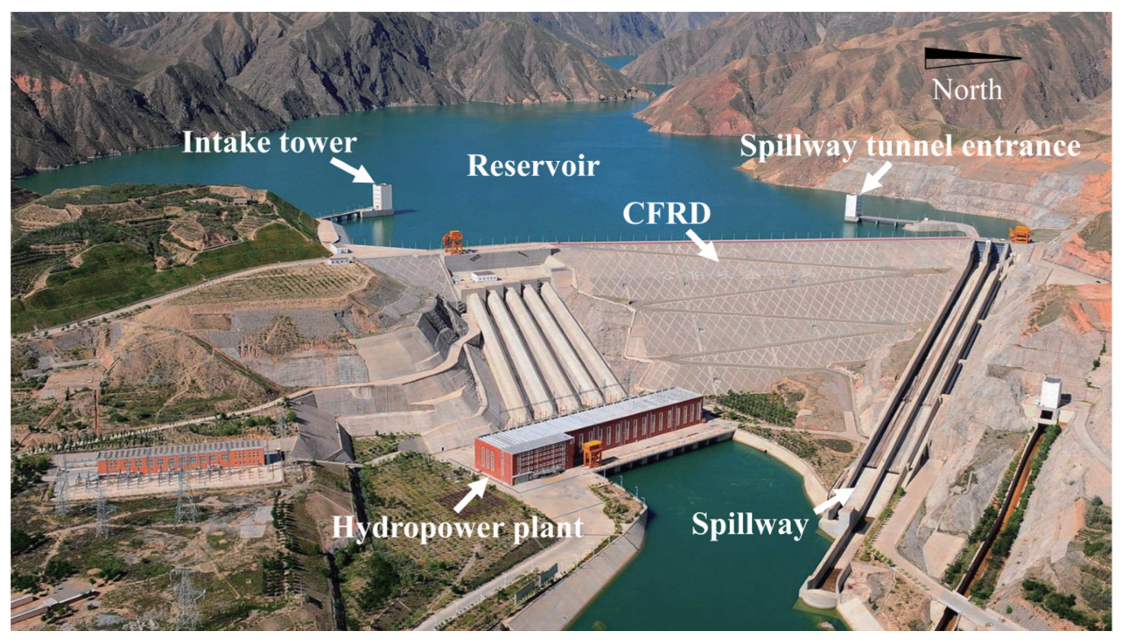
A water conservancy project is located in the upper reaches of the Yellow River in China, and the project’s primary structure is a concrete-face rockfill dam (CFRD). The dam maximum height (crest altitude–foundation altitude) is 132.20 m; the length and width of dam crest are 429.00 m and 10 m, respectively. The crest altitude is 2010.00 m, the altitudes of normal storage level and the design flood level are 2005.00 m, and the altitudes of calibration flood level and dead water level are 2008.28 m and 1975 m, respectively. The total storage capacity of the reservoir is 620 million cubic meters, with an average annual power generation of 5.14 billion kilowatt hours. The project layout is shown in Figure 2. The dam body is equipped with various monitoring programs such as displacement monitoring, seepage pressure monitoring, stress monitoring, etc. The location of the project and the dam surface displacement monitoring points are arranged as shown in Figure 3.

Figure 2.
Layout of engineering buildings.
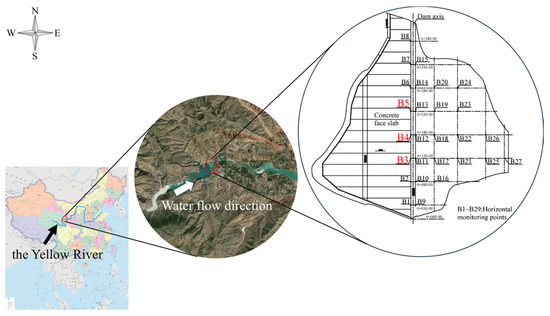
Figure 3.
Location of the project and layout of dam surface displacement monitoring.
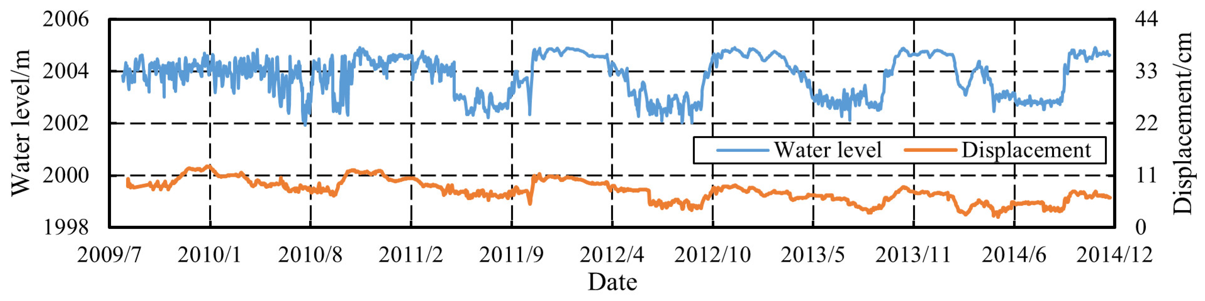
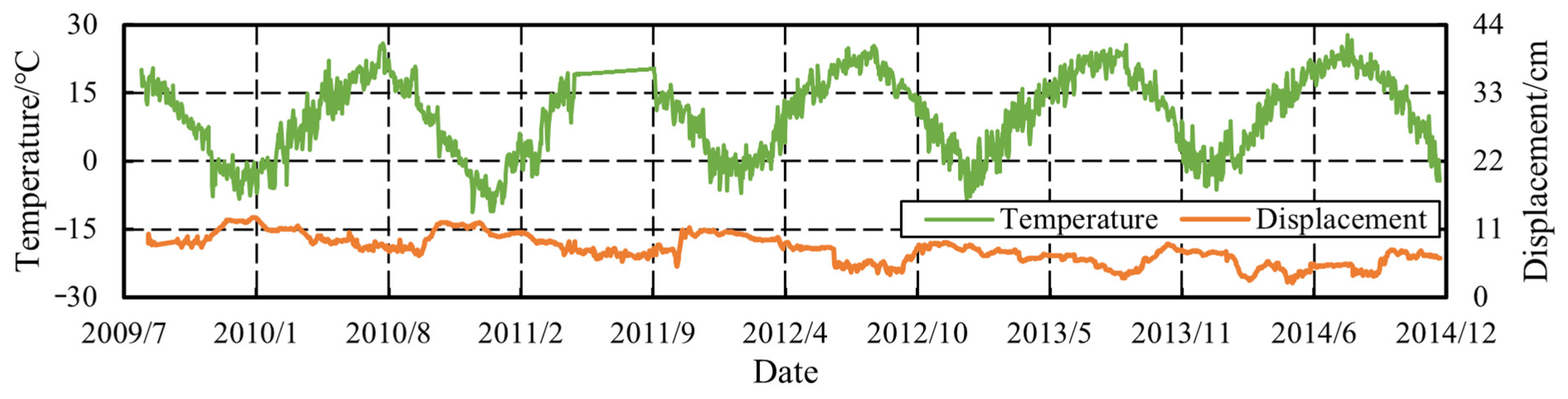
To verify the advancement and reasonableness of the index determination method, the displacement monitoring index is established by taking the horizontal displacement of measuring point B3, which is located at the top of the dam and close to the largest cross-section, as an example for analysis. The elevation of measuring point B3 is 2010.00 m, and the pile number is 0 + 130.00 m. The monitoring data pertaining to horizontal displacement at the designated measuring point were collected between August 2009 and December 2014, amounting to a total of 1760 sets. The hydrograph depicting the measured horizontal displacement of the measuring point, along with the upstream water level and ambient air temperature during the designated monitoring time period, is illustrated in Figure 4 and Figure 5, respectively.

Figure 4.
The horizontal displacement and the upstream water level.
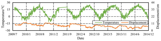
Figure 5.
The horizontal displacement and the air temperature.
Figures show that the horizontal displacement of B3 exhibits significant periodicity and a significant trend. Among them, there is a strong positive correlation between the displacement changes of the dam and the upstream reservoir water level, indicating that the periodic changes in the upstream reservoir water level are the main cause of the periodic displacement of the dam. The periodic variation of temperature also has a certain impact on the displacement of the dam. The trend displacement of the dam is mainly influenced by time, that is, the displacement changes with an increase in time.
3.2. The Methodological Description of the Analyzed Dam
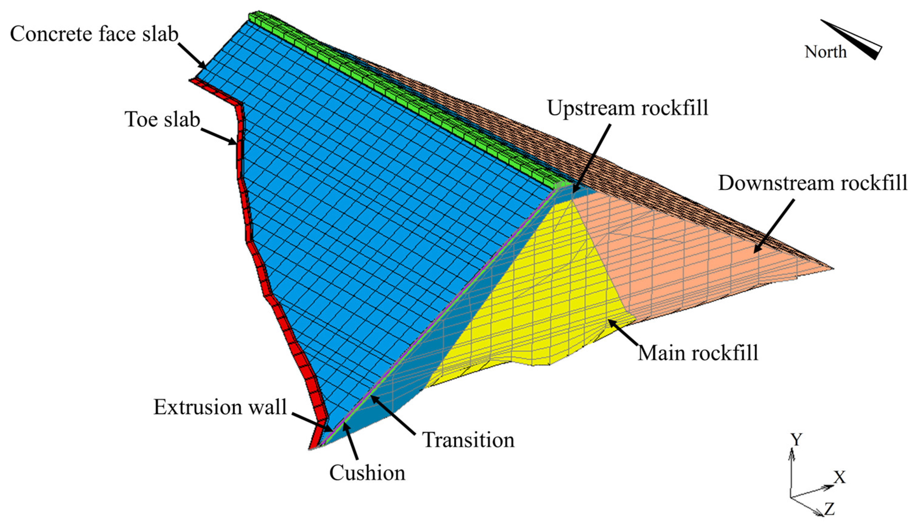
The three-dimensional finite element model of the rockfill dam is developed based on the specific geometry of the structure, with a focus on ensuring the integrity and accuracy of the model. The deformation of the dam foundation and its effects are not incorporated into the calculations due to the reliability of the bedrock at the dam foundation. CAE software is used for the finite-element mesh generation of the dam. The mesh size generally does not exceed 8% of the maximum dam height, according to references [40,41,43,44], and mesh refinement should be applied to some fine structures to ensure the mesh independence and analysis efficiency of the model calculation results. The finite element model comprises 10,378 nodes and 10,966 hexahedral eight-node isoparametric units. X is in the horizontal direction (positive towards downstream), Y is in the vertical direction (positive towards upstream), and Z is in the transverse direction (positive towards the right bank). To more realistically represent the actual construction and operation of the project, the normal storage level is utilized as an analytical condition and staged filling of the dam and staged water storage are simulated during calculation. Three-directional fixed constraints are implemented at the base of the dam, surface forces are applied to the upstream panel surface in order to simulate upstream reservoir pressure, and mass forces are applied to all elements of the model to simulate gravity. The dam body is segmented into material zones in accordance with the characteristics of the actual project, and the sequence from upstream to downstream comprises the following elements: concrete-face slab (toe slab), extrusion wall, cushion, transition, upstream rockfill, main rockfill, and downstream rockfill, as illustrated in Figure 6.

Figure 6.
Finite element modeling and material zones of rockfill dams.
In analyses using SFEM, the constitutive model of each material in the dam is selected as follows: (1) The face slab, extrusion wall, toe slab, and other concrete materials are simulated via a linear elasticity model. (2) The rockfill zone and cushion, transition, and other geotechnical materials are simulated using the Duncan E-B model. (3) The simulation of the concrete joints was undertaken by way of the connection element. The interface between concrete and geotechnical materials was modeled using the Goodman element. Due to the minimal impact of the connection element and the Goodman element on the internal displacement of the dam, the mechanical parameters were determined by referring to relevant references [45,46]; the mechanical parameters for the elements under consideration are set out in Table 2 and Table 3. Since the displacement of the dam originates principally from that of the rockfill materials [47,48], only the material mechanical parameters of the upstream rockfill, the main rockfill, and the downstream rockfill are simulated in this paper with random fields.
Table 2.
Material parameters of the connection element.
Table 3.
Material parameters of the Goodman element.
In the actual project, there are some differences in the physical and mechanical properties of the materials in each zone of the rockfill dam, but the overall variability is not significant, and there is no order of magnitude or multiplier difference in the values of parameters. In addition, the construction method, process, and steps of each zone are basically the same in the construction of rockfill dam, so the correlation distance of each zone should not differ too much. At present, there are relatively few studies on the correlation distance of the rockfill dam. According to the references [19,38,49,50], the horizontal correlation distance of the rockfill dam is generally set to 50–150 m, and the vertical correlation distance is generally 1/3~1/20 of the horizontal distance. The inverse analysis of the parameter of the rockfill dam in references [51,52,53,54] shows that the variation coefficient of the parameter of the main rockfill is less than 0.25, and that of the secondary rockfill is less than 0.35. Therefore, considering the material parameter characteristics and construction method and other factors, the relevant distance of 10 m (vertical direction) and 100 m (horizontal and transverse river direction) for the rockfill materials is adopted, and the coefficients of variation of material parameters of the upstream rockfill and the main rockfill are 0.1, and the coefficient of variation of material parameters of the downstream rockfill is 0.2. The parameters of each material of the rockfill dam are shown in Table 4, and the eigenvalues of the parameters random fields are shown in Table 5.
Table 4.
Values of material parameters for each zone.
Table 5.
Eigenvalues of the parameters random fields.
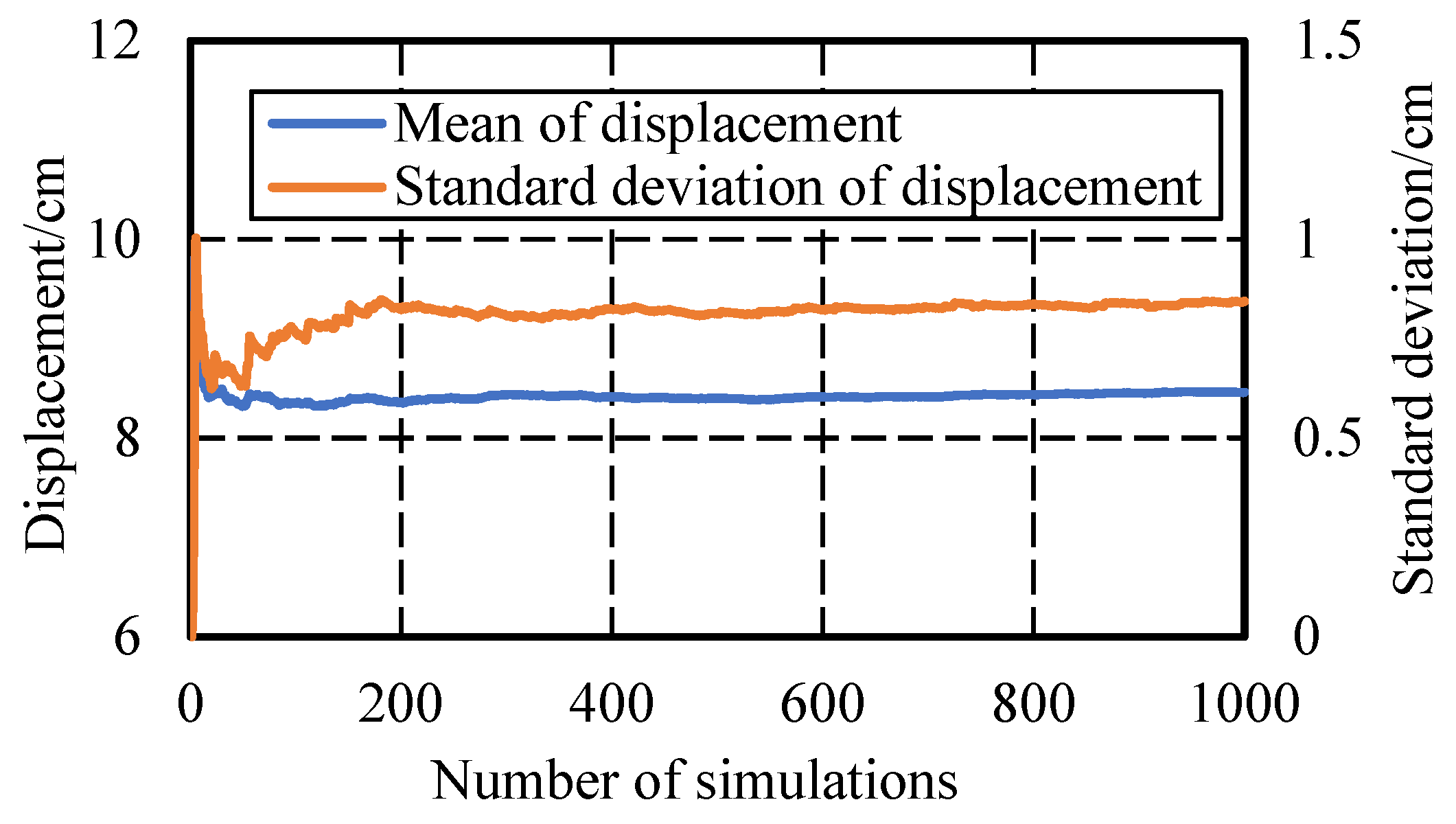
Based on the above material parameters and distribution characteristics, the sample matrix is generated via 1000-times random sampling using the LHS, and the equivalent cross-correlation coefficient matrix and autocorrelation coefficient matrix are calculated, respectively. The random field simulation method is subsequently implemented on the basis of Cholesky decomposition in order to simulate the mechanical parameters of the rockfill materials on 1000 occasions. It is observed that the random fields obey the log-normal distribution. The parameters in the random field are assigned to the elements, and then the probability density distribution of the displacement at the B3 measuring point under different water levels is obtained via SFEM calculation and statistical analysis. Since the results of stochastic finite element calculation show obvious uncertainty, the distribution characteristics of the results need to be verified smoothly. The calculation outcomes of the horizontal displacement of the designated B3 measurement point under a specified water level are tabulated, alongside the alterations in mean and standard deviation with respect to the number of random field simulations (Figure 7). The figure demonstrates that, upon reaching 400 random simulations, the mean and standard deviation of the SFEM results essentially stabilize. This indicates that, when the number of random field simulations exceeds 400, the random finite element calculation results achieve good stability and representativeness. The displacement of the dam body has a stable distribution type and distribution parameters, and it does not change significantly with an increase in random field simulations. Therefore, this paper uses the first 400 SFEM calculation results to construct the water pressure component.

Figure 7.
Stability of SREM results.
3.3. Analysis Results
3.3.1. Construction of SFEMM Model
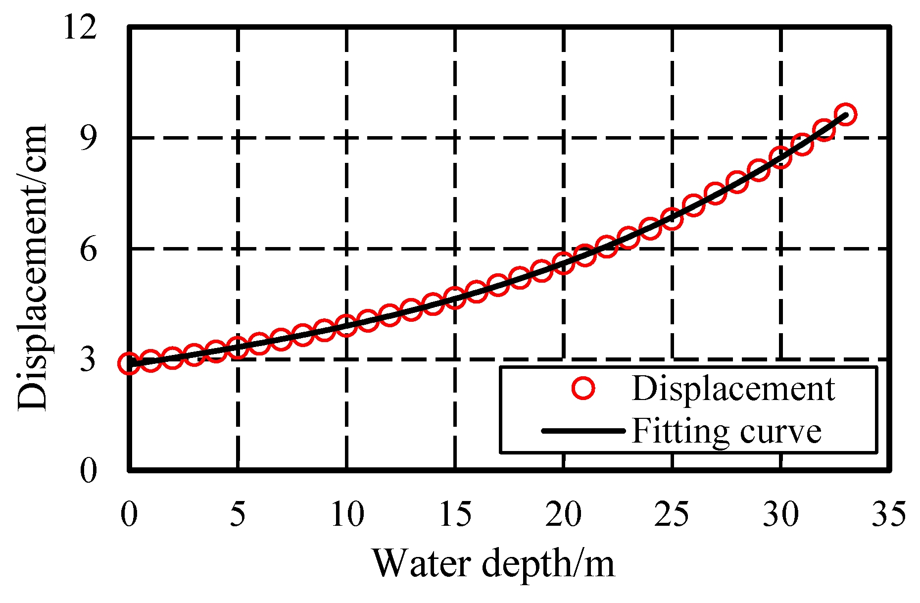
The findings from a series of 400 simulations employing the SFEM were subjected to rigorous analysis. The mean horizontal displacement at the B3 monitoring point was assessed under varying upstream water depths (the calculated water level minus the standard dead level). These data were then modeled through curve fittings, employing Equation (7), in order to ascertain the water pressure component expression. The efficacy of this approach is visualized in Figure 8, and the resulting fit can be expressed in Equation (12).

Figure 8.
Fitting curve of water pressure component.
Accordingly, the SFEMM model, taking into account the uncertainty of the rockfill, can be constructed:
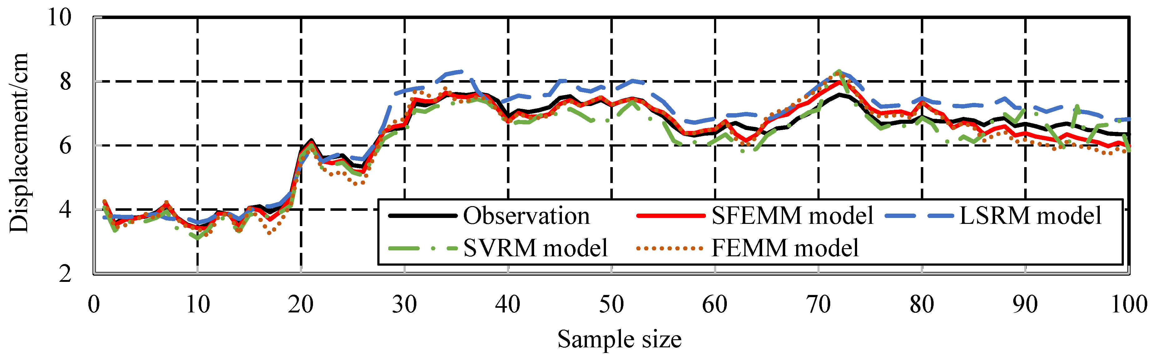
The established SFEMM model is utilized for the analysis and prediction of the measured horizontal displacement at monitoring point B3. A total of 1660 sets of monitoring data are employed for model training, and the final 100 sets are used for prediction analysis to evaluate the model’s accuracy. Furthermore, three additional monitoring models are selected for comparative prediction analysis to ascertain the superiority of the SFEMM model. These are the least squares regression monitoring model (LSRM model), the support vector machine monitoring model (SVRM model), and the conventional finite element method monitoring model (FEMM model). The results of this analysis are shown in Figure 9. (1) The prediction accuracy of each model for the first 28 sets of data is maintained at a high level, but with an increase in the number of prediction samples, the prediction error of each model shows a tendency to increase, and the prediction accuracy gradually decreases. (2) When the prediction data exceed 46 sets, the SVRM model is overfitted and exhibits poor stability, and its predicted values show the phenomenon of “oscillation”. (3) The prediction error of the LSRM model is obviously larger after 28 sets of data, and the prediction accuracy is lower. (4) It is evident that, while there is a strong correlation between prediction and measured values for both the FEMM and SFEMM models, the SFEMM model does in fact demonstrate a higher level of accuracy.

Figure 9.
Comparison of prediction results of various models.
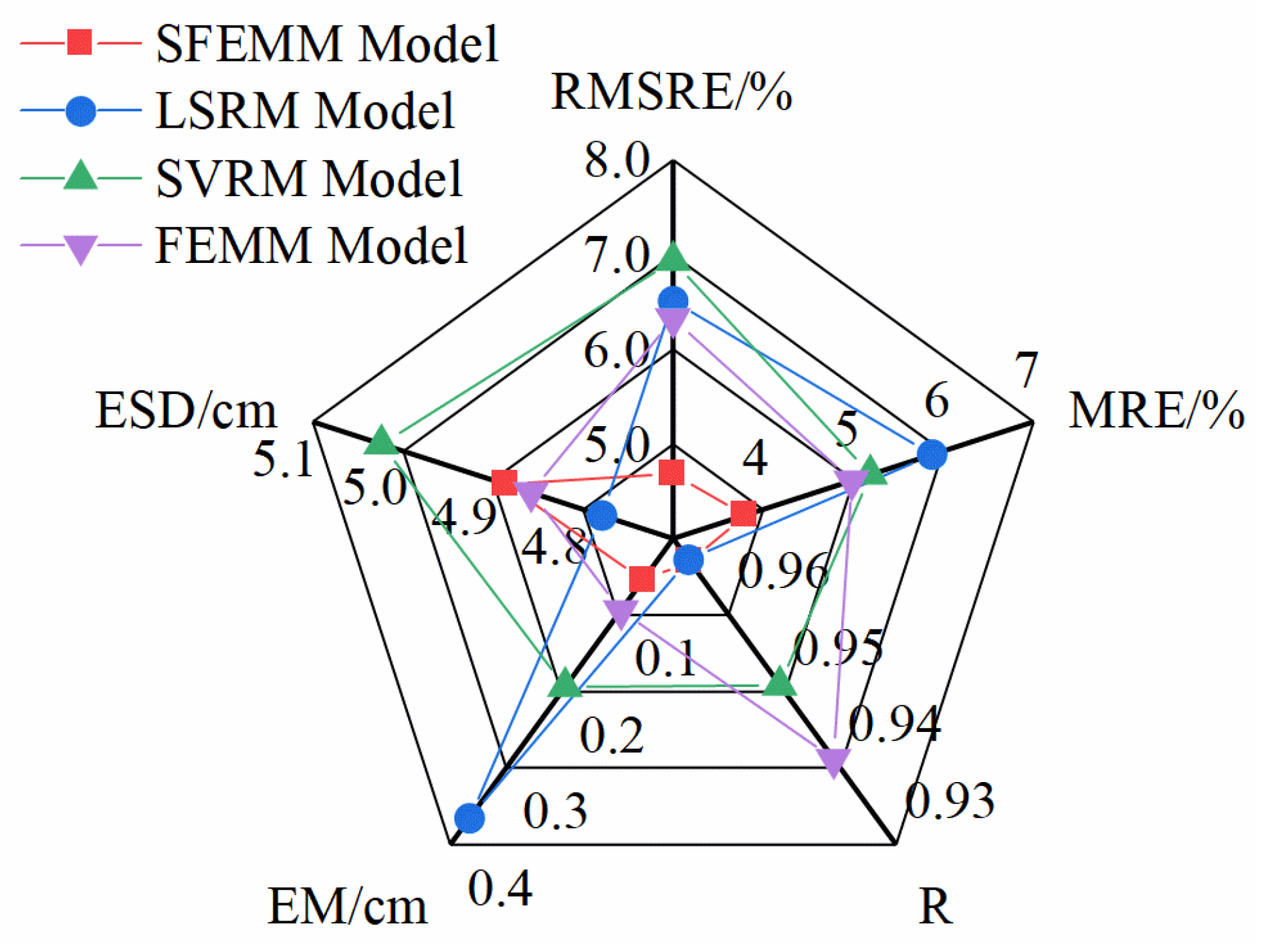
Additionally, the predictive performance of each model is evaluated using five indexes, as shown in Figure 10: (1) The SFEMM model has the smallest prediction errors among the four models, in which the RMSRE is less than 4.7%, and the MRE is less than 3.8%, whereas the other four models have the RMSRE greater than 6.3% cm, and the MRE is higher than 4.9%. (2) The correlation coefficients between the predicted and measured values from the SFEMM and LSRM models are all greater than 0.96, which is higher than those of the other monitoring models. (3) The distribution characteristics of the predicted values of the SFEMM model are closer to those of the measured values when the EM and ESD of the predicted and measured values of the models are compared.
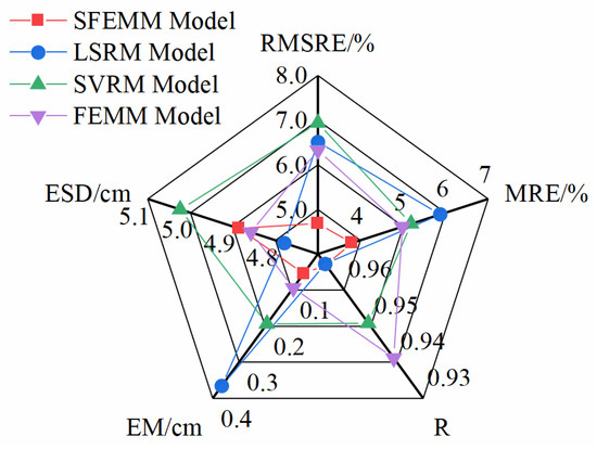
Figure 10.
Prediction error statistics for each model.
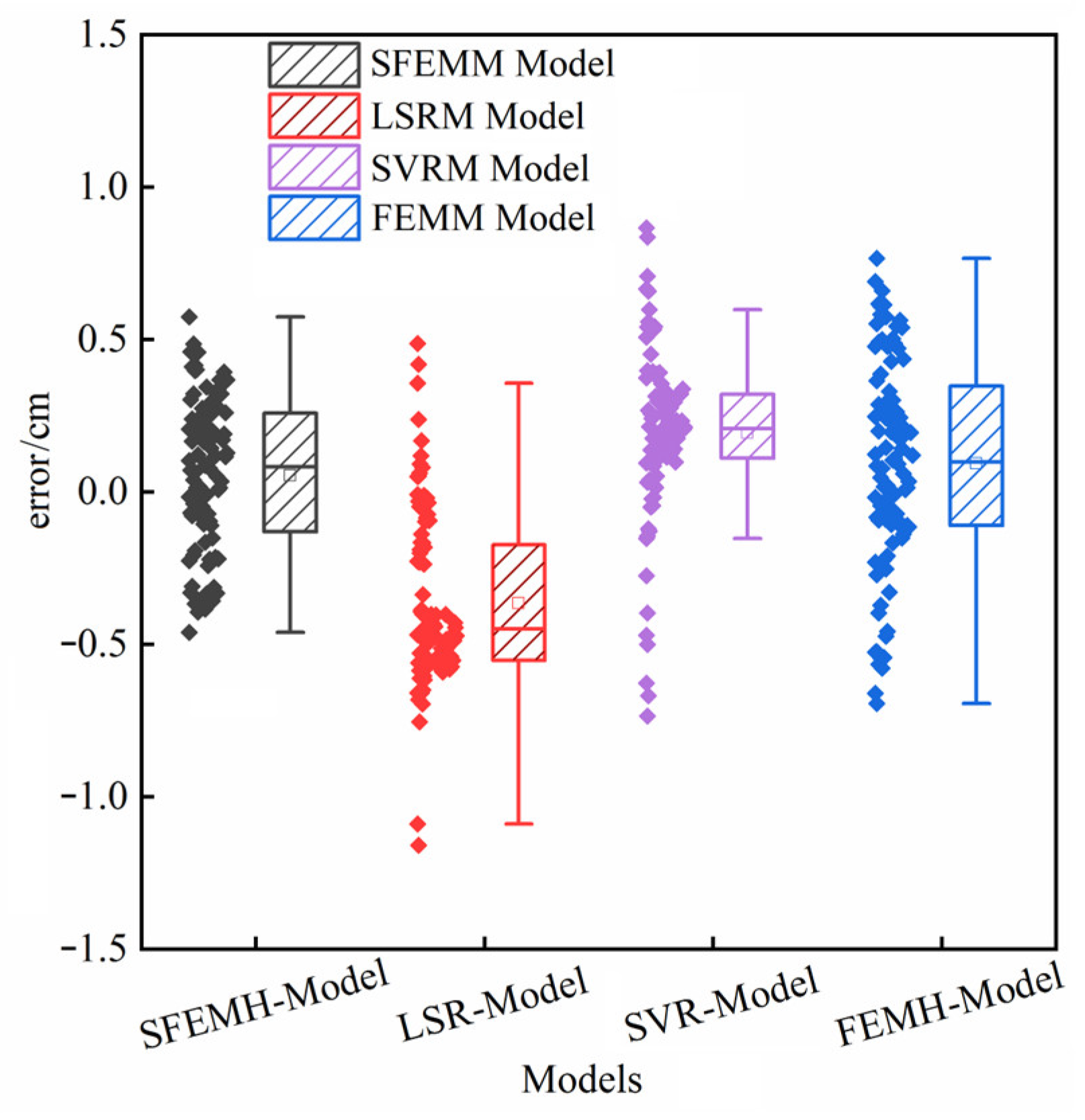
In order to more intuitively represent the distribution of prediction errors of each model, box plots are used for error comparison and a quantitative analysis of the prediction accuracy of each model. Figure 11 shows the box plots of predicted errors for each model. It can be seen from the figure that the following applies: (1) There are significant differences in the error distribution of predicted values among the four models. Compared to other models, the SFEMM model predicts a shorter error box, smaller interquartile range, and more concentrated error distribution, all within 1.5 times the interquartile range (IQR), with almost no outliers present, indicating that the SFEMM model achieves high stability in accuracy. (2) Compared to the other models, the SFEMM model predicts that the mean and median errors are closer to 0, indicating that the SFEMM model achieves higher prediction accuracy and good prediction performance.
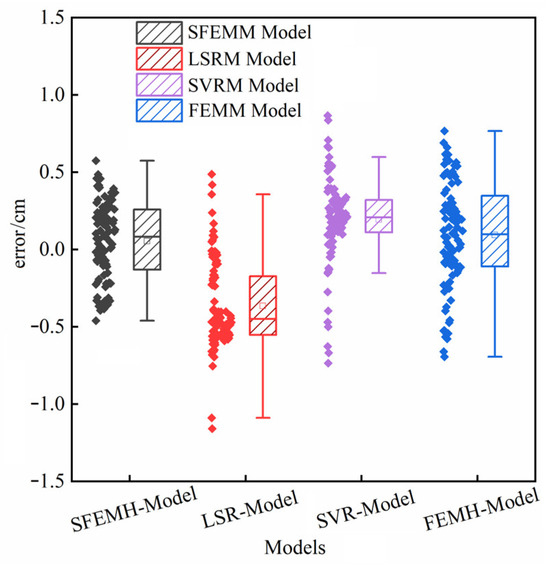
Figure 11.
Box plots of predicted errors for each model.
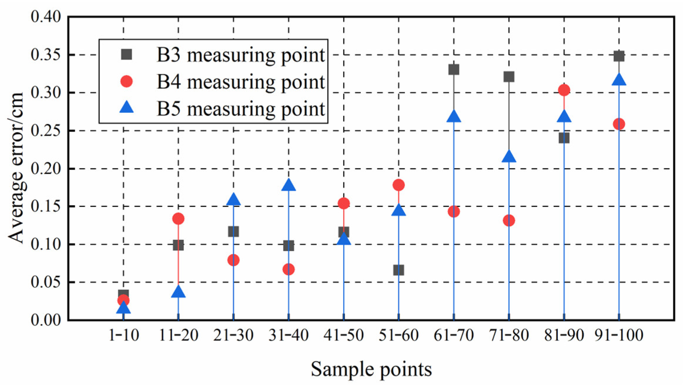
To show the applicability and stability of the SFEMM model under different measurement points more intuitively, a monitoring model is established for the horizontal displacement of the B4 and B5 measuring points of the rockfill dam, and the trend of its displacement is predicted. Figure 12 shows the model prediction accuracy of each measuring point. (1) Similar to point B3, the prediction errors of the SFEMM models at points B4 and B5 increased with the increase in the amount of predicted data, further indicating that the amount of model-predicted data should be controlled to ensure their high accuracy. (2) The overall prediction effect of the first 60 sets of displacements at points B3 and B5 is better than that of the subsequent ones, and the prediction error of the first 80 sets of displacements at point B4 is less than 0.2 cm. The above results indicate that the SFEMM model achieves similar prediction accuracy for different point displacements, and the accuracy decreases as the amount of predicted data increases. Therefore, when predicting the displacement of different measuring points, the maximum amount of predicted data should be set to ensure the accuracy and credibility of the calculation results. Based on the above analysis results, when the maximum predicted data volume should be within 60–80 sets, the error can be basically guaranteed to be less than 0.2 cm, and the analysis effect is optimal.
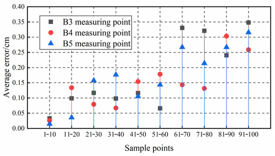
Figure 12.
Prediction accuracy of SFEMM model at different measurement points.
As shown above, this model offers advantages, such as small predictive errors, high predictive accuracy and stability, and a high correlation and similarity of the distribution shapes between predictions and measurements. The SFEM model is highly feasible and superior to other models in predicting the displacement of rockfill dams.
3.3.2. Determination of Monitoring Index
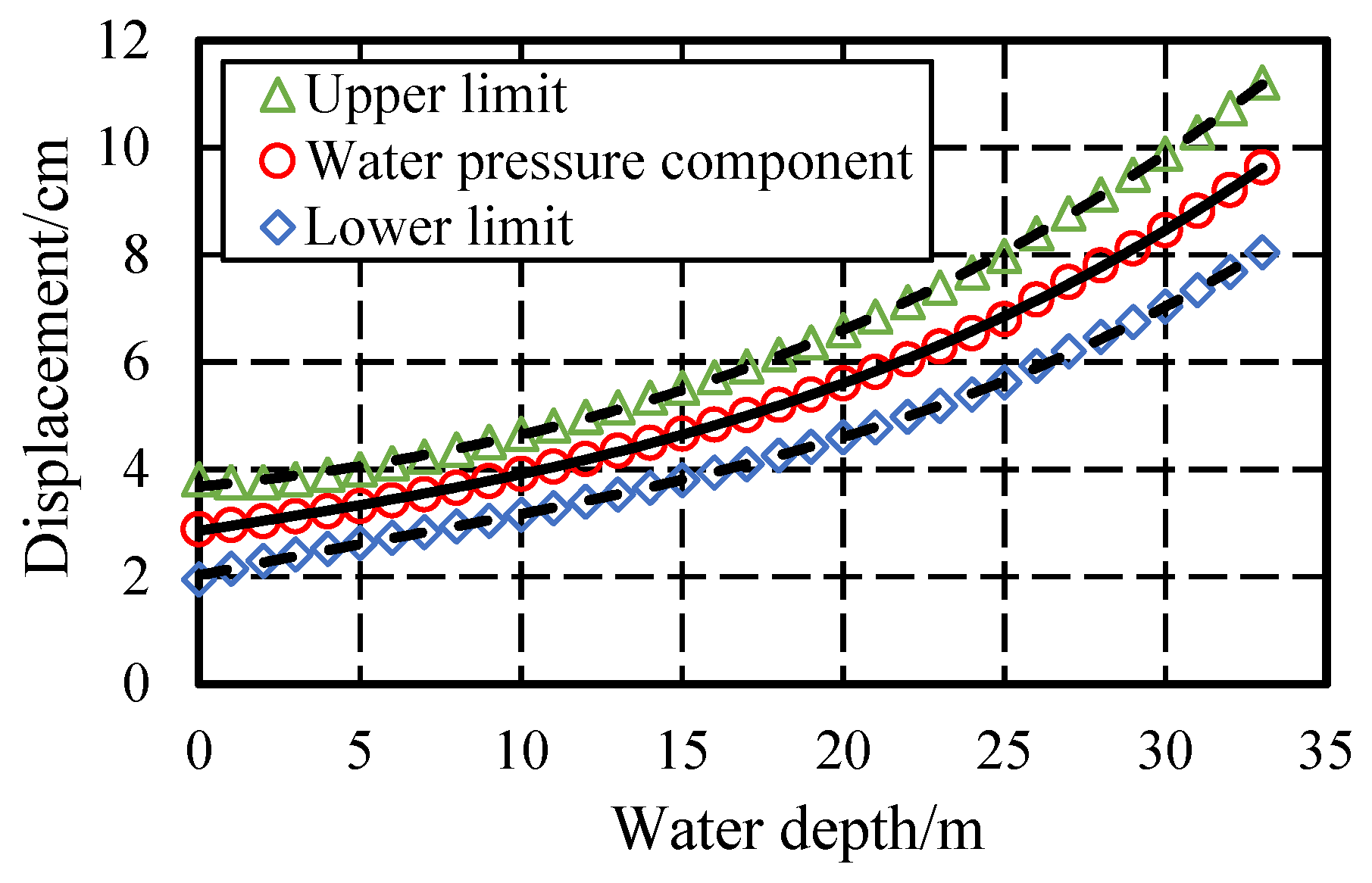
The method in Section 2.2.2 of this paper is used to determine the monitoring index of horizontal displacement at monitoring point B3. Based on the probability density distribution of horizontal displacement at monitoring point B3 of the dam obtained from SFEM at each water level, the upper and lower limits of the water pressure component at the significance level of α = 5% are determined (shown in Figure 13) and fitted with the expressions shown in Equation (14). Subsequently, the expressions for the upper and lower limits of the water pressure component are substituted into the trained SFEMM model in Section 3.3.1 to obtain the displacement monitoring index of the rockfill dam.

Figure 13.
Upper and lower limits of water pressure components and their fitting curves.
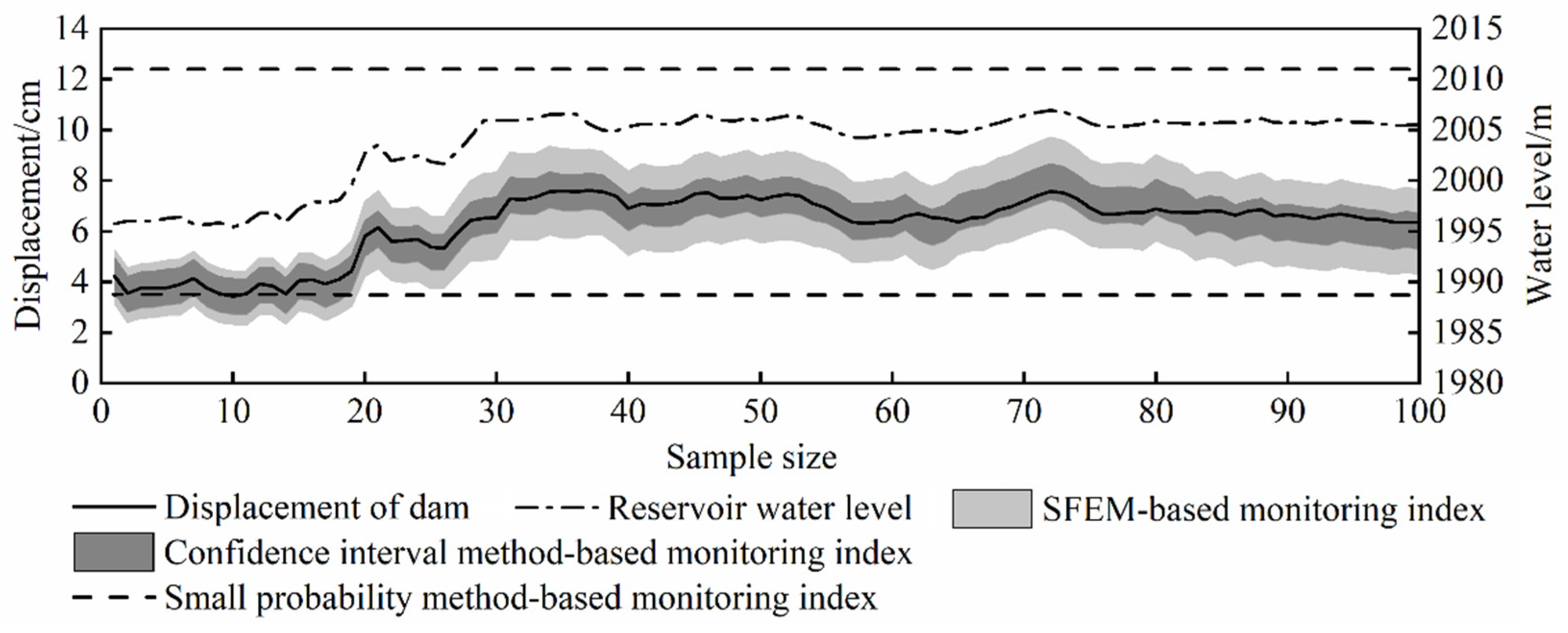
Figure 14 shows the comparison of SFEM-based monitoring index with the monitoring indexes of the traditional confidence interval method and small probability method (significance level of α = 5%). (1) Because of the accurate prediction result of SFEMM model, the measured displacements are located in the interval of the hybrid monitoring index, and the measured displacements are also in the range of the monitoring index of confidence interval method, which indicates that the dam displacement changes are normal, and the conclusion is consistent with the actual operation pattern of the project. (2) Compared with the traditional confidence interval method, the range of SFEM-based monitoring index is slightly larger than the range of monitoring index of the confidence interval method. This is because the SFEM-based monitoring index takes into account the physical and mechanical relationship between rockfill dam materials and displacement, which can better reflect the probability distribution of dam displacement under different loads, reducing excessive early warning situations in displacement monitoring in practical applications. (3) Comparing the SFEM-based monitoring index with the traditional small probability method-based monitoring index, due to the obvious trend change in the displacement of the B3 measuring point (shown in Figure 4 or Figure 5), reveals that the monitoring index of the traditional small probability method based on mathematical statistics has poor applicability and less rationality to the displacement of this measuring point. For example, in the first 20 sets of displacement measurements, there is a part of the measured value close to or even smaller than the lower limit of the monitoring index.

Figure 14.
Comparison of monitoring indexes.
4. Conclusions
This paper has proposed a new method for formulating a monitoring index to address the problem of deviation in monitoring indexes caused by the neglect of material uncertainty in traditional safety monitoring methods, which makes it difficult to accurately and comprehensively determine the true operational status of reactor rock dams. The method adopts the correlated log-normal random field to simulate the uncertainty of the parameters, and it determines the water pressure component through the SFEM and then establishes the SFEMM model. Then, based on the probability density distribution of the dam displacement at different reservoir levels, the boundary value of the displacement confidence interval is calculated, and thus, the monitoring index of the dam displacement is determined. The significance of each physical factor in this method is clear, and the index determination process is efficient and reasonable. By actual engineering case analysis, there are some main conclusions, as follows:
(1) The SFEMM model established in this paper, considering the uncertainty of the rockfill material, achieves smaller errors in the prediction of the dam displacement, higher prediction accuracy, and a more realistic distribution of the predicted values, compared with other monitoring models. In addition, the variation in the displacement prediction error for different measuring points is small, and the prediction stability is strong, showing the high accuracy and applicability of the model.
(2) In establishing the SFEMM model, the minimum sample size for analyzing and calculating should be larger than 400 sets to ensure that the probability density distribution of the dam displacement has a high stability. When the predicted sample size is within 60~80 sets, the prediction accuracy of the model is at a high level.
(3) The method proposed in this paper to determine the monitoring index links the structural deformation characteristics and utilizes SFEM to build the water pressure component to consider the material parameters uncertainty of the rockfill, reflecting the deformation mechanism of the dam body more realistically and accurately. The determined monitoring index achieves higher accuracy and adaptability compared to the traditional method, and the monitoring interval is more scientific and reasonable, reducing the waste of human resources caused by multiple warnings. It has a sufficient theoretical basis and a better application effect.
(4) It is worth discussing that both the SFEMM model and its corresponding monitoring indexes are based on SFEM analysis results; therefore, the accuracy of the SFEM results has a significant impact on the former. When there are errors in the parameter values, unreasonable random field parameters, and insufficient simulation quantities, the accuracy of the established SFEMM model is inevitably reduced, and even the error is greater than that of traditional statistical models. When there is significant uncertainty in parameter values, parameter inversion can be used to obtain relatively accurate parameter reference values. In addition, the specific impact of parameter values and random field parameters on the accuracy of SFEMM models still requires further exploration by the authors.
Author Contributions
Conceptualization, L.R. and M.L.; data curation, L.R. and Y.S.; formal analysis, L.R. and M.L.; investigation, Y.S. and S.D.; methodology, L.R. and M.L.; software, L.R. and C.M.; validation, S.D. and J.Y.; writing—original draft, L.R.; writing—review and editing, J.Y. and C.M. All authors have read and agreed to the published version of the manuscript.
Funding
This research was funded by the National Natural Science Foundation of China (No. 52279140) and the General Program of Natural Science Basic Research Program of Shaanxi (Youth) (No. 2023-JC-QN-0562).
Institutional Review Board Statement
Not applicable.
Informed Consent Statement
Not applicable.
Data Availability Statement
The original contributions presented in the study are included in the article; further inquiries can be directed to the corresponding author.
Acknowledgments
The authors are grateful to Powerchina Northwest Engineering Co., Ltd., and Xi’an University of Technology.
Conflicts of Interest
Authors Li Ran, Meng Li, Yang Sun, Shuo Ding were employed by Powerchina Northwest Engineering Co., Ltd. The remaining authors declare that the research was conducted in the absence of any commercial or financial relationships that could be construed as a potential conflict of interest.
References
- Yao, Y.; Wang, F.; Yang, Z. New development of dam construction technology with complex material for high earth-rock dam. Water Power 2023, 49, 65–71. [Google Scholar]
- Wang, S.; Xu, C.; Gu, C.; Su, H.; Hu, K.; Xia, Q. Displacement monitoring model of concrete dams using the shape feature clustering-based temperature principal component factor. Struct. Control Health Monit. 2020, 27, e2603. [Google Scholar] [CrossRef]
- Li, Z.; Hou, H. Theory and Methods on Dam Safety Monitoring Indexes. Water Power 2010, 36, 64–67. [Google Scholar]
- Li, B.; Yang, J.; Hu, D. Dam monitoring data analysis methods: A literature review. Struct. Control Health Monit. 2020, 27, e2501. [Google Scholar] [CrossRef]
- Ran, L.; Yang, J.; Zhang, P.; Wang, J.; Ma, C.; Cui, C.; Cheng, L.; Wang, J.e.; Zhou, M. A hybrid monitoring model of rockfill dams considering the spatial variability of rockfill materials and a method for determining the monitoring indexes. J. Civ. Struct. Health Monit. 2022, 12, 817–832. [Google Scholar] [CrossRef]
- Huang, Y.; Wan, Z. Study on Viscoelastic Deformation Monitoring Index of an RCC Gravity Dam in an Alpine Region Using Orthogonal Test Design. Math. Probl. Eng. 2018, 2018, 8743505. [Google Scholar] [CrossRef]
- Deng, Z.; Gao, Q.; Huang, M.; Wan, N.; Zhang, J.; He, Z. From data processing to behavior monitoring: A comprehensive overview of dam health monitoring technology. Structures 2025, 71, 108094. [Google Scholar] [CrossRef]
- Zhang, W.; Li, H.; Shi, D.; Shen, Z.; Zhao, S.; Guo, C. Determination of Safety Monitoring Indices for Roller-Compacted Concrete Dams Considering Seepage–Stress Coupling Effects. Mathematics 2023, 11, 3224. [Google Scholar] [CrossRef]
- Li, B. Research on Intelligent Analysis Method for Deformation Monitoring of Gravity Dam. Doctoral Thesis, Xi’an University of Technology, Xi’an, China, 2021. [Google Scholar]
- Wu, Z. Theory and Application of Safety Monitoring for Hydraulic Structures; Higher Education Press: Beijing, China, 2003. [Google Scholar]
- Thomas, F.; Marwan, E.M.; Ghilman, D.; Wolfgang, G.P.; Rene, B. Method for indirect determination of soil parameters for numerical simulation of dikes and earth dams. Appl. Water Sci. 2022, 12, 245. [Google Scholar] [CrossRef]
- Yu, X.; Li, Z.; Wang, Y.; Pang, R.; Lv, X.; Fu, M. Stress–deformation analysis of concrete anti-seepage structure in earth-rock dam on overburden considering spatial variability of geomechanical parameter. Probabilistic Eng. Mech. 2025, 79, 103725. [Google Scholar] [CrossRef]
- Chi, S.; Feng, W.; Jia, Y.; Zhang, Z. Application of the soil parameter random field in the 3D random finite element analysis of Guanyinyan composite dam. Case Stud. Constr. Mater. 2022, 17, e01329. [Google Scholar] [CrossRef]
- Sun, Y.; Huang, J.; Jin, W.; Sloan, S.W.; Jiang, Q. Bayesian updating for progressive excavation of high rock slopes using multi-type monitoring data. Eng. Geol. 2019, 252, 1–13. [Google Scholar] [CrossRef]
- Pang, R.; Yang, Y.; Zhou, Y.; Jing, M.; Xu, B. Seismic reliability analysis of high earth-rockfill dams subjected to mainshock-aftershock sequences using a novel noninvasive stochastic finite element method. Soil Dyn. Earthq. Eng. 2024, 183, 108817. [Google Scholar] [CrossRef]
- Chi, S.; Feng, W.; Jia, Y.; Zhang, Z. Stochastic Finite-Element Analysis of Earth–Rockfill Dams Considering the Spatial Variability of Soil Parameters. Int. J. Geomech. 2022, 22, 04022224. [Google Scholar] [CrossRef]
- Song, Z.; Han, P.; Ma, C.; Zhang, H. Inversion Analysis of Dynamic Parameters of High Panel Rockfill Dams Considering Concept of Uncertaint. Water Resour. Power 2023, 41, 118–122. [Google Scholar] [CrossRef]
- Wang, B.W.; Li, D.Q.; Tang, X.S. Impact of statistical uncertainty in soil parameters on slopestability reliability of rockfill dams. Eng. J. Wuhan Univ. 2019, 52, 758–766. [Google Scholar] [CrossRef]
- Lu, X.; Zhu, S. Stochastic Finite Element Analysis of Rockfill Dam Considering Spatial Variability of Gradation Parameters. Water Power 2022, 48, 81–89. [Google Scholar]
- Wang, J.; Yang, J.; Cheng, L.; Ma, C.; Ran, L. Study on the noninvasive stochastic finite element method of rockfill damconsidering spatial variability of material parameters. J. Water Resour. Water Eng. 2019, 30, 200–207. [Google Scholar] [CrossRef]
- Lumb, P. The variability of natural soils. Can. Geotech. J. 1966, 3, 74–97. [Google Scholar] [CrossRef]
- Stefanou, G. The stochastic finite element method: Past, present and future. Comput. Methods Appl. Mech. Eng. 2008, 198, 1031–1051. [Google Scholar] [CrossRef]
- Tanapalungkorn, W.; Yodsomjai, W.; Keawsawasvong, S.; Nguyen, T.S.; Oye, W.C.; Likitlersuang, S. Stability analysis of tunnel heading in clay with nonstationary random fields of undrained shear strength. Probabilistic Eng. Mech. 2024, 78, 103692. [Google Scholar] [CrossRef]
- Wu, C.; Wang, Z.; Goh, S.H.; Zhang, W. Comparing 2D and 3D slope stability in spatially variable soils using random finite-element method. Comput. Geotech. 2024, 170, 106324. [Google Scholar] [CrossRef]
- Liao, K.; Wu, Y.; Miao, F.; Pan, Y.; Beer, M. Probabilistic risk assessment of earth dams with spatially variable soil properties using random adaptive finite element limit analysis. Eng. Comput. 2022, 39, 3313–3326. [Google Scholar] [CrossRef]
- Shiau, J.; Nguyen, T.; Hung, T.P.T.; Sugawara, J. Probabilistic assessment of passive earth pressures considering spatial variability of soil parameters and design factors. Sci. Rep. 2025, 15, 4752. [Google Scholar] [CrossRef]
- Keshmiri, E.; Ahmadi, M.M. Reliability Analysis of Circular Foundations on Unsaturated Soils Using Monte Carlo Simulation. Geotech. Geol. Eng. 2025, 43, 111. [Google Scholar] [CrossRef]
- Deng, Z.P.; Zhong, M.; Pan, M.; Jiang, S.H.; Niu, J.T.; Zheng, K.H. Reliability Evaluation of Slopes Considering Spatial Variability of Soil Parameters Based on Efficient Surrogate Model. ASCE-ASME J. Risk Uncertain. Eng. Syst. Part A Civ. Eng. 2024, 10, 04023057. [Google Scholar] [CrossRef]
- Guo, X.; Sun, Q.; Dias, D.; Antoinet, E. Probabilistic assessment of an earth dam stability design using the adaptive polynomial chaos expansion. Bull. Eng. Geol. Environ. 2020, 79, 4639–4655. [Google Scholar] [CrossRef]
- Chen, D.; Xu, D.; Ren, G.; Jiang, Q.; Liu, G.; Wan, L.; Li, N. Simulation of cross-correlated non-Gaussian random fields for layered rock mass mechanical parameters. Comput. Geotech. 2019, 112, 104–119. [Google Scholar] [CrossRef]
- Jiang, S.; Li, D.; Zhou, C.; Fang, G. Slope reliability analysis considering effect of autocorrelation functions. Chin. J. Geotech. Eng. 2014, 36, 508–518. [Google Scholar]
- Jiang, S.; Li, D.; Zhang, L.; Zhou, C. Slope reliability analysis considering spatially variable shear strength parameters using a non-intrusive stochastic finite element method. Eng. Geol. 2014, 168, 120–128. [Google Scholar] [CrossRef]
- Luo, N.; Agarwal, E. Seismic stability and failure mechanisms of gentle and steep slopes considering soil rotated anisotropy and spatial variability. Soil Dyn. Earthq. Eng. 2024, 183, 108821. [Google Scholar] [CrossRef]
- Jiang, S.; Li, J.; Huang, J.; Zhou, C. Spatial variability characterization of the mechanical parameters of structural planes and reliability analysis of rock slopes. Chin. J. Rock Mech. Eng. 2022, 41, 2834–2845. [Google Scholar] [CrossRef]
- Tian, J.; Luo, Y.; Lu, X.; Li, Y.; Chen, J. Physical data-driven modeling of deformation mechanism constraints on earth-rock dams based on deep feature knowledge distillation and finite element method. Eng. Struct. 2024, 307, 117899. [Google Scholar] [CrossRef]
- Liu, X.; Li, Z.; Sun, L.; Yahya, K.E.; Wang, J.; Lu, W. A critical review of statistical model of dam monitoring data. J. Build. Eng. 2023, 80, 108106. [Google Scholar] [CrossRef]
- Gu, C.; Wu, Z. Theory and Methods of Dam and Foundation Safety Monitoring and Their Applications; Hohai University Press: Nanjing, China, 2006. [Google Scholar]
- Zhu, B.; Pei, H.; Yang, Q. Reliability analysis of submarine slope considering the spatial variability of the sediment strength using random fields. Appl. Ocean Res. 2019, 86, 340–350. [Google Scholar] [CrossRef]
- Ran, L.; Yang, J.; Ma, C.; Cheng, L.; Zhou, M. Global sensitivity analysis of parameters based on sPCE: The case study of a concrete face rockfill dam in northwest China. PLoS ONE 2023, 18, e0290665. [Google Scholar] [CrossRef]
- Wu, C.B.; Yan, Q. Sensitivity Analysis of Duncan E-B Model Parameters for Rockfill. Water Resour. Power 2010, 28, 94–96. [Google Scholar]
- Yang, Y.S.; Liu, X.S.; Zhao, J.M.; Wang, X.-G. Parameter sensitivity analysis of Duncan E-B model. J. China Inst. Water Resour. Hydrpower Res. 2013, 11, 81–86. [Google Scholar] [CrossRef]
- Li, X.; Li, Y.; Lu, X.; Wang, Y.; Zhang, H.; Zhang, P. An online anomaly recognition and early warning model for dam safety monitoring data. Struct. Health Monit. 2019, 19, 796–809. [Google Scholar] [CrossRef]
- Hui, C. Refined Numerical Simulation of Structural Behaviors for High Earth-Rockfill Dam with Considering Real Construction Quality. Doctoral Thesis, Tianjin University, Tianjin, China, 2018. [Google Scholar]
- Zhang, F.; Zhou, Q.; Du, P. Seismic Response Analysis of Cut-Off Wall of Dam Foundation Under Spatial Variability of Parameters. J. Shanghai Jiao Tong Univ. 2022, 56, 684–692. [Google Scholar] [CrossRef]
- Wen, D. The Study on Characteristics of Stress and Deformation of Separated Face Slabs of CFRD. Master’s Thesis, Xinjiang Agricultural University, Urumqi, China, 2015. [Google Scholar]
- Dong, J. Study on Mechanical Properties of Interface Between Soil and Structure. Master’s Thesis, Dalian University of Technology, Dalian, China, 2011. [Google Scholar]
- Feng, W.; Chi, S.; Jia, Y. Random finite element analysis of a clay-core-wall rockfill dam considering three-dimensional conditional random fields of soil parameters. Comput. Geotech. 2023, 159, 105437. [Google Scholar] [CrossRef]
- Chen, H.; Liu, D. Stochastic finite element analysis of rockfill dam considering spatial variability of dam material porosity. Eng. Comput. 2019, 36, 2929–2959. [Google Scholar] [CrossRef]
- Tan, X.; Wang, X.; Khoshnevisan, S.; Hou, X.; Zha, F. Seepage analysis of earth dams considering spatial variability of hydraulic parameters. Eng. Geol. 2017, 228, 260–269. [Google Scholar] [CrossRef]
- Sadeghian, N.; Estalaki, A.M.; Calamak, M. Probabilistic internal erosion analysis in stratified and unstratified foundations of embankment dams using copulas. Nat. Hazards 2024, 120, 12989–13007. [Google Scholar] [CrossRef]
- Ma, C. Intelligent Inversion Analysis of Macro- and Micro-Parameters of Rockfill Based on Discrete Element Method and It’s Engineering Application. Doctoral Thesis, Xi’an University of Technology, Xi’an, China, 2020. [Google Scholar]
- Zewdu, B.A.; Kegne, B.S.; Dessie, W.M.; Asrat, A.N. A Comparative Evaluation of Seepage and Stability of Embankment Dams Using GeoStudio and Plaxis Models: The Case of Gomit Dam in Amhara Region, Ethiopia. Water Conserv. Sci. Eng. 2022, 7, 429–441. [Google Scholar] [CrossRef]
- Mehdi, R.M.; Hossien, R. Uncertainty analysis in probabilistic design of detention rockfill dams using Monte-Carlo simulation model and probabilistic frequency analysis of stability factors. Environ. Sci. Pollut. Res. Int. 2022, 30, 28035–28052. [Google Scholar] [CrossRef]
- Gullnaz, S.; Azzeddine, S. Deep Neural Network and Polynomial Chaos Expansion-Based Surrogate Models for Sensitivity and Uncertainty Propagation: An Application to a Rockfill Dam. Water 2021, 13, 1830. [Google Scholar] [CrossRef]


Disclaimer/Publisher’s Note: The statements, opinions and data contained in all publications are solely those of the individual author(s) and contributor(s) and not of MDPI and/or the editor(s). MDPI and/or the editor(s) disclaim responsibility for any injury to people or property resulting from any ideas, methods, instructions or products referred to in the content. |
© 2025 by the authors. Licensee MDPI, Basel, Switzerland. This article is an open access article distributed under the terms and conditions of the Creative Commons Attribution (CC BY) license (https://creativecommons.org/licenses/by/4.0/).