1. Introduction
Over the past decade, deep networks have achieved remarkable success in the field of computer vision. Extracting local features on an image and then pooling them into a global representation has become one of the most promising types of network architectures [
1,
2,
3]. As one of the most common pooling methods, bilinear pooling aggregates local features into a matrix where correlations between different features are preserved. With their higher-order information, the enriched representations have been used in various tasks [
4,
5,
6,
7], especially in visual recognition [
8,
9,
10,
11,
12].
Among bilinear pooling approaches, normalizing bilinear representation is almost applied, and is considered as an indispensable step to further boost performance [
13]. Existing normalization approaches can be roughly categorized into element-wise normalization and structure-wise normalization.
Element-wise normalization was first proposed to suppress the burstiness of bag-of-words features [
14], and was then found to be effective in bilinear pooling as well. For each element in bilinear representation, the approach in [
13] normalizes it by its square root and then divides the result by its Frobenius norm. This kind of normalization is simple yet effective and, thus, is widely used in bilinear pooling approaches [
9,
13,
15,
16,
17].
Structure-wise normalization considers the fact that bilinear representation is a Symmetric Positive Definite matrix whose space forms a Riemannian manifold. Thus, it is clearly sub-optimal to send the representation to a linear classifier. The representation should be normalized by mapping the manifold into an Euclidean space. In particular, the O2P method [
18] applies the matrix logarithm function as the normalization which can improve performance. In the following, DeepO2P [
19] proposes back-propagation of the matrix logarithm function and achieves end-to-end learning of deep networks. However, computing matrix logarithm and its gradient are less efficient on the GPU. To accelerate the normalization, other works [
15,
20,
21] suggest the square root of an SPD matrix which can also complete the linear mapping [
22]. More importantly, the square root process can be approximated by Newton’s iteration [
15] where only basic matrix–matrix multiplications are involved. Therefore, the normalization with Newton’s iteration is GPU-supported, and its efficiency has made itself one of the major normalization approaches to bilinear pooling. Although Newton’s iteration provides strong theoretical support and good performance [
15,
22], its sequential matrix multiplications still result in a high computational complexity of
, where
D is feature dimension and is always large (
for ResNet-50 network [
1]) for modern deep network architectures. Thus, more efficient structure-wise methods are further studied. For example, Run [
23] only normalizes the largest eigenvalue and simplifies the computation into matrix–vector multiplications. PSMR [
9] can reduce computational complexity into
. Here,
N is the number of local features and can be smaller than the feature dimension in most cases. iSICE [
8] and iSQRT [
20] adopt a convolutional layer to reduce feature dimension before bilinear pooling. Although great efforts are made, the aforementioned studies make a trade-off between the efficiency and recognition accuracy of the network.
Recently, a pioneering work [
10,
24] analyzed the effect of the square root normalization and, for the first time, showed that the normalization reaches a good balance between feature decorrelation and information preservation. According to this finding, its method, called DropCov, achieves normalization by applying an adaptive channel dropout to the features before bilinear pooling. Therefore, compared with the square root normalization, this method only has a linear complexity of
and is free of inference, largely improving the efficiency while keeping good recognition accuracy.
Although DropCov is impressive, it is highly dependent on the channel dropout rate. A small dropout rate can lead to nearly no normalization for bilinear representation and a high dropout rate can make the network fail to converge. To solve this problem, the work [
10] proposes a network branch that predicts the dropout rate. Therefore, the rate can be adaptively set for each training sample when the training is proceeding. However, the branch is parametric and needs sufficient training data for accurate predictions. In
Section 4.2, we observe its lower robustness on small-scale benchmarks (such as Caltech-UCSD Birds-200-2011 [
25]). Furthermore, as a variant of the original dropout [
26], DropCov samples a random subset of convolutional filters to be trained every iteration and makes the network converge slowly [
27]. As a result, although DropCov has linear complexity
during training, in certain cases, the training needs more epochs and spends more time than square root normalization.
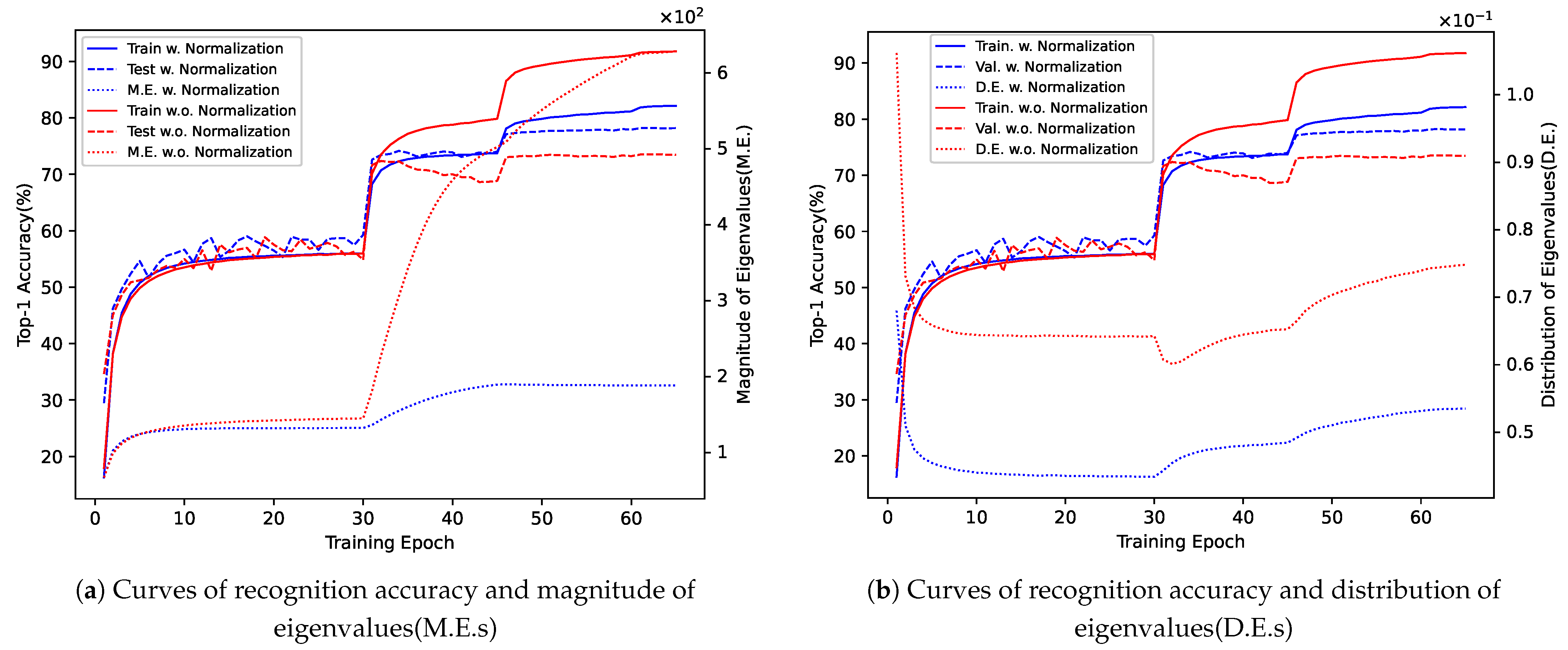
The above disadvantages of previous works motivated us to design a more efficient and robust approach to normalize the bilinear representation matrix. Inspired by original square root normalization, whose square root mainly changes the distribution and magnitude of eigenvalues, we hypothesize that the distribution and magnitude of eigenvalues play an important role in the normalization. To prove this hypothesis, we quantified the distribution of eigenvalues (D.E.s) and magnitude of eigenvalues (M.E.s) as two scalars. More details about D.E.s and M.E.s can be found in
Section 3.3. Then, we trained two networks, respectively, with and without square root normalization on ImageNet1K [
28] dataset. In
Figure 1, we show four quantities as a function of training epochs—(1) Training (Train.) accuracy, (2) Validation (Val.) accuracy, (3) M.E.s, and (4) D.E.s. As illustrated, with the normalization (blue curves), the network avoids severe overfitting and achieves higher accuracy, compared to the one without normalization (red curves). More interestingly, the normalization effectively suppresses the values of M.E.s and D.E.s, making the sum of eigenvalues smaller and the distribution less peaky. This phenomenon also conforms to the change in the eigenvalues when applying the normalization: the eigenvalues are square-rooted. Generally speaking, the normalization correlates with M.E.s and D.E.s. Suppressing M.E.s and D.E.s to some extent may avoid overfitting and result in better network performance. This leads to the main questions of this paper: is there another normalization that can suppress M.E.s and D.E.s rather than the original square root normalization? If so, can we replace the original square root normalization with it?
To answer these questions, in this paper, we work on regularizing M.E.s and D.E.s in the bilinear pooling matrix and studying its effect on the performance of deep networks. To this end, we propose an implicit normalization, namely RegCov, which encourages the network to align current M.E.s and D.E.s with the target ones. Different from DropCov [
10], RegCov normalizes bilinear representation by adding two regularization terms in the objective function and no more parameters are introduced. This quantity can avoid performance degeneration when training data are not sufficient. Consequently, unlike DropCov, our method can perform well on the benchmarks in various scales, especially in small scales. Secondly, RegCov also holds free computational complexity for inference. During training, our method adopts a two-stage strategy where square root normalization is initially applied because it can achieve fast training convergence. We apply the proposed method to the recent deep networks and run extensive experiments on the datasets in different scales. All cases suggest that RegCov is a robust and efficient normalization for bilinear pooling.
3. Our Approach
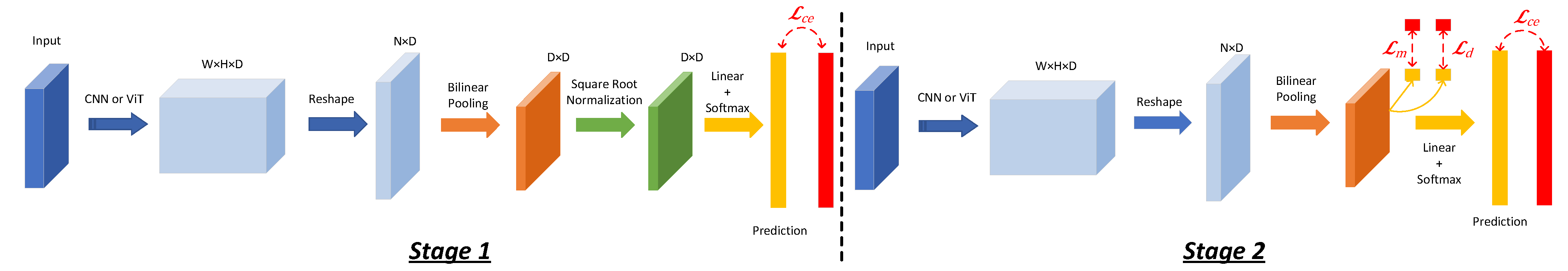
As shown in
Figure 2, a deep network, such as Convolutional Neural Network (CNN) or Vision Transformer (ViT), extracts on the image local features
, where
W,
H and
D are, respectively, width, height and feature dimension. After being reshaped, local features
are flattened into a feature matrix
, and the number of feature vectors
. Bilinear pooling aggregates these local features into bilinear representation
. Then, at the first training stage,
is processed by square root normalization, and the output matrix
is sent to a fully connected layer for final classification prediction. The network is trained with cross-entropy loss
. At the second stage, the normalization is rejected and the resulting network is continued to be trained with
and two newly proposed regularization terms:
and
. During inference time, we use the network trained after the second stage so no normalization is used.
3.1. Bilinear Pooling
At the first and second stages, a deep network extracts local features
, where
N is the number of feature vectors, and
D is their dimension. Bilinear pooling works as a global pooling approach that aggregates
into the bilinear representation
:
where
is a small value 1 ×
and adds to diagonal values in the matrix
for the sake of stability during training. Like the representation after average pooling and max pooling, the diagonal values in
also preserve representative features in each separate feature dimension. Furthermore, non-diagonal values show richer information, i.e., the correlation between each pair of dimensions. Hence, bilinear pooling is more powerful and validates its effectiveness in many computer tasks [
4,
5,
8,
9,
10,
11,
12,
19].
3.2. First Stage
Despite being powerful, the representation lies in the Riemannian manifold. Obviously, it is not adapted to a linear classifier (fully connected layer), which works in the Euclidean space. Hence, at the first stage, we perform square root normalization on the before the classifier. The solution normalizes into its square-rooted one: so that .
Originally, the normalization can be processed with the SVD [
22,
57]. Let the SVD of
be expressed as
where
is the matrix of eigenvectors, and the diagonal matrix
contains eigenvalues. The normalized matrix is obtained by square rooting diagonal elements in
:
Nevertheless, computing square-rooted matrix
via SVD is less efficient on the GPU and slows the whole training process. Alternatively, at the first stage, we use Newton’s iteration, as proposed in [
15,
20], to calculate approximated
. Specifically, it is dedicated to solving the formula
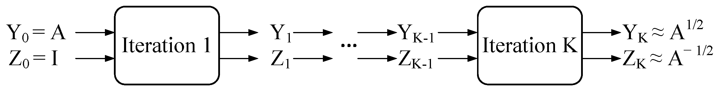
. The approach is an iterative process where each iteration is as follows:
As illustrated in
Figure 3, the inputs are
and
. After
K iterations,
and
converge to
and
. Like previous works,
K is set to be 5 throughout the paper. Furthermore, Equations (
4) and (
5) indicate that the normalization process only consists of matrix multiplications which are well supported on the GPU. Therefore, we adopt it at the first stage to speed up the normalization.
Finally, the normalized representation
is flattened as a vector and sent to a linear classifier. The network is trained with the cross-entropy loss
:
where
and
are, respectively, the target and predicted probability values at
c-class, respectively, of the
s-th training sample.
3.3. Second Stage
At the second stage, we remove the square root normalization because, although the efficiency has already been improved, Newton’s iteration still has an expensive computational complexity of , where D is the number of feature dimensions.
However, as Equation (
3) shows, square root normalization square-roots eigenvalues in the matrix
, and rejecting the normalization will change both the magnitude and distribution of eigenvalues. To quantify this change, we define the magnitude
as the sum of eigenvalues:
where
can be obtained via the trace of
. Subsequently,
is divided by
, and we have
. The sum of eigenvalues
in the matrix
is always 1. Then, the distribution of eigenvalues can be defined as the Frobenius norm of
:
The value of can enable us to decide the flatness of the distribution of eigenvalues. For example, represents the most peaky distribution where only one eigenvalue is equal to 1 and the others are zero. On the contrary, represents the most flat distribution where all the eigenvalues are equal to . Within the interval , a smaller value means a flatter distribution and vice versa.
For our approach RegCov, when the first stage terminates, we record the average distribution and magnitude values
and
for all the training samples. After the removal of square root normalization, we add two regularization terms in the loss function during training and the network is encouraged to output the bilinear representation whose
and
approach to the target
and
:
Here,
and
push current
and
of the
s-th training sample towards
and
.
and
are loss weights whose values will be further studied in
Section 4.6.
3.4. Discussion
We insist on explicit square root normalization at the first stage. The reason is that our method RegCov needs the accurate targets
and
from Equation (
9). Across different datasets and network architectures, the targets
and
can vary greatly. Inaccurate target values make bilinear representation dissimilar to the normalized one and eventually negatively influence classification performance.
In addition, the computational complexity of Newton’s iteration is
, which is much bigger than the
of the state-of-the-art approach DropCov in the training phase. This limitation slows down the training speed for each epoch. However, the following
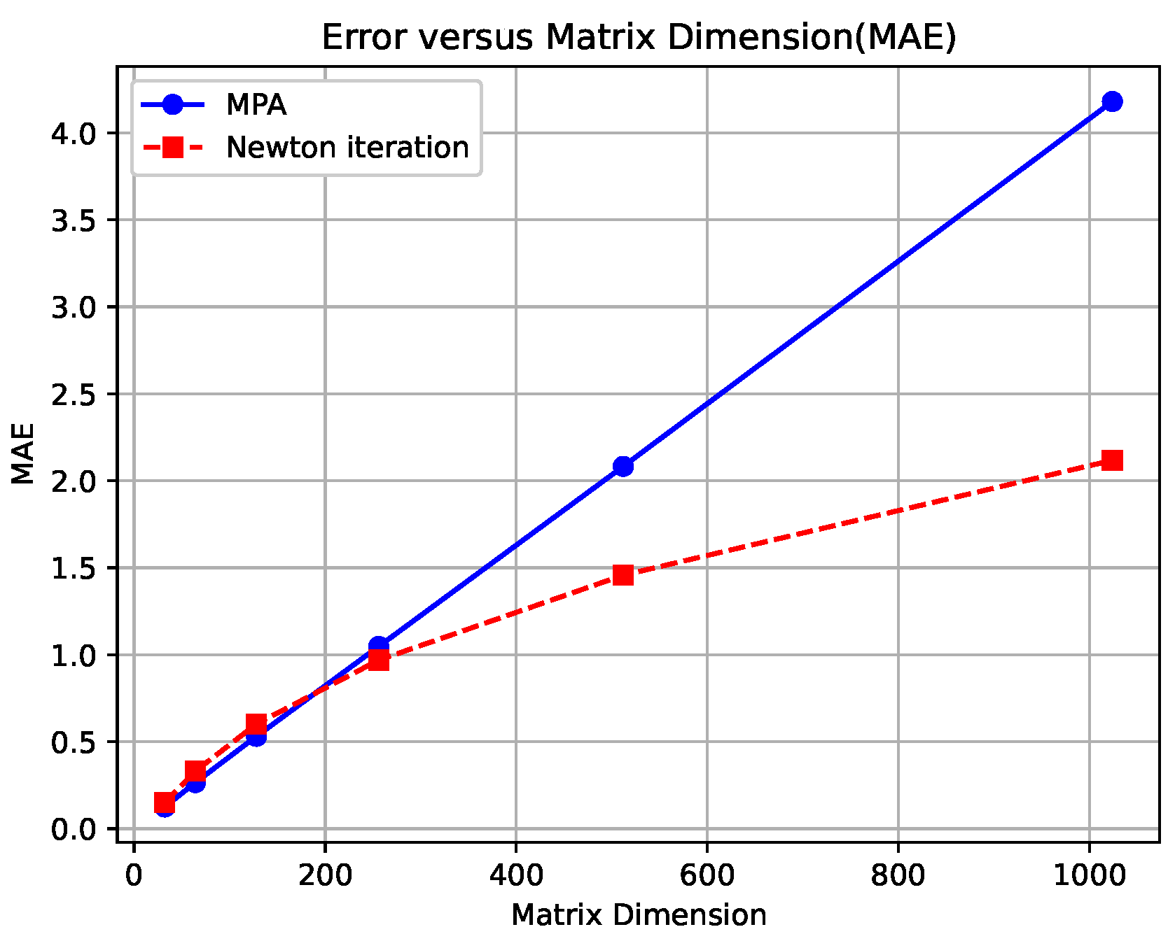
Section 4.3 will show that Newton’s iteration needs less of a training epoch. Eventually, training time spent on our network is acceptable. Moreover, by replacing Newton’s iteration with a more efficient matrix square root, called MPA [
51], the training speed of our approach can be further accelerated. In
Section 4.7, the feasibility of MPA will be studied.
Another advantage of RegCov is its efficiency at the second stage. It simplifies the alignment of eigenvalues into the regularization of two scalar values:
and
. As detailed in
Section 4.5, RegCov can result in approximated square-rooted eigenvalues. Additionally, RegCov avoids explicit calculation of each eigenvalue via computationally expensive SVD and makes the training faster.
RegCov first trains a teacher network whose bilinear pooling contains square root normalization. Then, its normalization is rejected and the resulting network is a student network that is finally trained with prior knowledge from the teacher. The above methodology makes RegCov similar to knowledge distillation (KD) [
58], where the knowledge distilled from a teacher model improves a lightweight student model. Most of the KD methods use either the teacher’s output logits [
58,
59,
60] or features from intermediate layers as distilled knowledge [
61,
62,
63,
64,
65]. Differently, RegCov only needs two scalar values from bilinear representation, making itself simple yet effective.
4. Experiments
In this section, we first describe implementation details of RegCov in
Section 4.1. In
Section 4.2, we verify the generalization of the approach by implementing it into four common pre-trained deep network backbones and by fine-tuning the networks on three fine-grained visual recognition datasets. Additionally, we train our method from scratch on a large-scale object classification dataset and compare it with other normalization methods in
Section 4.3. We also evaluate our method on a remote sensing dataset in
Section 4.4. We further investigate the effectiveness of our approach by its alignment of eigenvalues in
Section 4.5. Finally, we perform hyper-parameter analysis in
Section 4.6, computational complexity analysis in
Section 4.7, and visualization analysis in
Section 4.8.
4.1. Implementation Details
Models. For the experiments with three fine-grained visual recognition datasets, following the common settings [
9,
13,
31], we used the networks pre-trained on the ImageNet1K dataset, and extracted feature matrix
after
in the VGG-16 and before global average pooling in other networks. Subsequently, bilinear pooling of Equitation (
1) was followed, except for ResNet-50, where we applied the compact bilinear pooling of PSMR [
9] because the feature dimension
D here was too large. When training from scratch, we adopted the CNN backbones from [
8,
10,
21], where the feature dimension of
was reduced to 256 with a
convolutional layer.
Training and Evaluation. For fine-grained visual recognition tasks, we adopted the same image pre-processing techniques as those in [
20,
50] for a fair comparison. Input images were resized to 448 × 448, both for training and inference. Random horizontal flip was the only data augmentation method applied during training. The training is composed of two stages. At the first stage, we only trained the last FC layer for 100 epochs with Stochastic Gradient Descent (SGD) optimizer, whose learning rate was
, weight decay was
, and the momentum was
. Then, we fine-tuned the whole network for another 100 epochs with the initial learning rate of
and weight decay of
. The batch size was set as 32 and the learning rate was divided by 10 when the training loss remained higher than
times the current minimum loss value for 10 epochs. At the second stage, we removed the normalization part and continued to fine-tune the network for another 15 epochs. The initial learning rate was
and was reduced by 10 at the 9th epoch. For inference, we averaged the classification scores for both the input image and its flipped version as the final prediction. This setting is quite common in the bilinear pooling field [
8,
13].
For training a CNN on large-scale dataset ImageNet1K, according to refs. [
10,
20,
21], during training, a random crop was made on the original image and was then resized into 224 × 224. A random horizontal flip was also applied. At the first stage, the optimization strategy corresponded to SGD with an initial learning rate of 0.1. The network was trained within 80 epochs for ResNet-18 and 65 epochs for ResNet-50. The learning rate was decayed by 10 in the epochs 30, 60 and 75 for ResNet-18 and was decayed by 10 in the epochs 30, 45 and 60 for ResNet-50. At the second stage, the bilinear normalization was removed and the network was fine-tuned with the learning rate of 0.001, which was decayed by 10 after 9 epochs in 15 epochs in total. For inference, the input image was the center crop of 224 × 224 on the resized image whose shorter edge was matched to 256.
Throughout all the experiments, the loss weight parameters
and
in Equation (
9) changed linearly for every training iteration. For the tasks on the ImageNet1K,
increased from
to
and
increased from
to
. For the other tasks,
increased from
to
and
was the same. The studies on loss weight parameters are provided in
Section 4.6.
4.2. Experiments on Small-Scale Datasets
In this section, we evaluate the performance of the proposed approach on three fine-grained image classfication benchmarks. Caltech-UCSD Birds-200-2011 (Birds) [
25] includes 5994 images for training dataset and 5794 images for test dataset from 200 bird species. FGVC-Aircraft Benchmark (Aircrafts) [
66] consists of 100 aircraft categories, each of which has 67 training images and 33 test images. Stanford Cars (Cars) [
67] provides 16,185 images and 196 classes of cars. The Cars dataset has a rough 50–50 split per class, resulting in 8144 training images and 8041 test images.
Table 1 presents classification accuracy results and inference speed for both our approach and counterparts. The accuracy results for counterparts are all reported from the studied papers, except for DropCov, whose results are absent in its paper. Our approach achieves good balance between running speed and classification performance. When the backbone is VGG-16, our approach significantly improves the performance of BCNN by
even though the two works share the same deep network architecture. Similarly, average accuracy increases by 6.9% for ResNet-50, where our network is identical to CBP. iSICE shows very competitive accuracy results, especially for VGG-16 and ResNet-50. On average, its accuracy for VGG-16 is superior to ours. However, iSICE adopts Newton’s iteration, which eventually greatly decelerates the whole network. Even worse, to avoid high computation, iSICE reduces the feature dimension
D to 256. The reduction causes information loss from the original features and impacts negatively on the accuracy. This phenomenon is more obvious for networks ResNet-50, ResNet-101, ConvNext-T [
68], Swin-T [
69], and Swin-B [
69], whose original
D is large. Compared to iSICE, RegCov saves time from the normalization part while using the original features.
The most relevant counterpart to our approach is DropCov. Its network architecture during inference is identical to ours, so running speed is always the same. However, for classification performance, ours is superior to DropCov by a clear margin. This validates our claim that due to the lack of training samples, the network branch in DropCov is not trained sufficiently and has difficulty predicting appropriate dropout rates. On the contrary, at the first training stage of our approach, Newton’s iteration is adopted as the square root normalization approach. Unlike DropCov, Newton’s iteration is not data-driven, so it is naturally robust to small datasets. Thanks to the strong baseline, our networks are trained more effectively at the second stage where the normalization is omitted.
4.3. Experiments on ImageNet1K
We evaluate our method on large-scale image classification using the ImageNet1k dataset, which includes 1.28 M training images, 50 K validation images and 100 K testing images from 1000 classes. For a fair comparison with Dropcov, we apply Global Covariance Pooling (GCP) instead of bilinear pooling. GCP centers each feature vector
to a zero mean:
before bilinear pooling. We implemented our approach into ResNet-18 and ResNet-50, and trained the networks from scratch. The counterparts include Plain GCP [
13] (i.e., GCP without normalization), iSQRT-Cov [
20], Layer Normalization (LN) [
41] and DropCov [
10].
In
Table 2, Top-1 classification accuracy on the validation dataset, inference speed and training time are reported. Our method and plain GCP do not apply the normalization but ours clearly outperforms plain GCP in terms of accuracy with equal inference speed. Meanwhile, iSQRT-COV applies square root normalization with Newton’s iteration and achieves competitive accuracy. But its running speed is unsatisfactory due to the normalization which has a computational complexity of
. Layer Normalization is an element-wise normalization method, which normalizes each sample with its mean (
) and variance (
) and subsequently applies a linear transformation to each element. Its improvement in accuracy is marginal and consumes more inference time than ours. DropCov and RegCov achieve the best balance between inference speed and accuracy. However, for the training time, at the first stage of our method, we share the same network with iSQRT-COV. The square root normalization effectively normalizes the bilinear representation and leads to fast convergence [
20]. As for DropCov, it repeatedly samples a random subset of features for each iteration and a proportion of data could not be seen until several epochs. This behavior makes the training hard and spends more epochs for convergence [
27]. Therefore, although the square root normalization proceeds in our method, its training time is acceptable and is even smaller than DropCov for ResNet-50.
4.4. Experiments on UC Merced Dataset
We evaluated the proposed approach on the UC Merced dataset [
71], a benchmark dataset for remote sensing scene classification. This dataset comprises 21 land-use categories, with each category containing 100 scene images of size 256 × 256 × 3 pixels.
We compared the proposed method with IB-CNN [
72], which explores the application of bilinear pooling in remote sensing scene classification. For a fair comparison, we adopted the experimental settings described in [
72] and used ResNet-34 as the backbone network. Additionally, 50% of the images were randomly selected as the training dataset, while the remaining images were reserved for testing. The classification performance was evaluated using two metrics: overall accuracy (OA) and the Kappa coefficient (
). To ensure statistical reliability, each experiment was repeated five times, and the average results were reported as the final accuracy.
Table 3 summarizes the classification results. In addition to IB-CNN, the results of fine-tuned CNN (F-CNN) and bilinear CNN (B-CNN) are also included in the table. Compared to F-CNN, B-CNN achieves better performance, demonstrating that bilinear pooling improves classification accuracy. By leveraging the proposed joint pooling method, IB-CNN generates more compact bilinear representations while preventing an increase in the parameter size of the subsequent fully connected layer, which mitigates overfitting and thereby improves network performance. In contrast to IB-CNN, our RegCov method incorporates normalization, and its superior results highlight the robustness of our approach across different classification tasks. These findings further emphasize that the normalization plays a crucial role in significantly boosting performance.
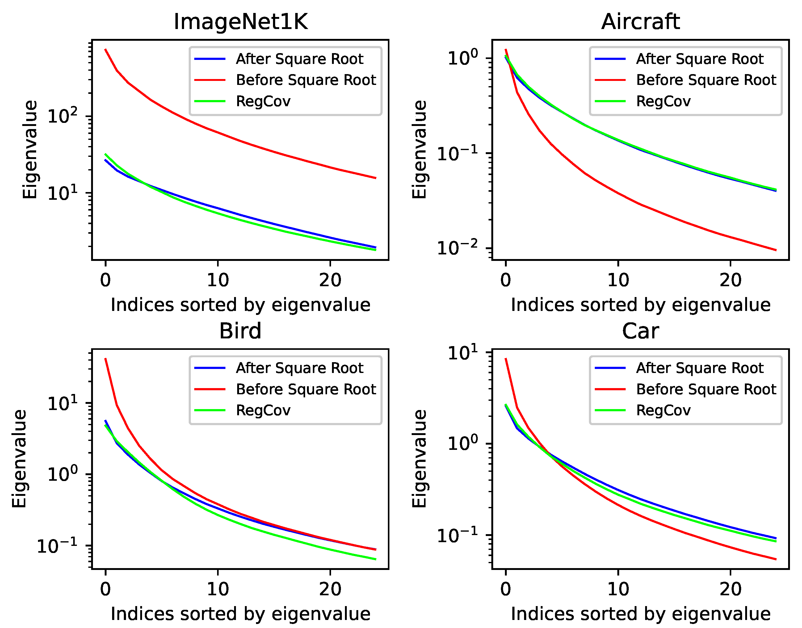
4.5. Alignment of Eigenvalues
According to Equation (
3), square root normalization produces the normalized bilinear representation matrix
by square-rooting the eigenvalues of the matrix
. Our approach, RegCov, adds regularization terms in the objective function Equation (
9) and encourages the network without the normalization to output the normalized bilinear representation. To verify,
Figure 4 plots the distribution of the largest 25 eigenvalues in the matrices
,
and the one made by our approach. For each dataset, we randomly selected 256 samples, calculated the eigenvalues of each sample, sorted them in descending order, and produced average eigenvalues across the samples. Compared to the one before square root normalization (red curves), the square root normalization considerably changes the distribution of the largest 25 eigenvalues (blue curves), making it more uniform. For our approach, RegCov succeeds in making the spectrum (green curves) close to the normalized one (blue curves). Especially for the large eigenvalues, the green and blue curves are almost overlapping. And good normalization on the principal eigenvalues is key to enhancing bilinear representation [
23,
46]. Finally, on the sample-wise level, our method can effectively reduce the distance to the eigenvalues after square root normalization, as shown in
Table 4.
4.6. Hyper-Parameter Analysis
Impact of the Number of Epochs. In
Table 5, we analyze the impact of the number of epochs at the second stage. Throughout the experiments, it takes the first
of epochs to linearly increase
and
. As observed, the accuracy stably augments when the number of training epochs increases and becomes saturated after 10 epochs. And we choose the setting of 15 epochs for all the experiments, considering the good balance between training time and network performance.
Impact of the weights and . As indicated in Equation (
9), the weights decide regularization strength and should be carefully chosen. In
Table 6, firstly, it is sub-optimal if
and
are set as zero, showing the necessity of the regularization terms. Secondly, fixed values during training bring marginal improvement. For example, high fixed values will make the regularization terms
and
dominant in Equation (
9) and lead the network to minimize classification loss
slowly. On the other hand, low fixed values cause weak regularization on bilinear representation and consequently influence the accuracy. For these reasons, we choose to linearly increase these values so that the network can focus on improving classification performance in the beginning and avoid subsequent overfitting caused by weak regularization.
4.7. Computational Complexity Analysis
Our approach can be considered as a variant of knowledge distillation. This is because RegCov employs
and
after the first training stage to guide a lighter network at the second stage. Hence, in this section, we use VGG-16 backbone on the Birds dataset and compare our approach with other knowledge distillation approaches, as shown in
Table 7. The approach of logits [
58] and Features [
61] refer to, respectively, using prediction logits and normalized bilinear representation of the network at the first stage for knowledge distillation. It can be seen that the two approaches require more training time and more parameters. This is because they should run the teacher network every training iteration. In addition, they cannot transfer exact knowledge about the eigenvalues in the bilinear representation matrix. This limits its effect of the normalization and finally results in lower accuracy. SVD calculates explicitly the eigenvalues and consumes much more training time than ours due to its poor efficiency on the GPU.
Furthermore, at the first training stage, we selected Newton Iteration as explicit square root normalization. However, as discussed in
Section 3.4, it would be important to implement a more efficient approach to compute the matrix square root. To this end, we utilized the official implementation of a state-of-the-art method, MPA [
51] and conducted experiments on the Birds dataset [
25] using the VGG-16 network. As shown in
Table 8, MPA demonstrates faster computational speeds than the Newton Iteration method during the training phase. The results are consistent with the findings in ref. [
51]. However, MPA provides lower classification accuracy in
Table 8. We found that this is attributed to the reduced accuracy of the square-rooted matrix computed by MPA, particularly when the matrix dimension is large (please see
Appendix A for details). Given that the matrix dimension in our approach RegCov is at least 256, and considering the inefficiency of SVD variants shown in
Table 8, we retain Newton Iteration.
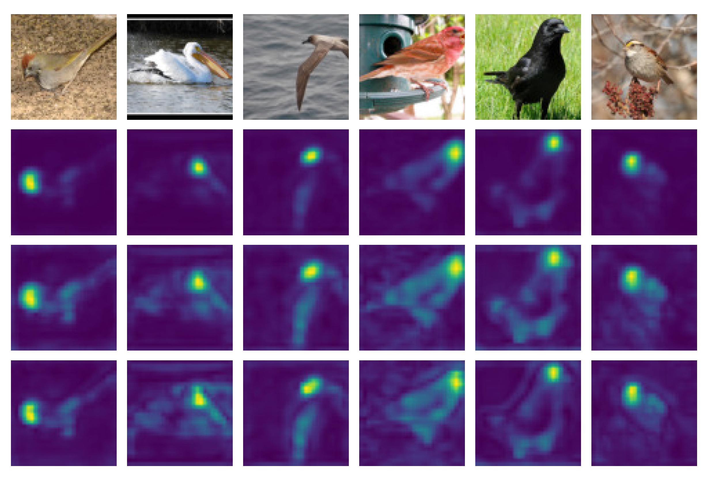
4.8. Visualization Analysis
In
Figure 5, we show the heatmap of the feature matrix
by calculating its
-norm across the channel dimension. Square root normalization suppresses dominant features and exploits more discriminative regions where corresponding features are enhanced. Our approach regularizes the features and can output similar feature heatmaps without explicit normalization.


