Pansharpening Applications in Ecological and Environmental Monitoring Using an Attention Mechanism-Based Dual-Stream Cross-Modality Fusion Network

Abstract

Pansharpening is a critical technique in remote sensing, particularly in ecological and environmental monitoring, where it is used to integrate panchromatic (PAN) and multispectral (MS) images. This technique plays a vital role in assessing environmental changes, monitoring biodiversity, and supporting conservation efforts. While many current pansharpening methods primarily rely on PAN images, they often overlook the distinct characteristics of MS images and the cross-modal relationships between them. To address this limitation, the paper presents a Dual-Stream Cross-modality Fusion Network (DCMFN), designed to offer reliable data support for environmental impact assessment, ecological monitoring, and material optimization in nanotechnology. The proposed network utilizes an attention mechanism to extract features from both PAN and MS images individually. Additionally, a Cross-Modality Feature Fusion Module (CMFFM) is introduced to capture the complex interrelationships between PAN and MS images, enhancing the reconstruction quality of pansharpened images. This method not only boosts the spatial resolution but also maintains the richness of multispectral information. Through extensive experiments, the DCMFN demonstrates superior performance over existing methods on three remote sensing datasets, excelling in both objective evaluation metrics and visual quality.

1. Introduction

Image fusion is a popular area of research in remote sensing image processing, with the goal of enhancing spatial and temporal resolution, change detection, reliability, display capabilities, and system performance robustness [1]. Remote sensing imagery offers a practical and cost-effective means for good environmental management [2], especially when large areas have to be monitored, or information is needed periodically, by measuring earth features from spectral characteristics. For example, using pansharpening to improve the resolution of remote sensing images can help researchers better identify and study natural phenomena or environmental changes [3]. As remote sensing continues to evolve, the development of advanced DL models will undoubtedly play a pivotal role in overcoming existing challenges and unlocking new possibilities for Earth observation [4]. However, remote sensing sensors cannot capture high-resolution hyperspectral images because of their inherent limitations. To be specific, they can obtain PAN and MS images separately [5]. Remote sensing satellite imaging systems grapple with the challenge of concurrently acquiring images that possess high-resolution multispectral (HRMS) images. While enhancing the hardware may address this issue, it is not a viable solution given the stringent limitations imposed by the SNR of satellite products [6]. In order to tackle this challenge, researchers have proposed the pansharpening technique. In recent years, Convolutional Neural Networks (CNNs) have become a fundamental framework in the field of computer vision, playing a crucial role in various deep-learning applications. Nevertheless, recent studies indicate that CNNs often establish short-range dependencies while overlooking global contextual information. Fortunately, Transformer models are capable of overcoming this limitation and have been broadly utilized in natural language processing (NLP) since their introduction [7]. Subsequently, their application has expanded to computer vision (CV) tasks in recent years, including pansharpening, where they demonstrate state-of-the-art (SOTA) performance. In recent studies, some researchers have tried to leverage the strengths of Transformers for pansharpening tasks. For example, Meng et al. [8] presented a network by using the transformer structure [9].

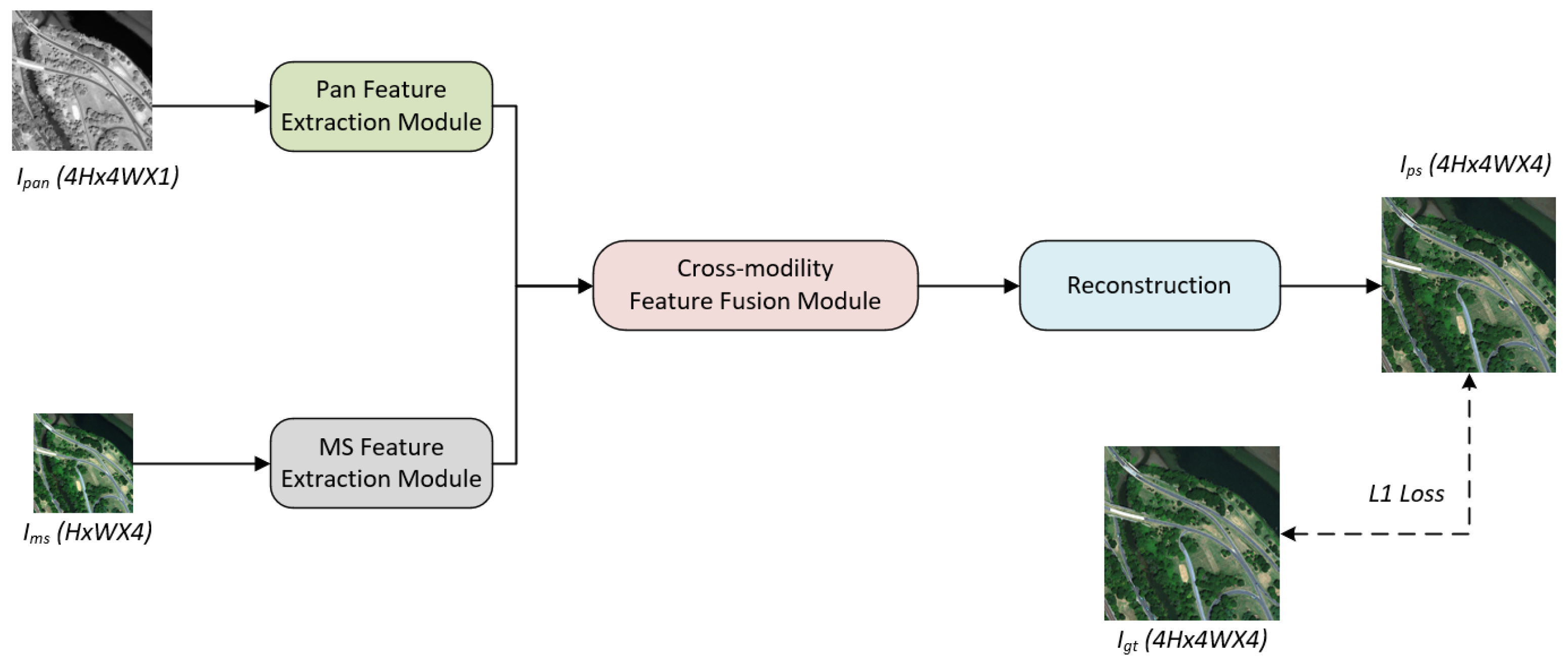
By taking advantage of transformers in computer vision, this paper proposes a dual cross-modality network for pansharpening. Initially, features specific to each modality are extracted from PAN and MS images utilizing Self-Attention Blocks (SABs), and these features are subsequently passed to the Cross-Modality Feature Fusion Module (CMFFM). CMFFM can fuse both spatial and spectral features, effectively integrating relevant and complementary information from the PAN and MS images. Finally, the fused features are sent to the reconstruction module to obtain a pansharpened image. The main contributions of our work can be summarized in three key aspects:

1. We propose two feature extraction modules: the PAN Feature Extraction Module (PFEM) and the MS Feature Extraction Module (MFEM). These modules utilize multiple Self-Attention Blocks (SABs) to extract modality-specific features from PAN and MS images.

2. We present CMFFM that can efficiently combine the cross-modality features of PAN and MS images. CMFFM can improve the incorporation of modality-specific information, improving pansharpening performance.

3. We introduce a network called DCMFN which integrates the modality-specific features. By incorporating details from the fused features, the network improves the complete acquisition of modality-specific information, leading to improved reconstruction results.

The structure of the subsequent sections is presented below. Section 2 provides an overview of the related work, while Section 3 presents a detailed explanation of the proposed DCMFN. Section 4 introduces the relevant experiments, including the dataset, evaluation metrics [10], ablation study, and experimental setup of the SOTA method, and compares them with other SOTA methods in three datasets. The final section provides a summary of the paper.

2. Related Work

Because the pansharpened image has not only a lot of spatial details but also rich spectral information, it is widely used in various object detectors. Current pansharpening methods can be divided into two categories: traditional methods and deep learning-based methods. The characteristics, advantages, and limitations of these methods are summarized in

Table 1. Traditional pansharpening methods.

Method	Characteristics	Advantage	Limitation
CS	Replace the spatial component of the LRMS image with a high-resolution PAN image.	Small computational burden; Significantly enhance the spatial details.	More susceptible to spectral distortion.
MRA	The high-frequency information of the PAN image is injected into the upsampled MS image.	Reduces the risk of spectral distortion.	The fusion effect is sensitive to the detailed injection process.
VO	Transform the image fusion problem into an optimization problem.	Achieve a balance between spatial detail and spectral preservation.	Time-consuming.

and

Table 2. Deep learning-based method for pansharpening.

	Method	Characteristics	Advantage	Limitation
CNN-based	PNN	Bringing CNN to the pansharpening for the first time.	Good detail retention; Strong adaptability.	Limited adaptability to complex scenarios.
	PanNet	The up-sampled MS images propagate spectral information, and the network is trained in a high-pass domain to retain spatial structure.	Enhances the detail of the image.	High data requirements for computing resources
	TFNet	Adopt dual-stream network architecture.	Reduced spectral distortion and loss of spatial detail.	Training and optimization are relatively complex.
	MSDCNN	The convolution matrices of different scales capture multi-scale feature information.	Texture features are richer than single-scale convolution.	Remote sensing images cannot fully utilize the spatial details.
	MUCNN	The convolution kernel converts the spectral information of the panchromatic image into high-frequency details in the spatial domain.	Better performance than direct upsampling.	The processing of extreme bright spots on the image is flawed; Sometimes pixel noise points will appear in solid areas.
	GGPCRN	The interactive connection realizes the collaborative optimization of spectral–spatial features.	Adapt to detail enhancement needs in different scenarios.	Requires high computing resources.
Transformer-based	PanFormer	The cross-modality information of PAN and MS was fused using the cross-attention module.	Performs better than the traditional CNN method on various datasets.	The detail is not rich enough and there is still spectral distortion.
	SSIN	The dual flow network extracts spatial and spectral information respectively, and uses SSA and IIB modules to realize the interaction and fusion of the two kinds of information.	Spatial and spectral information is complementary and interactive.	Sensitive to noise or low-quality data.

in this paper.

Traditional pansharpening methods include Component Substitution (CS) [11], Multi-Resolution Analysis (MRA) [12], and Variational Optimization (VO) [13]. These algorithms have their characteristics: the component replacement method implements spatial information replacement by transform domain processing, the multi-resolution analysis enhances the image by decomposing and injecting spatial details, and the variational optimization utilizes optimization techniques to solve for the best HRMS image. In addition, there are other fusion methods such as the IHS transform and simple average transform.

Traditional pansharpening methods utilize a single pair of LRMS and PAN images to generate a HRMS image at full resolution. However, they often struggle to produce high-quality fused output because they rely on the linear relationship between fused products, which is often flawed [14]. In contrast, deep learning algorithms demonstrate significant potential in image fusion, leveraging their robust nonlinear mapping capabilities, automatic feature learning, and enhanced flexibility and scalability. These advantages are particularly pronounced when working with high-resolution and large-scale datasets.

To mitigate the limitations associated with traditional pansharpening algorithms, a variety of deep learning-based methods have been introduced. For example, CNN is utilized in the field of pansharpening, referred to as PNN [15], which was the first to introduce deep learning into this area. PanNet [16] enhances the black-box aspect of deep learning in PNN by ensuring the preservation of spatial information from both PAN and MS images, while simultaneously retaining the spectral characteristics of the MS data. TFNet [17] performs two-stream input on PAN and MS images to extract features and fuse them into compact feature maps to reconstruct pansharpened images. GGPCRN [18] uses gradient characteristics containing rich structural information to guide the pansharpening process, etc.

The approach mentioned earlier relies on Convolutional Neural Networks (CNNs). However, these CNN-based methods do not take into account the correlation between the PAN and MS bands. Integrating this correlation into the fusion process is essential to mitigate spectral distortion in high-resolution multispectral (HRMS) images. The current research often overlooks the exploration of cross-modality relationships and neglects the enhancement of modality-aware features in pansharpening [19].

With the emergence of the Swin Transformer architecture [20], Zhou et al. introduced self-attention into a two-branch network to extract and merge spectral and spatial features. Subsequently, Nie et al. [21] proposed an innovative network design where attention weights are computed independently from spatial and spectral branches, followed by cross-branch multiplication of attention maps with original feature representations to facilitate mutual information exchange. The effect of these two transformer-based networks is better than that of the CNN-based method, but the feature interaction and fusion of PAN and MS are not sufficient when cross-modality fusion is performed [22]. There is still some degree of spectral distortion and loss of detail [21,22]. To address the above challenges, we propose DCMFN. The network aims to build on the structure of the PanFormer network to further enhance and integrate the correlation and complementary information between PAN and MS images. As a result, our DCMFN produces pansharpened images with less spectral distortion and loss of detail.

3. Proposed Method

3.1. The Overall Architecture of DCMFN

First of all, we begin by detailing the overall architecture of the DCMFN. Following this, we discuss the individual components of the feature extraction modules designed for PAN and MS images, known as PFEM and MFEM. These modules incorporate SAB for effective feature extraction. Next, we provide an overview of the CMFFM, which includes the Successive Swin Transformer Module (SSTM). Finally, we present the reconstruction module.

The architecture of the DCMFN is depicted in Figure 1, which illustrates its overall structure. DCMFN consists of the following three parts.

The first part is the PAN (or MS) Feature Extraction Module. In this module, there are two independent feature extraction modules. We can use these two modules to extract modality-specific features of PAN and MS, respectively. The second part is CMFFM. The modality-specific features extracted from PFEM and MFEM are input into this module. Cross-modality features are generated and fused in this module. By using this module, we can better integrate the two cross-modality features, spatial features, and spectral features. The third part is the reconstruction module. We reconstruct the fusion features into a pansharpened image, which is the pansharpened image we need.

3.2. Feature Extraction Module

In the DCMFN, we introduced the attention mechanism. The attention mechanism addresses the spatial and spectral inconsistencies through spatial attention, spectral attention, and multi-modal fusion. Spatial attention generates feature maps, calculates position-based weights, and can adaptively adjust to deal with spatial differences such as the shift of object positions. Spectral attention extracts spectral features, assigns band-based weights, and resolves spectral variation issues, such as those caused by lighting conditions or sensors. Multi-modality fusion combines spatial and spectral information by leveraging the attention mechanism and adjusts the weights of each type of information according to the task requirements, which is crucial for tasks like object detection and material classification. This comprehensive approach effectively overcomes the challenges posed by the spatial and spectral inconsistencies in the data analysis.

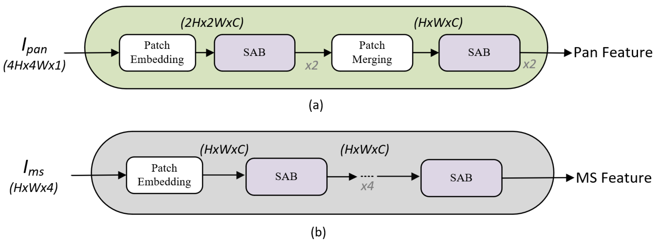
Figure 2a illustrates the proposed framework referred to as the PFEM. Drawing inspiration from Zhou et al. [20], we design the PFEM to incorporate four Self-Attention Blocks (SABs), which is shown in Figure 3. SABs serve as an effective mechanism for feature extraction, particularly for sequential and image data. Each SAB consists of two-layer normalization processes, a self-attention layer, and two multi-layer perceptron (MLP) layers. Figure 3 shows the specific structure of SAB. It computes similarity scores (attention weights) among the elements in the sequence. These scores are then used to take a weighted average of the input features, generating a contextual representation for each position. The calculation is as follows:

$$Att{n}_{self}(Q,K,V)=Softmax\left({\displaystyle \frac{Q{K}^T}{\sqrt{d}}}\right)V$$

(1)

The basic idea is to determine the attention weights by calculating the similarity between the query and the key, and then applying those weights to the value to obtain a weighted output. In both PFEM and MFEM, multiple SABs are used to extract features from the PAN and MS images, respectively. In each SAB, the embedding dimension is set to 64, with 8 attention heads, each having a dimension of 8. The window size is set to 4.

For the MLP layer, the input is first normalized, and the input feature dimension is 64. The feedforward network has an input dimension of 64, a hidden layer dimension of 256, and an output dimension of 64. Finally, a residual connection is applied by adding the input and the output of the feedforward network.

The SAB blocks capture long-range dependencies through a shifted window mechanism. In this mechanism, positional encoding becomes crucial, as it allows the model to maintain spatial awareness while performing attention calculations within local windows. To address this, we introduce the relative indices matrix, which encodes the relative distances between positions within the window. We adjust the positional encoding matrix to avoid negative indexing by adding (W−1) (where (W) is the window size). This ensures that positional encoding can consistently provide effective spatial relationships as the window shifts across the image.

In the case where relative indices are used, the shifting of the attention window can create gaps or cause ambiguity in how distant pixels or patches are spatially related. To resolve this issue, we introduce positional encoding through a learnable embedding matrix. The pos_embedding initializes a 2D positional encoding matrix, which helps the model learn spatial relationships across the image. This matrix, with a size of (7 × 7) for a window size (W = 4), represents relative position embeddings within the attention window, allowing the model to capture spatial information even when working with shifted windows.

The application of multiple SABs in feature extraction offers several advantages. Firstly, these blocks effectively capture long-range dependencies and complex contextual relationships in the data on a layer-by-layer basis. Each Self-Attention Block is capable of addressing varying levels of feature representation, enabling the gradual extraction of more abstract and high-level features. Secondly, each Self-Attention Block is designed to emphasize the correlations among different segments within the sequence. By stacking multiple Self-Attention Blocks, the model can integrate this relevance and contextual information, thereby enhancing its representational capacity regarding the data. Thirdly, stacking multiple Self-Attention Blocks enables the model to address noise and variability more effectively, thereby improving its generalization across diverse data patterns.

Modality-specific features from the PAN and MS images are extracted independently using multiple consecutive SABs. In the feature extraction process for the PAN image, we introduce an additional patch merging layer. This layer is used for combining patches, which enables the transformation of features from size $2H\times 2W\times C$ to match the size $H\times W\times C$ of the MS features for subsequent processing. After extracting these modality-specific features, they are input into the subsequent cross-modality feature extraction module. Further processing occurs within the CMFFM, which is detailed in the following section.

3.3. Cross-Modality Feature Fusion Module (CMFFM)

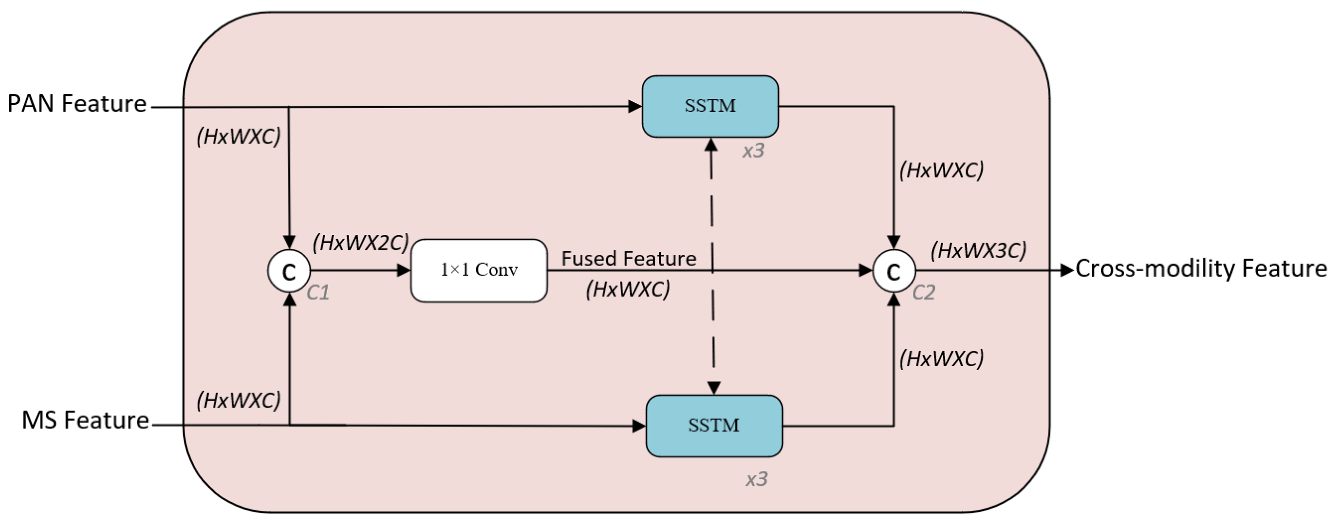
In the previous subsection, we separately extracted the features from the PAN and MS images and inputted them into the CMFFM. This section presents the structure of the CMFFM as illustrated in Figure 4.

First, we feed the modality-specific features ($H\times W\times C$) of PAN and MS into CMFFM as inputs, respectively. Then, the PAN feature and MS feature are concatenated to obtain a fused feature ($H\times W\times 2C$) along the channel dimension. The number of channels is then adjusted to obtain the final fusion feature of size ($H\times W\times C$). At the same time, the PAN feature and MS feature are separately fed into SSTM for further feature extraction. At this point, the size of the new PAN and MS features remains ($H\times W\times C$). Finally, the new PAN and MS features are concatenated with the previous fusion features along the channel dimension to obtain the cross-modality feature as the output of CMFFM.

The main aim of the CMFFM is to utilize the SSTMs to further extract cross-modality features from both PAN and MS images. We leverage fusion features to enhance cross-modality details, thereby improving integration. The direct application of standard transformers, particularly in the computer vision domain, presents several challenges, primarily due to two factors: scale differences and the high resolution of images. The first challenge pertains to scale. In a street scene image, for instance, various objects such as cars and pedestrians differ significantly in size, a phenomenon not present in natural language processing. The second challenge is related to image resolution. When using pixels as the basic unit, the resulting sequence length can become impractically large. To address these issues, researchers have explored various approaches, including partitioning the image into smaller windows and performing self-attention calculations on these windows.

To address the aforementioned challenges, the Swin Transformer network has been introduced [23]. This network employs a sliding window mechanism for feature extraction, which not only enhances computational efficiency but also significantly reduces the sequence length by performing self-attention calculations within the confines of each window. Simultaneously, the shifting operation enables interaction between adjacent windows, fostering cross-window connections across different layers. This design effectively facilitates a form of global modeling while maintaining computational efficiency. To capture the relevant information from PAN and MS images, the approach prioritizes the integration of key features. We incorporate the Swin Transformer and employ the shifting mechanism to facilitate interaction between the information. This leads to the proposal of the structure.

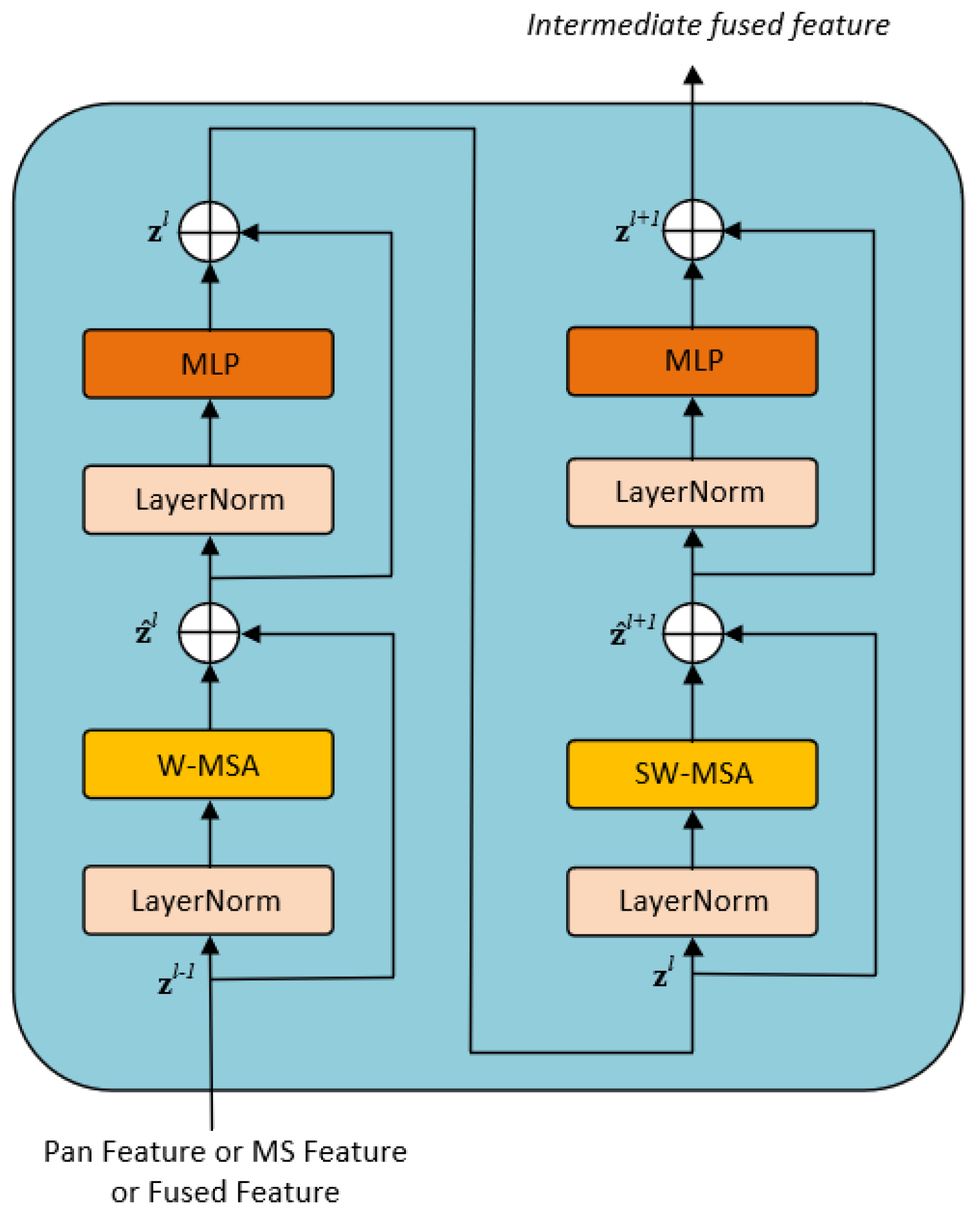
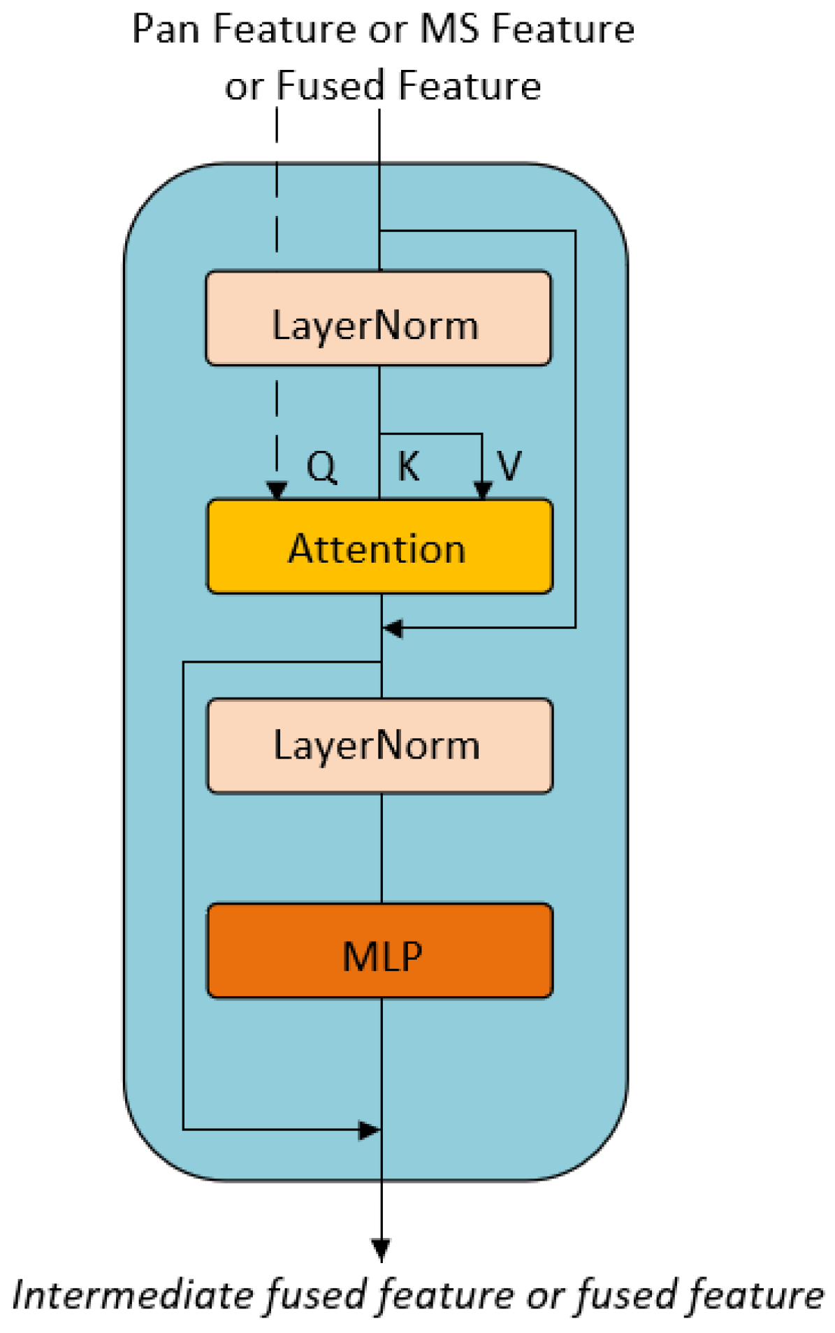
As a key component of the CMFFM, we illustrate the detailed structure of the SSTM in Figure 5. Each SSTM is composed of two consecutive Cross-Attention Blocks (CABs), with the structure of each CAB depicted in Figure 6. The PAN (MS) feature and the fused feature are fed into the CAB as the query (Q) and key–value (K, V) pairs, respectively. This strategy fully capitalizes on the distinct advantages of both MS and PAN, facilitating a more effective utilization of the correlative dependence and complementary information between spatial (spectral) features and their fused counterparts. The attention function CA ($F_a$, $F_b$) can be expressed as

$$CA(F_a,F_b)=Attention(Q\left(F_b\right),K\left(F_a\right),V\left(F_a\right))$$

(2)

Given two features, $F_a$ and $F_b$, the attention mechanism can be employed to model their relationship. CA indicates the relationships between $F_a$ and $F_b$. As defined in Equation (1), the attention function is employed in our application to evaluate CA (·).

In the PFEM and the MFEM, the PAN and MS features are extracted using multiple SABs, resulting in fused features that integrate information from both images. Within the CMFFM, instead of sending the PAN and MS features independently into the SSTM, we input the fused features alongside the MS (or PAN) features. The fused features incorporate the relevance and complementary information between PAN and MS images. Through this incorporation, spatial and spectral information are effectively integrated within the cross-modality fusion features. Consequently, this method enhances spatial resolution by incorporating additional details and reduces spectral distortion commonly associated with using a single spectral source.

3.4. Reconstruction Module

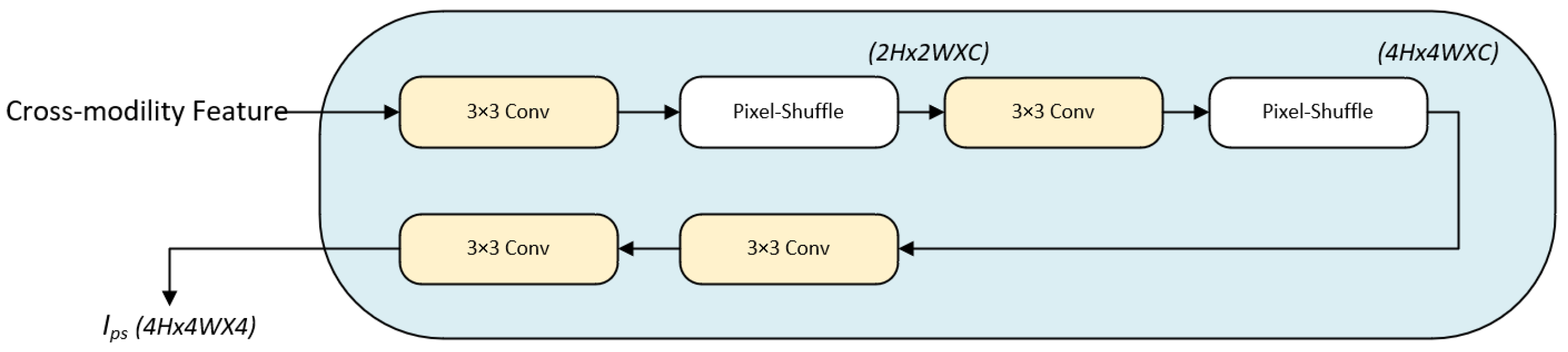
Once the cross-modality fusion features of the image are obtained, they are passed to the reconstruction module as depicted in Figure 7. The size of the input image is $H\times W\times C$. Following several convolution operations and a pixel shuffle, the pansharpened image is generated at this stage, resulting in a size of $4H\times 4W\times 4$.

This module includes several convolutional layers ($conv3\times 3$) and a PixelShuffle operation. Convolutional layers inherently contain learnable parameters (weights and biases), which are optimized during training using backpropagation. In the network architecture, following the second pixel-shuffle operation, the size of the feature transforms into $4H\times 4W\times C$. At this stage, the feature is first directed into the initial $conv3\times 3$ layer. The primary function of this $conv3\times 3$ layer is to extract feature maps across C channels. Subsequently, the final $conv3\times 3$ layer is responsible for generating the ultimate 4-channel fused outcome.

Notably, in Figure 7, two consecutive “$3\times 3$ Conv” blocks are presented at the end. This design is the result of a comprehensive experimental exploration and meticulous design considerations. These two consecutive convolutional blocks play a crucial role in further feature extraction. They can remarkably enhance the network’s capacity to capture detailed features within the input data, thereby effectively improving the overall performance of the network.

Since the convolutional layers contain learnable parameters, the reconstruction module will be updated during training alongside other components of the network. The ReLU activations, which are nonlinear transformations, further ensure the module participates in the training process by introducing nonlinearity.

The PixelShuffle operation itself is a deterministic function used for upsampling, which does not introduce any learnable parameters. However, it works with the convolutional layers that do have learnable parameters, thus participating in the end-to-end optimization of the network.

PixelShuffle is a prevalent image processing technique in deep learning. This technique effectively enhances image resolution by rearranging pixels [23]. Its main role is to convert low-resolution feature maps into high-resolution outputs through pixel rearrangement. This operation is often referred to as spatial rearrangement or pixel arrangement. The advantage of PixelShuffle technology is that it can learn complex image features through deep learning models, enabling the generation of more realistic and detailed high-resolution images. Additionally, since PixelShuffle does not require extra upsampling parameters, such as convolution kernels used in transposed convolution, it enhances the quality of the generated images without increasing the model’s complexity.

4. Experiments

4.1. Datasets

Pansharpening often lacks reference images (Ground Truth, GT) in practical applications, complicating the assessment of the pansharpened image quality. To tackle this issue, Masi et al. introduced an innovative methodology for synthesizing training datasets using the Wald protocol [10]. This methodology generates a dataset encompassing input MS images, PAN images, and HRMS images. The initial PAN and MS images are first processed into blurred versions, employing a modulation transfer function (MTF) kernel for this purpose. After the initial step, the PAN and MS images undergo a reduction in resolution by dividing their pixel dimensions by four. Meanwhile, the original MS image is used as the GT for supervised learning.

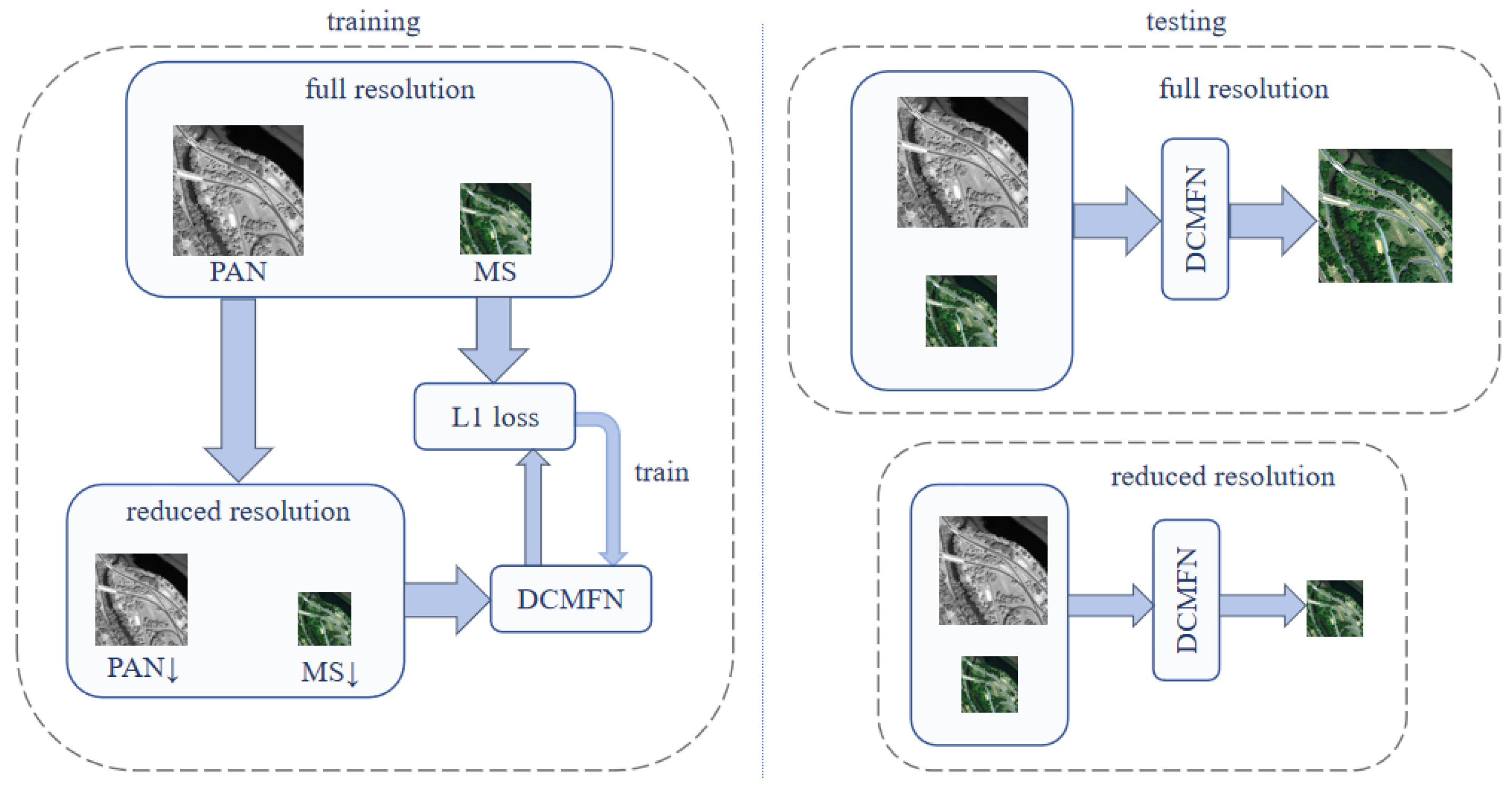
Currently, most pansharpening algorithms that utilize supervised deep learning generate datasets following this methodology. On the one hand, they employ reference image quality evaluation metrics to assess fusion results at a reduced resolution. On the other hand, non-reference image quality metrics are used to evaluate fusion results at full resolution. By considering experimental results at not only full resolution (FR) but also reduced resolution (RR), the quality of fusion images can be assessed more comprehensively.

To clarify the application of RR and FR datasets in training and testing, the flowchart illustrating the training and testing phases using the supervised learning method is presented in Figure 8.

The study presented in [24] offers multiple datasets for pansharpening evaluation. To evaluate the effectiveness of DCMFN, we performed a series of experiments. These experiments were conducted on three urban remote sensing datasets: QuickBird (QB), WorldView-2 (WV2), and WorldView-4 (WV4). The goal was to comprehensively evaluate the performance of the DCMFN across these datasets. These datasets were sourced from commercial satellite systems operated by specialized companies, with a primary focus on urban environments, particularly buildings, while also encompassing other features such as trees and roads [13]. the The datasets used in this study (QuickBird, WorldView-2, WorldView-4) are publicly available for research purposes. They can be accessed through the DigitalGlobe Open Data Program (https://www.digitalglobe.com/).

Detailed information is provided in

Table 3. Details of the three selected datasets.

Satellites	Image Types	Spatial Resolution	Bands	Image Size	Bits
QuickBird	MS	2.88 m	4	$256\times 256\times 4$	11
	PAN	0.72 m	1	$1024\times 1024$
WorldView-2	MS	2 m	8	$256\times 256\times 8$	11
	PAN	0.5 m	1	$1024\times 1024$
WorldView-4	MS	1.24 m	4	$256\times 256\times 4$	11
	PAN	0.31 m	1	$1024\times 1024$

.

He et al. [25] divided the QuickBird (QB) dataset into six categories when used to observe land cover distribution: Class 1: Paddy field; Class 2: Evergreen forest; Class 3: Deciduous forest; Class 4: Cropland; Class 5: Urban area; Class 6: Bare land. These six categories allow for a better understanding of land cover types in different ecological areas, which in turn facilitates research in the following aspects: urban planning (such as analyzing urban structure and infrastructure development through high-resolution images); land use/land cover change (e.g., monitoring and analyzing land changes, assessing deforestation, agricultural expansion, and urbanization); environmental monitoring (e.g., ecosystem health assessment, pollution monitoring, and water pollution analysis); post-disaster assessment (e.g., assessing damage, infrastructure destruction, and more after natural disasters like floods, earthquakes, and fires); and agricultural monitoring (e.g., investigating crop growth, soil conditions, irrigation, and other agricultural factors). As for the Worldview-2 dataset (WV2), Dube et al. mentioned in [26], their study has the potential to combine Worldview-2 data with selected environmental variables to estimate and map above-ground biomass and carbon stocks of managed plantations in a watershed. Therefore, we selected this dataset to study the impact of DCMFN on the ecological environment. Akumu et al. proposed that the use of a high spatial resolution drone and satellite data such as WorldView-4 can provide effective mapping and monitoring in grazing land environments [27]. Therefore, we believe that these three datasets are suitable for the study of pansharpening applications in ecological and environmental monitoring.

Table 3 provides detailed information about the three remote sensing datasets mentioned above. Wald et al. [10] observed that in the experiments involving reduced resolution, the scaled LRMS images had dimensions of 64 × 64. Additionally, the PAN images were scaled to dimensions of 256 × 256. On the other hand, the dimensions were 256 × 256 for LRMS and 1024 × 1024 for PAN in the full-resolution experiments.

For each dataset, the data are randomly divided into a training set and a test set: 80% is assigned to the training set, 20% to the test set, with 20% further used as a validation set. To mitigate the challenges posed by limited data, we implemented data augmentation techniques, which encompassed random cropping, horizontal flipping, and rotation. As a result, the training samples consisted of 400 images for QB, 2380 images for WV4, and 400 images for WV2.

In the validation phase, to evaluate the performance of the network, we used 80 pairs of images for both the first two datasets, and 76 pairs for the third dataset.

4.2. Evaluation Indexes

In our study, we evaluated the above 3 datasets in both RR and FR tests. In the RR evaluation, we employed several performance metrics, including the Spectral Angle Mapper (SAM) [24], the Erreur Relative Globale Adimensionnelle de Synthèse (ERGAS) [28], the Correlation Coefficient (CC) [29], and the Extended Universal Image Quality Index (Q2n, with Q4 and Q8 for four-band and eight-band images, respectively) [30].

We computed three additional metrics: the Spatial Correlation Coefficient (SCC), the Spatial Distortion Index $D_S$, and the Spectral Distortion Index $D_{\lambda }^K$. Furthermore, the High-Quality No Reference (HQNR) metric was also utilized. According to Yusupov et al. [31], the value of HQNR can be obtained using $D_S$ and $D_{\lambda }^K$. In other words, HQNR helps us evaluate the quality of images by measuring spatial and spectral distortions. The spatial distortion is related to the spatial component ($D_S$) of the image, and the spatial distortion represents the degree of distortion of features such as pixel change, texture, and edge in the image. Related to the spectral component of the image ($D_{\lambda }^K$), spectral distortion represents the distortion of the image in the frequency domain, usually affecting the high-frequency portion of the image. The mean absolute difference of the $D_{AVE}$ values across all channels is used to obtain the value of $D_S$ (the $D_{AVE}$ calculation method and practical significance are also described in the paper). The spectral distortion index $D_{\lambda }^K$ is found according to Khan’s protocol [32]. The lower $D_{\lambda }$, $D_S$, and the higher QNR correspond to the better image quality [33].

4.3. Training Details

To ensure stable training conditions, the AdamW [34] optimizer optimizer is utilized, and the learning rate is $5\times {10}^{-4}$. Our network, DCMFN, is based on the Transformer architecture. It follows the training strategy described in [12]. And this architecture does not undergo any pre-training. The initial learning rate is set to 0.0005 and is gradually reduced to 0.00005 over a duration of 1200 epochs, using a cosine annealing schedule as the training progresses. Additionally, the batch size is set to 10, and the hidden channel C is configured to 64. The window size is 4 in both SABs and CABs, with every attention mechanism comprising 8 heads. The loss training is calculated using the L1 norm. The calculation of the loss is

$$L=\sum _{n=1}^N{\parallel I_{ps}^{\left(n\right)}-I_{gt}^{\left(n\right)}\parallel }_1$$

(3)

Utilizing a GTX-1080Ti GPU with PyTorch 1.7.1, the deep learning methods are implemented, and the results for all methodologies are calculated using MATLAB R2019b. Furthermore, the average values reported correspond to the respective test datasets.

4.4. Ablation Study

In the ablation study, we conducted an array of experimental evaluations on the WV4 dataset to assess the effectiveness of the CMFFM. In each table, the best values are in bold, the second-best values are underlined. The downward arrow (↓) denotes a preference for a lower value, while the upward arrow (↑) signifies a preference for a higher value [22]. used for preprints.

4.4.1. The Effects of the Features Fused in the CMFFM

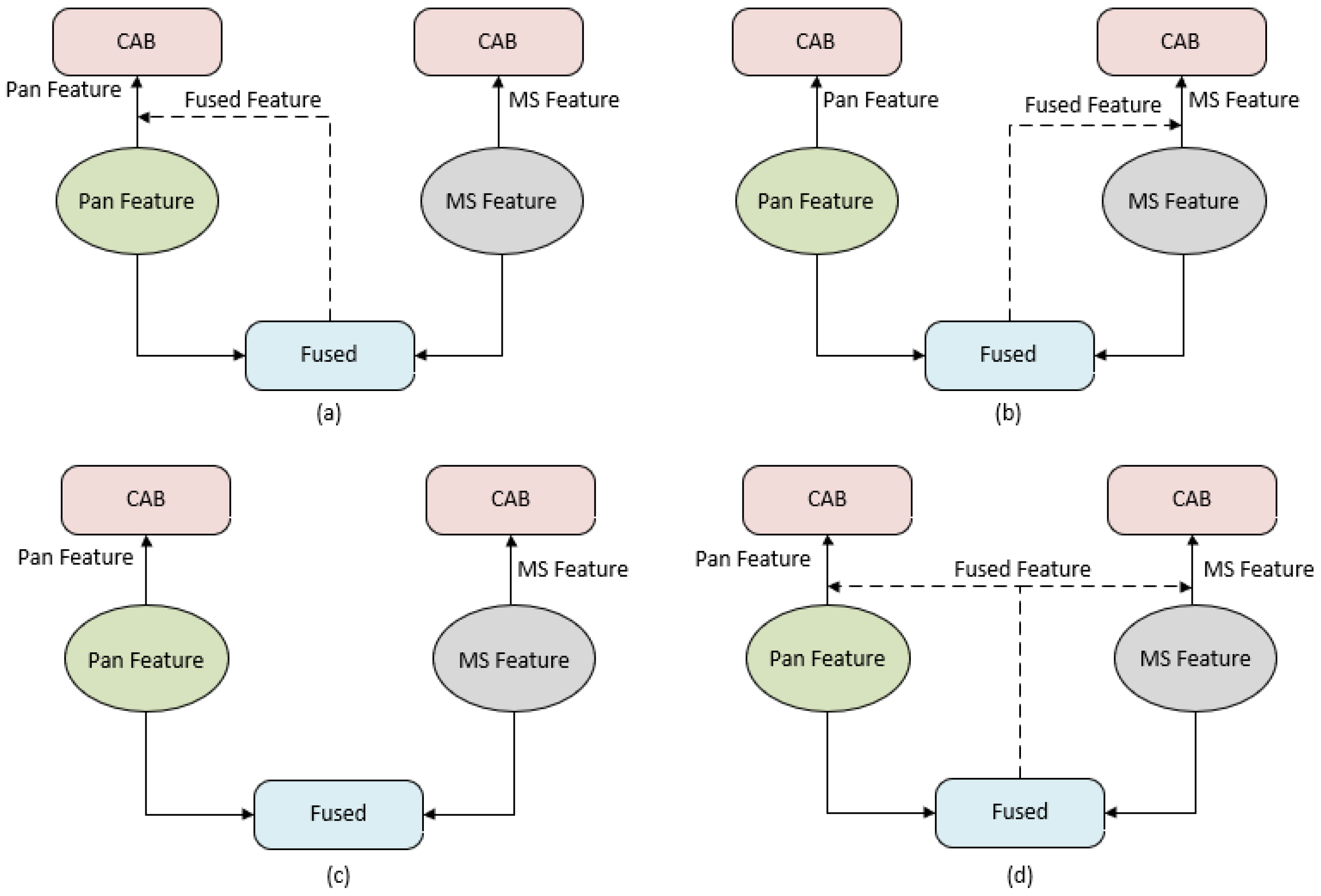
The Cross-Modality Feature Fusion Module (CMFFM) is crucial for pansharpening. As a result, our ablation study evaluates various implementations of CMFFM within the Dual Cross-Modality Fusion Network (DCMFN). The detailed architectures are illustrated in Figure 9, showcasing four different methods for fusing a pair of features:

• PAN-Fused and MS (P-F & M)
  As illustrated in Figure 9a, the first method involves concatenating the PAN feature with the fused feature. This approach allows details from the features of the PAN to be added to the fused features. Meanwhile, the MS features are directly input into the CAB module without concatenation with the fused features. The computation can be expressed as follows:

  $$F_1=[CA(F_{PAN},F_{Fused});CA\left(F_{MS}\right)]$$

  (4)
• PAN and MS-Fused (P & M-F)
  As is shown in Figure 9b, the second implementation involves concatenating the MS feature with the fused feature. In this implementation, the fused feature is integrated alongside the MS feature to improve the richness of the detailed information. Conversely, the PAN features are directly input into the CAB module without concatenation with the fused features. The computation can be expressed as follows:

  $$F_2=[CA\left(F_{PAN}\right);CA(F_{MS},F_{Fused})]$$

  (5)
• PAN-MS and PAN-MS (P-M & P-M)
  As illustrated in Figure 9c, the modality features are extracted not only from MS but also from PAN through concatenation, facilitating the subsequent integration of these cross-modality features into the reconstruction image. The calculation is

  $$F_3=[CA(F_{PAN},F_{MS});CA(F_{MS},F_{PAN})]$$

  (6)
• PAN-Fused and MS-Fused (P-F & M-F) (ours)
  As depicted in Figure 9d, the modality features of MS and PAN are derived by integrating the PAN feature and MS feature with the fused feature. This approach facilitates the subsequent fusion of these two cross-modality features into the reconstruction image. The calculation is

  $$F_4=[CA(F_{PAN},F_{Fused});CA(F_{MS},F_{Fused})]$$

  (7)

The results of the four architectures are presented in

Table 4. Quantitative results from the ablation studies are presented as follows. This table shows the results of various metrics from the ablation studies, with performance comparisons across different configurations. The best results are highlighted in bold.

Modules	P-F & M	P & M-F	P-M & P-M	P-F & M-F (Ours)
SAM↓	$\underline{1.4716}$	$1.5907$	$1.6050$	$\mathbf{1}.\mathbf{4240}$
ERGAS↓	$\underline{1.3011}$	$1.5063$	$1.5103$	$\mathbf{1}.\mathbf{2587}$
Q2N↑	$\underline{0.8900}$	$0.8782$	$0.8751$	$\mathbf{0}.\mathbf{8924}$
CC↑	$\underline{0.9789}$	$0.9737$	$0.9736$	$\mathbf{0}.\mathbf{9901}$
${\mathbf{D}}_{\mathbf{\lambda }}^{\mathbf{K}}$↓	$\underline{0.0789}$	$0.0806$	$0.0931$	$\mathbf{0}.\mathbf{0786}$
${\mathbf{D}}_{\mathbf{S}}$↓	$0.0535$	$\mathbf{0}.\mathbf{0449}$	$0.0636$	$\underline{0.0529}$
HQNR↑	$\underline{0.8713}$	$0.8712$	$0.8492$	$\mathbf{0}.\mathbf{8727}$

. In Table 4 and

Table 5. Quantitative results from the ablation studies are presented as follows. This table presents the quantitative results of the ablation studies, including the performance metrics for different modules.

Modules	Without, C1+C2	C1	C2	Parallel, C1+C2
SAM↓	1.6050	1.5244	1.4701	1.4240
ERGAS↓	1.5103	1.3793	1.3045	1.2587
$\mathbf{Q}{\mathbf{2}}^{\mathbf{n}}$↑	0.8751	0.8845	0.8892	0.8924
CC↑	0.9736	0.9770	0.9788	0.9901
${\mathbf{D}}_{\mathbf{\lambda }}^{\mathbf{K}}$↓	0.0931	0.0731	0.0715	0.0706
${\mathbf{D}}_{\mathbf{S}}$↓	0.0636	0.0537	0.0537	0.0529
HQNR↑	0.8492	0.8721	0.8726	0.8727

, we just show the average values at first to keep it simple. We perform statistical analyses like t-tests and F-tests to check the significance of differences between groups. The p-values are below 0.05, so the results are statistically significant. Both the PAN-Fused and MS, and MS-Fused and PAN approaches enhance the performance relative to the basic concatenation baseline, whose structure is shown in Figure 9c. However, the performance of the PAN and MS-Fused strategy is comparatively lower. In addition to $D_S$, the best results are achieved by integrating these two strategies of cross-attention, which we designate as DCMFN.

In the cross-attention model, the results demonstrate that information exchange among different modalities plays a significant role in producing enhanced fusion representations, which implies that the CMFFM significantly enhances the overall effectiveness.

4.4.2. The Effects of the Concatenation in the CMFFM

Figure 4 illustrates the structure of the CMFFM, which incorporates two concatenations, C1 and C2. C1 represents the feature map after the concatenation of PAN and MS features on the channel ($H\times W\times 2C$); C2 represents the Cross-modality Feature ($H\times W\times 3C$) obtained after passing through our CMFFM. The effectiveness of these concatenations was evaluated separately on the WV4 dataset, with results presented in Table 5. The performance metrics indicate that utilizing either concatenation C1 or C2 yields improvements over the method that excludes both. However, the optimal pansharpening results are achieved when both C1 and C2 are employed simultaneously within the network.

5. Comparisons with SOTA Methods

To assess the performance of DCMFN, we conduct evaluations using data from various satellites. We select five traditional methods for comparison: EXP [35], BDSD-PC [36], GSA [37], PRACS [38], and MTF-GLP [35]. The implementations of these traditional methods utilized in this study are available from [28]. We select eight DL-based methods, including PNN [15], PanNet [16], MSDCNN [39], TFNET [17], GGPCRN [18], MUCNN [40], PanFormer [20], and SSIN [21]. Each of these methods represents a significant contribution to the pansharpening field, and their inclusion allows us to benchmark DCMFN against the latest advances in deep learning in the task at hand. We perform statistical analyses like t-tests and F-tests to check the significance of differences between groups. The p-values are below 0.05, so the results are statistically significant. For the competing methods, we use the same experimental parameters as those for DCMFN, including the training learning rate, optimizer, loss function for training, the computer devices used for training, and so on. In this paper, all the deep learning-based competing methods were trained from scratch on the same dataset used for DCMFN.

5.1. Experiments on Reduced-Resolution Datasets

For the QB dataset,

Table 6. Quantitative results of different methods at reduced resolution for the QB dataset.

Methods	SAM ↓	ERGAS ↓	Q2N ↑	CC ↑
EXP	$1.8769$	$1.8077$	$0.6922$	$0.8351$
BDSD-PC	$0.8769$	$0.7548$	$0.9483$	$0.9662$
GSA	$0.8582$	$0.7634$	$0.9461$	$0.9664$
PRACS	$0.9005$	$0.8011$	$0.9394$	$0.9657$
MTF-GLP	$0.8307$	$0.7308$	$0.9498$	$0.9686$
PNN	$0.9998$	$0.9341$	$0.8663$	$0.9610$
PanNet	$0.9990$	$0.7754$	$0.8874$	$0.9703$
MSDCNN	$0.9978$	$0.7711$	$0.8833$	$0.9696$
TFNET	$0.7951$	$0.6037$	$\underline{0.9090}$	$0.9810$
GGPCRN	$0.7993$	$0.6021$	$0.8925$	$0.9830$
MUCNN	$0.9239$	$0.7207$	$0.8935$	$0.9732$
PanFormer	$0.8483$	$0.6441$	$0.8996$	$0.9776$
SSIN	$0.7136$	$0.6020$	$0.9067$	$0.9845$
DCMFN (ours)	$\mathbf{0}.\mathbf{7033}$	$\mathbf{0}.\mathbf{6011}$	$\mathbf{0}.\mathbf{9294}$	$\mathbf{0}.\mathbf{9992}$

presents the quantitative evaluation performance results. These results indicate that DCMFN achieves the highest ranking across all metrics, closely followed by SSIN. This is despite the fact that our method ranks second in the Structural Similarity Measure (SAM). It is notable that the difference between our results and the best performance by SSIN is minimal, differing only by a fraction of a decimal point. For the remaining two datasets, WV2 and WV4, the quantitative evaluation performance results are presented in

Table 7. Quantitative results of different methods at reduced resolution for the WV2 dataset.

Methods	SAM ↓	ERGAS ↓	Q2N ↑	CC ↑
EXP	7.5665	10.4587	0.6677	0.7925
BDSD-PC	5.9096	5.8233	0.7138	0.9427
GSA	6.0134	6.2266	0.7017	0.9324
PRACS	6.6875	6.8691	0.7797	0.9282
MTF-GLP	5.9651	6.1457	0.7027	0.9347
PNN	3.7474	3.4182	0.7464	0.9539
PanNet	3.5791	3.1939	0.7546	0.9593
MSDCNN	3.4938	3.0776	0.7549	0.9612
TFNET	3.0540	2.5875	0.7685	0.9714
GGPCRN	2.9430	2.4572	0.7741	0.9743
MUCNN	3.2474	2.8515	0.7588	0.9661
PanFormer	3.1938	2.8036	0.7596	0.9666
SSIN	2.9114	2.4036	0.7757	0.9752
DCMFN (ours)	2.8799	2.3422	0.7866	0.9810

and

Table 8. Quantitative results of different methods at reduced resolution for the WV4 dataset.

Methods	SAM ↓	ERGAS ↓	Q2N ↑	CC ↑
EXP	2.1106	1.9301	0.7611	0.9640
BDSD-PC	2.1545	1.2828	0.8802	0.9827
GSA	1.7325	1.2715	0.8779	0.9821
PRACS	1.9273	1.3257	0.8793	0.9831
MTF-GLP	1.7301	1.2954	0.8765	0.9818
PNN	1.9462	1.9320	0.8364	0.9595
PanNet	1.8639	1.8076	0.8483	0.9637
MSDCNN	1.8139	1.7549	0.8561	0.9652
TFNET	1.4770	1.2671	0.8981	0.9815
GGPCRN	1.5211	1.3458	0.9079	0.9849
MUCNN	1.6931	1.3561	0.8742	0.9697
PanFormer	1.6050	1.5103	0.8751	0.9736
SSIN	1.4803	1.3238	0.8911	0.9858
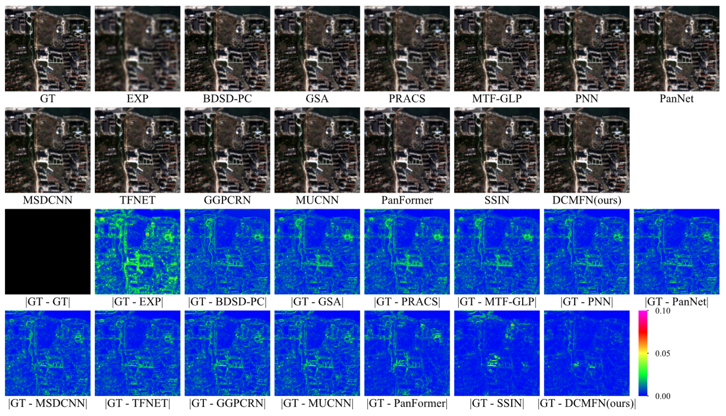
DCMFN (ours)	1.4240	1.2587	0.8924	0.9901

, where DCMFN consistently outperforms all indicators on the WV4 dataset, particularly excelling in the SAM and ERGAS metrics. In addition to the quantitative assessments, this experiment also compares the subjective visual results. It offers a comprehensive evaluation of the effectiveness of different methods across the three different datasets mentioned above. In order to highlight the abilities of DCMFN in maintaining spectral integrity and enhancing detail, images with rich detail and spectral characteristics are specifically selected for visual examination. 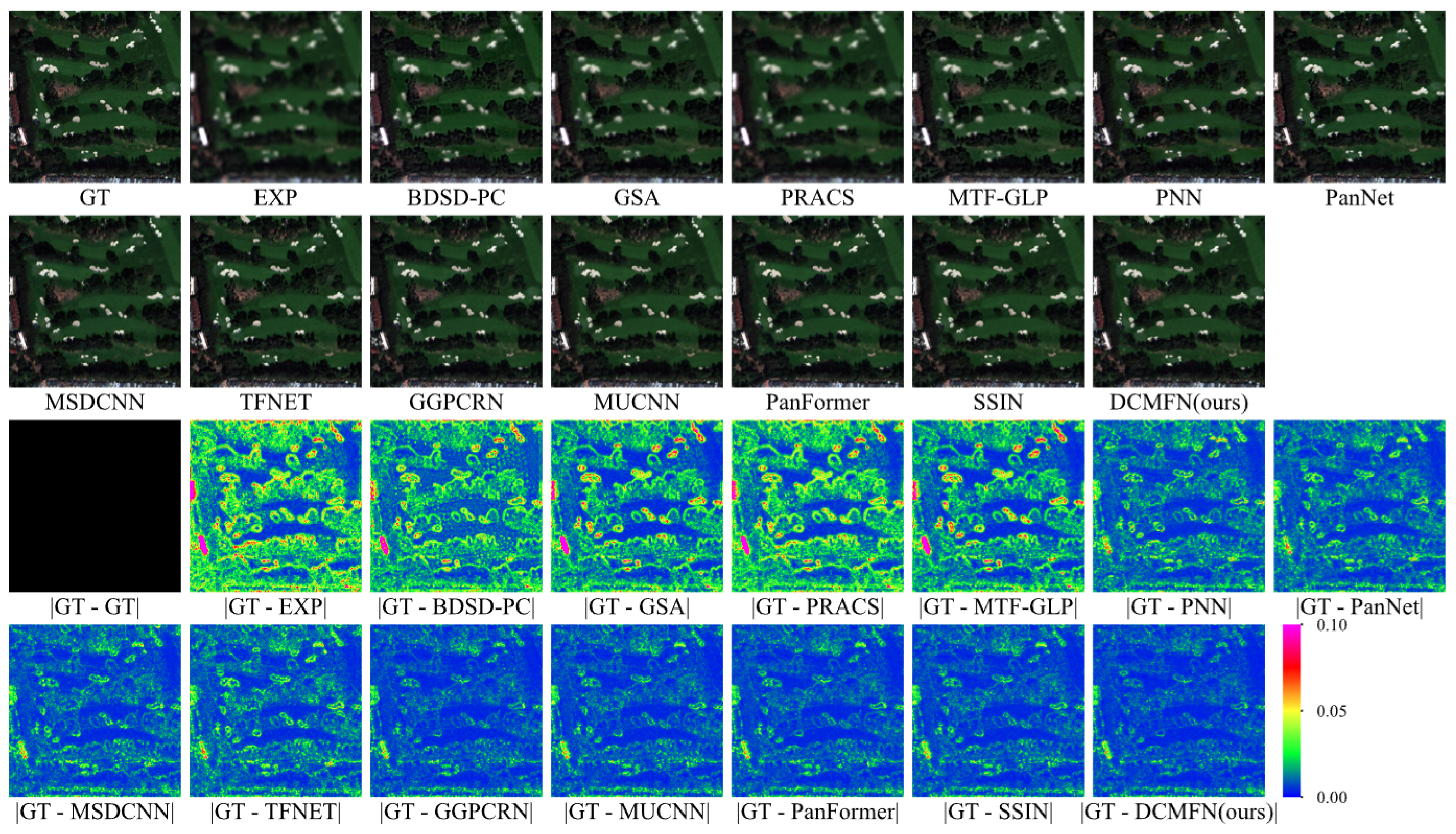The visual results from different methods are showcased in Figure 10, Figure 11 and Figure 12, featuring random selections from the three datasets. The first two rows exhibit RGB images. Conversely, the next two rows depict images that result from averaging the residuals across different bands.

Figure 10 illustrates, for the QB dataset, traditional methods, such as EXP, BDSD-PC, and PRACS. Fuzzy results are produced when the residuals of each band are averaged, particularly with EXP and PRACS, which inject little to no detail. Although these traditional methods generate pansharpened images, they lack sufficient detail in contrast to the ground truth (GT). In contrast, the eight deep-learning-based methods produce vivid and clear results, effectively capturing intricate details. The analysis of the residual images indicates that the performance of DCMFN closely aligns with that of GT, demonstrating that DCMFN exhibits superior capabilities in both detail recovery and spectral fidelity.

Figure 11 presents similar findings. The results achieved by all methods on the WV2 dataset are marginally lower in quality compared to those observed with the QB dataset, which we hypothesize is due to the WV2 dataset containing twice as many bands as the QB dataset. Furthermore, aside from DCMFN, other deep learning-based methods exhibit different levels of spectral distortion, which is shown by the white roof located in the lower left corner of the image.

Figure 12 presents the results for the WV4 dataset. Analysis of the residual images indicates that deep learning (DL) methods outperform others, highlighting the superior panchromatic sharpening capabilities of DL approaches. In Figure 10, the ground truth (GT) image reveals a greater number of scattered white roofs. As shown in the subsequent residual images, traditional methods exhibit suboptimal panchromatic sharpening effects for these white roofs, whereas our proposed DCMFN demonstrates the most effective performance. Additionally, our DCMFN achieves the most effective panchromatic sharpening results for this dataset.

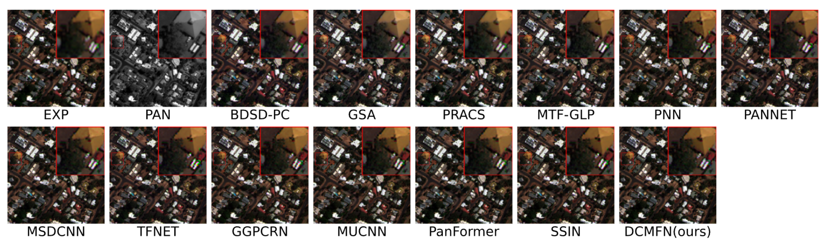
5.2. Experiments on Full-Resolution Datasets

To assess the generalization capabilities of the discussed methods, extensive experiments were conducted at full resolution. Quantitative results for the above three datasets are presented in

Table 9. Quantitative results of different methods at full resolution for the QB dataset.

Methods	${\mathit{D}}_{\mathit{\lambda }}^{\mathit{K}}$↓	${\mathbf{D}}_{\mathbf{S}}$↓	HQNR↑
EXP	$0.0510$	$0.1016$	$0.7648$
GSA	$0.1269$	$0.1743$	$0.7287$
PRACS	$0.0836$	$0.1096$	$0.8197$
MTF-GLP	$0.0694$	$0.2004$	$0.7483$
PNN	$0.0999$	$0.1201$	$0.1975$
PanNet	$0.0635$	$0.9070$	$0.8542$
MSDCNN	$0.0946$	$0.1012$	$0.8192$
TFNET	$\underline{0.0474}$	$\underline{0.0591}$	$\underline{0.8975}$
GGPCRN	$0.0528$	$0.0608$	$0.8911$
MUCNN	$0.0946$	$0.1012$	$0.8192$
PanFormer	$0.0802$	$0.0610$	$0.8655$
SSIN	$0.0477$	$0.0646$	$0.8918$
DCMFN (ours)	$\mathbf{0}.\mathbf{0242}$	$\mathbf{0}.\mathbf{0357}$	$\mathbf{0}.\mathbf{9410}$

,

Table 10. Quantitative results of different methods at full resolution for the WV2 dataset.

Methods	${\mathit{D}}_{\mathit{\lambda }}^{\mathit{K}}$↓	${\mathbf{D}}_{\mathbf{S}}$↓	HQNR↑
EXP	0.1970	0.1052	0.7089
BDSD-PC	0.2478	0.1428	0.6586
GSA	0.1988	0.1690	0.6811
PRACS	0.1294	0.0958	0.7944
MTF-GLP	0.0932	0.1762	0.7567
PNN	0.2788	0.0979	0.6565
PanNet	0.2072	0.1008	0.7180
MSDCNN	0.2215	0.1044	0.7042
TFNET	0.1918	0.1041	0.7294
GGPCRN	0.1800	0.0983	0.7455
MUCNN	0.2352	0.1188	0.6857
PanFormer	0.2771	0.0974	0.6611
SSIN	0.1696	0.0894	0.7573
DCMFN (ours)	0.0824	0.0952	0.8302

and

Table 11. Quantitative results of different methods at full resolution for the WV4 dataset.

Methods	${\mathit{D}}_{\mathit{\lambda }}^{\mathit{K}}$↓	${\mathbf{D}}_{\mathbf{S}}$↓	HQNR↑
EXP	$0.0800$	$0.0819$	$0.8479$
BDSD-PC	$0.1567$	$0.1258$	$0.7407$
GSA	$0.2097$	$0.1576$	$0.6700$
PRACS	$0.1233$	$0.0975$	$0.7930$
MTF-GLP	$\underline{0.0821}$	$0.1332$	$0.7984$
PNN	$0.1090$	$0.0591$	$0.8496$
PanNet	$0.0911$	$0.0560$	$0.0859$
MSDCNN	$0.1007$	$0.0534$	$0.8544$
TFNET	$0.0965$	$0.0545$	$0.8558$
GGPCRN	$0.0974$	$0.0563$	$0.8527$
MUCNN	$0.0963$	$0.5470$	$0.8564$
PanFormer	$0.1121$	$0.0542$	$0.8512$
SSIN	$0.0890$	$0.0533$	$0.8634$
DCMFN (ours)	$\mathbf{0}.\mathbf{0786}$	$\mathbf{0}.\mathbf{0529}$	$\mathbf{0}.\mathbf{8727}$

, respectively. It is essential to highlight that the EXP method, which upscales LRMS images without adding detail, is excluded from this comparison. The results across the three datasets indicate that except $D_S$ on the QB dataset is the second best, our proposed DCMFN method ultimately surpasses all other methods across all evaluation metrics, with SSIN following closely behind. Notably, the $D_{\lambda }$ and $D_S$ metrics for the QB dataset are significantly higher than other deep learning-based methods. Similarly, on WV2 and WV4 datasets, $D_{\lambda }$ also shows substantial improvements over the other methods.

Figure 13, Figure 14 and Figure 15 show the FR visual results of all methods for three datasets, featuring random selections from the three datasets. Quantitative results for the three datasets are provided separately. It is obvious that the EXP method, which upscales low-resolution multispectral (LRMS) images without adding detail, is excluded from this comparison. The results across the three datasets indicate that except $D_S$ on the QB dataset is the second best, DCMFN method ultimately surpasses all other methods across all evaluation metrics, with SSIN following closely behind. Notably, the $D_{\lambda }$ and $D_S$ metrics for the QB dataset are significantly higher than other deep learning-based methods. Similarly, on the WV2 and WV4 datasets, $D_{\lambda }$ also shows substantial improvements over the other methods. 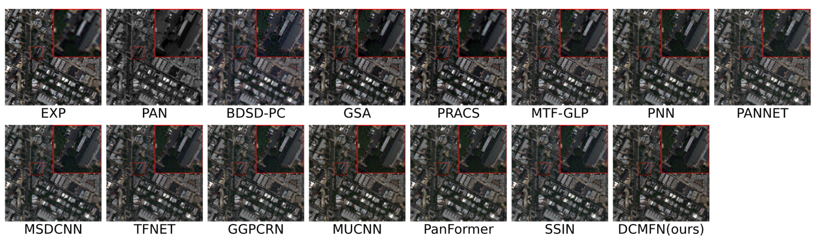Furthermore, the full-resolution visualization results of various methods are conducted across the three datasets as illustrated in Figure 13, Figure 14 and Figure 15. 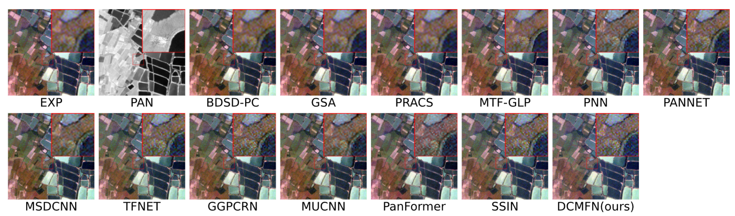In Figure 13, it is evident that deep learning-based methods, including PNN, PANNET, and particularly TFNET and GGPCRN, exhibit significant spectral distortion in the magnified regions of the image. The traditional pansharpening method yields average visual results, often resulting in blurry output. In contrast, DCMFN delivers the best visual quality, showcasing a more vivid image, particularly excelling in edge recovery, such as that of the stones, with higher clarity and reduced spectral distortion.

In Figure 14, the enlarged area reveals that the results from traditional methods exhibit poor panchromatic sharpening effects, resulting in images that lack vibrancy and display significant spectral distortion. Conversely, most deep learning-based methods yield improved results; however, the local magnified section highlights a specific spectral distortion in all methods except for DCMFN, particularly noticeable in the middle rectangular light gray roof. Additionally, in the lower left corner, the dark gray roof shows edge distortion in many methods, whereas DCMFN demonstrates relatively minimal distortion in this region.

In Figure 15, similar to Figure 14, the traditional method yields unsatisfactory results, while the deep learning-based methods produce more vibrant panchromatic sharpening outcomes. Among these, the white roof in the lower right corner of the magnified area exhibits significant spectral distortion, with DCMFN showing reduced distortion compared to other methods. Additionally, the edge of the yellow roof in the same area displays serious distortion in all methods except for DCMFN and MSDCNN.

In conclusion, the experimental results from three urban remote sensing datasets, encompassing both RR and FR data, demonstrate that our DCMFN effectively balances spectral and spatial fidelity.

In

Table 12. Inference time and parameters of deep learning-based models.

Model	#Params	Times
PNN	0.080 M	0.0012
PanNet	0.078 M	0.0032
MSDCNN	0.262 M	0.0035
TFNET	2.359 M	0.0095
GGPCRN	1.771 M	0.014
MUCNN	1.36 M	0.0080
PanFormer	1.530 M	0.0468
SSIN	3.36 M	0.0157
DCMFN	1.710 M	0.0512

, we present the inference time and the scale of models based on deep learning. Specifically, we provide the average time cost for each image within the WorldView3 testing set. For models relying on Generative Adversarial Networks (GANs), we only take into account the parameters within the generator. As shown in Table 12, the number of parameters in our method is comparable to that of PanFormer and GGPCRN. However, our method consumes more time compared to CNN-based approaches. The reason lies in the fact that calculating attention requires more time than performing convolution operations.

6. Discussion

In this paper, we examine the importance and potential benefits of combining pansharpening technology with remote sensing imagery within the realms of ecological and environmental monitoring. The DCMFN method introduced herein has shown superior performance compared to existing deep learning approaches, as evidenced by ablation studies and comparative analyses conducted on three distinct datasets, which are shown in Table 6, Table 7, Table 8, Table 9, Table 10 and Table 11.

Our model is designed to surmount several pivotal challenges in ecological monitoring. First and foremost, the satellite imagery prevalently employed in ecological research often has limited spatial resolution. In ecological investigations, high-resolution data play an irreplaceable role in accurately discerning and charting diverse ecological elements. For instance, they are essential for pinpointing individual plant species, delineating small-scale habitats, and identifying wildlife corridors. The pansharpening techniques integrated into our model serve to augment the spatial details within multispectral images. This augmentation enables us to monitor these ecological features with far greater precision, facilitating more in-depth ecological studies. Another formidable challenge stems from the intricate and ever-changing nature of ecological systems. Ecological variables are in a constant state of flux over time. Traditional monitoring approaches frequently struggle with capturing these rapid and often subtle shifts. However, our model, equipped with the ability to promptly process and analyze pansharpened data, demonstrates remarkable sensitivity in detecting minute changes in aspects such as vegetation vitality, water quality, and land cover. This capability is invaluable for the early detection of ecological disruptions. Whether it is the encroachment of invasive species, the onset of deforestation, or the degradation of wetlands, our model can sound the alarm at an early stage, enabling timely intervention.In addition, the cost effectiveness of ecological monitoring is a critical consideration, particularly for large-scale monitoring initiatives. The acquisition of high-resolution imagery typically incurs substantial costs. Our model offers a more economically viable solution by leveraging pansharpening to enhance the quality of existing lower-resolution data. In doing so, it extracts the maximum value from the available data resources. This not only reduces the need for frequent and costly high-resolution satellite data acquisitions but also ensures that the requisite level of detail for effective ecological monitoring is maintained. By striking this balance, our model makes significant contributions to the sustainable development of ecological monitoring efforts.

Nevertheless, in Figure 10, Figure 11, Figure 12, Figure 13, Figure 14 and Figure 15, we can see that in both RR and FR, although the performance of our DCMFN is excellent, there is still room for improvement. For example, in our experiments, we observe that the DCMFN method struggles under specific conditions. In complex scenes such as highly urbanized areas with numerous high-rises and intricate road networks, the method fails to fully capture and reconstruct details, leading to blurry pansharpening results. When dealing with low-SNR input data, the method has difficulty differentiating real details from noise, causing inaccurate sharpening and introducing artifacts.

Pansharpening significantly boosts the resolution of remote sensing images, allowing for a more accurate depiction of subtle changes on Earth’s surface. This enhanced capability is vital for detecting natural phenomena or environmental alterations. By augmenting remote sensing images with detailed information, pansharpening highlights subtle variations in factors such as land use, vegetation dynamics, water contamination, and air quality. These detailed observations are crucial for understanding environmental changes and their impact on ecosystems. For example, researchers can employ high-resolution remote sensing data to monitor the dispersion of pollutants through water, air, and soil, thereby gaining insights into their behavior in natural settings. Such precise observations assist in evaluating the potential risks of environmental pollutants to ecosystems, flora, fauna, and their persistence and toxic effects. Advancements in remote sensing technology, when paired with pansharpening, enable the integration of various spectral bands, thereby improving both spatial and spectral resolution. This allows researchers to analyze environmental changes from both broad and fine-scale perspectives. In studying pollutant diffusion in the atmosphere, high-resolution remote sensing data can capture the spatial distribution, concentration shifts, and interactions with other pollutants. This provides a solid scientific foundation for environmental pollution control strategies.

In the context of ecological and environmental monitoring, pansharpening technology provides enriched geographical background data, aiding in the optimization of environmental management strategies. By examining regional environmental characteristics via remote sensing images, researchers can more accurately predict environmental trends under specific conditions.

Additionally, the utilization of pansharpening technology, especially with high-resolution remote sensing data, promotes interdisciplinary collaboration. It bridges fields such as environmental science, geography, and ecology, enabling scientists to gather comprehensive environmental information through remote sensing. When combined with in-depth environmental research, this integration explores the effects of environmental changes on Earth’s ecosystems and their practical applications. This not only fosters innovation in environmental monitoring but also offers valuable scientific data and decision-making support for global environmental protection, public health, and resource management.

7. Conclusions

In this study, we proposed a network called DCMFN that employs an attention mechanism for pansharpening. The network first uses two independent extraction modules, PFEM and MFEM, to obtain the spatial and spectral features of the image respectively, and then uses CMFFM to achieve the fusion of the above cross-modality features, which enhances the spectral and spatial details of the image. Finally, the rich fusion features are reconstructed into the pansharpened image. Extensive experiments were conducted using QB, WV2, and WV4 remote sensing datasets. This paper provides a detailed comparison of objective performance indicators and subjective visual results, demonstrating the effectiveness of DCMFN in improving the quality of urban remote sensing images.

Integrating pansharpening technology with remote sensing images provides rich, accurate data for environmental monitoring. This combination holds significant potential for advancing research in ecological and environmental monitoring, particularly in tracking changes in ecosystems, land use, and natural phenomena. High-resolution data are essential for effective environmental protection, resource management, and risk assessment, offering both substantial scientific value and practical implications for preserving biodiversity and assessing environmental health.

References

- Anand, S.; Sharma, R. Pansharpening and spatiotemporal image fusion method for remote sensing. Eng. Res. Express 2024, 6, 022201. [Google Scholar] [CrossRef]
- Zhao, M.; Ma, M.; Li, X.; Ma, X.; Zhang, W.; Song, S. Supervised Detail-Guided Multiscale State-Space Model for Pan-Sharpening. IEEE Trans. Geosci. Remote Sens. 2025, 63, 5401316. [Google Scholar] [CrossRef]
- Rickerby, D.; Morrison, M. Nanotechnology and the environment: A European perspective. Sci. Technol. Adv. Mater. 2007, 8, 19. [Google Scholar] [CrossRef]
- Kaur, J. Revolutionizing Pan Sharpening in Remote Sensing with Cutting-Edge Deep Learning Optimization. In Proceedings of the 2024 Second International Conference on Intelligent Cyber Physical Systems and Internet of Things (ICoICI), Coimbatore, India, 28–39 August 2024; pp. 1357–1362. [Google Scholar] [CrossRef]
- Wang, S.; Zou, X.; Li, K.; Xing, J.; Cao, T.; Tao, P. Towards robust pansharpening: A large-scale high-resolution multi-scene dataset and novel approach. Remote Sens. 2024, 16, 2899. [Google Scholar] [CrossRef]
- Meng, X.; Shen, H.; Li, H.; Zhang, L.; Fu, R. Review of the pansharpening methods for remote sensing images based on the idea of meta-analysis: Practical discussion and challenges. Inf. Fusion 2019, 46, 102–113. [Google Scholar]
- Vaswani, A. Attention is all you need. Adv. Neural Inf. Process. Syst. 2017, 30, 10–11. [Google Scholar]
- Meng, X.; Wang, N.; Shao, F.; Li, S. Vision Transformer for Pansharpening. IEEE Trans. Geosci. Remote Sens. 2022, 60, 5409011. [Google Scholar] [CrossRef]
- Dosovitskiy, A.; Beyer, L.; Kolesnikov, A.; Weissenborn, D.; Zhai, X.; Unterthiner, T.; Dehghani, M.; Minderer, M.; Heigold, G.; Gelly, S.; et al. An Image is Worth 16x16 Words: Transformers for Image Recognition at Scale. arXiv 2020, arXiv:2010.11929. [Google Scholar]
- Wald, L.; Ranchin, T.; Mangolini, M. Fusion of satellite images of different spatial resolutions: Assessing the quality of resulting images. Photogramm. Eng. Remote Sens. 1997, 63, 691–699. [Google Scholar]
- Vivone, G.; Alparone, L.; Chanussot, J.; Dalla Mura, M.; Garzelli, A.; Licciardi, G.A.; Restaino, R.; Wald, L. A Critical Comparison Among Pansharpening Algorithms. IEEE Trans. Geosci. Remote Sens. 2015, 53, 2565–2586. [Google Scholar] [CrossRef]
- Mangalraj, P.; Sivakumar, V.; Karthick, S.; Haribaabu, V.; Ramraj, S.; Samuel, R.D.J. A Review of Multi-resolution Analysis (MRA) and Multi-geometric Analysis (MGA) Tools Used in the Fusion of Remote Sensing Images. Circuits Syst. Signal Process. 2020, 39, 3145–3172. [Google Scholar] [CrossRef]
- Zhang, F.; Zhang, K.; Sun, J.; Wang, J.; Bruzzone, L. DRFormer: Learning Disentangled Representation for Pan-Sharpening via Mutual Information- Based Transformer. IEEE Trans. Geosci. Remote Sens. 2024, 62, 5400115. [Google Scholar] [CrossRef]
- Hu, X.; Jiang, J.; Liu, X.; Ma, J. Zero-Shot Multi-Focus Image Fusion. In Proceedings of the 2021 IEEE International Conference on Multimedia and Expo (ICME), Shenzhen, China, 5–9 July 2021; pp. 1–6. [Google Scholar] [CrossRef]
- Masi, G.; Cozzolino, D.; Verdoliva, L.; Scarpa, G. Pansharpening by Convolutional Neural Networks. Remote Sens. 2016, 8, 594. [Google Scholar] [CrossRef]
- Yang, J.; Fu, X.; Hu, Y.; Huang, Y.; Ding, X.; Paisley, J. PanNet: A Deep Network Architecture for Pan-Sharpening. In Proceedings of the IEEE International Conference on Computer Vision (ICCV), Venice, Italy, 22–29 October 2017. [Google Scholar]
- Liu, X.; Liu, Q.; Wang, Y. Remote sensing image fusion based on two-stream fusion network. Inf. Fusion 2020, 55, 1–15. [Google Scholar]
- Lai, Z.; Chen, L.; Liu, Z.; Yang, X. Gradient Guided Pyramidal Convolution Residual Network with Interactive Connections for Pan-sharpening. Int. J. Remote Sens. 2022, 43, 5572–5602. [Google Scholar] [CrossRef]
- Wang, Y.; He, X.; Dong, Y.; Lin, Y.; Huang, Y.; Ding, X. Cross-Modality Interaction Network for Pan-Sharpening. IEEE Trans. Geosci. Remote Sens. 2024, 62, 1–16. [Google Scholar] [CrossRef]
- Zhou, H.; Liu, Q.; Wang, Y. PanFormer: A Transformer Based Model for Pan-Sharpening. In Proceedings of the 2022 IEEE International Conference on Multimedia and Expo (ICME), Taipei, Taiwan, 18–22 July 2022; pp. 1–6. [Google Scholar] [CrossRef]
- Nie, Z.; Chen, L.; Jeon, S.; Yang, X. Spectral-Spatial Interaction Network for Multispectral Image and Panchromatic Image Fusion. Remote Sens. 2022, 14, 4100. [Google Scholar] [CrossRef]
- Wu, K.; Yang, X.; Nie, Z.; Li, H.; Jeon, G. A Dual-Attention Transformer Network for Pansharpening. IEEE Sens. J. 2024, 24, 5500–5511. [Google Scholar] [CrossRef]
- Shi, W.; Caballero, J.; Huszár, F.; Totz, J.; Wang, Z. Real-Time Single Image and Video Super-Resolution Using an Efficient Sub-Pixel Convolutional Neural Network. In Proceedings of the 2016 IEEE Conference on Computer Vision and Pattern Recognition (CVPR), Las Vegas, NV, USA, 26 June–1 July 2016. [Google Scholar]
- Yuhas, R.H.; Goetz, A.F.H.; Boardman, J.W. Discrimination among semi-arid landscape endmembers using the Spectral Angle Mapper (SAM) algorithm. Environ. Sci. 1992, 126879175. [Google Scholar]
- He, B.; Oki, K.; Wang, Y.; Oki, T.; Yamashiki, Y.; Takara, K.; Miura, S.; Imai, A.; Komatsu, K.; Kawasaki, N. Analysis of stream water quality and estimation of nutrient load with the aid of Quick Bird remote sensing imagery. Hydrol. Sci. J. 2012, 57, 850–860. [Google Scholar] [CrossRef]
- Dube, T.; Mutanga, O. The impact of integrating WorldView-2 sensor and environmental variables in estimating plantation forest species aboveground biomass and carbon stocks in uMgeni Catchment, South Africa. ISPRS J. Photogramm. Remote Sens. 2016, 119, 415–425. [Google Scholar] [CrossRef]
- Akumu, C.E.; Amadi, E.O.; Dennis, S. Application of Drone and WorldView-4 Satellite Data in Mapping and Monitoring Grazing Land Cover and Pasture Quality: Pre- and Post-Flooding. Land 2021, 10, 321. [Google Scholar] [CrossRef]
- Alparone, L.; Wald, L.; Chanussot, J.; Thomas, C.; Gamba, P.; Bruce, L.M. Comparison of Pansharpening Algorithms: Outcome of the 2006 GRS-S Data Fusion Contest. IEEE Trans. Geosci. Remote Sens. 2007, 45, 3012–3021. [Google Scholar] [CrossRef]
- Palsson, F.; Sveinsson, J.R.; Benediktsson, J.A.; Aanaes, H. Classification of Pansharpened Urban Satellite Images. IEEE J. Sel. Top. Appl. Earth Obs. Remote Sens. 2012, 5, 281–297. [Google Scholar]
- Garzelli, A.; Nencini, F. Hypercomplex Quality Assessment of Multi/Hyperspectral Images. IEEE Geosci. Remote Sens. Lett. 2009, 6, 662–665. [Google Scholar] [CrossRef]
- Yusupov, O.; Eshonqulov, E.; Sattarov, K.; Abdieva, K.; Khasanov, B. Quality assessment parameters of the images obtained with pansharpening methods. AIP Conf. Proc. 2024, 3244, 030081. [Google Scholar] [CrossRef]
- Khan, M.M.; Alparone, L.; Chanussot, J. Pansharpening Quality Assessment Using the Modulation Transfer Functions of Instruments. IEEE Trans. Geosci. Remote Sens. 2009, 47, 3880–3891. [Google Scholar] [CrossRef]
- Yuan, M.; Zhao, T.; Li, B.; Wei, X. Learning to Pan-sharpening with Memories of Spatial Details. arXiv 2023, arXiv:2306.16181. [Google Scholar]
- Loshchilov, I.; Hutter, F. Decoupled Weight Decay Regularization. arXiv 2017, arXiv:1711.05101. [Google Scholar]
- Aiazzi, B.; Alparone, L.; Baronti, S.; Garzelli, A.; Selva, M. MTF-tailored Multiscale Fusion of High-resolution MS and Pan Imagery. Photogramm. Eng. Remote Sens. 2006, 72, 591–596. [Google Scholar] [CrossRef]
- Vivone, G.; Mura, M.D.; Garzelli, A.; Restaino, R.; Chanussot, J. A New Benchmark Based on Recent Advances in Multispectral Pansharpening: Revisiting pansharpening with classical and emerging pansharpening methods. IEEE Geosci. Remote Sens. Mag. 2020, 9, 53–81. [Google Scholar]
- Aiazzi, B.; Alparone, L.; Baronti, S.; Garzelli, A. Context-driven fusion of high spatial and spectral resolution images based on oversampled multiresolution analysis. IEEE Trans. Geosci. Remote Sens. 2002, 40, 2300–2312. [Google Scholar] [CrossRef]
- Choi, J.; Yu, K.; Kim, Y. A New Adaptive Component-Substitution-Based Satellite Image Fusion by Using Partial Replacement. IEEE Trans. Geosci. Remote Sens. 2010, 49, 295–309. [Google Scholar] [CrossRef]
- Yuan, Q.; Wei, Y.; Meng, X.; Shen, H.; Zhang, L. A Multi-Scale and Multi-Depth Convolutional Neural Network for Remote Sensing Imagery Pan-Sharpening. IEEE J. Sel. Top. Appl. Earth Obs. Remote Sens. 2018, 11, 978–989. [Google Scholar]
- Wang, Y.; Deng, L.J.; Zhang, T.J.; Wu, X. SSconv: Explicit Spectral-to-Spatial Convolution for Pansharpening. In Proceedings of the 29th ACM International Conference on Multimedia, Virtual, 20–24 October 2021; pp. 4472–4480. [Google Scholar] [CrossRef]
Figure 1.
Architecture of the dual-stream cross-modality fusion network.
Figure 2.
Architecture of the feature extraction module: (a) PFEM. (b) MFEM.
Figure 3.
Self-Attention Block (SAB).