


Real-Time DTM Generation with Sequential Estimation and OptD Method
 , , ,
, , ,  and
and 
Abstract
1. Introduction
- using the OptD reduction algorithm to address the p3 problem;
- adapting sequential estimation to DTM generation to improve existing methods for solving the p4 problem;
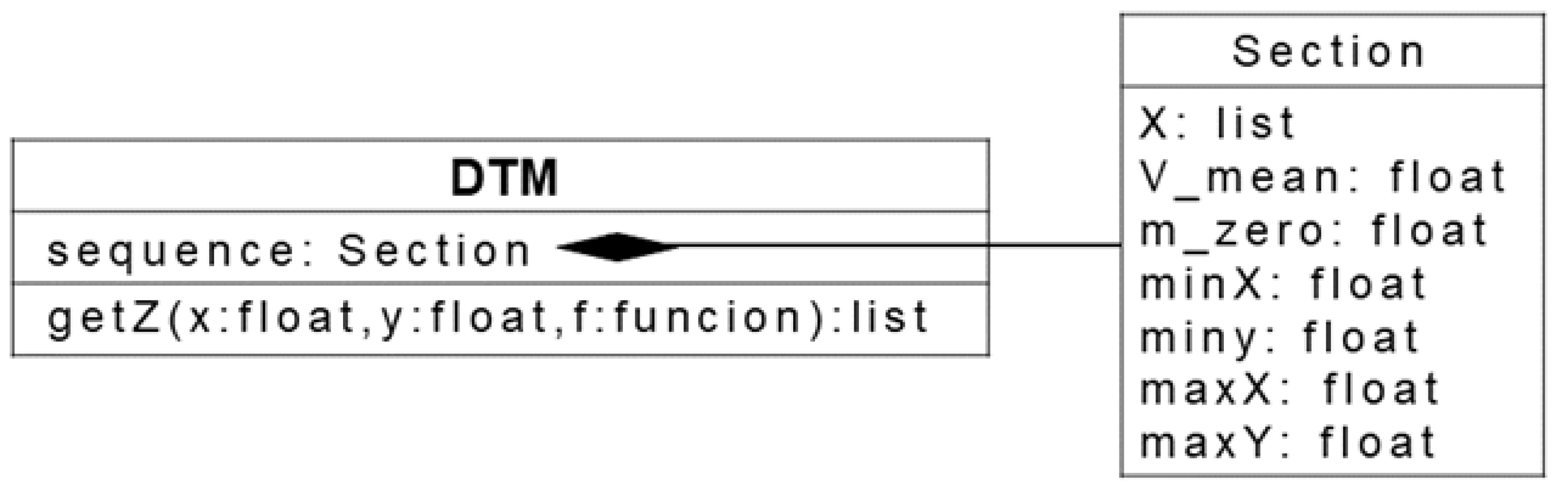
- and storing models in the form a characteristics file (a new concept in the literature on the subject), which contains all the necessary information about the model and requires a small amount of disk space (solution to p5). By using this approach, it is possible to determine the real height of any point on the object.
2. Materials and Methods
2.1. Data Reduction with the OptD Method
- uniform grid sampling, which involves dividing the point cloud space into a 3D grid of voxels and selecting one representative point from each voxel;
- voxel grid filtering, where a voxel (3D pixel) is created, and one point (usually the centroid) is chosen to represent all points within that voxel;
- random sampling, which selects a subset of points from the point cloud, though this might not preserve structure well;
- octree-based down-sampling by designing an octree data structure to subdivide the point cloud into hierarchical levels, selecting points based on resolution.
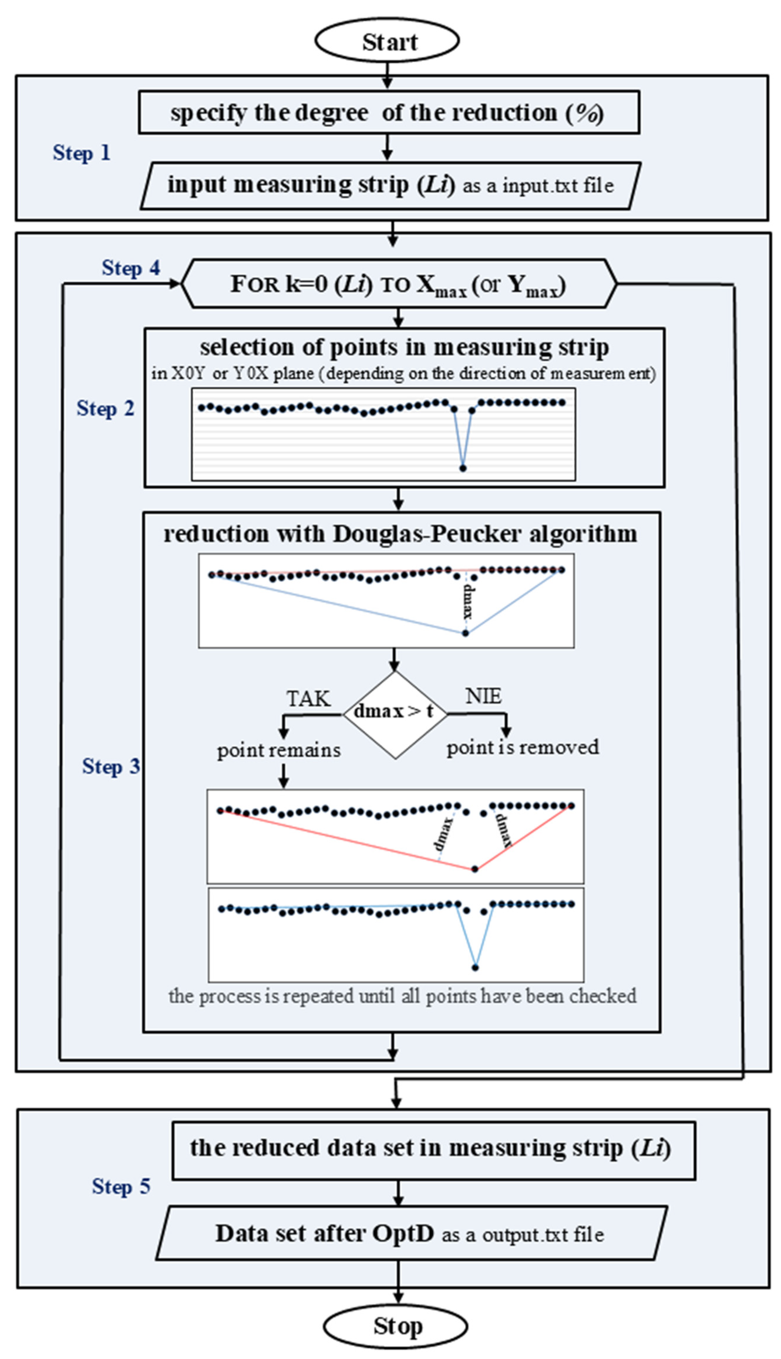
- Initial data input. The percentage of points that should remain in the dataset after reduction is determined. Then, the acquired fragment of the dataset is loaded. This fragment contains points that, in the X0Y or Y0X plane (depending on the measurement direction), define the end of the dataset;
- 2.
- Projection and preprocessing. To maintain the spatial characteristics of the points, the data are projected onto the X0Z or Y0Z plane instead of the X0Y plane;
- 3.
- Generalization using the Douglas–Peucker algorithm [34]. The algorithm simplifies a line by reducing the number of points while preserving its overall shape. It connects the start and end points of a segment and calculates the perpendicular distance of all intermediate points. Points with a distance (d) below a predefined tolerance (t) are removed, as they do not significantly impact the line’s geometry. This process is recursively repeated until no more points can be removed without exceeding the tolerance;
- 4.
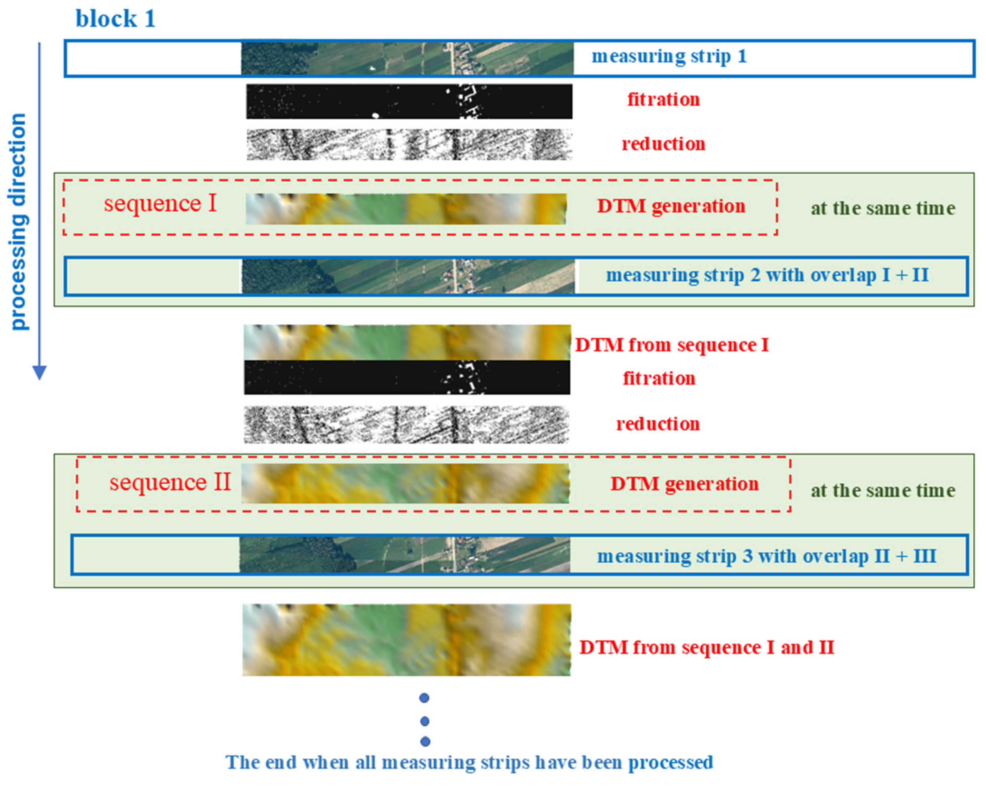
- Iterative processing. A reduced dataset representing the loaded measuring strip is obtained. While the reduction is in progress, the next measuring strip is already being acquired. Once it reaches the required width (determined by the user and measurement type), it enters the OptD algorithm for reduction;
- 5.
- Final data output. The process repeats until the last acquired measuring strip undergoes reduction, ensuring continuous and efficient data reduction while maintaining essential structural details.
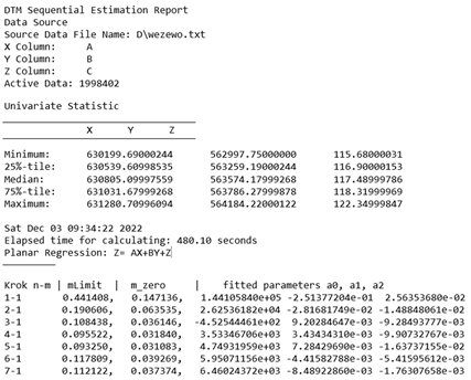
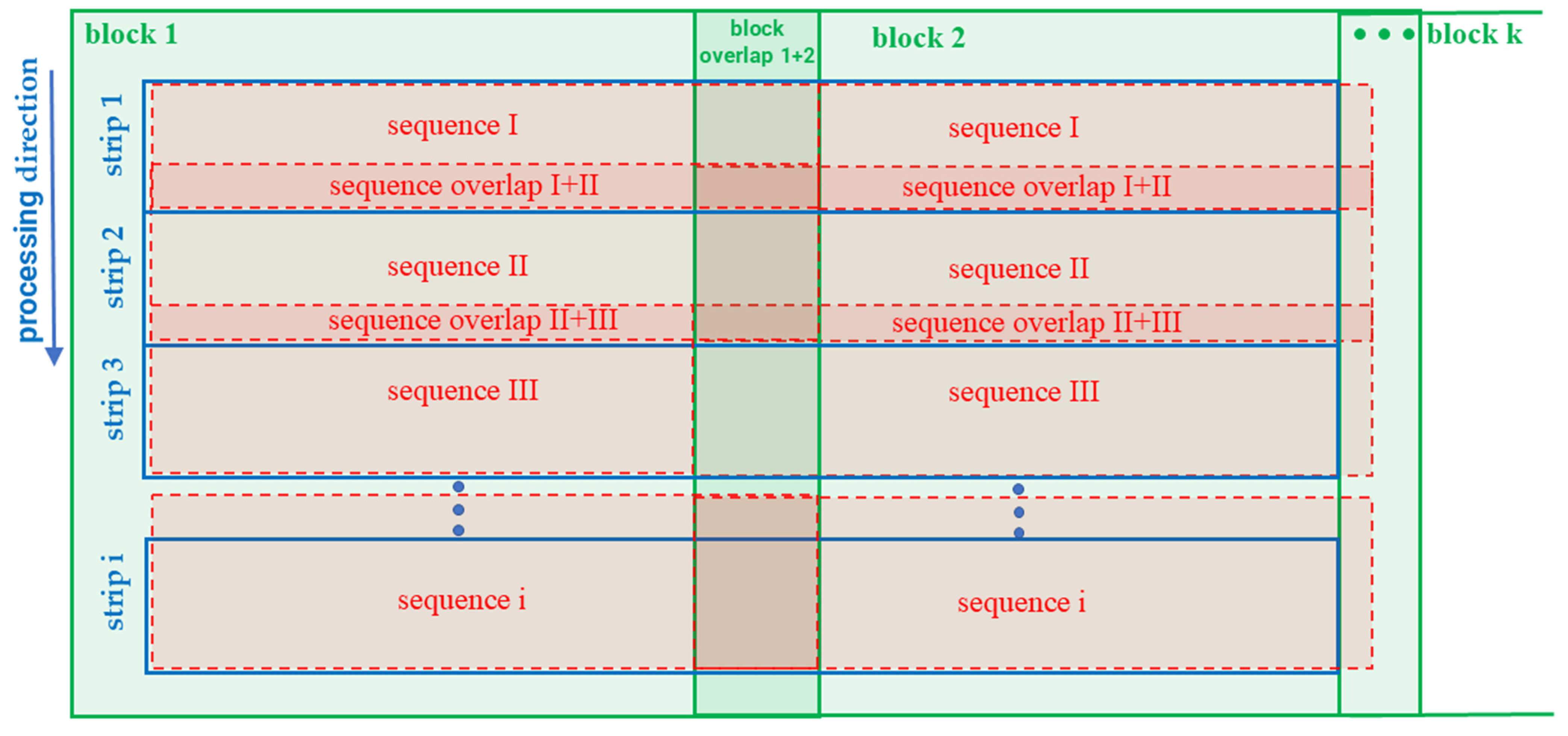
2.2. Sequential Estimation in the Context of DTM Generation
- —the vector of corrections to the intercepts of sequence II;
- —the vector of parameters obtained from sequence I included in the calculations of sequence II;
- —a known matrix of coefficients determined for the parameters of sequence I;
- —the vector of the new parameters determined in sequence II;
- —a known matrix of coefficients determined for the new parameters ;
- —the vector of intercepts of sequence II;
- —the vector of parameters (pseudo-observations) obtained from sequence I;
- —the vector of pseudo-observation corrections .
3. Results and Analysis
- One hundred points were selected from the original ALS dataset and datasets after applying the OptD method;
- The measuring strips in which individual points are located were determined;
- The parameters were found (from the characteristics file) for the sequences in which these points were located;
- The height of each point was calculated and compared with the height in the original ALS point cloud;
- The height difference was calculated.
4. Conclusions
- the use of a polynomial with higher degrees to create a DTM in more complex terrain configurations;
- the use of a sequential combination of different degrees of polynomials to approximate the measured object.
- Reduced storage space.Saving the DTM in a characteristics file (a text file) requires less computer memory compared to binary files, making data management easier;
- Analytical flexibility.Characteristics files contain essential model information, allowing for height determination at any point after processing;
- Increased processing efficiency.The OptD method reduces datasets, improving the efficiency and effectiveness of observations processed via sequential estimation;
- Variable DTM accuracy.The model shows varying accuracy across different fragments, allowing for tailored precision based on terrain conditions, unlike traditional methods;
- Potential for further development.The methodology supports future research, including the use of higher-degree polynomials for complex terrain modeling;
- Application in data acquisition systems.The method is suitable for implementation in systems that facilitate mass data collection, enhancing its practical utility in various fields.
Author Contributions
Funding
Institutional Review Board Statement
Informed Consent Statement
Data Availability Statement
Conflicts of Interest
Appendix A
References
- Hodge, V.J.; Austin, J. A survey of outlier detection methodologies. Artif. Intell. Rev. 2004, 22, 85–126. [Google Scholar] [CrossRef]
- Zhang, W.; Qi, J.; Wan, P.; Wang, H.; Xie, D.; Wang, X.; Yan, G. An easy-to-use airborne LiDAR data filtering method based on cloth simulation. Remote Sens. 2016, 8, 501. [Google Scholar] [CrossRef]
- Glira, P.; PfeifeR, N.; Briese, C.; ReSSl, C. A correspondence framework for ALS strip adjustments based on variants of the ICP algorithm. Photogramm. Fernerkund. Geoinf. 2015, 2015, 275–289. [Google Scholar] [CrossRef]
- Khosravipour, A.; Isenburg, M.; Skidmore, A.K.; Wang, T. Creating better digital surface models from LiDAR points. In Proceedings of the ACRS 2015—36th Asian Conference on Remote Sensing: Fostering Resilient Growth in Asia, Proceedings, Quezon City, Philippines, 24–28 October 2015. [Google Scholar]
- Blaszczak-Bak, W.; Pajak, K.; Sobieraj, A. Influence of datasets decreased by applying reduction and generation methods on digital Terrain models. Acta Geodyn. Geomater. 2016, 13, 361–366. [Google Scholar] [CrossRef]
- Andrew, J.T.A.; Tanay, T.; Morton, E.J.; Griffin, L.D. Transfer Representation-Learning for Anomaly Detection. In Proceedings of the 33rd International Conference on Machine Learning Research, New York, NY, USA, 19–24 June 2016; Volume 48. [Google Scholar]
- Breunig, M.M.; Kriegel, H.P.; Ng, R.T.; Sander, J. LOF: Identifying Density-Based Local Outliers. In Proceedings of the SIGMOD 2000—Proceedings of the 2000 ACM SIGMOD International Conference on Management of Data, Dallas, TX, USA, 16–18 May 2000. [Google Scholar] [CrossRef]
- Pirotti, F.; Ravanelli, R.; Fissore, F.; Masiero, A. Implementation and assessment of two density-based outlier detection methods over large spatial point clouds. Open Geospat. Data Softw. Stand. 2018, 3, 14. [Google Scholar] [CrossRef]
- Liu, Y.; Bates, P.D.; Neal, J.C. Bare-earth DEM generation from ArcticDEM and its use in flood simulation. Nat. Hazards Earth Syst. Sci. 2023, 23, 375–391. [Google Scholar] [CrossRef]
- Blaszczak-Bak, W.; Janowski, A.; Kamiñski, W.; Rapiñski, J. Optimization algorithm and filtration using the adaptive TIN model at the stage of initial processing of the ALS point cloud. Can. J. Remote Sens. 2012, 37, 583–589. [Google Scholar] [CrossRef]
- Graham, A.; Coops, N.C.; Wilcox, M.; Plowright, A. Evaluation of ground surface models derived from unmanned aerial systems with digital aerial photogrammetry in a disturbed conifer forest. Remote Sens. 2019, 11, 84. [Google Scholar] [CrossRef]
- Zhou, S.; Zhang, Y.; Yang, J. 3D Mathematical Modeling and Visualization Application Based on Virtual Reality Technology. Comput. Aided Des. Appl. 2023, 20, 1–13. [Google Scholar] [CrossRef]
- Abdeldayem, Z. Automatic Weighted Splines Filter (AWSF): A New Algorithm for Extracting Terrain Measurements from Raw LiDAR Point Clouds. IEEE J. Sel. Top. Appl. Earth Obs. Remote Sens. 2020, 13, 60–71. [Google Scholar] [CrossRef]
- Stereńczak, K.; Ciesielski, M.; Bałazy, R.; Zawiła-Niedźwiecki, T. Comparison of various algorithms for DTM interpolation from LIDAR data in dense mountain forests. Eur. J. Remote Sens. 2016, 49, 599–621. [Google Scholar] [CrossRef]
- Thomas, K. A New Simplified DSM-to-DTM Algorithm-dsm-to-dtm-step. Preprints 2018, 1, 1–10. [Google Scholar]
- Hodgson, M.E.; Bresnahan, P. Accuracy of Airborne Lidar-Derived Elevation. Photogramm. Eng. Remote Sens. 2013, 70, 331–339. [Google Scholar] [CrossRef]
- Wechsler, S.P. Uncertainties associated with digital elevation models for hydrologic applications: A review. Hydrol. Earth Syst. Sci. 2007, 11, 1481–1500. [Google Scholar] [CrossRef]
- Rehman, M.H.U.; Liew, C.S.; Abbas, A.; Jayaraman, P.P.; Wah, T.Y.; Khan, S.U. Big Data Reduction Methods: A Survey. Data Sci. Eng. 2016, 1, 265–284. [Google Scholar] [CrossRef]
- Mujta, W.; Wlodarczyk-Sielicka, M.; Stateczny, A. Testing the Effect of Bathymetric Data Reduction on the Shape of the Digital Bottom Model. Sensors 2023, 23, 5445. [Google Scholar] [CrossRef]
- Jain, K.; Murty, P.; Flynn, J. Data clustering: A review. ACM Comput. Surv. 1999, 31, 264–323. [Google Scholar] [CrossRef]
- Rusu, R.B.; Cousins, S. 3D is here: Point Cloud Library (PCL). In Proceedings of the IEEE International Conference on Robotics and Automation, Shanghai, China, 9–13 May 2011. [Google Scholar] [CrossRef]
- El-Sayed, E.; Abdel-Kader, R.F.; Nashaat, H.; Marei, M. Plane detection in 3D point cloud using octree-balanced density down-sampling and iterative adaptive plane extraction. IET Image Process. 2018, 12, 1595–1605. [Google Scholar] [CrossRef]
- Błaszczak-Bąk, W. New optimum dataset method in LiDAR processing. Acta Geodyn. Geomater. 2016, 13, 381–388. [Google Scholar] [CrossRef]
- Liu, Y.; Zhang, Y.; Chao, H. Incremental Fuzzy Clustering Based on Feature Reduction. J. Electr. Comput. Eng. 2022, 2022, 8566253. [Google Scholar] [CrossRef]
- Du, X.; Zhuo, Y. A point cloud data reduction method based on curvature. In Proceedings of the 2009 IEEE 10th International Conference on Computer-Aided Industrial Design and Conceptual Design: E-Business, Creative Design, Manufacturing—CAID and CD’2009, Wenzhou, China, 26–29 November 2009; pp. 914–918. [Google Scholar] [CrossRef]
- Błaszczak-Bąk, W.; Sobieraj-Żłobińska, A.; Wieczorek, B. The Optimum Dataset method–examples of the application. E3S Web Conf. 2018, 26, 00005. [Google Scholar]
- Błaszczak-Bąk, W.; Sobieraj-Żłobińska, A.; Kowalik, M. The OptD-multi method in LiDAR processing. Meas. Sci. Technol. 2017, 28, 7500–7509. [Google Scholar]
- Rashdi, R.; Martínez-Sánchez, J.; Arias, P.; Qiu, Z. Scanning Technologies to Building Information Modelling: A Review. Infrastructures 2022, 7, 49. [Google Scholar] [CrossRef]
- Siewczyńska, M.; Zioło, T. Analysis of the Applicability of Photogrammetry in Building Façade. Civ. Environ. Eng. Rep. 2022, 32, 182–206. [Google Scholar] [CrossRef]
- Sánchez-Aparicio, L.J.; Del Pozo, S.; Ramos, L.F.; Arce, A.; Fernandes, F.M. Heritage site preservation with combined radiometric and geometric analysis of TLS data. Autom. Constr. 2018, 85, 24–39. [Google Scholar] [CrossRef]
- Pajak, K.; Blaszczak-Bak, W. Baltic sea level changes from satellite altimetry data based on the OptD method. Acta Geodyn. Geomater. 2019, 16, 235–244. [Google Scholar] [CrossRef]
- Suchocki, C.; Błaszczak-Bąk, W.; Janicka, J.; Dumalski, A. Detection of defects in building walls using modified OptD method for down-sampling of point clouds. Build. Res. Inf. 2020, 49, 197–215. [Google Scholar] [CrossRef]
- Błaszczak-Bąk, W.; Janicka, J.; Suchocki, C.; Masiero, A.; Sobieraj-żłobińska, A. Down-Sampling of large lidar dataset in the context of off-road objects extraction. Geosciences 2020, 10, 219. [Google Scholar] [CrossRef]
- Douglas, D.H.; Peucker, T.K. Algorithms for the reduction of the number of points required to represent a digitized line or its caricature. Can. Cartogr. 1973, 10, 112–122. [Google Scholar] [CrossRef]
- Gao, B.; Hu, G.; Li, W.; Zhao, Y.; Zhong, Y. Maximum Likelihood-Based Measurement Noise Covariance Estimation Using Sequential Quadratic Programming for Cubature Kalman Filter Applied in INS/BDS Integration. Math. Probl. Eng. 2021, 2021, 9383678. [Google Scholar] [CrossRef]
- Tan, L.; Wang, Y.; Hu, C.; Zhang, X.; Li, L.; Su, H. Sequential Fusion Filter for State Estimation of Nonlinear Multi-Sensor Systems with Cross-Correlated Noise and Packet Dropout Compensation. Sensors 2023, 23, 4687. [Google Scholar] [CrossRef] [PubMed]
- Kim, T.; Park, T.H. Extended kalman filter (Ekf) design for vehicle position tracking using reliability function of radar and lidar. Sensors 2020, 20, 4126. [Google Scholar] [CrossRef]
- Habib, A.; Bang, K.I.; Kersting, A.P.; Chow, J. Alternative methodologies for LiDAR system calibration. Remote Sens. 2010, 2, 874. [Google Scholar] [CrossRef]
- Rentsch, M.; Krzystek, P. Precise quality control of LiDAR strips. In Proceedings of the American Society for Photogrammetry and Remote Sensing Annual Conference 2009, ASPRS 2009, Baltimore, MD, USA, 9–13 March 2009. [Google Scholar]
- Alsadik, B.; Remondino, F. Flight planning for LiDAR-based UAS mapping applications. ISPRS Int. J. Geo inf. 2020, 9, 378. [Google Scholar] [CrossRef]
- Mastor, T.A.; Kamarulzaman, N.; Abidin, M.M.; Samad, A.M.; Hashim, K.A.; Maarof, I.; Zainuddin, K. The Unmanned Aerial Imagery Capturing System (UAiCs) flight planning calculation parameters for small scale format imagery. In Proceedings of the Proceedings—2014 5th IEEE Control and System Graduate Research Colloquium, ICSGRC 2014, Shah Alam, Malaysia, 11–12 August 2014. [Google Scholar] [CrossRef]
- Axelsson, P. DEM Generation from Laser Scanner Data Using adaptive TIN Models. Int. Arch. Photogramm. Remote Sens. 2000, 23, 110–117. [Google Scholar]
- Arun, P.V. A comparative analysis of different DEM interpolation methods. Egypt. J. Remote Sens. Space Sci. 2013, 16, 133–139. [Google Scholar] [CrossRef]
- Candia-Rivera, D.; Valenza, G. Cluster permutation analysis for EEG series based on non-parametric Wilcoxon–Mann–Whitney statistical tests. SoftwareX 2022, 19, 101170. [Google Scholar] [CrossRef]

| Reduction Method | Principle | Data Retention | Computational Efficiency | Impact on Accuracy |
|---|---|---|---|---|
| Uniform grid sampling [20] | Divides the space into a 3D grid and selects one representative point per voxel. | Moderate (depends on grid resolution) | High (fast processing) | Moderate (loss of fine details in high-density areas) |
| Voxel grid filtering [21] | Averages points within a voxel to reduce redundancy. | High (preserves general structure) | High (efficient for large datasets) | Moderate (smooths surfaces but may remove small features) |
| Random sampling [18] | Randomly selects a subset of points. | Low (risk of missing key features) | Very high (minimal computation required) | High (loss of critical terrain details) |
| Octree-based downsampling [22] | Hierarchically subdivides the point cloud and selects representative points at each level. | High (adaptive retention) | Moderate (depends on depth of octree) | Low (preserves key structures well) |
| Feature-based reduction [18] | Prioritizes points with high curvature or unique geometric properties. | Very high (retains essential features) | Low (computationally intensive) | Very Low (preserves critical details accurately) |
| OptD method (proposed) [23] | Selects optimal points based on optimization criteria (e.g., percentage retained, tolerance). | Customizable (user-defined) | High (adaptive and efficient) | Low (maintains accuracy while reducing redundancy) |
| Variant | v.1 | v.2 | ||||
|---|---|---|---|---|---|---|
| Percentage of Points in Dataset | [m] | |||||
| Min | Max | Mean | Min | Max | Mean | |
| 100% | 0.000 | 1.115 | 0.051 | 0.000 | 1.375 | 0.073 |
| 50% | 0.000 | 0.538 | 0.051 | 0.000 | 1.132 | 0.073 |
| 30% | 0.000 | 0.541 | 0.053 | 0.000 | 0.816 | 0.070 |
| 10% | 0.001 | 0.602 | 0.062 | 0.000 | 1.125 | 0.083 |
| 2% | 0.001 | 0.590 | 0.086 | 0.001 | 1.137 | 0.123 |
| Variant | v.1 | v.2 | ||
|---|---|---|---|---|
| Reference DTM | RMSE [m] | Speed [s] | RMSE [m] | Speed [s] |
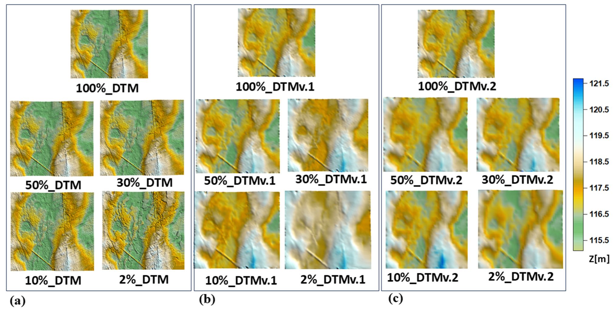
| 100%_DTM | 0.104 | 480 | 0.098 | 398 |
| 50%_DTM | 0.051 | 160 | 0.074 | 154 |
| 30%_DTM | 0.041 | 135 | 0.043 | 126 |
| 10%_DTM | 0.052 | 71 | 0.103 | 63 |
| 2%_DTM | 0.121 | 36 | 0.099 | 26 |
| Variant | v.1 | v.2 | ||
|---|---|---|---|---|
| Percentage of Points in Dataset | [m] | |||
| Min | Max | Min | Max | |
| 100% | 0.010 | 0.526 | 0.011 | 0.475 |
| 50% | 0.012 | 0.639 | 0.010 | 0.532 |
| 30% | 0.011 | 0.621 | 0.021 | 0.613 |
| 10% | 0.020 | 0.711 | 0.120 | 0.825 |
| 2% | 0.092 | 0.752 | 0.111 | 0.537 |
Disclaimer/Publisher’s Note: The statements, opinions and data contained in all publications are solely those of the individual author(s) and contributor(s) and not of MDPI and/or the editor(s). MDPI and/or the editor(s) disclaim responsibility for any injury to people or property resulting from any ideas, methods, instructions or products referred to in the content. |
© 2025 by the authors. Licensee MDPI, Basel, Switzerland. This article is an open access article distributed under the terms and conditions of the Creative Commons Attribution (CC BY) license (https://creativecommons.org/licenses/by/4.0/).
Share and Cite
Błaszczak-Bąk, W.; Kamiński, W.; Bednarczyk, M.; Suchocki, C.; Masiero, A. Real-Time DTM Generation with Sequential Estimation and OptD Method. Appl. Sci. 2025, 15, 4068. https://doi.org/10.3390/app15074068
Błaszczak-Bąk W, Kamiński W, Bednarczyk M, Suchocki C, Masiero A. Real-Time DTM Generation with Sequential Estimation and OptD Method. Applied Sciences. 2025; 15(7):4068. https://doi.org/10.3390/app15074068
Chicago/Turabian StyleBłaszczak-Bąk, Wioleta, Waldemar Kamiński, Michał Bednarczyk, Czesław Suchocki, and Andrea Masiero. 2025. "Real-Time DTM Generation with Sequential Estimation and OptD Method" Applied Sciences 15, no. 7: 4068. https://doi.org/10.3390/app15074068
APA StyleBłaszczak-Bąk, W., Kamiński, W., Bednarczyk, M., Suchocki, C., & Masiero, A. (2025). Real-Time DTM Generation with Sequential Estimation and OptD Method. Applied Sciences, 15(7), 4068. https://doi.org/10.3390/app15074068