The Automatic Algorithm of Optimizing the Position of Structured Light Sensors

Abstract

Optical 3D detection technology has a wide range of applications in industrial detection, agricultural production, and so on. Its advantages are non-contact, efficiency, and high precision. However, the specular reflection problem affects model coverage and measurement accuracy. An optimization algorithm for calculating the number and pose of sensors has been proposed to address this issue. First, the specular reflection problem is viewed as a multi-sensor position search problem. Then, an optimization algorithm is used to find the optimal number and bit positions of sensors to avoid specular reflection. The experiment shows that the optimization results of this algorithm can cover the area to be measured with the least number of sensor combinations while avoiding the influence of specular reflection.

1. Introduction

With the rapid development of modern industrial fields such as ships, automobiles, aerospace, and molds, not only the requirements for product design and manufacturing are increasingly increasing, but also the testing requirements for product processing are more stringent. The traditional 3D detection equipment, such as 3D coordinate machines, has limited measurement efficiency and easy wear on the surface of the workpiece. In the past few decades, remarkable progress has been made in non-contact 3D morphology reconstruction techniques. Among them, structural optical measurement technology has been widely used in the field of high-precision measurement, such as product processing, because of its non-contact nature, large range, high efficiency, and high precision. The development of this technology not only improves measurement efficiency but also reduces interference to the surface of the workpiece, meeting the growing demand of modern industry for product quality and precision. However, in this process, the specular reflection problem [1] seriously reduces the accuracy of 3D measurement. Therefore, dealing with the specular reflection problem is a crucial consideration in structured light 3D measurement applications. To cope with this problem, a series of effective methods are required.

There are six main categories of technologies to address specular reflections: polarization technology, structured light intensity adjustment, fully automatic exposure, reflective component separation technology, multi-angle shooting technology, and sensor setting optimization algorithms.

To address the problem of highlights in 3D measurements, some researchers [2,3,4,5,6] have used the technique of polarization to deal with highlights during the measurement process. Zhu et al. [2] proposed a polarization-based highlight removal method in order to achieve highlight removal from high-reflectivity surfaces. In the polarization-based method, images are captured at different polarization angles, and multiple polarized images are synthesized to reduce the highlight brightness. A normalized weighting algorithm is also used to recover the highlights that cannot be recovered by the polarization image synthesis. Zhu et al. [3] proposed a polarization-based method for three-dimensional measurement of the light intensity response function of a camera. The light intensity response function of the camera under the polarization system was established. The method avoids the complex model of the polarization bidirectional reflection distribution function and directly quantifies the required angle between the transmission axes of two polarization filters. It is then combined with an image fusion algorithm to generate an optimal streak map. Moreover, the high signal-to-noise ratio and contrast of the image are maintained after adding the polarization filter. Kong et al. [4] designed a measurement system to acquire images with different polarization angles, and the highlighted areas in the images are used as training samples for the BP neural network. The initial weights of the neural network are Gaussian distributions. The stereo matching accuracy can be effectively improved so as to recover the information from specular vision measurements in the highlighted region. Liang et al. [5] proposed a polarized structured light method to solve the problem of the reconstruction of high-reflectivity surfaces. The built-in structured light system involves a four-channel polarization camera and a digital light processing (DLP) projector equipped with a polarizer lens. The built-in system is capable of simultaneously acquiring four sets of streak images, each with a different luminance difference. Then, a binary time-multiplexed structured light method is used to acquire four different point clouds. The proposed method has been shown to achieve excellent reconstruction results on highly reflective surfaces. Huang et al. [6] devise a polarization-structured light 3D sensor for solving these problems, in which high-contrast-grating (HCG) vertical-cavity surface-emitting lasers (VCSELs) are used to exploit the polarization property.

A few researchers [7,8,9,10] dealt with the high-light problem by adjusting the light intensity of the projection pattern. Lin et al. [7] proposed a method to automatically determine the optimal number of light intensities and the corresponding light intensity values for streak map projection based on the surface reflectance of the object under test. The original streak images captured under different light intensities are synthesized pixel by pixel into a composite streak image, which can be further used for phase recovery and conversion to 3D coordinates. Cao et al. [8] used a transparent screen as an optical mask for the camera so as to indirectly adjust the intensity of the projected pattern. By placing a transparent screen in front of the camera and adjusting the luminance of the corresponding screen pixels, the brightness of each pixel of the camera can be precisely controlled. precisely control the brightness of each pixel of the camera. Fu et al. [9] proposed a set of hardware devices and region-adaptive structured light algorithms. Based on the accurate optical modeling of the measurement scene, the principles for generating the adaptive optimal projection brightness are derived in detail, and the process is accelerated by exploiting the speed of the neural network. Meanwhile, they creatively use the chain code combined with the M-estimator sample consensus method to find the homography from the saturated region of the cam-era plane to the corresponding region of the projector plane for generating fringe images with adaptive brightness. Furthermore, they chose the more robust line-shifting code and binarization method for subpixel 3D reconstruction. Zhou et al. [10] proposed a method. The multi-intensity projection method was adopted by reducing the input projection intensity step-by-step and reconstructing the remaining pixels around the specular angle. Finally, the reconstruction result can be obtained by stitching point clouds at each projection intensity. Experiments verified that the proposed method could improve the integrity of reconstructed point clouds and measurement efficiency.

Rao et al. [11] proposed a stripe projection contouring method based on fully automated multiple exposures, which requires human intervention and greatly simplifies the whole reconstruction process. It is mathematically proven that once the modulation of a pixel is greater than a threshold value, the phase quality of that pixel can be considered satisfactory. This threshold can be used to guide the calculation of the required exposure time. The software then automatically adjusts the exposure time of the camera and captures the desired streak images. Using these captured images, a final reconstruction with a high dynamic range can be easily obtained. Wu et al. [12] proposed an exposure fusion (EF)-based structured light method to accurately reconstruct a three-dimensional model of the object with a special reflective surface. A robust binary gray code is adopted as our structured light pattern. They fuse a group of images with different exposure times into a single image with a high dynamic range. With the help of the EF technique, captured images that have many overexposed and underexposed regions can be well exposed. The EF method, which has a simple operational procedure, is adopted in their work. Based on the EF method, precise 3D reconstruction of a reflective surface can be realized. Song et al. [13] proposed a novel structured light approach for the 3D reconstruction of specular surfaces. The binary shifting strip is adopted as a structured light pattern instead of a conventional sinusoidal pattern. Based on the framework of conventional high-dynamic range imaging techniques, an efficient means is first introduced to estimate the camera response function. Then, the dynamic range of the generated radiance map is compressed in the gradient domain by introducing an attenuation function. Subject to the change in lighting conditions caused by projecting different structured light patterns, the structure light image with the middle exposure level is selected as the reference image and used for the slight adjustment of the primary fused image. Finally, the regenerated structured light images with well-exposing conditions are used for 3D reconstruction of the specular surface. To evaluate the performance of the method, some stainless steel stamping parts with strong reflectivity were used for the experiments. The results showed that different specular targets with various shapes can be precisely reconstructed by the proposed method.

Sun et al. [14] designed a new algorithm based on reflective component separation (RCS) and priority region filling theory. The specular pixels in the image are first found by comparing the pixel parameters. Then, the reflection components are separated and processed. However, for objects such as ceramics and metals with strong specular highlights, the RCS theory will change the color information of the highlight pixels due to the larger specular reflection component. In this case, the preferred region filling theory is used to recover the color information. Schematic diagram of the principle of multi-angle measurement: the basic idea is to collect images of the same object from different angles so that the highlight areas of different images do not overlap, thus recovering data from the same scene. There are many subsequent data processing methods, which can be used with binocular vision [15,16,17,18], monocular structured light, or directly using the parallax method to recover depth information.

Qian et al. [19] came up with a computational method to compute the optimal sensor setup, taking into account sensor/part interactions, in order to reduce the dynamic range of the signal and increase the model coverage of structured light or similar optical detection systems. First, the signal dynamic range problem is transformed into a distance problem in spherical mapping. Then, a new algorithm on the spherical map is proposed to search for a near-optimal sensor orientation. Based on this near-optimal orientation, to obtain the optimal solution, make the lowest possible dynamic range. However, Qian [19] only optimizes for a group of sensor systems and not for multi-sensor systems.

The polarization-based measurement method can effectively reduce the specular reflection problem, but the hardware requirements are relatively high. Structural light intensity adjustment technology, from the light source to reduce the probability of specular reflection, has high hardware requirements but also requires calculating the correlation coefficient of the intensity of the light source. The fully automated exposure technology solves the problem of specular reflection from the angle of the shooting, but it may lead to part of the surface brightness being too dark, as well as the need for large-scale splicing. The reflection component separation technology solves the specular reflection problem by separating the reflection information, but when the specular reflection intensity is high, there will be a loss of information. Multi-angle shooting technology shoots from multiple angles, but it cannot automatically optimize the number of devices and positional information. Sensor setup optimization technology optimizes specular reflection for a single device on a flat surface, but it does not optimize multiple devices on the whole surface of the object to measure specular reflection. The sensor setup optimization technique optimizes the specular reflection of a single device for a flat surface but not for the whole surface of the object.

In order to solve the above-mentioned specular reflection problem, an optimization method is proposed to calculate the positions that can avoid specular reflection for any object. This method solves the problem: when using multi-angle methods in the presence of specular reflection areas, optimize the corresponding optimal number of sensors and specific positions.

The second part introduces the optimization method for the number and position of multiple sensors. The third part introduces simulation experiments and validation experiments. The fourth part is a summary.

2. Optimization Method for the Number and Position of Multiple Sensors

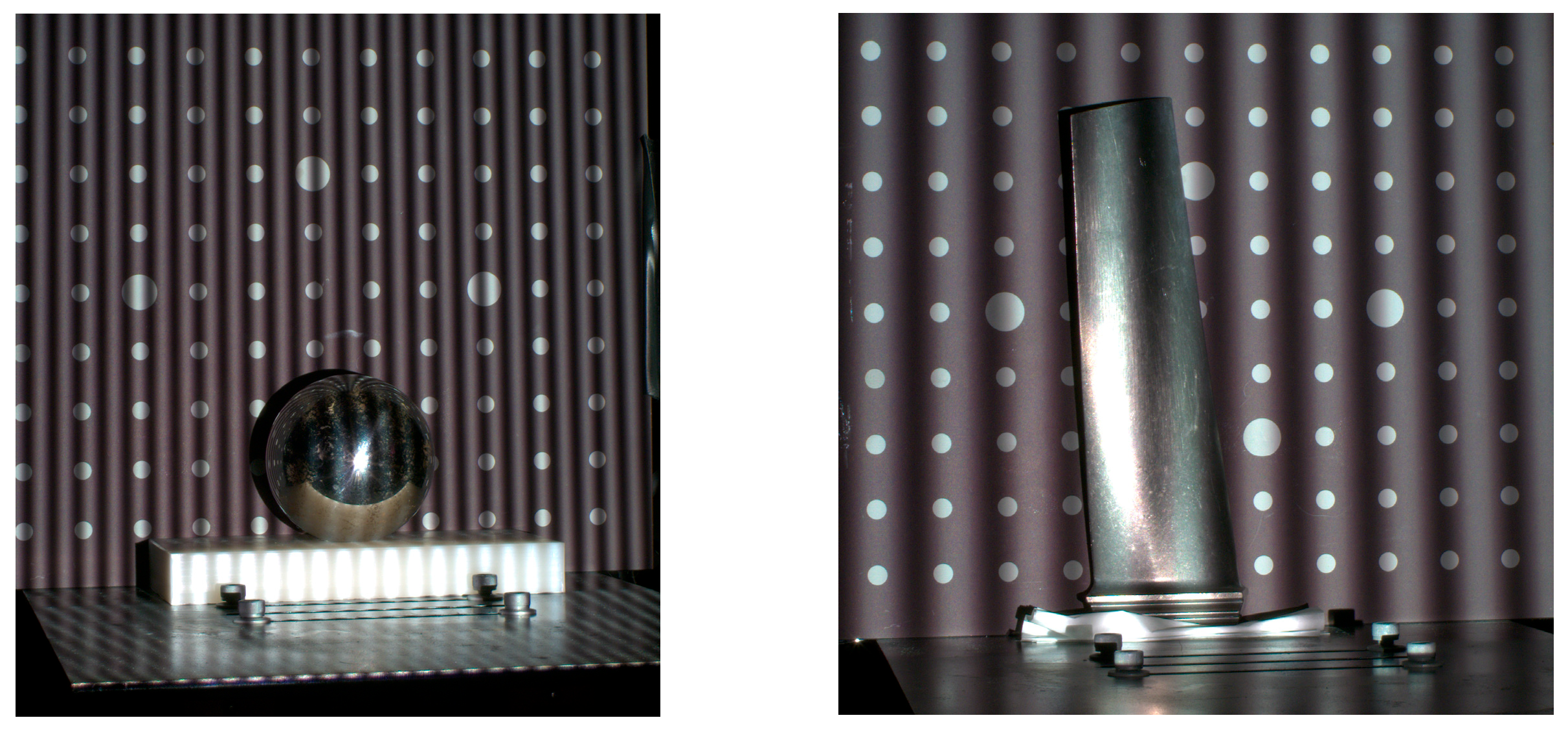
Objects with high reflection coefficients, such as metals, are also objects of three-dimensional measurement. However, in actual measurements, there are often several specular reflection areas, which leads to a loss of measurement information and affects the measurement. The specular reflection areas are shown in Figure 1. Multi-angle is one of the methods used to solve the problem of specular reflection. The principle of a multi-angle sensor is shown in Figure 2, taking two sets of sensors as an example. The specular reflection areas of the two sets of sensors are different, and the non-specular reflection areas of the two sets of sensors are complementary. By fusing the non-specular areas of two sets of sensors, the problem of specular reflection is solved. During this process, the coverage area and specular reflection area of the sensor need to be manually adjusted and optimized. Even for professionals, facing objects with diverse shapes can take a long time, and the optimized sensor positions and quantities may not necessarily be optimal.

However, some people’s research has focused on the method of multi-angle sensors, and no one has paid attention to this issue: when using multi-angle methods in the presence of specular reflection areas, optimize the corresponding optimal number of sensors and specific positions. Aiming at this issue, this article proposes an automatic algorithm for optimizing the position of structured light sensors.

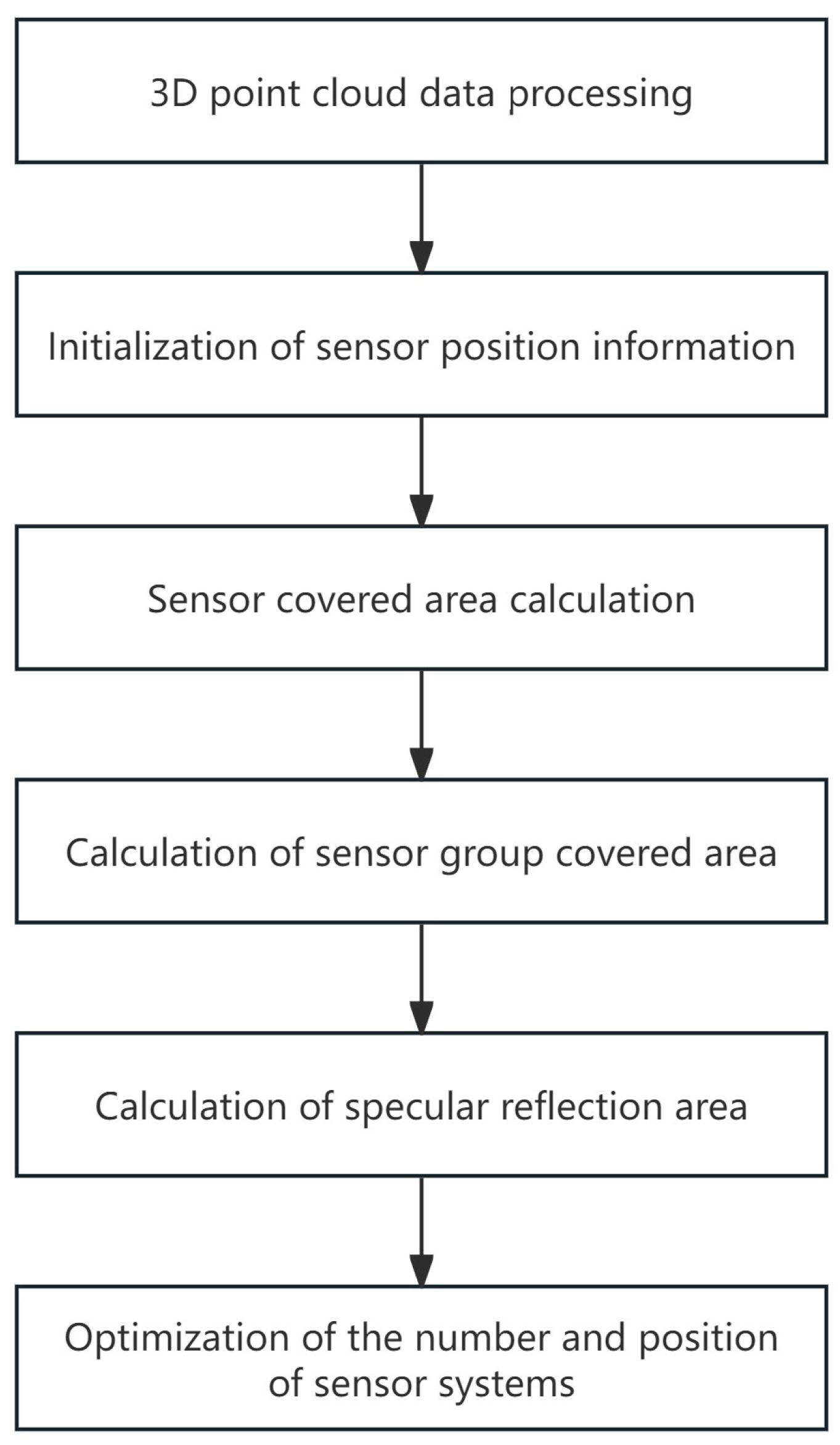
The overall idea of the system optimization algorithm is shown in Figure 3. First, the 3D point cloud data is processed, and then the sensor position information is initialized. A 3D point cloud can be obtained from the design document. Next, the sensor coverage area is analyzed based on the calculation of the coverage area of the sensor group. Furthermore, the specular reflection area of the sensor group is calculated, and finally the position and pose of the sensor are optimized.

2.1. Initialize Sensor Position Information

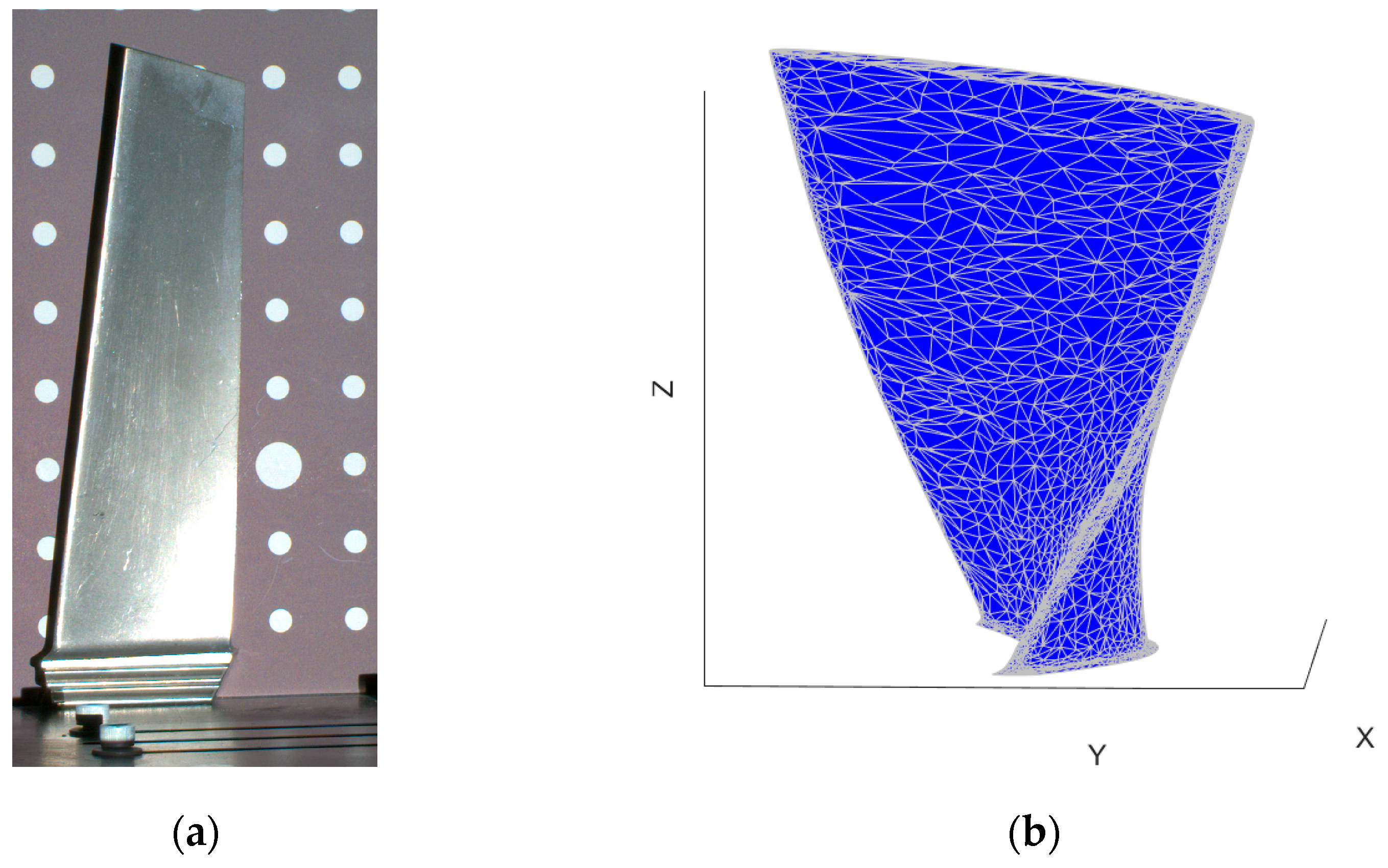
For measuring objects that already have a 3D point cloud. After obtaining the 3D object point cloud data, the sensor position information can be initialized. First, the projector was placed on a spherical surface centered on a point-cloud object. Next, based on the position of the projector, draw a circle on the outer cut plane and place the camera corresponding to the projector in that plane. Figure 4 shows the tested object (a turbine blade) and its 3D model. 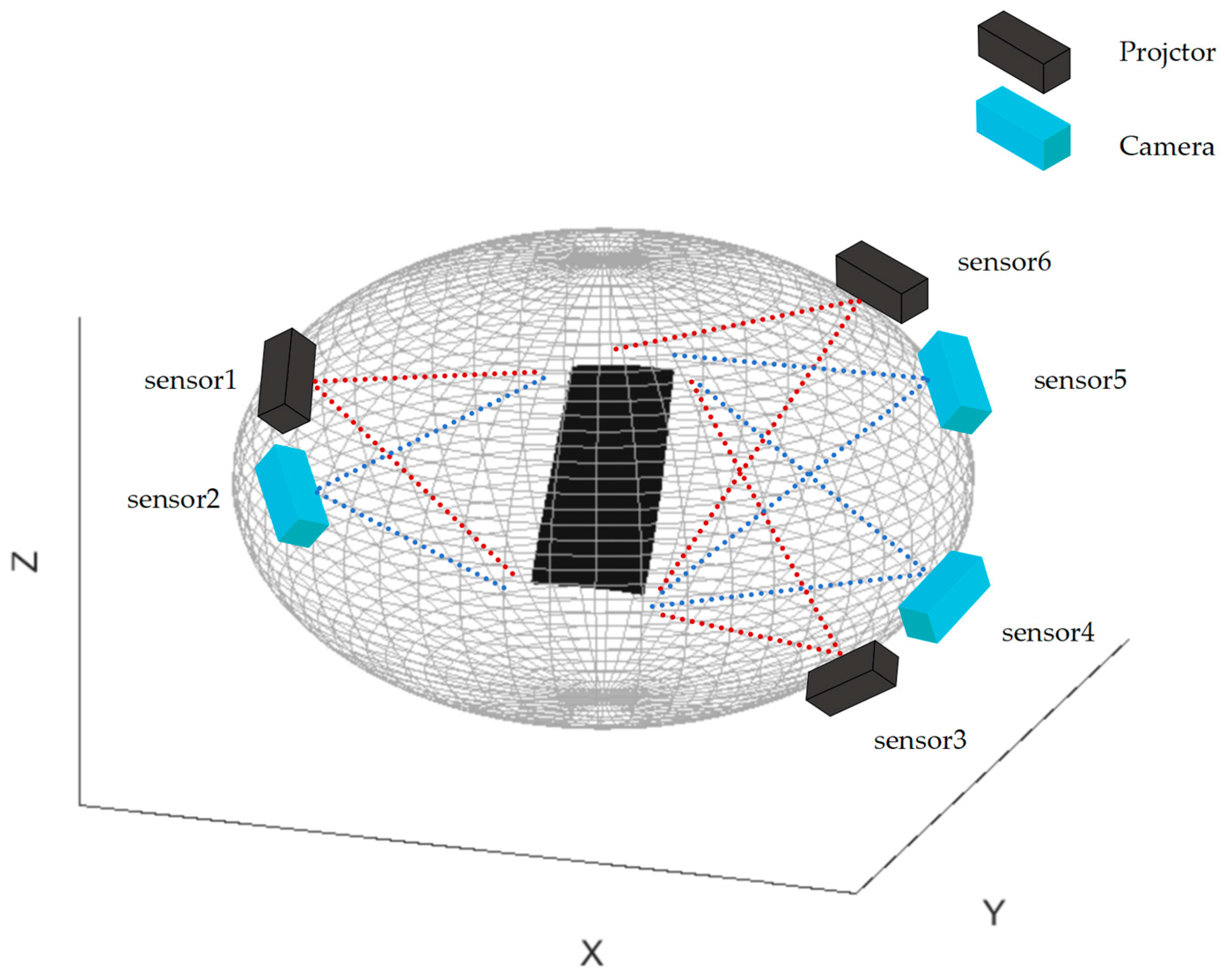Figure 5 shows the overall system schematic diagram. In Figure 5, a black box represents a projector, and a blue box represents a camera. Each box represents a sensor. The red dashed line represents the projector’s field of view, while the blue dashed line represents the camera’s field of view. The gray spherical net represents the position of the projector that can be optimized. The innermost black object is the object to be measured. Initialize several pairs of sensors based on the measured object.

2.2. Covered Area Judgment

Before the sensor correlation optimization, the first priority is to clarify the covered area of the sensor. The covered area of the projector refers to the area of the pattern projected onto the surface of the measured object, while the covered area of the camera refers to the surface area of the measured object that the camera can capture. The covered area is judged in three steps, respectively: calculating the initial covered area, calculating the covered area of the sensor, and calculating the covered area of the sensor group.

Calculating the initial covered area

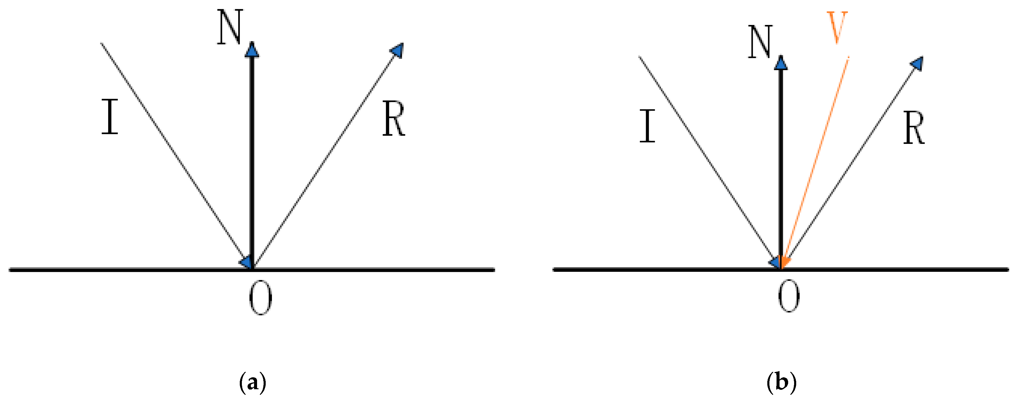
When dealing with large-scale 3D point cloud data, the computational complexity is high. Therefore, a preliminary covered area estimation is first needed to determine the possible coverage of the sensor. Figure 6a is a schematic diagram of the specular reflection of the light in the plane. Figure 6a represents the vector of the incoming light, N represents the normal vector of the surface, and R represents the specular reflection vector of the incident light I. Within the covered area of the sensor, the normal vector N of the surface and the incident vector I of the sensor are negative. The initial covered area is calculated using Equation (1). When I and N comply with Equation (1), the incident light may pass through the triangular surface where N is located. When they do not match, the incident light does not pass through the triangular surface where N is located. Next, further detection is carried out on the triangular surface that conforms to Equation (1).

Figure 6. Schematic diagram of the optical path. (a) is a schematic diagram of the specular reflection of the light in the plane. (b) is the light propagation diagram of the sensor group.

Figure 6. Schematic diagram of the optical path. (a) is a schematic diagram of the specular reflection of the light in the plane. (b) is the light propagation diagram of the sensor group.

$$I•N<0$$

(1)

Calculating the covered area of the sensor

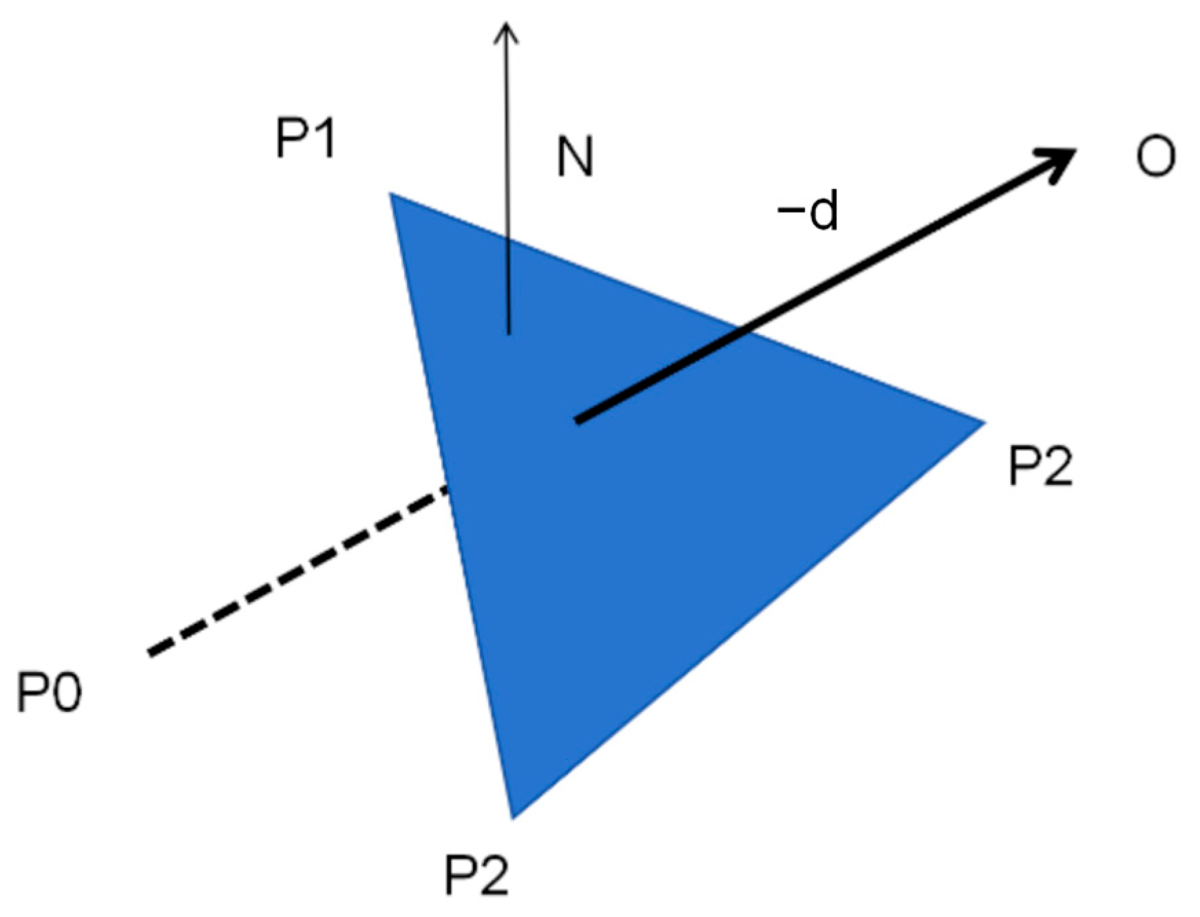
After the initial covered area calculation, there is a small portion of the surface that is not within the effective coverage area of the sensor. Therefore, an accurate sensor-covered area calculation is required to exclude the above errors. By traversing the preliminary calculated coverage area, calculate whether there are occluded surfaces between these surfaces and the sensors. If there is an obstructed surface, mark it as a non-covered area. If there is no occluded surface, it is marked as a valid coverage area. This calculation is based on the Moller-Trumbore algorithm [20]. The idea of this algorithm is shown in Figure 7. Calculation formulas such as Equations (2) and (3). In Figure 7, P₀ represents the center of gravity of the triangular face to be measured, P₁, P₂, and P₃ represent the three vertices of any other triangles that are within the initial coverage area, O represents the sensor, and -d denotes the ray direction vector pointing to O from P₀. The parameters t, b₂, and b₃ in Equation (2)), and b₁ in Equation (3) are the parameters to be solved. When all these parameters t, b₂, b₃, and b₁ are greater than 0, it means that there is an intersection of the ray with the triangular plane. Therefore, the triangular face where P₀ is not located in the effective covered area of the sensor.

Figure 7. Covered area judgment.

Figure 7. Covered area judgment.

$$O+t\times \overrightarrow{d}=(1-b_2-b{3}_3)\times P_1+b_1\times P_2+b_2\times P_3$$

(2)

$${\mathrm{b}}_1=1-b_2-b_3$$

(3)

Calculating the covered area of the sensor group

In 3D structured light measurement, each sensor group includes at least one projector and one camera. In the measurement of the sensor group, the measurement area is the intersection of the covered areas of the projector and the camera. Therefore, after the calculation of the coverage area of a single sensor is completed, calculating the coverage area of a sensor group is relatively simple and only requires determining the common coverage area of the projector and the camera.

2.3. Specular Reflection Area Identification

After calculating the coverage area of a sensor group, it is necessary to identify the specular reflection areas for each group of sensors. These areas are used as one of the parameter values optimized for the sensor system. The light propagation diagram of the sensor group is shown on the right in Figure 6b, where V is the pointing vector of the camera, I is the pointing vector of the projector, and R is the specular reflection vector of the projector’s light on the surface. Specular reflection is the specular reflection of light on the surface of a smooth object where the angle between the reflected light and the direction of observation is small. It causes the brightness of the photographed object to exceed the camera’s dynamic range, white areas to appear, and a loss of 3D measurement information. It should be noted that the specular reflection of each sensor group is closely related to the position and orientation of the sensors. Therefore, special attention is needed to solve the specular reflection area in the sensor system design. Identifying a specular reflection area involves calculating the angle between the reflection vector R and the negative vector −V of the observation vector. When this angle is within a specific range, the triangular surface is a specular reflection region. The reflection vector R is calculated by Equation (4).

$$R=I-2(I•N)•N$$

(4)

2.4. Sensor Number and Pose Optimization

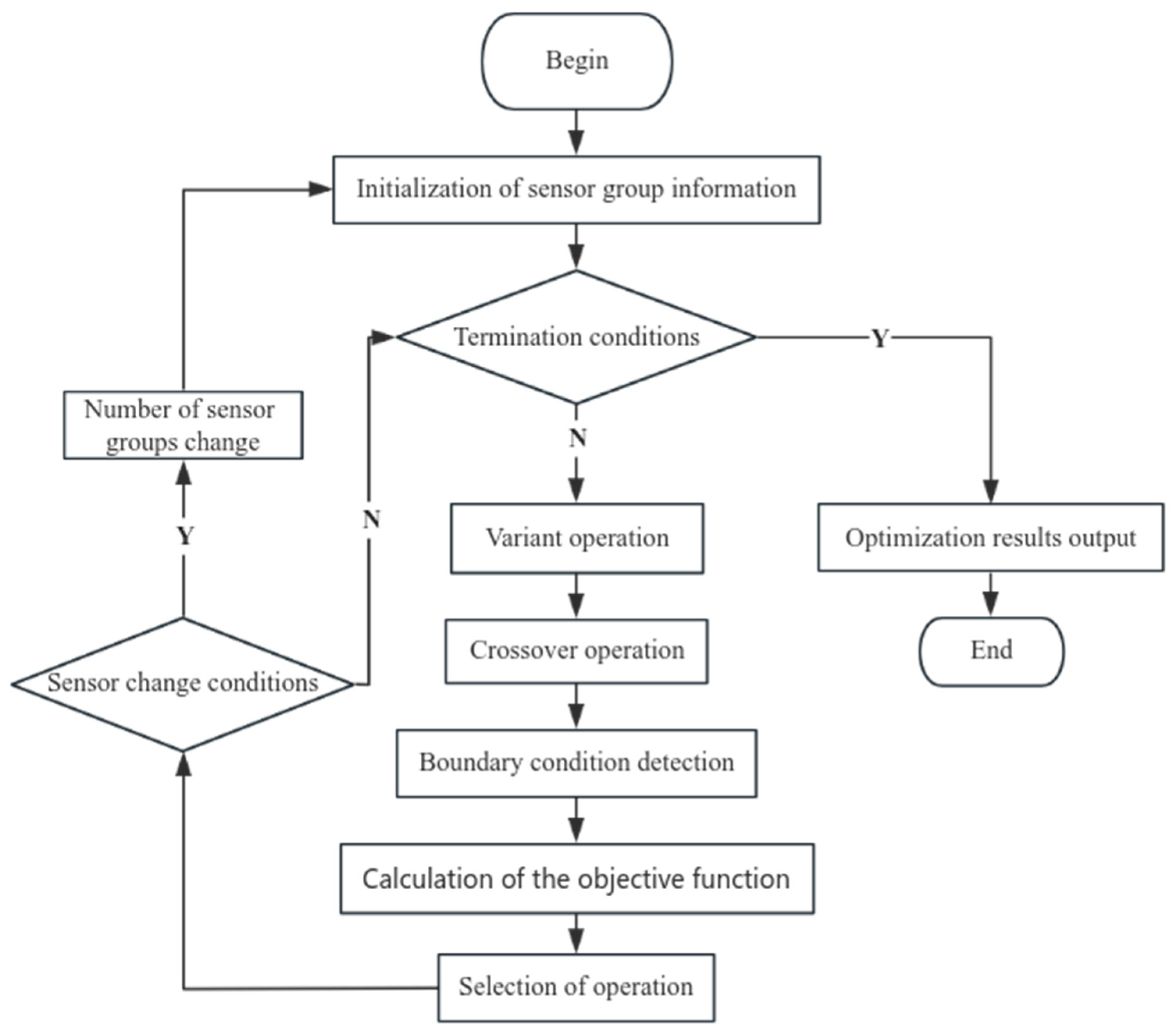
The sensor optimization algorithm is used to solve the problem of specular reflection in structured light 3D measurements. This algorithm is based on the improvement of the differential evolution algorithm [21,22,23]. The main objective of the algorithm is to optimize the sensor system and derive the number and position of projectors and cameras. The algorithm is based on an improved differential optimization algorithm that is able to quickly iterate over the optimal number and position of sensors. This algorithm is efficient for optimizing the sensor layout because it can adaptively adjust the parameters based on the number of iterations, accelerating the convergence of the results to obtain sensor data that meets expectations. The flowchart of sensor number and position optimization is shown in Figure 8.

To simplify the computational complexity, the specular reflection problem is transformed into a sensor position search problem. The initial data of the algorithm are D rows and N columns of integer-valued parameters. N denotes N sensor combinations, D denotes D sensors, and each combination contains the position information of D sensors. The initial combination is denoted by X. Then, the mutation operation is performed according to Equation (5), where i, r₁, r₂, and r₃ denote the dimensions, and r₁, r₂, and r₃ are integers that are different from each other. F is the variation operator, which is calculated by Equation (6), where F₀ is the initial “mutation” operator and G denotes the maximum number of iterations of the optimization algorithm. Next, boundary condition constraints are imposed on the variant combinations to ensure that the newly generated combinations are in the feasible domain. After comparing the objective function values of the initial combination X and the variant combination V, a crossover operation is performed. Replace the initial combination X_i with the corresponding combination in the variant combination V_i, whose function value is better than that of the initial combination X_i. Furthermore, determine whether the parameter value D needs to be changed and whether the termination condition is satisfied. If the termination condition is satisfied, the optimal combination is the output. 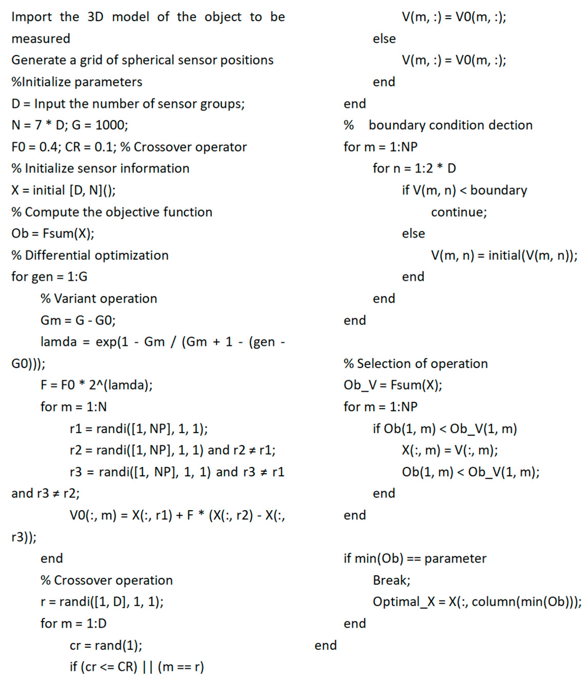The objective function value is calculated by Equation (7), where F_fein is the non-covered area and specular reflection area of the nth sensor in a sensor combination, F_sum is the non-covered area and non-specular reflection area of the combination, and the smaller F_sum is the better area. The pseudocode of the algorithm is shown in Appendix A.

$$V_i=X_{r1}+F•(X_{r2}-X_{r3})$$

(5)

$$F=F_0\ast 2^{\lambda },\lambda =e^{1-\frac{Gm}{Gm+1-G}}$$

(6)

$$F_{sum}=F_{fei1}\odot F_{fei2}\odot \cdot \cdot \cdot \odot F_{fein}$$

(7)

3. Simulation

The simulation is verified for the turbine blade body of the airplane, which is shown in Figure 4. The following approximation was used: the projector was considered a point light source, and the surface of the object was considered a complete specular reflection. Based on the light from the projector, the characteristics of the surface of the object under test, and the pointing of the camera, the possible specular reflection areas in a set of sensors are predicted. The relevant parameters optimized by the simulation are shown in

Table 1. Experimental device parameters.

Blade Size (mm)	Blade Material	Distance (Projector and Object) (mm)	Distance (Projector and Camera) (mm)
53 × 58 × 205	Titanium	900	170

. The hardware processor used in this simulation is the Intel (R) Core (TM) i5-4590 CPU @ 3.30 GHz; the Windows version used is Windows 10 Professional Edition; the simulation software used is Matlab R2022a; and the verification software used is 3Dmax 2020.

Based on these parameters and the 3D data of the object, specular reflection region prediction is performed. The performance of the sensor combination is also evaluated through simulation verification. This helps to optimize the sensor configuration, enabling accurate measurement data to be obtained for 3D structured light measurements, as well as providing strong support for the analysis and design of the turbine blade body. The optimal sensor set coverage obtained after sensor system optimization is shown below:

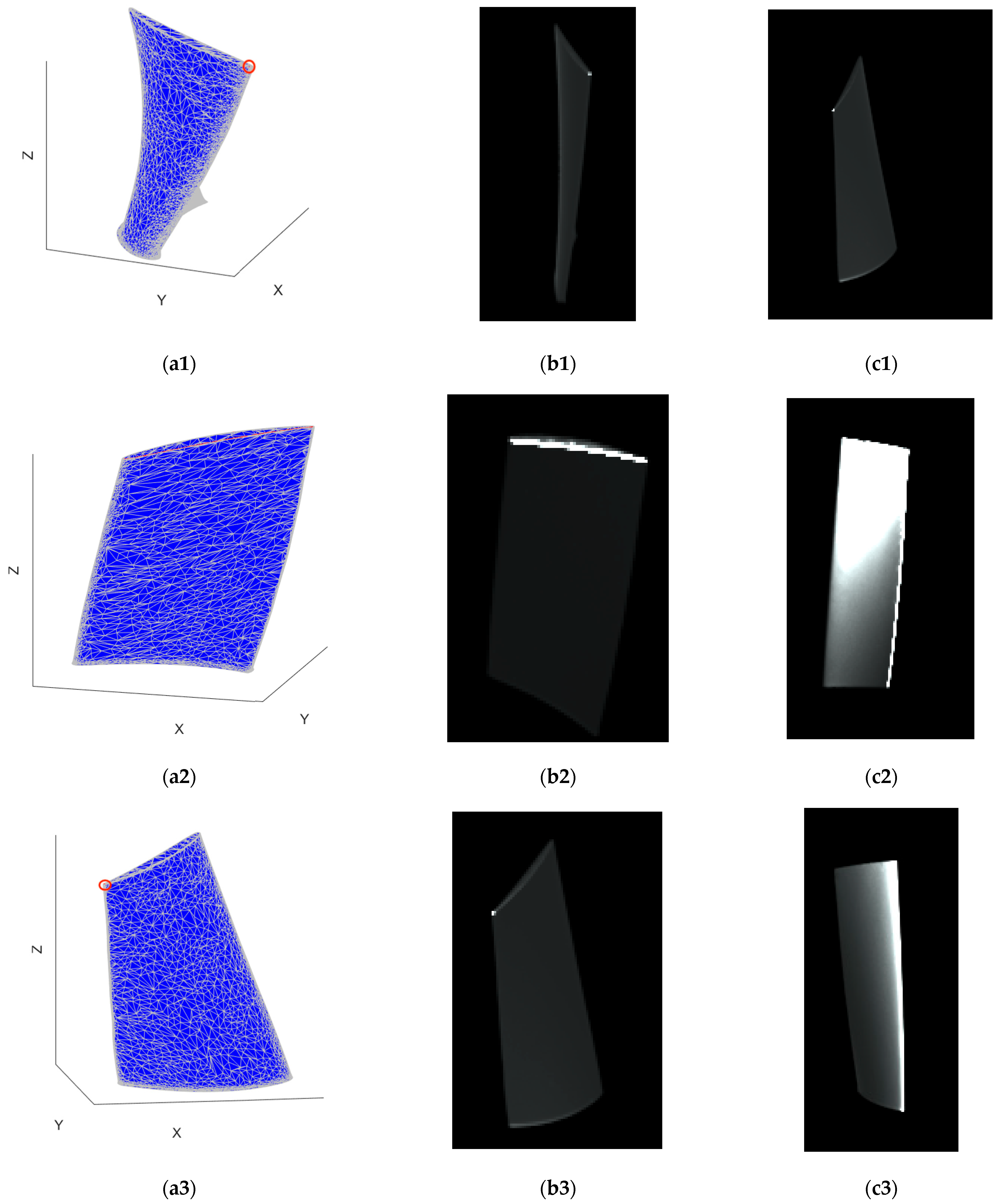
Figure 9 shows the optimization results of the algorithm and the validation of the specular reflection area. There are three images in Figure 9a1–a3, and the result of sensor optimization is that only three pairs of sensors are needed to cover the measurement surface at once. The black areas in Figure 9a1–a3, represent the covered areas of the three sets of sensors. The red area is the specular reflection area. Due to the small specular reflection areas in Figure 9a1,a3, we used a red circle to indicate the specular reflection area. By comparing the red areas in the three photos, it can be seen that the specular reflection areas within the coverage areas of the three sets of sensors are different. By comparing the black areas, it can be seen that there is overlap in the coverage areas of the three sets of sensors. By comparing the red and black parts, it can be seen that the specular reflection area of one set of sensors is the non-specular reflection area in the coverage area of another set of sensors. The non-highlight coverage area of three sets of sensors covers the measurement surface of the object. Therefore, from the overall perspective of the three sets of sensors, the problem of specular reflection has been solved, and Figure 9b1–b3 is a specular reflection area validation by 3Dmax. The highlighted white areas in Figure 9b1–b3 are the specular reflection areas calculated by 3Dmax. By comparing the results of groups Figure 9b1–b3,c1–c3, it can be verified that the specular reflection area calculated by the optimization algorithm is accurate. Hence, it also proves that the sensors optimized by the optimization algorithm can cover the measurement area while solving the specular reflection problem.

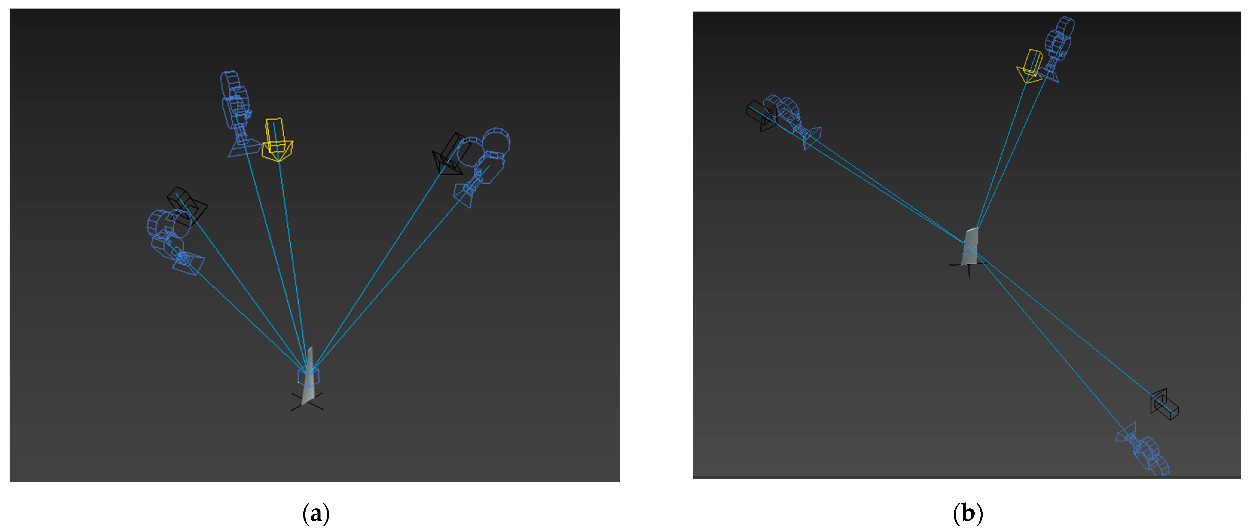
Figure 10a is a schematic diagram of sensor positions optimized by the algorithm. Figure 10b is a schematic diagram of sensor positions optimized by the expert. Figure 9c1–c3 is an optimization diagram of the number and location of sensors manually selected by experts. Artificial intelligence generally tends to place sensors directly in front, behind, or above objects, and the algorithm can consider more sensor positions than manual labor. From the sensor coverage area in Figure 9, it can be seen that the optimization results of the algorithm are better than those of manual methods. When manually optimizing the number and location of sensors, it requires a significant amount of time. Moreover, the optimized results may not be the best. When a large number of sensors are required, the efficiency of manual optimization is much lower than that of algorithms. Hence, the algorithm proposed in this article improves the efficiency of optimizing the number and position of sensors.

4. Conclusions

For the problem of specular reflection in three-dimensional measurement, this paper proposes a sensor optimization algorithm. The algorithm optimizes the number and pose of sensors in the measurement system. The goal of optimization is to minimize the number of sensors as much as possible while avoiding the impact of specular reflection. It can improve the efficiency of determining sensor coverage areas and reduce subsequent measurement costs. First, the specular reflection problem is viewed as a multi-sensor position search problem. Then, an optimization algorithm is used to find the optimal number and bit positions of sensors to avoid specular reflection. Experiments show that the best multi-sensor system obtained by the algorithm improves the model coverage rate and solves the specular reflection problem.

This article optimizes the sensor for measuring turbine blades. The result of algorithm optimization is that three sets of sensors can cover the overall measurement area of the blade while solving the problem of specular reflection. This algorithm minimizes the number of sensors as much as possible while ensuring that the sensor’s field of view covers the measurement area. This algorithm achieves automated matching of multiple sensor coverage areas, highlight areas, and object measurement areas, saving time and improving efficiency.

We believe that future work should include the following aspects: (1) optimizing the structure of algorithms and improving their operational efficiency; (2) considering large objects as measurement objects and optimizing the sensors; and (3) writing an optimization software based on algorithms.