1. Introduction and Related Research
Indoor positioning has garnered significant attention in recent years due to its critical role in applications such as autonomous navigation, robotics, and smart environments. Unlike outdoor positioning systems, such as Global Positioning System (GPS), which suffer from signal attenuation and multipath effects indoors, indoor positioning requires alternative solutions. Existing indoor positioning technologies can be broadly categorized into magnetic, inertial, acoustic, optical, radio frequency (RF), and vision-based approaches, as shown in
Table 1.
Magnetic-based positioning determines location by analyzing perturbations in the Earth’s magnetic field or magnetic materials. This technique exhibits high robustness for indoor fingerprinting. However, sensor-dependent variability can lead to inconsistent results [
1,
2,
3]. Inertial methods utilize accelerometers and gyroscopes to infer movement and orientation without relying on external infrastructure. This feature makes them ideal for GPS-denied environments. These systems often suffer from cumulative errors and sensor drift over time [
4]. Acoustic methods leverage characteristics such as time delay and signal attenuation to estimate distance. These systems are suitable for low-light or visually complex environments. However, signal attenuation over long distances or obstacles can present challenges [
5].
Optical positioning technologies employ infrared or visible light signals to estimate target locations. While capable of achieving high precision, they are sensitive to lighting variations, occlusion, and reflective surfaces [
6]. RF-based systems included Wi-Fi, Bluetooth low energy (BLE), radio frequency identification (RFID), and ultra-wideband (UWB). They are well-suited to complex indoor scenarios due to their ability to penetrate walls and obstacles. Vision-based positioning uses fixed or mobile cameras to extract spatial features from nature environment. Although they can provide high-resolution spatial information, these systems tend to be computationally intensive and often fail under poor lighting conditions [
7].
In addition to localization, vision-based obstacle recognition plays a pivotal role in applications such as autonomous driving, drone navigation [
8], and railway safety systems [
9]. Current monocular vision-based obstacle detection techniques are generally divided into two categories: feature-based and motion-based methods. Feature-based approaches extract visual characteristics such as color, shape, texture, or edges to detect and classify obstacles. Machine learning algorithms, including neural networks and support vector machines (SVMs), have further improved obstacle classification performance by learning from large datasets. However, these models often struggle with occluded or distant objects and unfamiliar obstacle types. On the other hand, motion-based approaches such as background subtraction, optical flow analysis, and inter-frame differencing are effective in dynamic environments but typically provide only two-dimensional localization and suffer from limited depth perception, especially over greater distances.
Indoor positioning and obstacle recognition, though traditionally studied as separate research areas, share numerous technical challenges and environmental constraints. Both require reliable operation in complex, dynamic indoor settings and depend heavily on visual feature extraction, particularly in the absence of external signals such as GPS or RF. Indoor positioning focuses on global positioning, while obstacle recognition emphasizes local awareness. However, both must be robust to occlusion, lighting changes, and material reflections. Recent advances in texture-based methods such as LBP and FFT have demonstrated cross-domain applicability, enhancing both positioning accuracy and object discrimination. The IMU module, which includes an accelerometer, gyroscope, and magnetometer, provides acceleration, angular velocity, and magnetic field data. This fusion enhances system performance under low-light, occluded, or visually degraded environments. Moreover, inertial-visual fusion techniques help mitigate sensor drift in localization while reducing noise and motion blur in recognition tasks. These shared requirements and synergistic techniques motivate the development of unified algorithms that can serve both functions.
In our earlier work, we introduced the LRA, which establishes a logarithmic relationship between the laser irradiated area of spots and actual distance [
10]. Experimental results demonstrated a minimum error of 1.6 cm and an average error of 2.4 cm within a 3 m range. However, since the algorithm only leverages local features from images, it lacks the capability to differentiate between background surfaces and actual obstacles, especially when material reflectivity varies under different lighting conditions.
To improve recognition accuracy, we developed the LBP-CNNs model [
11], which integrates LBP with CNNs. LBP is a widely adopted texture descriptor with rotation and grayscale invariance that can efficiently extract local texture features. This design not only reduces computational cost but also retains key image characteristics. The experimental results showed that the LBP-CNNs model achieved an average ranging error of 1.27 cm and an obstacle recognition accuracy of 92.3%.
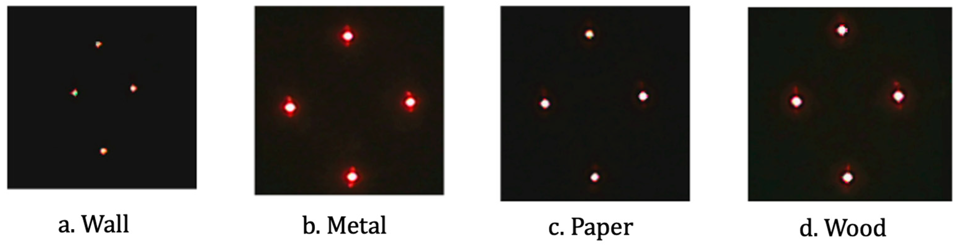
To further investigate this limitation, we conducted experiments evaluating laser reflections on surfaces made of different materials. As shown in
Figure 1, the reflection intensity of the laser spots varied significantly across wall, metal, paper, and wood surfaces. Notably, obstacles (e.g., metal or wood) produced more prominent and consistent reflections compared to flat background walls. These findings confirmed that surface material characteristics and illumination angle play a critical role in visual-based ranging performance and motivated the development of more robust feature extraction and classification methods.
In addition, we extended the LBP-CNNs architecture by integrating FFTs, resulting in the LBP-FFT-CNNs model. FFT converts image data from the spatial domain to the frequency domain and extracts the parts that are critical for identifying textures, edges, and repeating patterns. This transformation improves the ability of feature discrimination, reduces the data dimension, and improves the classification efficiency. Experimental evaluations demonstrated a recognition accuracy of 98.6%, with average indoor positioning errors reduced to 0.91 cm. The key contributions of this paper are summarized as follows:
Device Optimization: We improved the original MC4L design by integrating an IMU module to form the MC4L-IMU device, thereby increasing adaptability in complex indoor environments.
Obstacle Recognition Accuracy: By introducing FFT-based feature extraction, we significantly reduced computational overhead while improving recognition accuracy to 96.3%.
Model Efficiency: The proposed LBP-FFT-CNNs model features a simplified architecture with consistently low prediction standard index (PSI) values (<0.02), indicating high robustness.
Hybrid Positioning Algorithm: We developed an inertial-visual fusion algorithm that achieves sub-centimeter positioning accuracy, even in low-light environments.
The remainder of this paper is structured as follows:
Section 2 describes the module structure and provides a connection diagram for the MC4L-IMU device.
Section 3 introduces the proposed LBP-FFT-CNNs model and detail processing pipeline.
Section 4 describes the experimental environment and fusion-based indoor positioning algorithm.
Section 5 provides a comprehensive performance evaluation, including regression and classification metrics, and a discussion of the experimental results. Finally,
Section 6 summarizes our conclusions and outlines future research directions.
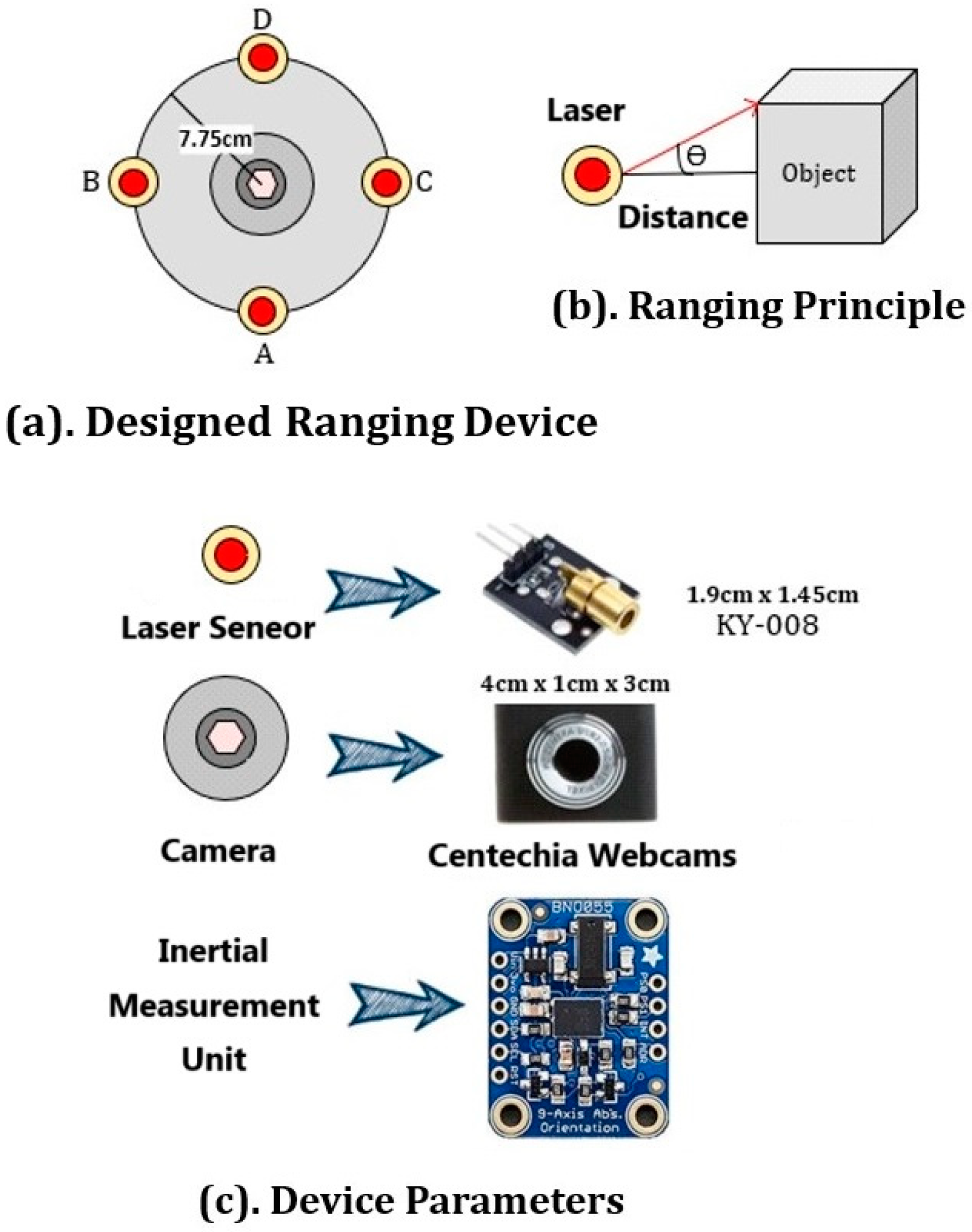
2. Structure and Connectivity of the MC4L-IMU Device
To accurately detect the motion state and directional changes of a target object, we designed a circular structured vision-based ranging system. The system consists of four KY-008 laser transmitters, which are evenly distributed along a circular orbit with a radius of 7.7 cm. A standard high-definition monocular camera is placed at the center of the orbit, ensuring that the laser projections form consistent geometric patterns on the target surface. The choice of a circular laser arrangement improves depth perception and range accuracy through triangulation and irradiated area estimation, as supported in prior visual-laser fusion systems [
12,
13]. All sensors and components are connected to a Raspberry Pi 4 Model B (4 GB RAM), which serves as the control and data processing unit. The Raspberry Pi platform is widely used in embedded vision systems due to its low power consumption, integrated I/O interfaces, and sufficient computational capability for lightweight image processing tasks [
14].
The target object was positioned at an initial distance of 120 cm, and measurements were conducted every 5 cm until a maximum distance of 300 cm was reached. All images were captured at a resolution of 640 × 480 pixels, a commonly adopted setting in monocular vision research for balancing image detail and computational cost [
15].
Furthermore, to reduce the impact of ambient light and ensure consistent illumination conditions, all experiments were conducted in a dark environment. Each distance point was measured three times to account for variability and improve the statistical robustness of the dataset.
Figure 2 shows the structure of the MC4L-IMU device.
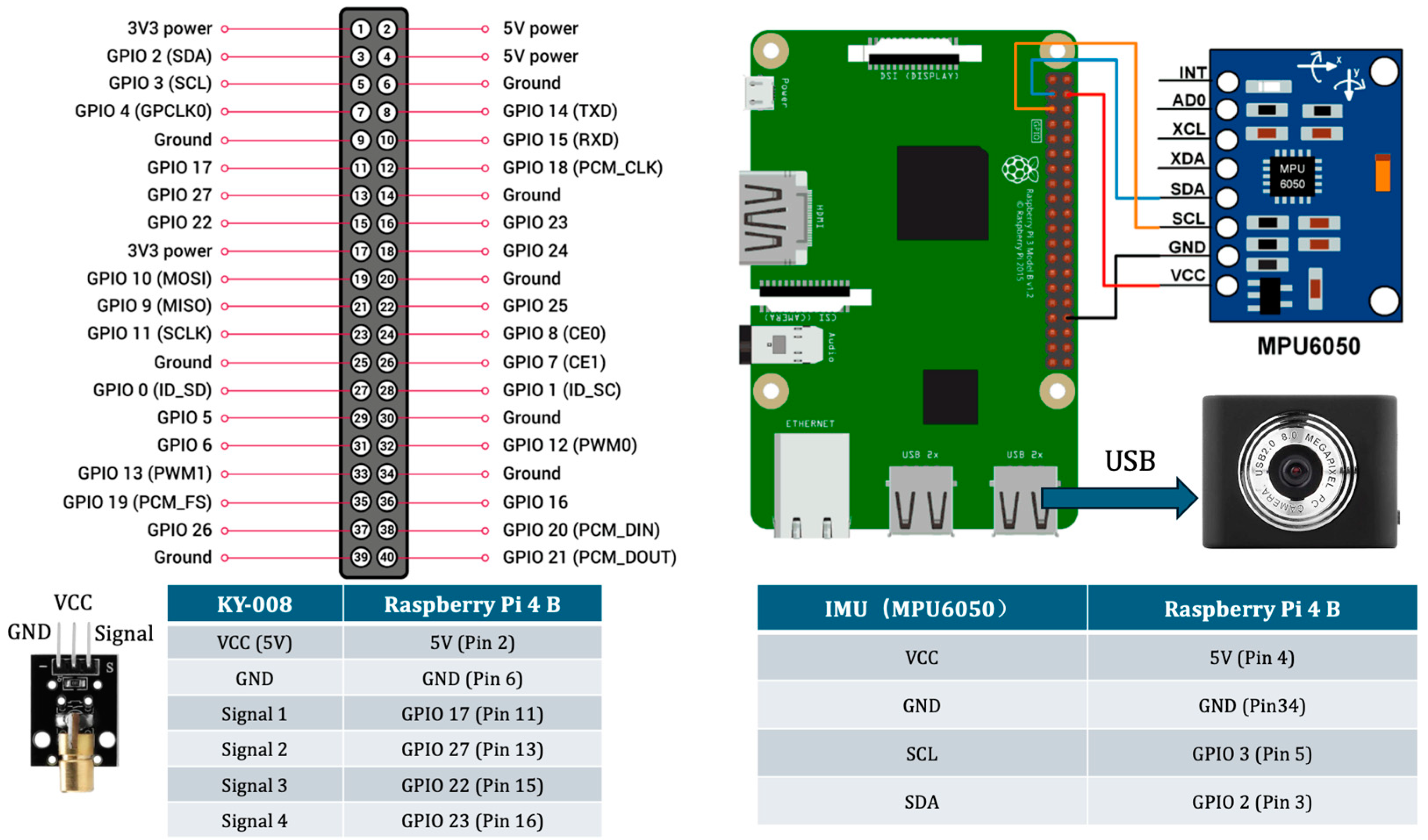
We employed a Raspberry Pi 4B as the core processing unit, interfacing it with a KY-008 laser module, an MPU6050 IMU, and a USB camera to establish a comprehensive sensing system. The KY-008 laser module was connected via the GPIO interface, with four signal lines assigned to distinct GPIO pins for precise control over laser activation. The MPU6050 IMU sensor utilized an I2C communication protocol, with GPIO 2 (SDA) and GPIO 3 (SCL) facilitating motion tracking and orientation estimation. A USB camera, serving as the primary vision sensor, was linked through a standard USB port to enable real-time image acquisition and processing.
Figure 3 shows Integration of different sensors for the MC4L-IMU device. To ensure system stability and reliable operation, appropriate power connections were configured, maintaining a 5 V power supply and proper grounding. A detailed pin mapping of sensor connections to Raspberry Pi is provided for clarity and ease of implementation.
3. The LBP-FFT-CNNs Model
3.1. Architecture of the LBP-FFT-CNNs Model
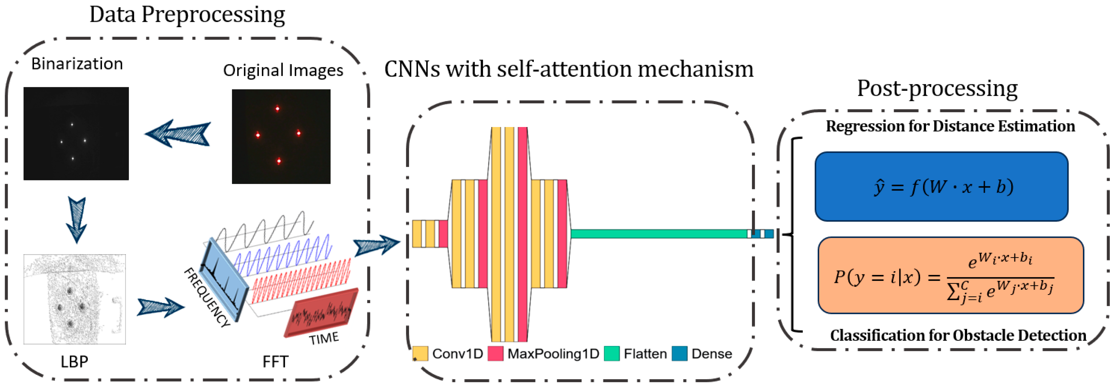
The LBP-FFT-CNNs model is divided into three components: data preprocessing, CNNs with a self-attention mechanism, and post-processing. The post-processing stage encompasses two tasks: regression for distance estimation and binary classification for obstacle recognition.
Figure 4 illustrates the architecture of the LBP-FFT-CNNs model.
In the data preprocessing step, original images are first binarized, simplifying them into black-and-white information to reduce computational complexity while retaining essential visual features. The LBP is utilized to extract texture features from images, enhancing the representation of local details. Additionally, the FFT is applied to convert the images from spatial domain to frequency domain, enabling the model to analyze frequency characteristics and effectively detect periodic patterns.
The preprocessed data are then input into a one-dimensional Convolutional layer (Conv1D) for feature extraction, where convolution operations efficiently capture local patterns. To reduce computational overhead and retain significant feature information, a max pooling layer (MaxPooling1D) is employed for down sampling the extracted features. Subsequently, a flatten layer is used to transform multi-dimensional features into a one-dimensional vector, facilitating further processing in fully connected layers.
During the feature extraction process, a self-attention mechanism is introduced to enhance the model’s ability to understand global information and capture key features more effectively. Finally, the network output serves two purposes: first, regression is performed to estimate the distance to the object; second, a classification model is applied for obstacle detection, using a SoftMax function to predict the probability of input belonging to different obstacle categories. This multi-task learning framework enables simultaneous distance estimation and obstacle recognition, significantly enhancing the model’s practicality and efficiency.
The CNNs has a total of eight Conv1D layers, and each two Conv1D is a group. Conv1D is a 1D convolution operation that extracts features at different levels by scanning filters on input data using a sliding window. Each group is followed by a MaxPooling1D. MaxPooling1D is a down sampling operation used to reduce the dimensionality and computational complexity of feature maps. It selects the maximum value on each sliding window of 1D data and takes these maximum values as output. The activation function uses ReLU. Then, the flatten function is used to convert the 2D data into 1D data. It converts multi-dimensional data into a 1D form and maintains the order of all elements. The number of neurons in fully connected layer is 10 using the dense function provided by the Keras library [
16].
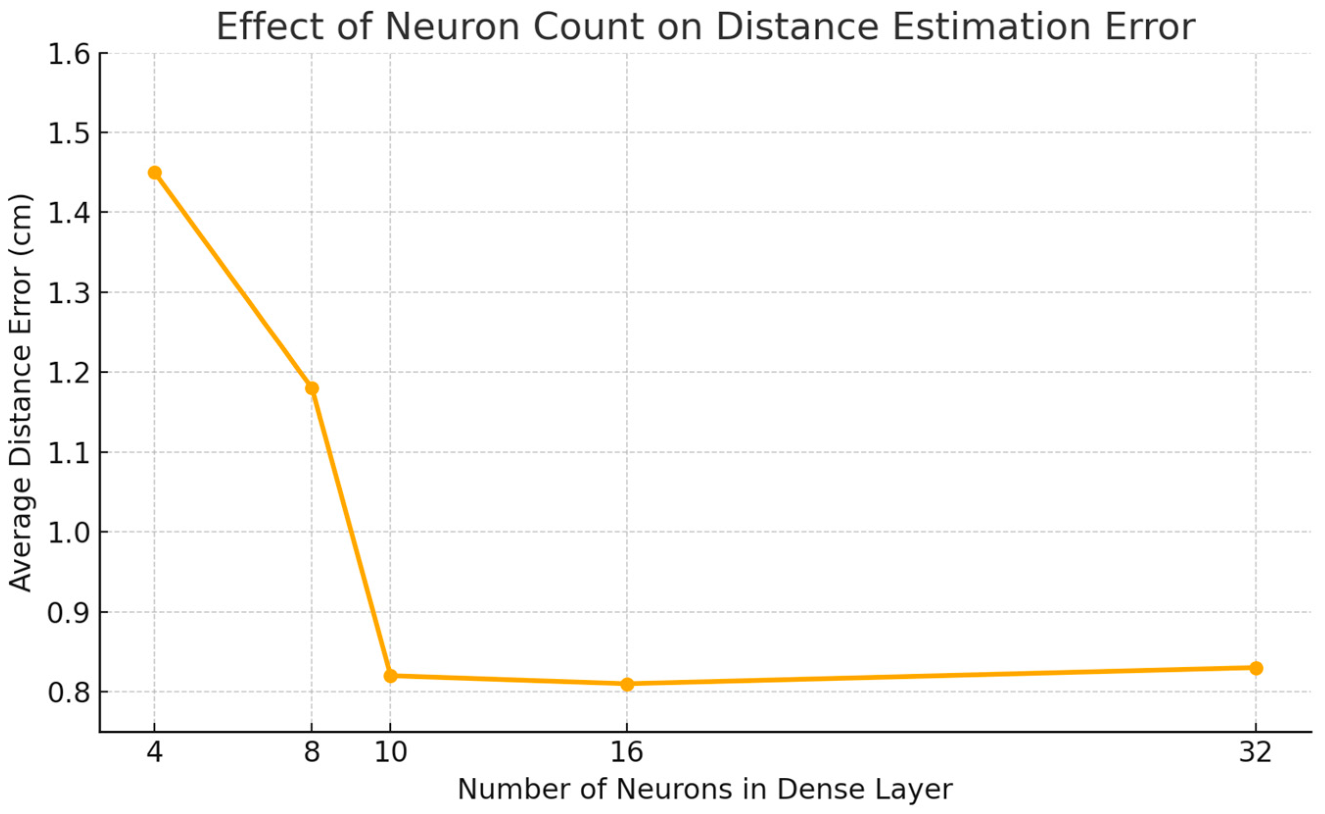
Figure 5 illustrates the performance of the LBP-FFT-CNNs model under varying numbers of neurons in the final dense layer. Increasing the number of neurons in the dense layer significantly improves the distance estimation accuracy, with the lowest error of 0.81 cm achieved at 16 neurons. However, further increasing the count to 32 does not yield additional benefits and slightly increases the error. Overall, a configuration of 10–16 neurons provide the best balance between performance and computational efficiency. Considering the computational cost on embedded devices and the fact that our dataset includes obstacle samples from ten different material types, we ultimately selected a 10-neuron configuration to ensure robustness and real-time feasibility.
3.2. Computational Complexity Analysis
While the integration of FFT and self-attention mechanisms enhances feature representation and model robustness, it inevitably introduces additional computational overhead. FFT transforms spatial image data into the frequency domain, which involves operations per image, where is the number of pixels. However, due to selective frequency component retention, the overall dimensionality is reduced before entering the convolutional layers, partially offsetting the added cost.
The self-attention module, designed to capture global dependencies across feature maps, requires time and space complexity for feature maps of size . While more computationally demanding than standard convolution, its inclusion significantly improves the model’s ability to distinguish between background textures and obstacles under challenging conditions.
To ensure practical feasibility, we apply both FFT and self-attention only at specific stages in the network. Additionally, experiments were conducted on a Raspberry Pi 4 platform to validate real-time performance, confirming that the processing speed remains acceptable for embedded applications in indoor positioning.
3.3. Data Preprocessing
3.3.1. A Binarization Process Based on the Adaptive Threshold
Image binarization is the process of converting a grayscale image into a black-and-white representation by setting pixel values to either 0 or 255. This transformation is based on an adaptive threshold , as shown in Equation (1). If a pixel’s value exceeds the threshold , it is set to white (255); otherwise, it is set to black (0). Here, represents the input image, and represents the resulting binarized image.
In Equations (2) and (3), denotes the threshold value at pixel location in the image, while represents the grayscale value of images at that pixel. The parameter block size, denoted as , specifies the size of local region used for threshold determination, and is a constant that adjusts computed threshold.
Adaptive thresholding [
17,
18] determines threshold value based on the statistical characteristics of local image regions. This method offers superior adaptability to variations in lighting conditions and noise distributions across different areas of images. Moreover, it helps preserve image details while minimizing information loss during the binarization process.
3.3.2. The Circular Local Binary Pattern Operator
The Circular Local Binary Pattern (CLBP) [
19] operator extends the concept of LBP by incorporating circular neighborhoods, which can capture texture information more effectively. Let
denote the grayscale intensity of pixel at coordinates
. Define a circular neighborhood around center pixel
with radius
. The circular neighborhood consists of
points equally spaced around a circle of radius
centered at
. These points can be represented as
for
i as follows:
where
ranges from 0 to
, and
represents the coordinates of
i-th point in circular neighborhood. For each pixel
, compute the
value
as shown in Equation (5).
where
is defined as follows:
Here, represents the intensity value of i-th point in circular neighborhood, and is the intensity value of center pixel.
3.3.3. FFT
FFT [
20] converts texture information from the spatial domain to the frequency domain, emphasizing distinct frequency components of texture. It provides additional discriminative features for LBP-CNNs by capturing these subtle differences. Furthermore, combining LBP-based spatial patterns with frequency characteristics significantly enhances the network’s ability to recognize unique patterns, and even spatial texture differences are minimal or nearly indistinguishable. FFT also effectively filters out high-frequency noise or irrelevant low-frequency components, focusing on the most informative frequency bands. This capability strengthens the robustness of LBP-CNNs against variations in lighting, shadows, or environmental conditions that often affect texture representation and make distinguishing similar textures more challenging. Suppose the FFT transforms a spatial domain texture
into its frequency domain representation
. The FFT of this sequence is defined as follows:
where
and
represent spatial coordinates and frequency coordinates, respectively.
and
are dimensions of the texture image.
is the imaging unit. This transform decomposes texture into its frequency components where magnitude
represents the strength of a frequency and phase. Here,
encodes spatial alignment. Obstacles with similar textures in the spatial domain may differ in their frequency domain representations. FFT highlights these differences as follows:
where
and
are the frequency domain representations of two textures. Even if spatial patterns are similar,
due to variations in high- or low-frequency components. Combining spatial features
(captured by LBP) with frequency features
augments the feature space as follows:
where
act as weights to balance spatial and frequency contributions. This dual domain feature improves the discriminative power of LBP-CNNs. The FFT allows filtering of noise by zeroing out specific frequency bands. For instance, it applies a low-pass filter to filter high-frequency noise:
where
CF is the cutoff frequency. This operation enhances the signal-to-noise ratio, making the textures more distinguishable under varying conditions. The combined spatial and frequency features are fed into the CNNs, which learns discriminative mappings
during training:
is the predicted label of obstacle, and is the trainable parameters of the CNN.
3.4. CNNs with a Self-Attention Mechanism
To allow CNNs to dynamically pay attention to information at different locations when processing input data, we introduce a self-attention mechanism [
21] in hidden layers. In the self-attention mechanism, we first multiply input tensor
by three weight matrices
,
, and
to obtain
,
, and
tensors. These tensors are used to calculate attention scores and weighted values as shown in Equation (12):
where
,
, and
represent the
information,
information, and
information of the current location. The
tensor represents the correlation between
and
, which determines the importance of each position when calculating weighted value. The calculation method is to divide the inner product of
and
using a scaling factor
and then normalize it using the SoftMax function shown in Equation (13).
Here,
denotes the dimensionality of the key vectors. The scaling factor
is used to prevent large dot product values, which can cause gradients to become too small during the SoftMax operation. This normalization improves train stability and convergence. Once attention scores are computed, they are used to weight the value vectors
. The weighted sum of these values produces the output of self-attention layer.
Finally, the obtained weighted value is multiplied by another weight matrix to obtain the final output layer. The integration of LBP with a self-attention mechanism leverages the local texture encoding capability of LBP and global contextual analysis strength of self-attention, resulting in a more comprehensive feature representation. The self-attention mechanism compensates for LBP’s limitations in distinguishing complex scenes or similar textures by focusing on critical regions. This combination enhances model’s robustness, computational efficiency, and generalization ability, leading to superior performance in texture analysis tasks.
3.5. Post-Processing
In this section, our post-processing is mainly divided into regression and classification. Regression is used to predict the measured distance; classification is used to determine whether front is an obstacle or a wall.
3.5.1. Regression for Distance Estimation
For regression problems, the output layer is usually a single node or multiple nodes that predict continuous values. Since we want to predict a single continuous value, the formula of output layer can be described as follows:
where
is output of model.
is weight, and
is the input feature vectors.
is bias, and
is identity function.
3.5.2. Classification for Obstacle Detection
We use the SoftMax function as an activation function because it converts raw output of neural network into a probability distribution for class predictions as shown in Equation (18).
where
is the predicted probability of class
given input
.
is the total number of class and set to 2.
are the weight and bias of
i-th class, respectively. During training, we adopt the cross-entropy loss function to measure differences between predicted values and true labels.
4. An Indoor Positioning Algorithm Combining IMU and LBP-FFT-CNNs
4.1. Inertial-Based Positioning Algorithm Using IMU
IMU provides measurements of acceleration and angular velocity in three-dimensional space. The inertial-based positioning algorithm computes position, velocity, and orientation by integrating these measurements over time. It is divided into the five following steps.
4.1.1. Sensor Data Acquisition
The IMU provides raw acceleration and angular velocity data at regular intervals.
4.1.2. Orientation Estimation
Orientation
is computed using an extended Kalman filter (EKF) [
22] fusion algorithm by integrating angular velocity:
where
is angular velocity vector over time. This determines the orientation of sensor frames relative to a global frame.
4.1.3. Gravity Compensation
The measured acceleration includes both linear acceleration
and gravitational acceleration
. Gravity is removed to compute linear acceleration:
where
is a gravity vector, typically derived from orientation information.
4.1.4. Double Integration for Position
Velocity
is obtained by integrating linear acceleration, where
is initial velocity:
Position
is determined by integrating the velocity, where
is initial position:
4.1.5. Sensor Data Dynamic Fusion Based on the EKF Algorithm
The integration of two systems is demonstrated using the EKF algorithm as follows:
where
is the Kalman filter. The LBP-FFT-CNNs model performs obstacle detection and classification by analyzing visual texture and frequency information. Integrating it with IMU data addresses the limitations of each system, resulting in a more robust positioning and obstacle detection framework. First, the LBP-FFT-CNNs model provides absolute position updates or corrections using visual feature matching, mitigating drift. Second, IMU data offer high-frequency updates, complementing the relatively slower processing speed of vision system to ensure real-time tracking and positioning. The third aspect lies in adaptability to diverse environments, enabling efficient performance in both feature-rich and feature-scarce scenarios.
4.1.6. EKF Derivation and Parameter Settings
The EKF is applied in this work to fuse inertial and visual positioning data. The algorithm follows the standard predict–update structure based on a nonlinear system model.
The state vector is expressed as follows:
where
is position,
is velocity, and
is orientation.
The prediction step involves the following:
where
represents nonlinear motion model based on IMU data,
is the Jacobian of
, and
is the process noise covariance.
In the update step, the visual position
is used as the measurement:
where
and
is the nonlinear measurement function. In our system,
is diagonal matrix with variances from accelerometer and gyroscope noise models.
is observation noise covariance that is estimated based on vision-based position measurement variance. The Kalman gain
in Equation (27) corresponds to the standard EKF update. This fusion ensures that the short-term accuracy of visual measurements and the high-frequency continuity of IMU data are combined.
4.2. Experimental Environment
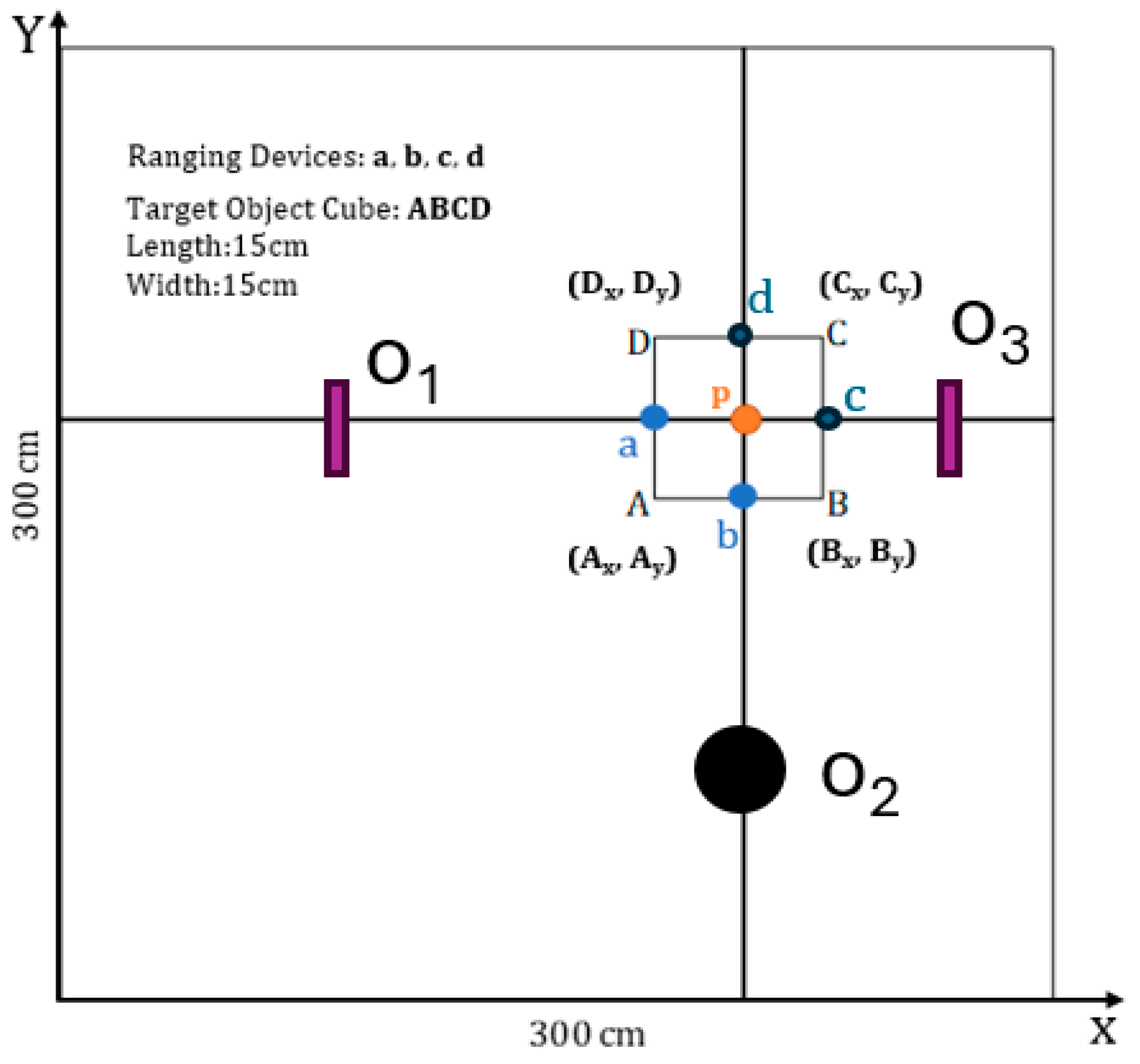
A target object cube, denoted as
, with dimensions of 15 cm × 15 cm × 15 cm, was randomly positioned within a controlled 3 m × 3 m dark environment.
Figure 6 presents a 2D schematic of the experimental environment. Since the proposed algorithm can autonomously distinguish between obstacles and walls, four devices (a, b, c, and d) were affixed to the surface of the
cube for accurate measurements. For each of 130 consecutive positions, spaced at 5 cm intervals, we conducted five measurements and compared predicted results with actual distances to compute the mean error. We chose 130 positions combinations to ensure data diversity while controlling experimental overhead. The combinations cover a variety of materials (such as metal, wood, paper, and wall), with distances ranging from 0.3 to 3 m, a step size of 5 cm, and different obstacle placements to simulate real indoor scenes. Preliminary experiments show that further increasing the number of samples has limited improvement in model accuracy (<0.2%), but training time increases significantly. Therefore, 130 is a reasonable choice that considers both representativeness and efficiency. During five imaging sessions at each position, obstacles
,
, and
were randomly placed in front of target object. Consequently, the dataset comprised 130 obstacle-present images and 520 obstacle-absent images. Each image is 640 × 480 pixels. To further assess positioning accuracy in complex environments, obstacles
,
, and
were designed with varying material properties to evaluate the system’s robustness against differences in laser beam reflections.
4.3. Indoor Positioning Algorithm Based on IMU and LBP-FFT-CNNs
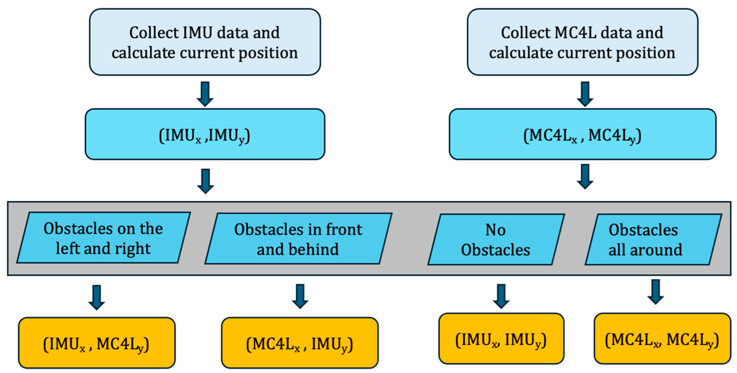
Indoor positioning algorithms need to consider both the IMU module and the vision-based computing module. Algorithm 1 illustrates an indoor positioning algorithm based on an IMU and LBP-FFT-CNNs, designed to determine the position of a target object by integrating IMU and visual data. The input includes initial position, velocity, acceleration, orientation, and time step (), while the output is the final position of the target object.
The algorithm features key sub-functions: retrieves acceleration and angular velocity data from the accelerometer and gyroscope, updates the object’s orientation based on angular velocity and time step, calculates updated velocity using acceleration and time step, and computes the new position based on updated velocity and time step.
In the main loop, IMU data are acquired, followed by sequential updates to orientation, velocity, and position. After updating orientation, acceleration is transformed into a global coordinate system for improved accuracy. The final position is determined through conditional checks. If obstacles are detected on the left or right, the algorithm combines IMU-derived x-coordinates and visual y-coordinates. Similarly, for obstacles above or below, the algorithm uses visual x-coordinates and IMU-derived y-coordinates. If surrounded by obstacles, both coordinates are derived from IMU data; otherwise, both are based on visual data.
In summary, the algorithm integrates IMU and visual data to accurately determine the object’s position, especially under obstacle interference, ensuring reliable positioning.
Figure 7 shows the flow chart of the positioning algorithm combining IMU and LBP-FFT-CNNs.
| Algorithm 1. Inertia-based Indoor Positioning Algorithm based on LBP-FFT-CNNs |
Input: position, velocity, acceleration, orientation and time_step = Δt
Output: Target object position |
| 1 | Define function get_IMU_data(): |
| 2 | acceleration = read_accelerometer() |
| 3 | angular_velocity = read_gyroscope() |
| 4 | return acceleration, angular_velocity |
| 5 | Define function update_orientation(orientation, angular_velocity, Δt): |
| 6 | orientation = orientation + angular_velocity * Δt |
| 7 | return orientation |
| 8 | Define function update_velocity(velocity, acceleration, Δt): |
| 9 | velocity = velocity + acceleration * Δt |
| 10 | return velocity |
| 11 | Define function update_position(position, velocity, Δt): |
| 12 | position = position + velocity * Δt |
| 13 | return position |
| 14 | while True: |
| 15 | acceleration, angular_velocity = get_IMU_data() |
| 16 | orientation = update_orientation(orientation, angular_velocity, time_step) |
| 17 | global_acceleration = convert_to_global_frame(acceleration, orientation) |
| 18 | velocity = update_velocity(velocity, global_acceleration, time_step) |
| 19 | IMU_position = update_position(position, velocity, time_step) |
| 20 | if obstacles on the left or right sides of object are TRUE: |
| 21 | vision_position_y = (C_y − B_y)/2 + B_y |
| 22 | return (IMU_position_x, vision_position_y) |
| 23 | Else if obstacles above or below the object are TRUE: |
| 24 | vision_position_x = (C_x − B_x)/2 + B_x |
| 25 | return (vision_position_x, IMU_position_y) |
| 26 | Else if obstacles surround the object are TRUE: |
| 27 | return (IMU_position_x, IMU_position_y) |
| 28 | Else if no obstacles around the object are TRUE: |
| 29 | return (vision_position_x, vision_position_y) |
5. Performance Evaluation
5.1. Performance Evaluation Methods
We calculate the positioning error using Euclidean distance, as defined by the following:
where
is the predicted position, and
is the actual position of objects. A determination coefficient is usually utilized to measure the fitting degree of a regression model and expressed as
. It can be calculated using the following equation:
where
(residual sum of squares) represents the sum of squares of the difference between model predictions and actual observations.
(total sum of squares) represents the sum of squares differences between predicted variables and its meaning. The value of
ranges from 0 to 1. The closer it is to 1, the better the model fits the data. In contrast, the closer it is to 0, the worse the model fits the data.
Figure 8 shows the determination coefficients of LRA, LBP_CNNs, and LBP_FFT_CNNs under 10 random distances. The results reveal that LRA achieves an
of 0.9867, demonstrating robust performance but falling short compared to deep learning-based models. LBP_CNNs, with a
of 0.9934, exhibits superior capability in capturing intricate data patterns. Notably, the LBP_FFT_CNNs model attains the highest
of 0.9949, underscoring the efficacy of integrating Fourier-transformed features into convolutional neural networks.
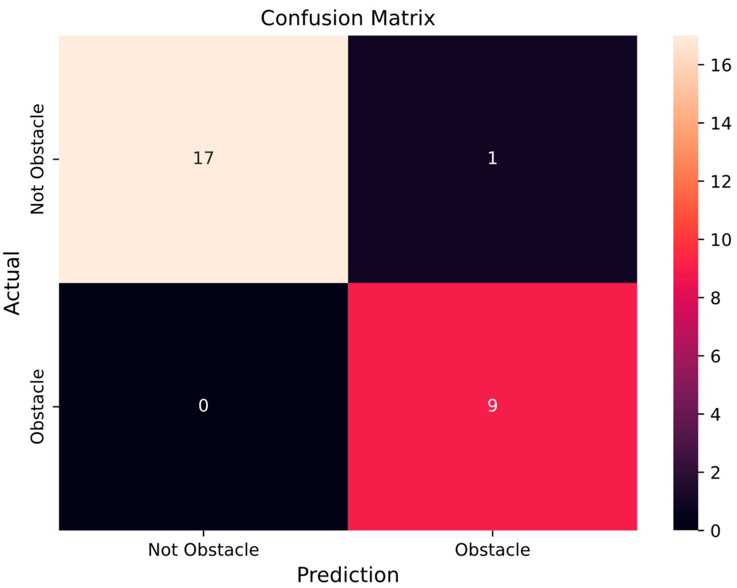
5.2. Confusion Matrix for the LBP-FFT-CNNs Classification Model
We adopt a confusion matrix to evaluate classification performance.
Figure 9 shows a confusion matrix for the proposed classification model. The horizontal line represents prediction results of the model, and the vertical line represents the actual category. The four regions represent true positive (
), false negative (
), false positive (
), and true negative (
). The
is a value between 0 and 1. When the
and
are both high, the
will also be high.
is an indicator that comprehensively considers
and
and is used to evaluate the overall performance of a binary classification model. The
of our proposed classification model reaches 0.971,
is 0.963,
is 1, and
is 0.944.
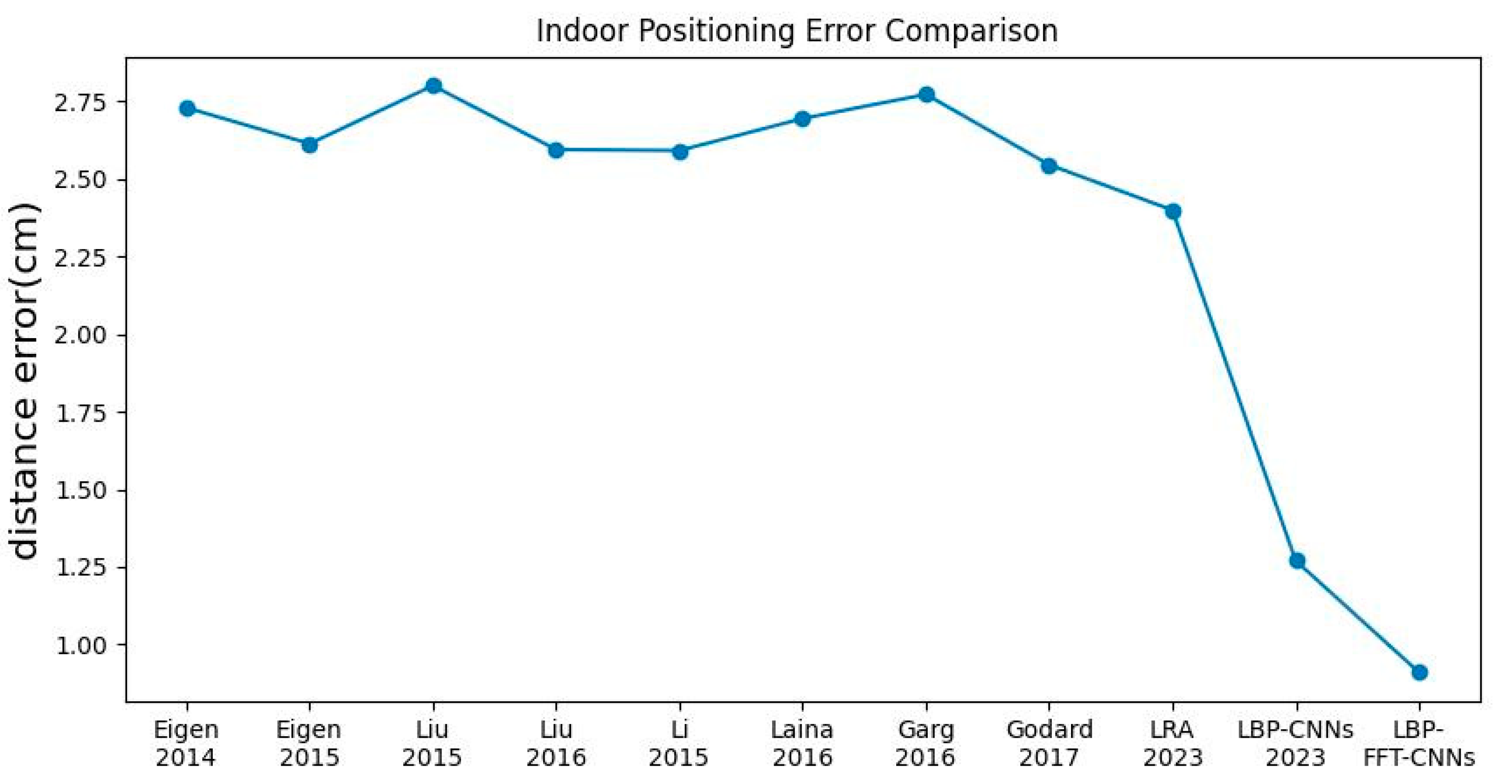
5.3. Indoor Positioning Error Comparison
We perform an indoor positioning error comparison based on the most cited depth estimation model in the past decade.
Figure 10 records their changing trends. Compared with the model proposed by Eigen et al. in 2014 [
23] and 2015 [
24], the performance of LBP-FFT-CNNs is improved by 66.7% and 65.2%, respectively. This is mainly because the multi-scale deep network model can only improve accuracy by increasing the amount of training data, but its feature extraction ability is weak. However, the LBP module in our model can better extract image features. Even if the model proposed by Liu in 2016 [
25] adds encoded super pixel information, it still has a 51.1% performance improvement compared to that proposed by Liu in 2015 [
26]. Garg et al. [
27] used stereo image pairs to achieve excellent performance, but there was still a 64.9% gap with the LBP-FFT-CNNs model. Stereoscopic image pairs may suffer from viewpoint inconsistencies because the camera’s position and orientation may not be precisely aligned or due to dynamic elements in the scene. This can lead to errors in tasks such as depth estimation. Li et al. [
28] presents a deep convolutional neural network framework combined with conditional random fields to predict scene depth or the normal surface from single monocular images. It achieved competitive results on the Make3D and NYU Depth V2 datasets. Laina [
29] inverts the parameters of Huber loss function, making it more sensitive to smaller errors but less robust to outliers. Compared with LRA method, which is also based on the MC4L device, its performance is improved by 64.2%. Godard [
30] replaced the use of explicit depth data during training with easier-to-obtain binocular stereo footage. This method saves a lot of manpower without explicit depth labels and enables real-time depth perception. However, binocular stereo lenses usually rely on texture and lighting information. Therefore, the accuracy of depth estimation may decrease for scenes that lack texture or have large lighting changes. Experimental results show that combining advanced feature extraction techniques such as LBP and FFT with CNNs can significantly improve positioning accuracy. Another important reason is the use of inertial-based indoor positioning algorithms, which greatly reduces the unstable positioning problem under complex environments with too many obstacles.
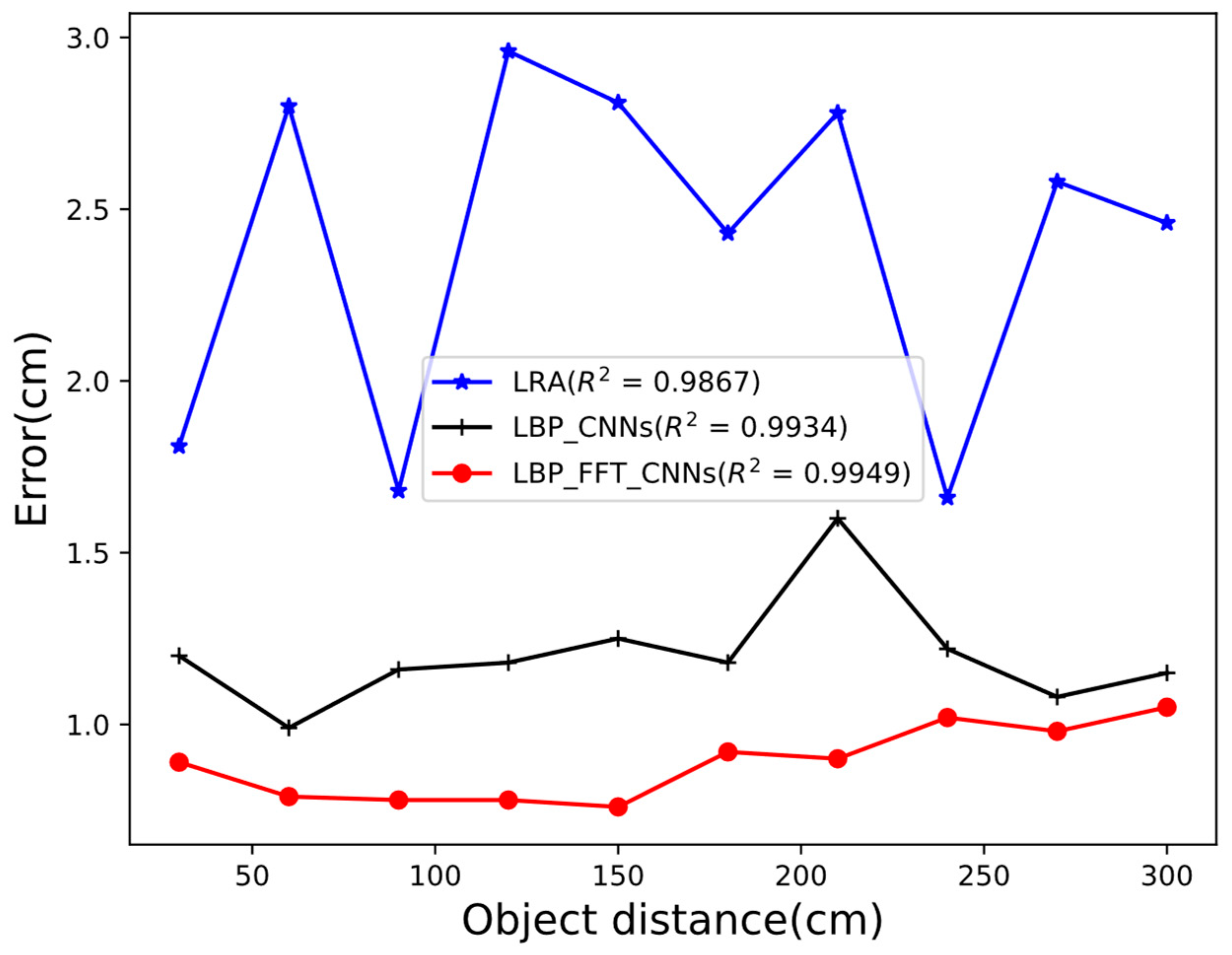
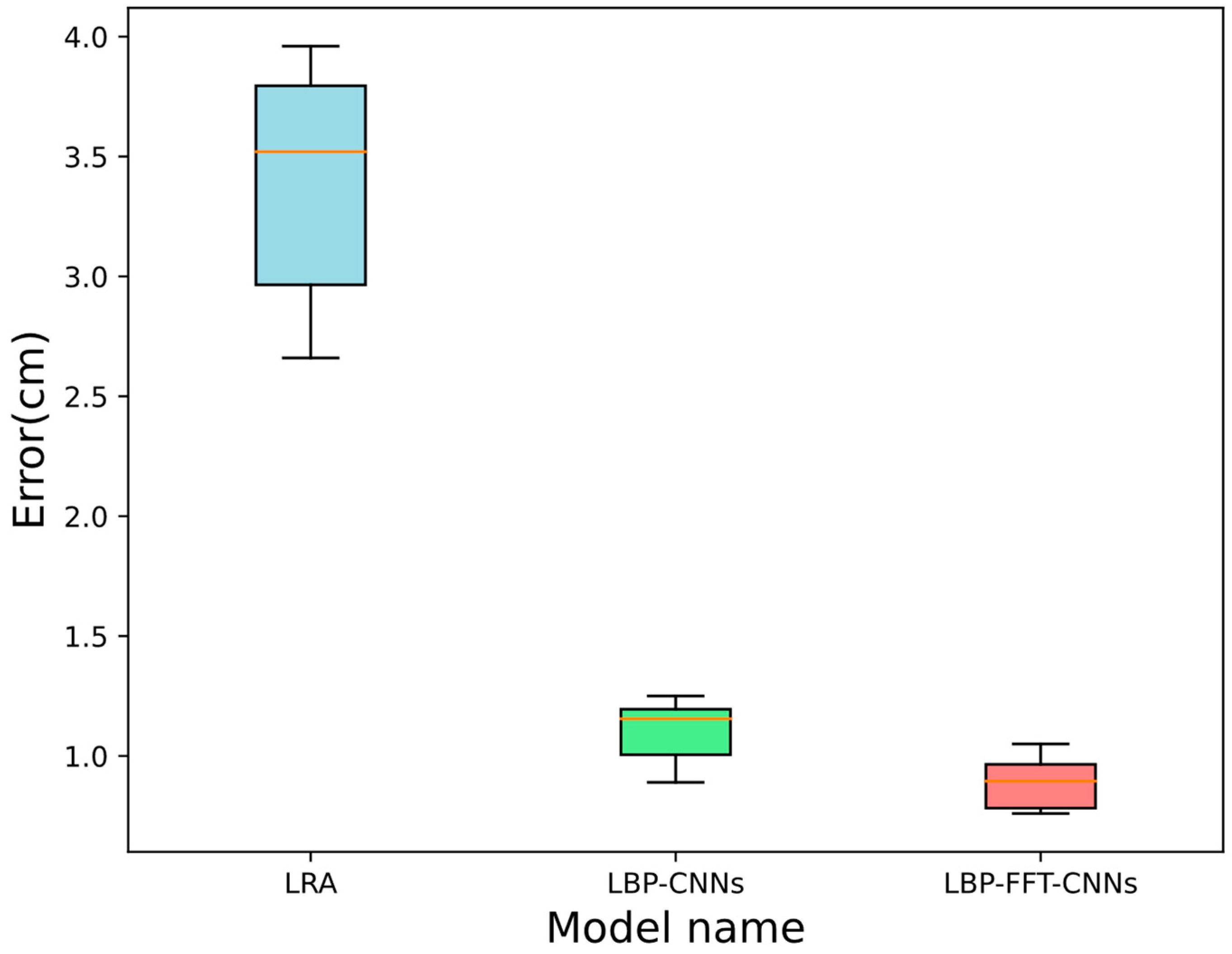
5.4. Errors from Different Locations
The LRA method is a positioning algorithm based on MC4L devices that we proposed previously. It obtains the corresponding relationship between irradiated areas and real distance using a logarithmic regression algorithm. Since lasers have different scattering effects on different target surfaces, deviations will occur in the process of positioning the laser irradiation point. Therefore, the LRA method will have an uneven distribution of measurement errors. Although LRA, LBP-CNNs, and LBP-FFT-CNNs algorithms are all based on MC4L, the LBP-CNNs method we proposed not only leads in error but also has more stable error control. Godard adopts a stereo camera to reduce errors, but it also makes errors vary greatly in different situations. The average errors of LRA, LBP-CNNs, and LBP-FFT-CNNs are 2.4 cm, 1.2 cm, and 0.9 cm. Compared with the previous two models, the LBP-FFT-CNNs model is improved by 62.5% and 24%, respectively. To evaluate the stability of model prediction and verify whether the model performs consistently at different distances, the PSI utilized is shown in Equation (34).
Figure 11 shows errors at different distances from target objects.
Here, and represent the actual distribution and expected distribution at the current location, respectively. When < 0.1, it means there is little change, and the model is basically stable. When , it means there is a slight change, which requires further observation. However, when , it indicates a significant change, indicating that the model may fail, or data may have a large drift. The PSI values of LBP-FFT-CNNs, LBP-CNNs, and LRA are 0.017, 0.019, and 0.02, respectively. Although their value is all less than 0.1, the LBP-FFT-CNNs model is more stable.
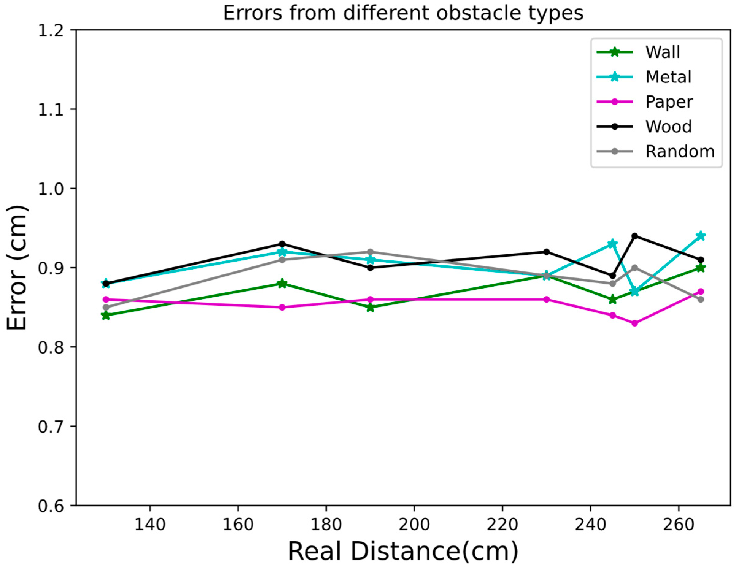
5.5. Errors from Different Environments
To evaluate model robustness in complex environments, the obstacles composed of various materials were randomly placed.
Figure 12 illustrates the positioning errors under different environmental conditions. Compared to a single material environment, the model demonstrated stable adaptability in environments with randomly placed obstacles, with a maximum error of 0.92 cm, a minimum error of 0.85 cm, and an average error of 0.89 cm. Notably, the lowest positioning error was observed when paper was used as the obstacle, with an average error of 0.8557 cm and a standard deviation of 0.0114, reflecting excellent stability. This result highlights that the low reflectivity of paper minimally impacts positioning accuracy.
In contrast, wood as an obstacle resulted in the highest average error of 0.91 cm among all conditions. This may be attributed to the wood surface’s complex texture and moderate reflectivity, which interfere with laser signals. Although error magnitude is high, the standard deviation of 0.0188 indicates moderate variability. In the absence of obstacles, the system achieved high-precision performance with an average error of 0.8757 cm, a standard deviation of 0.0188, and an error range from 0.84 cm to 0.90 cm. When metal was used as an obstacle, the average error increased slightly to 0.9043 cm, and the standard deviation of 0.0238 suggests greater error variability. This increased variability is likely due to the uneven reflective properties of metal surfaces, which affect the stability of laser detection.
To be closer to the actual usage scenario, we randomly set up obstacles in a two-meter-wide corridor and conducted the experiment in a completely dark environment.
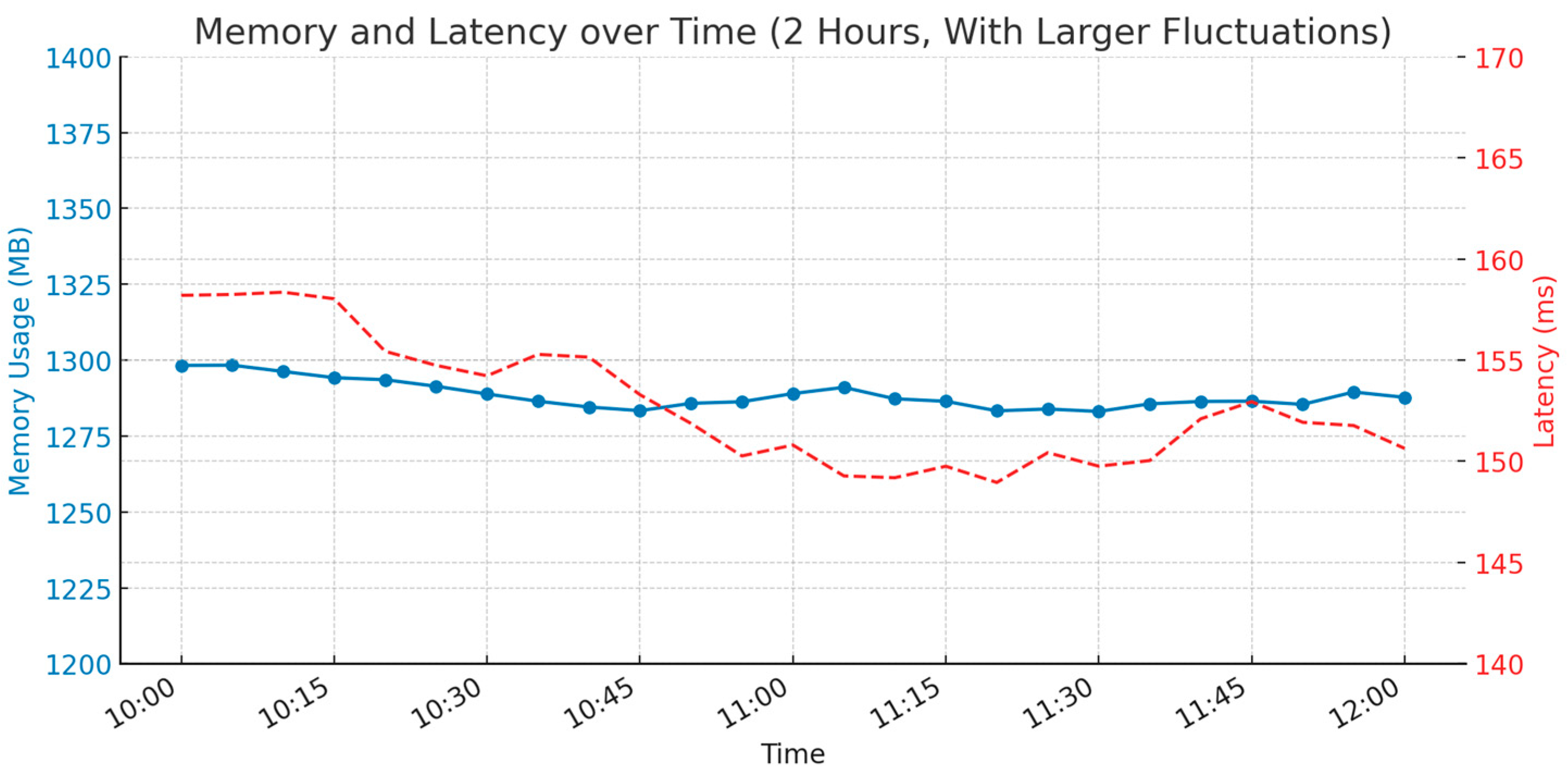
Figure 13 presents the memory usage and inference latency of the proposed LBP-FFT-CNNs model over a 2-h period, sampled every 5 min under simulated high-load and variable system conditions. Compared to baseline conditions, both metrics exhibit more pronounced fluctuations. The memory usage varies within the range of approximately 1280 MB to 1320 MB, reflecting periodic increases in background memory consumption or model memory reallocation. Despite these variations, the model maintains stability without exceeding the critical 1.4 GB threshold, ensuring continued operation within the constraints of the Raspberry Pi 4B.
Inference latency fluctuates between 145 ms and 160 ms, which corresponds to a significant increase relative to nominal performance (~45 ms). These elevated values simulate worst-case scenarios, such as concurrent sensor data processing or intermittent I/O activity. Importantly, the latency remains within acceptable bounds for applications with moderate real-time constraints.
Overall, the system demonstrates robust behavior under resource-constrained conditions, confirming the model’s viability for deployment in dynamic embedded environments.
5.6. Experimental Results Discussion
The experimental results of this study demonstrate that the LBP-FFT-CNNs method exhibits significant advantages in positioning accuracy, classification performance, and environmental adaptability. Compared to the traditional LRA method, the proposed approach reduces average error by 62.5%, while also achieving a 24% improvement over the LBP_CNNs method, indicating its superior capability in extracting image features and enhancing positioning accuracy. Furthermore, the method maintains a stable error range across different obstacle environments, with the lowest error observed in low-reflectivity materials (e.g., paper) at only 0.8557 cm, highlighting its strong environmental adaptability. Compared with the most representative depth estimation algorithms of the past decade, such as those proposed by Eigen, Liu, and Godard, the LBP-FFT-CNNs approach improves accuracy by 51.1% to 66.7%, further validating the effectiveness of integrating LBP and FFT for feature extraction. Additionally, classification experiments reveal that the proposed method achieves an F1 score of 0.971 and an accuracy of 96.3%, demonstrating not only precise target positioning but also effective obstacle classification. Overall, by incorporating multi-scale local features and frequency domain information, the LBP-FFT-CNNs algorithm enhances model robustness and exhibits superior stability in complex environments, providing a novel technological approach for high-precision indoor positioning and obstacle recognition.
6. Conclusions and Future Work
This paper presented an improved indoor positioning and obstacle recognition system for dark environments based on MC4L-IMU. To enhance recognition accuracy for objects with similar textures, we introduced FFT into the LBP-CNNs model, forming LBP-FFT-CNNs. This approach significantly improved obstacle identification accuracy. Additionally, we integrated an IMU with the MC4L device and designed an inertial-based hybrid indoor positioning algorithm. Experimental results demonstrated that the proposed LBP-FFT-CNNs model reduced the average indoor positioning error to 0.91 cm, with an obstacle recognition accuracy of 96.3%.
Compared with traditional methods, the LBP-FFT-CNNs model outperformed LRA and LBP-CNNs in positioning accuracy and stability, achieving an R2 value of 0.9949, the highest among all models. The integration of FFT effectively captured frequency domain features and leading to improved regression performance. Furthermore, the system demonstrated strong adaptability to different obstacle environments with the lowest error observed for low-reflectivity materials and stable performance under diverse conditions. Comparative analysis with state-of-the-art depth estimation methods confirmed that the LBP-FFT-CNNs model improved accuracy by 51.1% to 66.7%, underscoring its advantages in feature extraction and positioning reliability. Additionally, all models exhibited robust stability with PSI values below 0.02, ensuring consistent performance across various conditions.
Future work will explore further improvements by integrating advanced sensor fusion techniques, such as incorporating depth cameras or LiDAR [
31] to enhance obstacle recognition in more complex environments. Additionally, more sophisticated machine learning models, such as transformers or graph neural networks, will be leveraged. This could further improve recognition accuracy, particularly for objects with similar textures. Finally, large-scale field validation will be conducted to ensure broader applicability and consistent performance in real-world indoor environments.


