Article

Active Gait Retraining with Lower Limb Exoskeleton Based on Robust Force Control

by
Yukio Rosales-Luengas
,
Sergio Salazar
,
Saúl J. Rangel-Popoca
,
Yahel Cortés-García
,
Jonathan Flores
and
Rogelio Lozano
*
Department of Research and Multidisciplinary Studies, Center for Research and Advanced Studies of the National Polytechnic Institute, Mexico City 07360, Mexico
*
Author to whom correspondence should be addressed.
Appl. Sci. 2025, 15(7), 4032; https://doi.org/10.3390/app15074032
Submission received: 1 February 2025 / Revised: 4 April 2025 / Accepted: 4 April 2025 / Published: 6 April 2025

Abstract

:
This article addresses the design of a robust inner and outer loop controller for active gait retraining in individuals with leg motor weakness, using a lower limb exoskeleton with elastic joints. The proposed control algorithm for the inner loop is based on a robust force controller that considers dynamics in the sagittal plane, accounting for human and external perturbations. For the outer loop, a robust controller is proposed to ensure the tracking of the desired trajectories. Lyapunov candidate functions are used to demonstrate the stability of the closed-loop system. To validate the proposed algorithmic approach, numerical simulations and experimental tests are developed. The experimental results show excellent performance, even in the presence of external perturbations and opposing human reactions; the tracking error is minimal (MAE ≤ 0.0661 rad).

1. Introduction

People have the fundamental ability to walk to get from one place to another. However, losing this ability due to physical or psychological health problems significantly affects human lives [1]. According to the World Health Organization (WHO), spinal cord injuries, neuromuscular diseases, and muscle aging will continue to increase [2]. Traditional rehabilitation methods mainly focus on passive exercises, assisted stretching, and activities supervised by a therapist. Despite the good results obtained, traditional rehabilitation has several disadvantages, including inconsistent intensity, high physical effort required from both patients and therapists, and a lack of adaptability. As a result, research has shifted toward active rehabilitation methods using robotic devices like exoskeletons, for example, systems for assistance and gait retraining, designed to progressively improve therapy outcomes [3].
Gait rehabilitation has been revolutionized by the development of devices such as exoskeletons and advanced rehabilitation systems. These innovations have transformed traditional rehabilitation techniques, making them more comprehensive and effective. This new approach incorporates the use of exoskeletons, enabling patients to actively participate in their rehabilitation process [4].
Commercial exoskeletons like the EXO-H3 [5], Atalante, Ekso [6], and Hank have achieved important advances in gait rehabilitation and have also demonstrated their potential by integrating advanced control algorithms that allow for customized trajectories and speeds based on patient needs. Pattern recognition techniques further enhance the adaptation of the exoskeleton to the patient [7,8,9,10], making rehabilitation more effective for conditions such as hemiplegia and quadriplegia.
Understanding movement intention is crucial for making accurate trajectory predictions. This challenge has been effectively addressed using robust control mechanisms. For example, reference [11] discusses the implementation of adaptive sliding mode variable admittance control. Meanwhile, references [12,13] explore the use of adaptive backstepping sliding mode techniques and hybrid approaches integrating neural networks.
Two strategies have shown particular promise in enhancing control stability and adaptability in gait exoskeletons. The first strategy proposes using sliding mode-based observers and neural networks to estimate unmeasured variables, such as joint velocities, and employing iterative learning control (ILC) to progressively adjust trajectories based on previous repetitions.
The approach proposed in [14] demonstrates that accurate trajectory tracking can be achieved without velocity measurements using only a neural network-based observer and sliding mode control to estimate and compensate for uncertainties in the system. Applying this strategy to exoskeletons for rehabilitation and gait retraining would reduce the dependence on additional sensors, thereby improving the robustness of the control to external perturbations and variations in patient characteristics.
Another strategy is to use iterative learning control, such as that presented in [15], which offers a way to optimize the adaptation of the exoskeleton to the patient. By repeating movements, the system can adjust its control parameters with the objectives of compensating for repetitive perturbations and improving trajectory tracking accuracy. This progressive learning capability is particularly beneficial for rehabilitation with this type of exoskeleton.
Using and implementing the control strategies described above in an exoskeleton allows for a more efficient and adaptable system capable of predicting and correcting trajectories without the need for direct speed measurements while simultaneously improving its performance with everyday use. Such control strategies can open new possibilities and opportunities for the personalization of rehabilitation by automatically adjusting gait patterns based on user progress without manual intervention from the therapist.
Additionally, ref. [15] provides a methodology to properly tune the adaptive behavior of rehabilitation exoskeletons to better suit patients. By repeating the sequence of motion, it adapts its control parameters to eliminate regular disturbance and enhance the tracking accuracy of the trajectory. Such progressive capabilities in learning are most welcome in scenarios of therapy because the performance of patients keeps changing.
Another approach to detecting movement intention involves using electromyographic signals [16] to adjust the torque sent to the motors in real time, enabling safe and progressive training. Additionally, human-in-the-loop control [17,18] has been utilized for combined data acquisition while the patient is wearing the exoskeleton. This approach achieves balance optimization through the zero moment point methodology, which allows patients to walk without crutches or other support devices, resulting in better stability and increased patient confidence.
For human conditions like hemiplegia, exoskeletons have been combined with motion capture systems to provide an analysis of symmetry between both the functional and the affected leg [19,20]. This system facilitates the design and analysis of motion trajectories from the patient’s functional limb and allows for replication in the damaged limb, aiming to aid in the recovery of symmetrical walking patterns. In [21], neuromuscular rehabilitation was conducted using a system called Progressive Assist-as-Needed Control, which employs muscular signals to adjust the support. This system allows for a smooth transition between different levels of assistance and adapts to the patient’s progress.
Reinforcement Learning (RL), Deep Learning (DL), and Deep Reinforcement Learning (DRL) [22,23,24,25] have been explored as alternative approaches, as these techniques offer promising results due to their robustness against disturbances and their ability to adapt to varying conditions. For instance, in [24], researchers developed a DRL-based controller for lower limb rehabilitation that employs a neural controller that adapts to several forces applied by the human, without requiring parameter adjustments. This methodology has demonstrated efficiency in reducing tracking error, suggesting that DRL models offer adaptable assistance. Furthermore, in [25], an exoskeleton was developed using DL for post-neurovascular rehabilitation. This system uses convolutional neural networks and recurrent networks to interpret electromyography signals, aiming to adapt the motor actuator function according to the patient’s condition. Its application allows for better precision in exoskeleton control, achieving adaptation in individual gait parameters and reducing external disturbances. Given these advances, the use of DL and DRL represents a viable alternative for the control of rehabilitation exoskeletons, optimizing patient rehabilitation. These strategies facilitate the elimination of tracking errors and reductions in disturbances during gait, enabling the development of efficient and customized rehabilitation technologies.
Additionally, exoskeletons have been designed with anthropometric considerations that allow them to adjust to gait parameters [26], effectively eliminating tracking errors and disturbances [27]. Innovative devices with 12 degrees of freedom [28] have also been created. These devices can operate effectively against unmodeled uncertainties, potentially enhancing the autonomy and flexibility of the exoskeleton and the patient, thereby opening a wide range of opportunities for gait rehabilitation.
Recent advancements propose the integration of neural networks, including recurrent neural networks such as Long Short-Term Memory (LSTM) architectures [29,30,31,32], as well as optimization algorithms like fuzzy logic controllers [33,34]. These innovations enhance adaptability and enable real-time adjustments based on biomechanical data obtained from IMU sensors.
Controllers based on LSTM networks and fuzzy logic offer significant benefits in gait rehabilitation. On one hand, fuzzy logic controllers stand out for their ability to handle system uncertainties and adapt to various gait velocities. On the other hand LSTM networks are notable for their capacity to accurately predict movement patterns and trajectories by capturing temporal dependencies in the data. However, despite these advantages, these controllers still face challenges. For instance, they may struggle when applied to patients who differ significantly from the analyzed population or when the data collection conditions vary.
Furthermore, multimodal exoskeletons have been developed that combine active and passive rehabilitation [35], achieving greater interactivity between the patient and the gait rehabilitation device. The use of these exoskeletons has demonstrated positive results in improving muscular coordination and enabling faster and more interactive rehabilitation for the patient [36]. However, these improvements are not yet conclusive and require more comprehensive studies on the benefits of those exoskeletons. Nevertheless, it is expected that such rehabilitation technologies will continue to improve, with the main objective of complementing traditional rehabilitation in a more comfortable, adaptive, and inclusive manner.
The main contribution of this article is the development of a robust inner–outer loop controller for a lower limb exoskeleton designed to assist in active gait retraining. A robust sliding mode controller is proposed to enable robust and asymptotic convergence of the exoskeleton’s angular trajectories. To prevent chattering effects from affecting the exoskeleton user and causing wear on the exoskeleton itself, two solutions are proposed: first, elastic serial actuators are used, and the control algorithm is modified to reduce or even eliminates chattering effects. In this way, a robust torque controller is designed to act in a cascade with the first controller, also based on sliding modes, to ensure robust and asymptotic torque convergence.
This paper is organized as follows. A description of the exoskeleton and its dynamic model are presented in Section 2. Section 3 presents the design of the robust force control, while the design of the robust tracking control is presented in Section 4 and the results of the numerical simulation and experimental implementation are reported in Section 5. Finally, the conclusions are presented in Section 6.

2. Materials and Methods

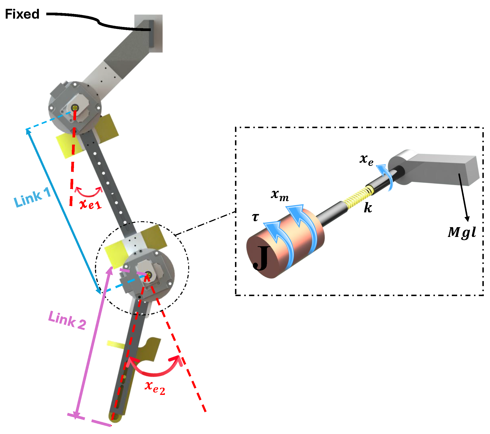
2.1. Exoskeleton Description

In order to perform the rehabilitation exercises, this work used the anthropomorphic lower limb exoskeleton shown in Figure 1a, which has two robotic legs with two links and two elastic joints each. The anthropometric design of the exoskeleton allows for easy adjustment to the patient’s legs, ensuring that the patient’s movements are appropriately adapted to the exoskeleton’s legs (Figure 1b). The elastic element in the exoskeleton’s flexible joints acts as a shock absorber, reducing the actuator inertia felt by the user and thereby increasing safety and comfort. The flexible coupling between the user and the motor protects the user’s joints from impact loads and other undesirable interactions. Additionally, it allows for small patient movements, further enhancing comfort.
In addition to the robotic legs, the exoskeleton has an additional loading system so that the legs of the exoskeleton do not support the patient’s weight during rehabilitation routines but the loading system does this task, leaving the exoskeleton legs only to move the patient’s legs to complete the rehabilitation routine. The exoskeleton lifting system consists of a double four-bar mechanism operated by two linear actuators (model LACT6P), each capable of withstanding a load of 50 kg. The system is anchored at one end to the hand supports of a standard treadmill and at the other end to the mechanical legs, allowing them to move up and down while maintaining vertical alignment. The patient is supported by a harness attached to the upper bar of the harness frame, which is connected to the four-bar system at the same point as the mechanical legs.
To generate movement in each leg, the exoskeleton is equipped with FHA-14C-100 electric actuators at the hip and knee joints, capable of delivering up to 28 Nm of torque. Each actuator is coupled to a torsional spring with a stiffness of 138.65 Nm/rad, through which mechanical power is transmitted to the links of each leg. The angular displacement at each joint is measured directly by two AMT203-V absolute rotary encoders from CUI devices. Two encoders per joint are used to simultaneously measure the angular position of the motor (before the spring) and the angular position of the link (after the spring) at the same joint. Angular velocity is obtained via software by numerically differentiating the angular position.
Data acquisition and processing, as well as the generation of control statements, are carried out on a myRIO card from National Instruments.

2.2. Exoskeleton Dynamic Model

Figure 2 shows a simple diagram of one leg of the exoskeleton with the elastic joints shown in Figure 1a. The model in this section is the same for both legs.
The dynamic model of the exoskeleton with elastic joints is derived from the Euler–Lagrange approach and is expressed as follows:
M e ( x e ) x ¨ e + C e ( x e , x ˙ e ) x ˙ e + g e ( x e ) K x m x e = 0
J m x ¨ m + B x ˙ m + K x m x e = τ m
where the angular positions of links 1 (hip) and 2 (knee) of the exoskeleton are denoted by the vector expressed as x e = [ x e 1 x e 2 ] T , while the angular positions of motors 1 (hip) and 2 (knee) are denoted by the vector expressed as x m = [ x m 1 x m 2 ] T . The exoskeleton inertia matrix is given by M e R 2 × 2 , the exoskeleton Coriolis matrix is given by C e R 2 × 2 , the gravitational forces vector is given by g e R 2 , and K is a diagonal matrix formed by the torsional spring stiffness coefficients with the following form: K = d i a g { k 1 , k 2 } . J = d i a g { J 1 r 1 , 1 2 , J 2 r 1 , 2 2 } is a diagonal matrix formed by the product of the inertia moment of the rotors and the square of the gear ratio. The viscous friction values of the motors form the diagonal matrix (B). Finally, the torques of the actuators of the hip and knee form the input vector expressed as τ m R 2 .
Matrices M e , C e , and g e are made up of the following elements:
M e 11 ( x e ) = I 1 + I 2 + l 1 2 m 2 + l c 1 2 m 1 + l c 2 2 m 2 + 2 l 1 l c 2 m 2 c o s ( x e 2 ) M e 12 ( x e ) = I 2 + l c 2 2 m 2 + l c 2 2 m 2 + l 1 l c 2 m 2 c o s ( x e 2 ) M e 21 ( x e ) = I 2 + l c 2 2 m 2 + l c 2 2 m 2 + l 1 l c 2 m 2 c o s ( x e 2 ) M e 22 ( x e ) = I 2 + m 2 l c 2 2
C e 11 ( x e , x ˙ e ) = m 2 l 1 l c 2 s i n ( x e 2 ) x ˙ e 2 C e 12 ( x e , x ˙ e ) = m 2 l 1 l c 2 s i n ( x e 2 ) [ x ˙ 1 + x ˙ e 2 ] C e 21 ( x e , x ˙ e ) = m 2 l 1 l c 2 s i n ( x e 2 ) x ˙ 1 C e 22 ( x e , x ˙ e ) = 0
g e 1 ( x e ) = [ m 1 l c 1 + m 2 l 1 ] g s i n ( x e 1 ) + m 2 g l c 2 s i n ( x e 1 + x e 2 ) g e 2 ( x e ) = m 2 g l c 2 s i n ( x e 1 + x e 2 )
where I 1 and I 2 are the inertia values of links 1 and 2, respectively; l 1 and l 2 are the lengths of links 1 and 2, respectively; l c 1 and l c 2 are the lengths at the center of mass of links 1 and 2, respectively; and m 1 and m 2 are the masses of links 1 and 2, respectively. g represents acceleration due to gravity.

3. Force Control of an Exoskeleton with Elastic Joints

The dynamic model of the exoskeleton with elastic joints is defined by Equations (1a) and (1b), while the dynamic model of a human leg can be defined by the following form:
M h ( x h ) x ¨ h + C h ( x h , x ˙ h ) x ˙ h + g h ( x h ) = τ h
Let us define the spring torque ( τ s ) as
τ s = K x m x e
Assumption 1.
The exoskeleton is attached to the lower limb, so the position of the person is the same as that of the exoskeleton, that is, x h = x e .
With these assumptions, we have the following dynamic model of the exoskeleton plus the human leg:
M e + M h ( x e ) x ¨ e + C e + C h ( x e , x ˙ e ) x ˙ e + g e + g h ( x e ) = τ h + τ s J m x ¨ m + B x ˙ m = τ m τ s
Rewriting the previous equation considering M = M e + M h , C = C e + C h , and g = g e + g h , where the dynamic model of a human is not known exactly, let us define Φ ( x e , x ˙ e ) , including all the parametric uncertainties, obtaining Equation (8a)
M ( x e ) x ¨ e + C ( x e , x ˙ e ) x ˙ e + g ( x e ) + Φ ( x e , x ˙ e ) = τ h + τ s
J m x ¨ m + B x ˙ m = τ m τ s
Taking the second derivative of (6) and solving for x ¨ m yields
τ ¨ s = K x ¨ m x ¨ e
x ¨ m = K 1 τ ¨ s + x ¨ e
Solving for x ¨ e from (8a) and substituting it into (10) yields
x ¨ m = K 1 τ ¨ s + M 1 τ h + M 1 τ s M 1 C x ˙ e M 1 g M 1 Φ
Substituting (11) into (8b) and solving for τ m yields
K 1 J m τ ¨ s + M 1 J m τ h + M 1 J m τ s M 1 J m C x ˙ e M 1 J m g M 1 J m Φ + B x ˙ m = τ m τ s
K 1 J m τ ¨ s + I + M 1 J m τ s M 1 J m C x ˙ e M 1 J m g + M 1 J m τ h M 1 J m Φ + B x ˙ m = τ m
Equation (13) can be rewritten as follows:
a 2 τ ¨ s + a 1 τ ˙ s + a 0 τ s = τ m + b C x ˙ e + g + Γ 1 ( t )
where b = M 1 J m , a 2 = K 1 J m > 0 , a 1 = 0 , a 0 = I + b > 0 , and Γ 1 ( t ) = Φ τ h + b 1 B x ˙ m , considering that Γ 1 ( t ) is bounded as Γ 1 < Γ 1 m a x .

Stability Proof

Consider the following control law [37,38]:
τ m = a 2 τ ¨ d 2 λ τ ˜ ˙ λ 2 τ ˜ + a 1 τ ˙ s + a 0 τ s ρ 1 s 1 s i g n s 1 b C x e + g
where we define the torque error as τ ˜ = τ s τ d and consider that ρ 1 > b Γ 1 m a x .
The sliding surface in (15) is defined as
s 1 = τ ˜ ˙ + λ τ ˜
where λ > 0 .
With the intention of proving that the system is stable, we propose the following Lyapunov candidate function:
V 1 ( t ) = 1 2 s 1 T a 2 s 1
With this form, V 1 is positive definite. The equation that describes the closed-loop system is derived by substituting the control law (15) into (14) as
a 2 τ ¨ s + a 1 τ ˙ s + a 0 τ s = a 2 τ ¨ d 2 λ τ ˜ ˙ λ 2 τ ˜ + a 1 τ ˙ s + a 0 τ s b ( C x e + g ) ρ 1 s 1 s i g n ( s 1 ) + r ( C x e + g + Γ 1 ( t ) )
Rewriting the previous equation, the following is obtained:
a 2 ( τ ¨ s τ ¨ d + 2 λ τ ˜ ˙ λ 2 τ ˜ ) = b Γ 1 ρ 1 s 1 s i g n ( s 1 )
Considering that τ ˜ ¨ = τ ¨ s τ ¨ d ,
a 2 ( τ ˜ ¨ + λ τ ˜ ˙ + λ ( τ ˜ ˙ λ τ ˜ ) ) = b Γ 1 ρ 1 s 1 s i g n ( s 1 )
Using s ˙ 1 = τ ˜ ¨ + λ τ ˜ ˙ and s 1 = τ ˜ ˙ + λ τ ˜ yields
a 2 ( s ˙ 1 + λ s 1 ) = b Γ 1 ρ 1 s 1 s i g n ( s 1 )
Then, the time derivative of the Lyapunov function (V) is calculated as
V ˙ 1 = s 1 T a 2 s ˙ 1 = s 1 T a 2 a 2 1 b Γ 1 a 2 1 ρ 1 s 1 s i g n ( s 1 ) λ s 1
Then, we obtain
V ˙ 1 = s 1 T a 2 λ s 1 + s 1 b Γ 1 ρ 1 s 1 3 2 < 0 s 1 R 2 { 0 }
Next, for s 1 = 0 and V ˙ 1 = 0 , it follows that τ ˜ ˙ + λ τ ˜ = 0 , then τ ˜ ˙ 0 and τ ˜ 0 , i.e., τ s τ d asymptotically.

4. Tracking Control of the Exoskeleton

Based on the result obtained above, we can rewrite (8a) as
M ( x e ) x ¨ e + C ( x e , x ˙ e ) x ˙ e + g ( x e ) Γ 2 ( t ) = τ s = τ d
where Γ 2 ( t ) = τ h Φ ( x e , x ˙ e ) , considering that Γ 2 ( t ) is bounded as Γ 2 < Γ 2 m a x .
Let us consider the following control law for (24):
τ d = M x ¨ d 2 γ x ˜ ˙ γ 2 x ˜ + C x ˙ + g ρ 2 s 2 s i g n s 2
where we define the position error as x ˜ = x e x d consider that ρ 2 > Γ 2 m a x .
The sliding surface in (25) is defined as
s 2 = x ˜ ˙ + γ x ˜
where γ > 0 .
The closed-loop equation is obtained by replacing the control action ( τ d ) of the control law (25) in Equation (24)
M x ¨ e = M x ¨ d 2 γ x ˜ ˙ γ 2 x ˜ + C x ˙ e + g ρ 2 s 2 s i g n s 2 C x ˙ e g + Γ 2
Then, Equation (27) is reduced to
M s ˙ 2 + γ s 2 = Γ 2 ρ 2 s 2 s i g n s 2

Stability Proof

In order to provide the stability system for (28), the following Lyapunov candidate function is proposed:
V 2 ( t ) = 1 2 s 2 T M s 2
The derivative with respect to time is
V ˙ 2 = s 2 T M s ˙ 2 = s 2 T M M 1 Γ 2 M 1 ρ 2 s 2 s i g n ( s 2 ) γ s 2
Then, we obtain
V ˙ 2 = s 2 T M γ s 2 + s 2 Γ 2 ρ 2 s 2 3 2 < 0 s 2 R 2 { 0 }
Next, similar to the result of Equation (23), for s 2 = 0 , V ˙ 2 = 0 , it follows that x ˜ ˙ + γ x ˜ = 0 , then x ˜ ˙ 0 and x ˜ 0 , i.e., x e x d asymptotically. In summary, using the first sliding surface ( s 1 ) and the proposed Lyapunov function ( V 1 ), we achieve exponential convergence of τ s to τ d . Similarly, for the error ( x ˜ ), the sliding surface ( s 2 ) and the Lyapunov function ( V 2 ) ensure that the error converges to zero.

5. Experimental and Simulation Results

Figure 3 shows the total structure of the proposed control system, which consists of an internal control loop where the robust force control stabilizes the force applied to each link according to a desired torque and an external loop, where the tracking control stabilizes the path of the links in a desired trajectory.
The desired trajectories for the gait cycle are given by [39]
x d 1 = 17.2 s i n ( 0.08 ω t + 0.24 ) + 69.61 s i n ( 1.00 ω t + 1.72 ) + 6.90 s i n ( 0.17 ω t + 2 ) + 4 s i n ( 2 ω t 1.72 ) + 1.68 s i n ( 2.99 ω t 0.01 ) + 1.63 s i n ( 0.36 ω t + 2.31 ) + 0.70 s i n ( 0.44 ω t + 4.24 ) + 48.17 s i n ( 1.01 ω t + 4.81 ) , x d 2 = 44.7 s i n ( 0.08 ω t + 0.36 ) + 21.13 s i n ( 0.99 ω t 2.92 ) + 16.07 s i n ( 2 ω t 0.94 ) + 20.08 s i n ( 0.15 ω t + 2.44 ) + 4.37 s i n ( 2.99 ω t 0.02 ) + 20.92 s i n ( 0.34 ω t + 2.98 ) + 18.45 s i n ( 0.35 ω t + 6 ) + 1.27 s i n ( 3.98 ω t 0.65 ) ,
where x d 1 is the desired trajectory of the hip, x d 2 is the desired trajectory of the knee, and ω is the frequency of the walking cycle.
The trajectories for the right and left legs are the same but offset from each other by a half cycle. The results shown below (both simulation and experimental) are only from the right leg.

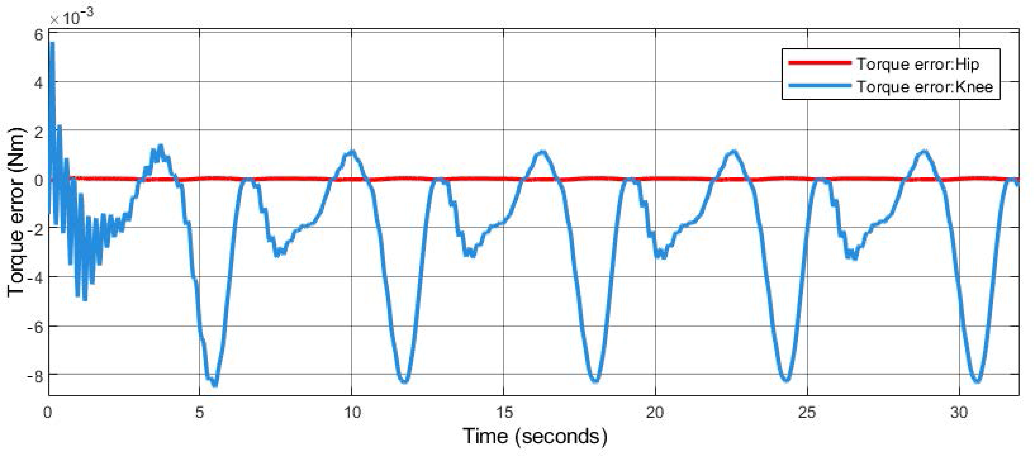
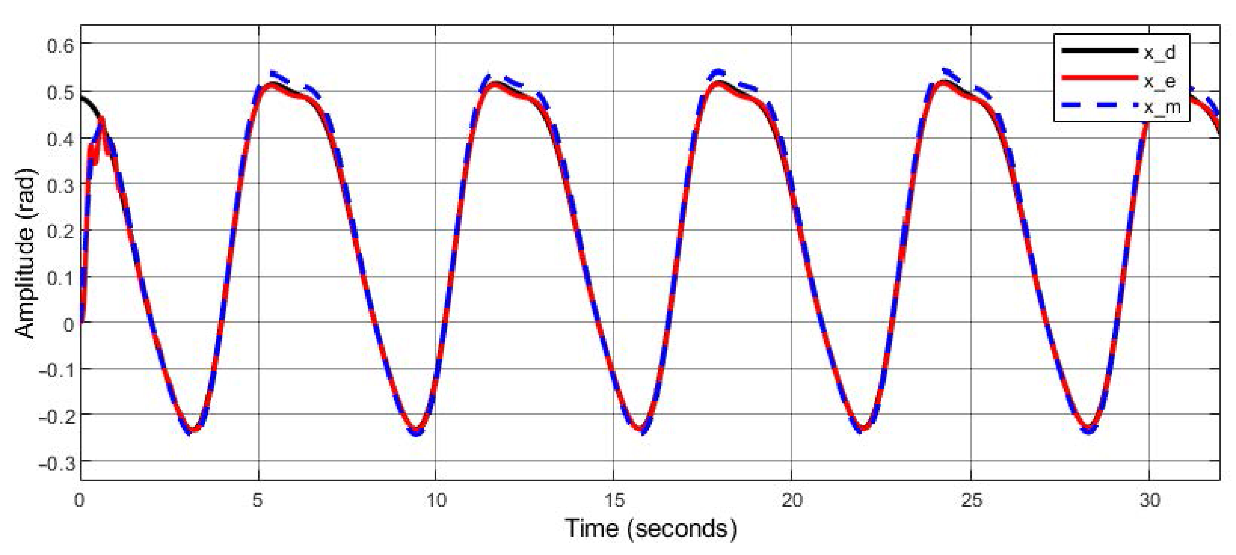
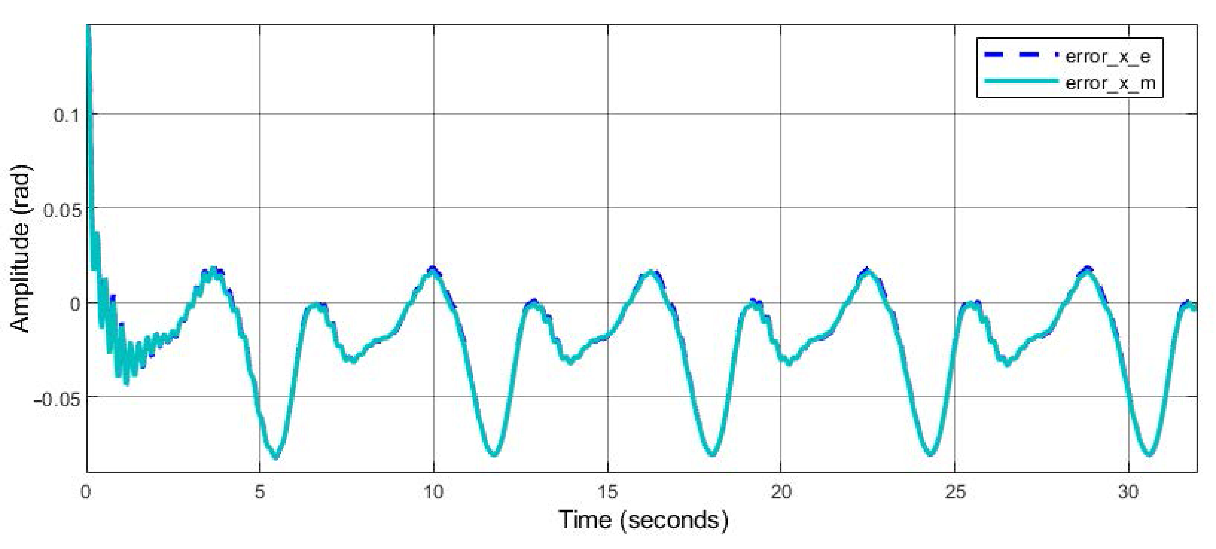
5.1. Simulation Results

For the simulation stage, the Simulink environment was used, which is a tool included in MATLAB R2023b (The MathWorks, Inc., Natick, MA, USA) for modeling, simulation, and analysis of dynamic systems through block diagrams. In the Simulink environment, a Runge–Kutta solver was used with a fixed step size of 0.0005 s and a total simulation time of 32 s. The parameters of the exoskeleton used for the simulation are shown in Table 1.
The control parameters for the force controller and tracking controller are shown in Table 2.
For the simulation tests, five walking cycles were performed for the hip and knee, and sine signals were added as external disturbances, which represent the (more or less weak and intermittent) efforts that the patient consciously makes to execute the walk process for himself.
The first stage to be checked is in the internal control loop, where the force control stabilizes the torque generated by the spring. Figure 4 displays the spring torque ( τ s ), tracking the desired torque ( τ d ) for both the hip and knee. In this figure, the desired torque for the hip (Tau_d:Hip on the graph) is represented by the black line, the desired torque for the knee (Tau_d:Knee on the graph) is represented by the blue line, the torque of the hip spring (Tau_s:Hip on the graph) is represented by the dotted yellow line, and the torque of the knee spring (Tau_s:Knee on the graph) is represented by the pink dotted line.
Figure 5 shows minimal torque errors in this interval ( | τ ˜ s 1 | < 0.009 Nm, | τ ˜ s 2 | < 0.001 Nm).
Figure 6 shows the output torque ( τ m ) of the force control for both the hip and knee. It is observed that at the beginning of the graph, there are decreasing oscillations, followed by gentle behavior; this happens because in the simulation far initial conditions were proposed in the desired trajectory and in the exoskeleton. This is not the case in experimental tests, since the walking exercise always starts with zero initial conditions for both the exoskeleton and the desired trajectory; from that point on, the steps begin smoothly. However, for the simulation, it was decided to leave far initial conditions to observe the extreme of the system response.
Figure 7 shows the tracking of the hip joint for the five running cycles performed in the simulation; the black line represents the desired trajectory ( x d ; x_d in the graph), the red line represents the trajectory running the exoskeleton ( x e ; x_e in the graph), and the blue dotted line represents the trajectory of the actuator ( x m ; x_m in the graph). This figure depicts the response to step entry generated by the difference in initial conditions between the desired trajectory and the exoskeleton. The exoskeleton trajectory reaches the desired trajectory in less than 1 s with an over-damped response, from which point the exoskeleton trajectory follows the desired trajectory.
Figure 8 shows the followed trajectory but now from the knee joint for the five running cycles executed in the simulation; as in Figure 7, the black line represents the desired trajectory ( x d ; x_d in the graph), the red line represents the trajectory running the exoskeleton ( x e ; x_e in the graph), and the blue dotted line represents the trajectory of the actuator ( x m ; x_m in the graph). It can be observed that, similar to the figure above, the trajectory of the exoskeleton follows the desired trajectory.
The hip tracking error is shown in Figure 9, where the blue dotted line represents the exoskeleton tracking error (error_x_e in Figure 9), while the motor tracking error (error_x_m in Figure 9) is represented by the cyan line. It can be observed that once the exoskeleton reaches the reference, the error is less than 0.2 rad.
Finally, the knee tracking error is shown in Figure 10, where, as in Figure 9, the dotted blue line represents the exoskeleton tracking error (error_x_e in Figure 10), while the engine tracking error (error_x_m in the figure) is represented by the cyan line. The tracking error for the knee is less than 0.12 rad.

5.2. Experimental Results

The rehabilitation exoskeleton was tested on a healthy subject of 31 years with a weight of 50 kg and a height of 1.6 m.
The experiment consists of the following steps: First, the exoskeleton is fitted to the subject. Second, the exoskeleton is turned on, and the speed and amplitude of the steps are adjusted to a slow walk, which is consistent with the rehabilitation exercises, while the subject is asked to try to walk gently, simulating muscle weakness.
The result of the internal control loop is shown in Figure 11, where the desired torque for the hip (Tau_d:Hip on the graph) is represented by the black line, the torque of the hip spring (Tau_s:Hip on the graph) is represented by the dotted magenta line, the desired torque for the knee (Tau_d:Knee on the graph) is represented by the blue line, and the torque of the knee spring (Tau_s:Knee on the graph) is depicted by the red dotted line. In this figure, it can be observed that torque tracking is almost perfect for the hip, while it presents some differences for the knee.
Figure 12 shows the output torque ( τ m ) of the force control for both the hip and knee. This figure shows that the output signal is chatter-free because the control law was obtained by the use of modified sliding modes.
Figure 13 shows the trajectory tracking of the hip joint for the five running cycles; the black line represents the desired trajectory ( x d ; x_d in the graph), the red line represents the trajectory running the exoskeleton ( x e ; x_e in the graph), and the blue dotted line represents the trajectory of the actuator ( x m ; x_m in the graph). It can be observed that the exoskeleton trajectory follows the desired trajectory.
Figure 14 shows the trajectory tracking from the knee joint; as in Figure 7, the black line represents the desired trajectory ( x d ; x_d in the graph), the red line represents the trajectory running the exoskeleton ( x e ; x_e in the graph), and the blue dotted line represents the trajectory of the actuator ( x m ; x_m in the graph). The exoskeleton follows the desired trajectory.
Table 3 shows the Mean Squared Error (MSE) and Mean Absolute Error (MAE) observed in the tracking of the desired trajectories for both the hip and knee.

6. Conclusions

An exoskeleton for active gait retraining is presented, featuring elastic joints. The mathematical model, which accounts for human dynamic interaction and the elastic response of motor actuators, was derived using the Euler–Lagrange approach. Force control algorithms were implemented to accurately track the desired trajectories. These control strategies demonstrated robustness against human reactions and external disturbances by utilizing sliding mode controllers. Implementing the proposed controller required knowledge of the full state, including both position and velocity variables. In this case, velocity estimation was used. An alternative approach involves using velocity sensors to directly acquire this variable.
Due to the elastic constant in the joints, the input control exhibited some oscillations. However, the leg trajectories (hip and knee) maintained smooth performance, depending on the elastic constant (K), which was the intended objective of the elastic joints. Experimental results demonstrated good performance even under external perturbations and opposing human reactions, with minimal tracking errors (MSE ≤ 0.0065 rad2 and MAE ≤ 0.0661 rad). Some typical delays were observed due to the spring constant. Adjusting the elastic constant (K) could reduce this lag and increase joint stiffness between the human and the exoskeleton. Ideally, a soft spring is preferable, but it introduces oscillations in the link.
Experimental tests were conducted on a healthy subject. In this case, human reactions were more pronounced than those expected from a non-healthy individual. Despite this, the control strategies effectively absorbed the perturbations caused by these reactions.

Author Contributions

Conceptualization, Y.R.-L., S.J.R.-P. and Y.C.-G.; Methodology, Y.R.-L.; Software, Y.R.-L.; Validation, Y.R.-L., S.J.R.-P. and Y.C.-G.; Formal analysis, Y.R.-L., S.S. and J.F.; Investigation, Y.R.-L., S.J.R.-P., Y.C.-G. and J.F.; Resources, R.L.; Data curation, Y.R.-L.; Writing—original draft, Y.R.-L., S.J.R.-P. and Y.C.-G.; Writing—review and editing, Y.R.-L., S.S. and R.L.; Visualization, Y.R.-L. and S.S.; Supervision, Y.R.-L. and R.L.; Project administration, S.S. and R.L.; Funding acquisition, S.S. and R.L. All authors have read and agreed to the published version of the manuscript.

Funding

This research received no external funding.

Institutional Review Board Statement

Not applicable.

Informed Consent Statement

Not applicable.

Data Availability Statement

Data are contained within the article.

Conflicts of Interest

The authors declare no conflicts of interest.

References

  1. Instituto de Salud para el Bienestar. Día Mundial de la Rehabilitación Motriz—23 de Marzo. Available online: https://www.gob.mx/insabi/articulos/dia-mundial-de-la-rehabilitacion-motriz-23-de-marzo (accessed on 31 January 2025).
  2. OMS and Banco Mundial. Informe Mundial sobre la Discapacidad 2011; Organización Mundial de la Salud & Banco Mundial: Geneva, Switzerland, 2011. [Google Scholar]
  3. Wang, Y.; Tian, Y.; Guo, Y.; Wang, H. Active torque-based gait adjustment multi-level control strategy for lower limb patient–exoskeleton coupling system in rehabilitation training. Math. Comput. Simul. 2024, 215, 357–381. [Google Scholar] [CrossRef]
  4. Gorgey, A.S. Robotic exoskeletons: The current pros and cons. World J. Orthop. 2018, 9, 112. [Google Scholar] [PubMed]
  5. Ramos, J.; Espuela, E.M.; Lora Millán, J.S.; Castano, J.A.; Borromeo, S.; Nieto, R.; Fernández, P.; Carballeira, J.; del Ama, A.J. Estrategia de control de un robot de rehabilitación de la marcha pseudoestacionario. J. Autom. 2023, 44, 95–98. [Google Scholar] [CrossRef]
  6. Zhu, F.; Kern, M.; Fowkes, E.; Afzal, T.; Contreras-Vidal, J.L.; Francisco, G.E.; Chang, S.H. Effects of an exoskeleton-assisted gait training on post-stroke lower-limb muscle coordination. J. Neural Eng. 2021, 18, 046039. [Google Scholar] [CrossRef]
  7. Rodríguez-Fernández, A.; Lobo-Prat, J.; Font-Llagunes, J.M. Systematic review on wearable lower-limb exoskeletons for gait training in neuromuscular impairments. J. Neuroeng. Rehabil. 2021, 18, 22. [Google Scholar] [CrossRef]
  8. Rodriguez Tapia, G.; Doumas, I.; Lejeune, T.; Previnaire, J.G. Wearable powered exoskeletons for gait training in tetraplegia: A systematic review on feasibility, safety and potential health benefits. Acta Neurol. Belg. 2022, 122, 1149–1162. [Google Scholar]
  9. Nepomuceno, P.; Souza, W.H.; Pakosh, M.; Musselman, K.E.; Craven, B.C. Exoskeleton-based exercises for overground gait and balance rehabilitation in spinal cord injury: A systematic review of dose and dosage parameters. J. Neuroeng. Rehabil. 2024, 21, 73. [Google Scholar] [CrossRef]
  10. Edwards, D.J.; Forrest, G.; Cortes, M.; Weightman, M.M.; Sadowsky, C.; Chang, S.H.; Furman, K.; Bialek, A.; Prokup, S.; Carlow, J.; et al. Walking improvement in chronic incomplete spinal cord injury with exoskeleton robotic training (WISE): A randomized controlled trial. Spinal Cord 2020, 60, 522–532. [Google Scholar] [CrossRef]
  11. Tu, Y.; Zhu, A.; Song, J.; Shen, H.; Shen, Z.; Zhang, X.; Cao, G. An Adaptive Sliding Mode Variable Admittance Control Method for Lower Limb Rehabilitation Exoskeleton Robot. Appl. Sci. 2020, 10, 2536. [Google Scholar] [CrossRef]
  12. Narayan, J.; Abbas, M.; Dwivedy, S.K. Adaptive backstepping sliding mode subject-cooperative control for a pediatric lower-limb exoskeleton robot. Trans. Inst. Meas. Control 2025, 47, 352–368. [Google Scholar] [CrossRef]
  13. Pérez-San Lázaro, R.; Salgado, I.; Chairez, I. Adaptive sliding-mode controller of a lower limb mobile exoskeleton for active rehabilitation. ISA Trans. 2021, 109, 218–228. [Google Scholar] [CrossRef] [PubMed]
  14. Jia, S.; Shan, J. Velocity-Free Trajectory Tracking and Active Vibration Control of Flexible Space Manipulator. IEEE Trans. Aerosp. Electron. Syst. 2022, 58, 435–450. [Google Scholar] [CrossRef]
  15. Chen, T.; Li, M.; Shan, J. Iterative learning control of a flexible manipulator considering uncertain parameters and unknown repetitive disturbance. In Proceedings of the 2019 American Control Conference (ACC), Philadelphia, PA, USA, 10–12 July 2019; pp. 2209–2214. [Google Scholar] [CrossRef]
  16. Chen, W.; Lyu, M.; Ding, X.; Wang, J.; Zhang, J. Electromyography-controlled lower extremity exoskeleton to provide wearers flexibility in walking. Biomed. Signal Process. Control 2023, 79, 104096. [Google Scholar] [CrossRef]
  17. Li, Z.; Zhao, K.; Zhang, L.; Wu, X.; Zhang, T.; Li, Q.; Li, X.; Su, C.Y. Human-in-the-Loop Control of a Wearable Lower Limb Exoskeleton for Stable Dynamic Walking. IEEE/ASME Trans. Mechatron. 2020, 26, 2700–2711. [Google Scholar] [CrossRef]
  18. Mayag, L.J.A.; Múnera, M.; Cifuentes, C.A. Human-in-the-Loop Control for AGoRA Unilateral Lower-Limb Exoskeleton. J. Intell. Robot. Syst. 2021, 104, 3. [Google Scholar] [CrossRef]
  19. Xie, L.; Huang, L. Wirerope-driven exoskeleton to assist lower-limb rehabilitation of hemiplegic patients by using motion capture. Assem. Autom. 2019, 40, 48–54. [Google Scholar] [CrossRef]
  20. Karunakaran, K.K.; Abbruzzese, K.; Androwis, G.; Foulds, R.A. A Novel User Control for Lower Extremity Rehabilitation Exoskeletons. Front. Robot. AI 2020, 7, 108. [Google Scholar] [CrossRef]
  21. Gui, K.; Tan, U.X.; Liu, H.; Zhang, D. Electromyography-Driven Progressive Assist-as-Needed Control for Lower Limb Exoskeleton. IEEE Trans. Med. Robot. Bionics 2020, 2, 50–58. [Google Scholar] [CrossRef]
  22. Yu, Z.; Zhao, J.; Chen, D.; Chen, S.; Wang, X. Adaptive Gait Trajectory and Event Prediction of Lower Limb Exoskeletons for Various Terrains Using Reinforcement Learning. J. Intell. Robot. Syst. 2023, 109, 23. [Google Scholar]
  23. Kolaghassi, R.; Marcelli, G.; Sirlantzis, K. Effect of Gait Speed on Trajectory Prediction Using Deep Learning Models for Exoskeleton Applications. Sensors 2023, 23, 5687. [Google Scholar] [CrossRef]
  24. Luo, S.; Androwis, G.; Adamovich, S.; Nunez, E.; Su, H.; Zhou, X. Robust walking control of a lower limb rehabilitation exoskeleton coupled with a musculoskeletal model via deep reinforcement learning. J. Neuroeng. Rehabil. 2023, 20, 34. [Google Scholar] [CrossRef] [PubMed]
  25. Ibrayev, S.; Omarov, B.; Amanov, B.; Momynkulov, Z. Development of a Deep Learning-Enhanced Lower-Limb Exoskeleton Using Electromyography Data for Post-Neurovascular Rehabilitation. Eng. Sci. 2024, 31, 1269. [Google Scholar] [CrossRef]
  26. Cardona, M.; García Cena, C.E.; Serrano, F.; Saltaren, R. ALICE: Conceptual Development of a Lower Limb Exoskeleton Robot Driven by an On-Board Musculoskeletal Simulator. Sensors 2020, 20, 789. [Google Scholar] [CrossRef]
  27. Aole, S.; Elamvazuthi, I.; Waghmare, L.; Patre, B.; Meriaudeau, F. Improved Active Disturbance Rejection Control for Trajectory Tracking Control of Lower Limb Robotic Rehabilitation Exoskeleton. Sensors 2020, 20, 3681. [Google Scholar] [CrossRef]
  28. Gao, M.; Wang, Z.; Pang, Z.; Sun, J.; Li, J.; Li, S.; Zhang, H. Electrically Driven Lower Limb Exoskeleton Rehabilitation Robot Based on Anthropomorphic Design. Machines 2022, 10, 266. [Google Scholar] [CrossRef]
  29. Ren, B.; Zhang, Z.; Zhang, C.; Chen, S. Motion trajectories prediction of lower limb exoskeleton based on long short-term memory (LSTM) networks. Actuators 2022, 11, 73. [Google Scholar] [CrossRef]
  30. Limcharoen, P.; Khamsemanan, N.; Nattee, C. Gait recognition and re-identification based on regional lstm for 2-second walks. IEEE Access 2021, 9, 112057–112068. [Google Scholar] [CrossRef]
  31. Zaroug, A.; Garofolini, A.; Lai, D.T.; Mudie, K.; Begg, R. Prediction of gait trajectories based on the Long Short Term Memory neural networks. PLoS ONE 2021, 16, e0255597. [Google Scholar] [CrossRef]
  32. Gao, X.; Zhang, P.; Peng, X.; Zhao, J.; Liu, K.; Miao, M.; Zhao, P.; Luo, D.; Li, Y. Autonomous motion and control of lower limb exoskeleton rehabilitation robot. Front. Bioeng. Biotechnol. 2023, 11, 1223831. [Google Scholar] [CrossRef]
  33. Sharma, R.; Gaur, P.; Bhatt, S.; Joshi, D. Optimal fuzzy logic-based control strategy for lower limb rehabilitation exoskeleton. Appl. Soft Comput. 2021, 105, 107226. [Google Scholar] [CrossRef]
  34. Zhang, P.; Zhang, J.; Elsabbagh, A. Fuzzy radial-based impedance controller design for lower limb exoskeleton robot. Robotica 2023, 41, 326–345. [Google Scholar] [CrossRef]
  35. Yu, S.; Liu, C.; Ye, C.; Fu, R. Passive and Active Training Control of an Omnidirectional Mobile Exoskeleton Robot for Lower Limb Rehabilitation. Actuators 2024, 13, 202. [Google Scholar] [CrossRef]
  36. Sanz-Pena, I.; Blanco, J.; Kim, J.H. Computer Interface for Real-Time Gait Biofeedback Using a Wearable Integrated Sensor System for Data Acquisition. IEEE Trans. -Hum.-Mach. Syst. 2021, 51, 484–493. [Google Scholar] [CrossRef]
  37. Shtessel, Y.B.; Shkolnikov, I.A.; Brown, M.D. An asymptotic second-order smooth sliding mode control. Asian J. Control 2003, 5, 498–504. [Google Scholar]
  38. Calanca, A.; Fiorini, P. Impedance control of series elastic actuators based on well-defined force dynamics. Robot. Auton. Syst. 2017, 96, 81–92. [Google Scholar] [CrossRef]
  39. Rosales-Luengas, Y.; Espinosa-Espejel, K.I.; Lopéz-Gutiérrez, R.; Salazar, S.; Lozano, R. Lower Limb Exoskeleton for Rehabilitation with Flexible Joints and Movement Routines Commanded by Electromyography and Baropodometry Sensors. Sensors 2023, 23, 5252. [Google Scholar] [CrossRef]
Figure 1. Anthropomorphic lower limb exoskeleton. (a) Real prototype; (b) conceptual scheme.
Applsci 15 04032 g001
Figure 2. Simple diagram of one leg of the exoskeleton.
Applsci 15 04032 g002
Figure 3. Control structure.
Applsci 15 04032 g003
Figure 4. Torque tracking. Tau_d:Hip is the desired torque for the hip, Tau_d:Knee is the desired torque for the knee, Tau_s:Hip is the torque of the hip spring, and Tau_s:Knee is the torque of the knee spring.
Applsci 15 04032 g004
Figure 5. Torque error.
Applsci 15 04032 g005
Figure 6. Motor torque. Tau_m:Hip is the controller output torque for the hip, and Tau_m:Knee is the controller output torque for the knee.
Applsci 15 04032 g006
Figure 7. Tracking trajectory for the hip. x_d is the desired trajectory, x_e is the trajectory running the exoskeleton, and x_m is the trajectory of the motor.
Applsci 15 04032 g007
Figure 8. Tracking trajectory for the knee. x_d is the desired trajectory, x_e is the trajectory running the exoskeleton, and x_m is the trajectory of the motor.
Applsci 15 04032 g008
Figure 9. Tracking trajectory error for the hip. error_x_e is the exoskeleton tracking error, and error_x_m is the motor tracking error.
Applsci 15 04032 g009
Figure 10. Tracking trajectory error for the knee. error_x_e is the exoskeleton tracking error, and error_x_m is the motor tracking error.
Applsci 15 04032 g010
Figure 11. Torque tracking. Tau_d:Hip is the desired torque for the hip, Tau_s:Hip is the torque of the hip spring, Tau_d:Knee is the desired torque for the knee, and Tau_s:Knee is the torque of the knee spring.
Applsci 15 04032 g011
Figure 12. Motor torque. Tau_m:Hip is the controller output torque for the hip, and Tau_m:Knee is the controller output torque for the knee.
Applsci 15 04032 g012
Figure 13. Tracking trajectory for the hip. x_d is the desired trajectory, x_e is the trajectory running the exoskeleton, and x_m is the trajectory of the motor.
Applsci 15 04032 g013
Figure 14. Tracking trajectory for the knee. x_d is the desired trajectory, x_e is the trajectory running the exoskeleton, and x_m is the trajectory of the motor.
Applsci 15 04032 g014
Table 1. Parameters of the prototype used in the numerical results.
ParameterValueParameterValue
m 1 1.509 [kg] I 1 0.1213 [kg·m2]
m 2 1.500 [kg] I 2 0.0116 [kg·m2]
l c 1 0.0983 [m]Jdiag (0.01, 0.01)
l c 2 0.0229 [m]Bdiag (0.015, 0.015)
l 1 0.364 [m]Kdiag (138.65, 138.65)
l 2 0.26 [m]
Table 2. Parameters of the controllers used in the numerical results.
ParameterValueParameterValue
λ diag (1000, 500) γ diag (8, 15)
ρ 1 diag (0.085, 0.061) ρ 2 diag (0.19, 0.1)
Table 3. Experimental tracking errors.
Resulting ErrorHipKnee
Mean Squared Error (MSE)0.0022 rad20.0065 rad2
Mean Absolute Error (MAE)0.0328 rad0.0661 rad
Disclaimer/Publisher’s Note: The statements, opinions and data contained in all publications are solely those of the individual author(s) and contributor(s) and not of MDPI and/or the editor(s). MDPI and/or the editor(s) disclaim responsibility for any injury to people or property resulting from any ideas, methods, instructions or products referred to in the content.

