To facilitate a clearer introduction of the DEALER algorithm, we first present the efficient computation of and DCM values within each partition.
Unlike the CDC algorithm, which relies solely on the
DCM metric to distinguish between boundary points and internal points within clusters, the proposed DEALER algorithm incorporates
, a metric reflecting the sparsity of the region where a data point resides, into the
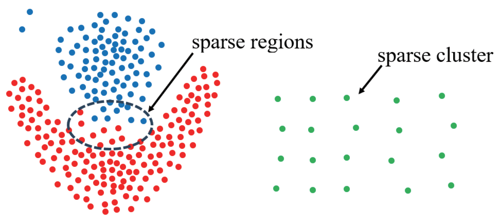
DCM calculation. As illustrated in
Figure 3 in
Section 1, this hybrid metric not only maintains the ability to identify sparse clusters but also alleviates issues related to weak connectivity, thereby enhancing the effectiveness of the clustering algorithm. Specifically, the algorithm operates in two steps: First, it computes the
DCM value and
value for each data point. Using the
DCM values, it performs an initial classification, dividing the points into core point candidates and boundary point candidates. Then, the core candidate set is further refined by leveraging the
values. Specifically, if a point within the candidate set for internal points has a relatively low
value, it is determined not to be an internal point. This screening process is applied to the candidate set, effectively distinguishing internal points from boundary points. Compared to traditional directional-center clustering methods, the incorporation of
effectively mitigates weak connectivity issues. Meanwhile, in contrast to conventional density-based clustering, the directional-center assessment based on
DCM values demonstrates superior performance in identifying sparse clusters. Under our proposed distributed computing framework, once the data partitioning is complete, the
and
DCM values for data points within each partition can be computed independently, without requiring inter-node communication.
3.2.1. Computation of DCM
Based on
DCM, data points are categorized as either boundary points or internal points. To achieve this, the
DCM values for all data points in dataset
P must first be computed. The calculation method for
DCM values is provided in Equation (
1) in
Section 2.1. As indicated by the formula, the computation of
DCM requires identifying the
k-nearest neighbors (KNNs). The primary computational cost of the DEALER algorithm lies in the distance calculations involved in finding KNN points, which represents the bottleneck that constrains the speed of the clustering process. When the dataset size becomes large, the time complexity of
for these calculations becomes prohibitively expensive. Thus, improving the algorithm’s speed is essential to meet the demands of large-scale data processing. To accelerate KNN searching, this section proposes a filtering strategy based on a
z-value filling curve, referred to as the Z-CF (
z-value-based computing filter) algorithm. Before introducing the Z-CF algorithm, we first prove two theorems.
Theorem 1. In a d-dimensional space, given two data points and , where , , the following holds: Proof. For two data points,
and
, where
,
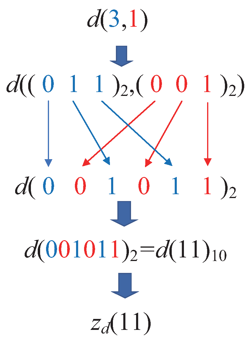
, we refer to the method described in Lemma 4 of reference [
14], which rearranges the coordinate values by alternating between the most significant bit and the least significant bit to derive the
z-value of a point. This implies that
. □
Theorem 2. Given two data points p and q in a d-dimensional space, if the distance between them , then the following holds: Here, and are new data points derived by subtracting and adding s to each coordinate value of the data point p, respectively. That is, and .
Proof. If , then for , it holds that . Based on Theorem 1, we can conclude that . □
Since data points, when mapped from high-dimensional space to one-dimensional space via the z-value filling curve, cannot be guaranteed to be ordered strictly by distance, it is necessary to first identify the potential range for the KNN points, then compute the distances within that range and sort the points to obtain the exact KNN. Building on the two theorems mentioned above, after arranging the data points in ascending order based on their z-values, we can efficiently identify the KNN points for any given data point p. This is achieved by iteratively searching in both forward and backward directions along the z-value axis, selecting the closer of the two candidate points at each step. After k iterations, we obtain a point , and it follows that the distance is necessarily greater than the farthest distance among p’s true KNN points. According to Theorem 2, the positions of p’s KNN points along the z-value axis fall within a specific range. Furthermore, Theorem 2 establishes that p’s KNN points must lie within a neighborhood centered at p with a radius of after k comparisons. Within this defined range, an exact KNN search can then be conducted. Compared to traditional KNN searches, incorporating the z-value index significantly reduces the search space by narrowing the potential candidate set from the entire dataset to a localized subset. This approach substantially decreases the number of distance computations required, thereby improving computational efficiency. The detailed strategy and analysis are presented as follows.
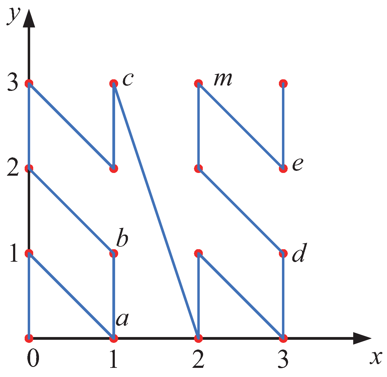
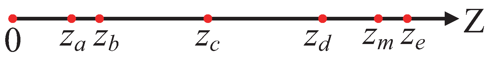
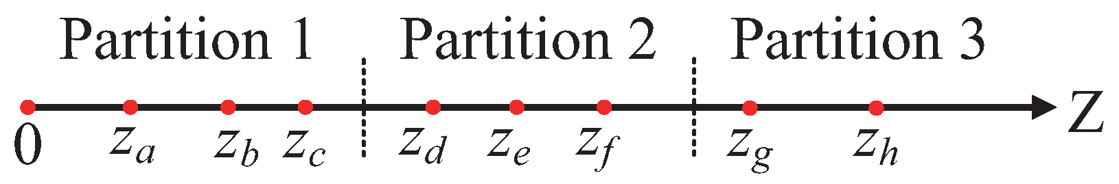
First, identify the initial potential KNN points. For a given d-dimensional dataset P, all data points in the dataset are mapped into one-dimensional space via the z-value filling curve so that the z-value coordinates correspond one-to-one with the original space coordinates. Next, the data points are sorted by their z-values. On the z-value axis, the initial potential KNN points are identified. For any data point p, search for one point in each direction along the z-value axis: one in the positive direction, denoted , and one in the negative direction, denoted . The distances between p and these two points, and , are calculated. The point with the smaller distance is selected as the first initial KNN point. Then, along the direction of the closer point on the z-value axis, search for the second point, calculate the distance, and compare it with the previously identified farther point. The point with the smaller distance is selected as the second initial KNN point, and this process continues until k points are identified.
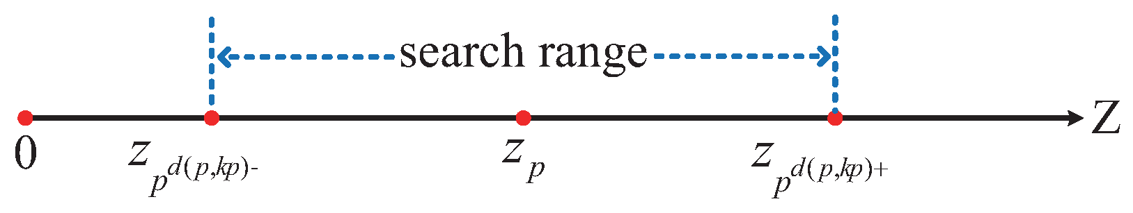
Next, determine the potential range for the KNN points. For any given data point p, the initially identified KNN points are sorted in ascending order of distance. The point that is the k-th closest, denoted as , is selected. The potential range for the KNN points is defined as a neighborhood centered at p with a radius of .
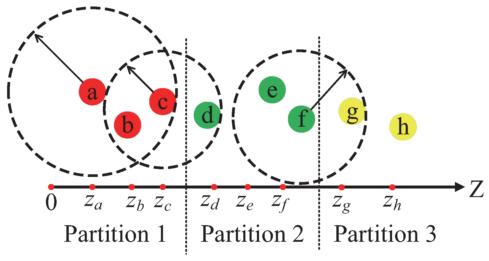
As illustrated in
Figure 9, instead of performing a search over the entire data space, a one-dimensional linear search within the interval
is sufficient to identify the KNN points of data point
p. This is because, for any data point
q such that
, according to Theorem 2, the
z-value of
q must lie within the interval
. Therefore, there is no need to compute the distances from
q to
p for the ranges where
or
, as it is guaranteed that
will be greater than
.
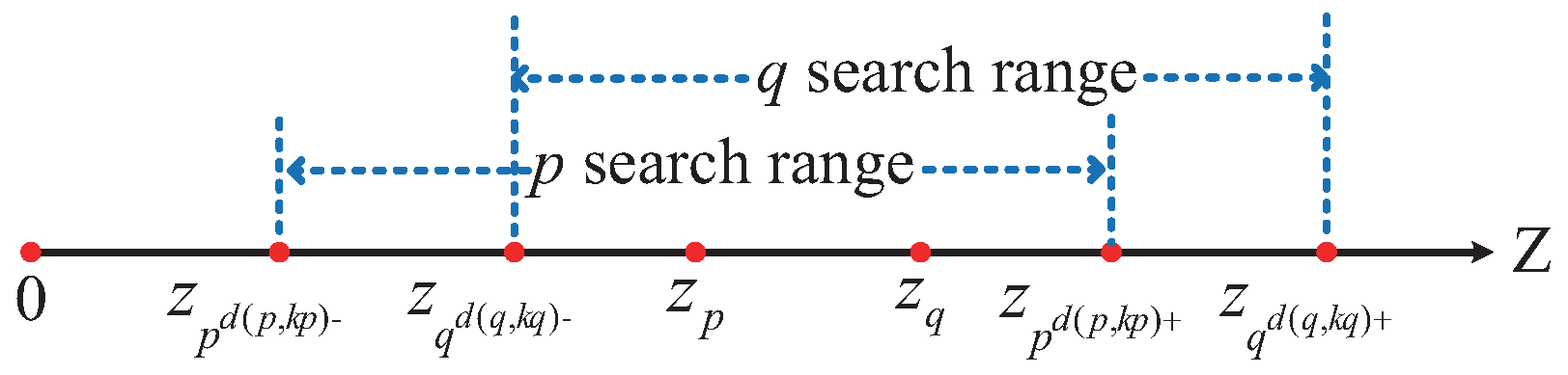
It is important to note that if, for data points
p and
q, the
lies within the interval
, and the
lies within the interval
, then when calculating the KNN for data point
p, the distance
needs to be calculated once. Similarly, when calculating the KNN for data point
q, the distance
must also be calculated once. This results in redundant distance calculations and increases unnecessary computational overhead, as illustrated in
Figure 10.
To optimize the computational strategy and reduce unnecessary overhead, this study adopts a one-sided computation approach. Specifically, for a given data point
p, we calculate the distance only to the points on one side of the interval. This means either computing the distance to the data points in the right-hand interval
or to those in the left-hand interval
. Both methods yield the same result, and in this paper, the first method is employed, as shown in
Figure 11.
The proposed strategy is based on Theorem 3.
Theorem 3. Given a dataset P and any data point p, suppose there exists a subset such that for , . The subset is then divided into two subsets, denoted as and , where . For , , and for , . Then, we have the following: Proof. According to Theorem 2, for all
, we have
. Since
, it follows that
, thus proving Equation (
6). A similar argument can be applied to prove Equation (
5). □
Based on Theorem 3, when calculating the distance between data point p and data point q, if , we can compute the distance from p to . Similarly, when calculating the distance from p to with respect to their previous data points in the interval , we can compute the distance from p to all . This reduces the computational load, making the Z-CF algorithm more efficient.
The Z-CF algorithm uses the z-value filling curve to map points from high-dimensional space into one-dimensional space. The z-value filling curve ensures that points that are close in the original space remain close in the one-dimensional space, thereby narrowing the KNN search range. To further reduce redundant calculations, a one-sided calculation strategy is employed to optimize the algorithm. The specific computational process of the Z-CF algorithm is described in Algorithm 1.
| Algorithm 1 Z-CF |
| Input: Dataset P, KNN value k |
| Output: KNN sets and distances for all points in P |
| 1: Transform all data points into one-dimensional space using Equation (2) to obtain |
| 2: Sort the data points by their z-values in ascending order |
| 3: |
| 4: for each data point in do // Find the initial KNN points |
| 5: // Q represents the subset of P with removable points |
| 6: |
| 7: while do |
| 8: , |
| 9: |
| 10: |
| 11: |
| 12: |
| 13: end while |
| 14: Sort by increasing distance in |
| 15: |
| 16: end for |
| 17: for each data point in do |
| 18: Compute and |
| 19: for such that do |
| 20: if then |
| 21: |
| 22: Update |
| 23: end if |
| 24: if then |
| 25: |
| 26: Update |
| 27: end if |
| 28: end for |
| 29: end for |
3.2.2. Computation of
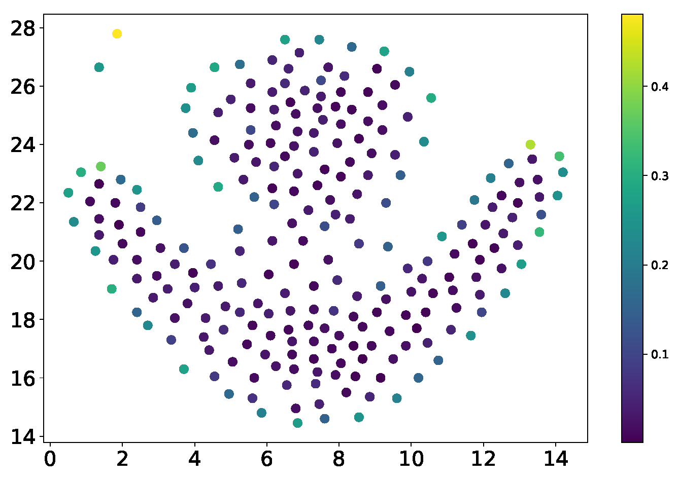
Although clustering methods based on DCM values ensure the identification of sparse clusters, they perform poorly in addressing weak connectivity issues. To maintain the capability of identifying sparse clusters while mitigating weak connectivity problems, a hybrid metric incorporating the -value is introduced. Unlike traditional density computation methods, the calculation of the -value in the DEALER algorithm does not require specifying a neighborhood radius. Instead, it directly uses the reciprocal of the Euclidean distance between a data point and its k-th nearest neighbor, as determined during the DCM computation process, to represent the data point’s density. This approach offers two key advantages. First, it does not introduce additional computational overhead, as it merely applies a reciprocal operation to pre-computed data. Second, the reciprocal of the distance to the k-th nearest neighbor is positively correlated with the density as traditionally defined: the greater the distance to the k-th neighbor, the smaller the reciprocal, indicating sparser surrounding points and lower density in sparse regions, and vice versa. Moreover, using the reciprocal of the distance to the k-th nearest neighbor as a density metric inherently normalizes the density, which facilitates subsequent data processing tasks, such as data filtering. The formal definition of density is provided as follows:
Definition 3 (K-Nearest Neighbor Limited Density). For any data point , if denotes the k-th nearest neighbor of in the data space, then the reciprocal of the Euclidean distance between and is defined as the k-nearest neighbor limited density of the data point .
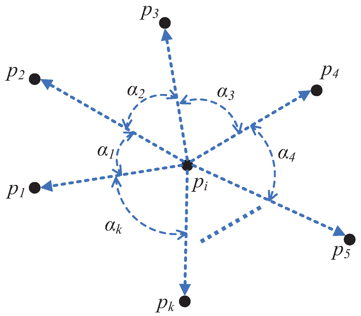
Figure 12 illustrates the density computation process. As shown, for a given data point
, assuming
, five nearest neighbors can be identified, denoted as
, and sorted by distance in ascending order as
. Based on
Figure 12, the formula for calculating the density of
is presented in Equation (
7):
Here, represents the density of the data point , is the k-th nearest neighbor of in the data space (corresponding to point in the figure), and denotes the Euclidean distance between and .
Based on the above analysis, to accurately differentiate between boundary points and core points and further enhance clustering accuracy, it is necessary to classify data objects using a combination of two metrics: density () and local DCM. Within the same cluster, boundary points generally have lower density compared to core points, while their DCM values are higher. Since the core points uniquely determine a cluster, it is essential to ensure all core points are correctly identified. To achieve this, a two-step strategy is employed: first, data objects are filtered based on their DCM values, followed by a secondary filtering based on density values. Specifically, data objects in the dataset are divided into two subsets based on their DCM values: a core point candidate set and a boundary point candidate set. Next, density values are applied to further filter the objects in the core point candidate set. If the density of a data object is smaller than the densities of more than half of its k-nearest neighbors (KNNs), the object is reclassified as a boundary point. This approach is justified because, for objects in the core point candidate set, their KNN points are relatively evenly distributed. If the density of a data object is exceeded by a certain proportion (, typically set to 50%) of its KNN points, the object is likely closer to the cluster boundary. Consequently, the center of the cluster to which this object belongs is biased toward the region with higher-density data points. This methodology provides a clear distinction between core points and boundary points within the dataset, laying a solid foundation for subsequent clustering operations.


