Analysis the Composition of Hydraulic Radial Force on Centrifugal Pump Impeller: A Data-Centric Approach Based on CFD Datasets

Abstract

Centrifugal pumps are essential in various industries, where their operational stability and efficiency are crucial. This study aims to analyze the composition and variation characteristics of the hydraulic radial force on the impeller using a data-centric approach based on computational fluid dynamics (CFD) datasets, providing guidance for optimizing impeller design. A high-precision CFD simulation on a six-blade end-suction centrifugal pump generated a comprehensive hydraulic load dataset. Data analysis methods included exploratory data analysis (EDA) to uncover patterns and trigonometric function fitting to model force variations accurately. Results revealed that the hydraulic radial force exhibits periodic behavior with a dominant blade passing frequency (BPF), showing minimal fluctuations at the rated flow rate and increased fluctuations as flow deviates. Each blade’s force could be approximated by sine curves with equal amplitudes and frequencies but successive phase changes, achieving high fitting quality (R² ≥ 0.96). The force on the impeller can be decomposed into the contributions of each blade, with symmetric blades canceling out the main harmonics, leaving only constant terms and residuals. This study provides insights into force suppression mechanisms, enhancing pump stability and efficiency, and offers a robust framework for future research on fluid–structure interactions and pump design.

1. Introduction

As the most widely applied type of pump equipment, centrifugal pumps perform work on liquid media by relying on the high-speed rotation of the impeller, thus achieving the transportation and pressurization of the liquid. Operational economy and stability are the two most crucial considerations in the design and manufacturing process of centrifugal pumps [1,2]. With the development of modern industry, the requirements for pump performance in various fields are constantly increasing. The design of modern centrifugal pumps is continuously evolving toward higher rotational speeds, larger flow rates, and higher heads [3,4,5]. Curved blades, accompanied by the high-speed rotation of the main shaft, generate more significant multi-wall shear rotational turbulence. This intensifies the rotational, transient, and nonlinear characteristics of the flow within the pump, leading to increasingly prominent complex unsteady flow phenomena such as the interaction between the rotating and stationary parts, flow separation, wake-jet flow, and secondary flow inside the centrifugal pump [6,7,8,9,10].

The unsteady flow within the pump under high energy density conditions generates significant radial forces which primarily result from circumferential pressure asymmetry induced by impeller–volute interactions. These forces drive shaft deflection, accelerate bearing wear, and elevate vibration and noise levels through fluid–structure interactions. This leads to an increase in the deflection of the main shaft, an acceleration of bearing wear, and an elevation in the levels of vibration and noise. In severe cases, it may even cause the blades to break, thus having a highly detrimental impact on the operational stability of the pump unit [11,12,13,14]. Additionally, the periodic hydraulic impact of unsteady flow on dynamic and static sealing components such as the sealing rings may disrupt the original installation and fitting relationships, increase mechanical friction and sealing clearances, and exacerbate the internal leakage of the fluid medium. Ultimately, this results in a decrease in volumetric efficiency and mechanical efficiency and an increase in the energy consumption level during the operation of the pump [15,16,17,18]. Therefore, a large number of researchers have initiated studies on unsteady flow phenomena inside centrifugal pumps, analyzing the formation mechanism and dynamic characteristics of the hydraulic induction effect on the impeller, so as to provide effective guidance for the weakening and suppression of the hydraulic induction effect.

The hydraulic load acting on the impeller inside a centrifugal pump consists of two parts: the axial force and the radial force. The axial force can be transmitted via thrust bearings and actively balanced through methods such as balance discs and balance holes [19,20,21]. However, the radial force cannot be simply balanced, but rather weakened and suppressed through the optimized design of the stator geometry and other key components in the hydraulic model [22]. A large number of scholars have conducted research on the variation laws of the hydraulic radial force on the impeller and its influencing factors, thereby providing theoretical guidance for the design and operation of centrifugal pumps. Zhang et al. [23,24] showed, through experimental measurements and numerical simulations, that the hydraulic radial force acting on the impeller mainly originates from the pressure pulsation and uneven pressure factors within its internal flow field. It has the characteristic of periodic variation with constantly changing magnitude and direction and is closely related to the operating conditions, such as the flow rate.

In recent years, a large amount of research has focused on optimizing the geometric structure of the hydraulic model to effectively suppress the hydraulic radial force. The fluid domains inside a centrifugal pump can generally be divided into three parts: the suction part, the volute, and the impeller. The geometric structures of these three components all have a direct impact on the magnitude and fluctuation level of the hydraulic radial force on the impeller. Regarding the suction chamber, Wang et al. [25] carried out a numerical simulation of the internal flow field of a double-suction centrifugal pump with a semi-spiral suction chamber. They proposed that adding a baffle in the suction chamber can reduce the pressure pulsation amplitude within the impeller and the overall radial force exerted on the impeller. In terms of the volute, Zhou et al. [26] found that after changing the geometric shape of the single volute to a double one, the radial force and pulsation amplitude on the impeller during the starting process of the centrifugal pump can be effectively reduced. At the rated rotational speed, the radial force can be reduced by approximately 80%. However, the vector distribution of the radial force for the double volute type is more complex and disordered than that of the single volute type. Due to the complex shape of the impeller blades that rotate at high speeds, many researchers have focused on design improvements for the impeller structure. For example, Song [27] et al. compared the influences of single-suction and double-suction impellers on pressure oscillation and radial force, respectively. The results showed that the double-suction impeller can promote a relatively uniform flow at its outlet and alleviate the interaction effect between the impeller and the volute, thus effectively weakening the hydraulic radial force on the impeller. In addition, adjusting the hub size [28], the tip clearance [29], and the key size parameters of the blades such as the blade thickness, outlet angle, and curvature [30] are also important means to achieve the suppression of the hydraulic radial force on the impeller.

Although a large number of studies have been conducted on the evolution laws and fluctuation characteristics of the hydraulic radial force on the centrifugal pump impeller under different flow conditions and different structures and have provided certain theoretical guidance for the suppression of the hydraulic radial force on the impeller in the field of engineering design, most existing studies regard the impeller as a whole.

A multitude of studies have delved into the evolution laws and fluctuation characteristics of the hydraulic radial force acting on the centrifugal pump impeller under diverse flow conditions and various structural setups. These studies have furnished theoretical guidance for the suppression of the impeller’s hydraulic radial force within the realm of engineering design. Nonetheless, the majority of existing research endeavors consider the impeller as an integrated entity. By means of computational fluid dynamics (CFD) technology, they predict the hydraulic radial force of the impeller under different structural and operating condition schemes, so as to help designers screen out better schemes. In many industrial application scenarios, although the above-mentioned “design-simulation-iteration” process has achieved certain improvement effects in reducing the force level, limited by the complex and changeable time-frequency characteristics of the hydraulic radial force on the impeller, it is unable to deeply reveal the internal relationship between the local flow field excitation and the overall radial force characteristics. As a result, the relevant optimization design work lacks sufficient pertinence and efficiency.

Based on the logical framework driven by data, this paper takes an end-suction centrifugal pump as the research object. Through high-precision CFD simulation, an impeller hydraulic load dataset covering multiple operating conditions is constructed, and the composition mechanism and variation characteristics of the hydraulic radial force of the centrifugal pump impeller are analyzed through data analysis and mining. The prioritization of this investigation stems from two critical needs: (1) to establish explicit connections between localized flow excitation patterns (e.g., pressure pulsations, vortex shedding) and the resultant global radial force characteristics, which are essential for suppressing vibration-induced failures in industrial pump systems; and (2) to demonstrate how a data-centric methodology—specifically, the systematic mining of a physics-informed CFD dataset—can reveal force decomposition principles that traditional analyses often overlook, thereby providing a generalizable framework for impeller optimization.

In the subsequent content, Section 2 introduces the research object and the detailed process of obtaining the dataset relying on CFD simulations. Section 3 expounds on the data analysis framework and process. Section 4 gives the analysis and a discussion of the research results. Section 4 provides a summary of the composition law of the radial force and its engineering application implications, followed by the conclusion in Section 5.

2. Numerical Simulation

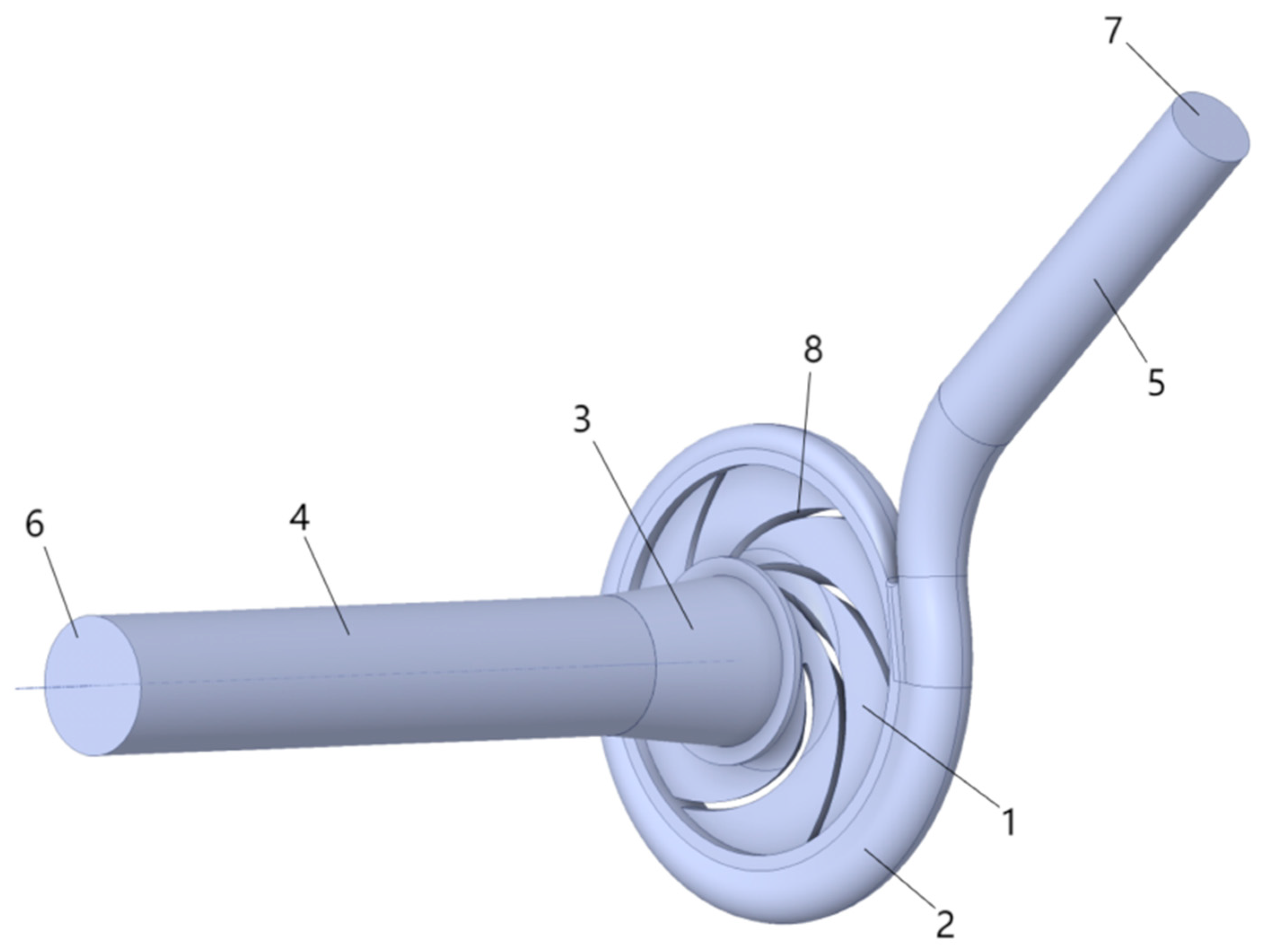
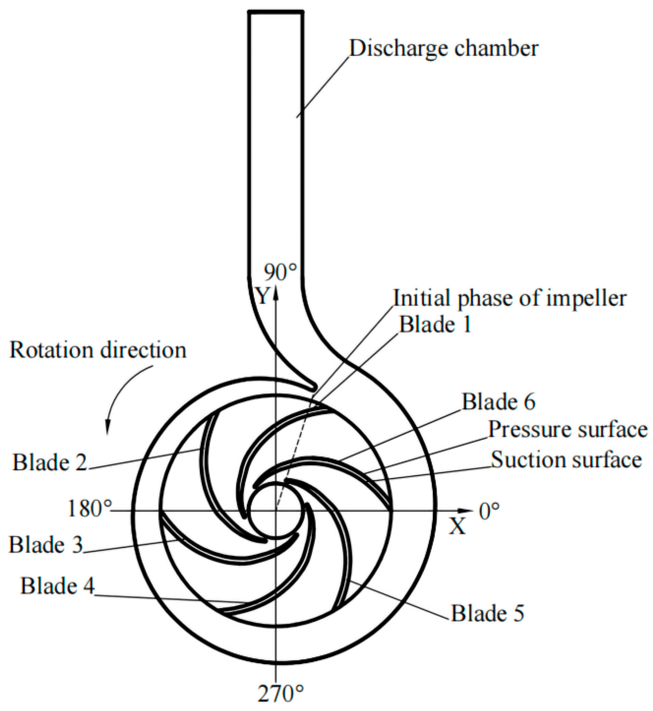
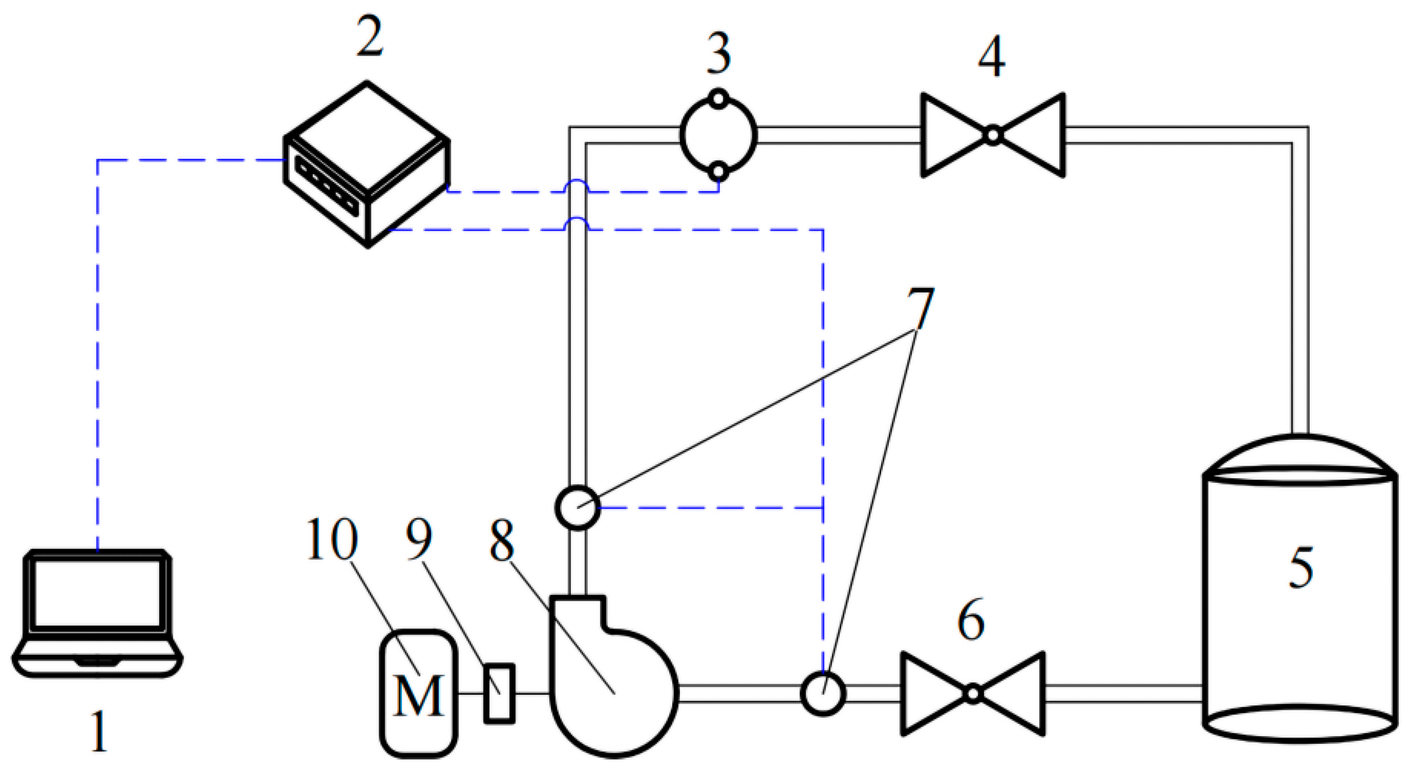
2.1. Research Object

The research object selected in this paper is a horizontal end-suction centrifugal pump with six blades, designed for transporting clear water medium at room temperature. This centrifugal pump is manufactured by Hunan Credo Pump Co., Ltd. Xiangtan, China. Its main structural and performance parameters are listed in

Table 1. Main structure and performance parameters of the research object.

Parameter	Symbol	Value
Rated flow	Qd	12.5 m3/h
Rated head	Hd	22.7 m
Rated speed	nd	2900 r/min
Specific speed	Ns	2.97
NPSH required	NPSHr	4.0 m
Impeller inlet diameter	D1	0.061 m
Impeller outlet diameter	D2	0.139 m
Impeller outlet width	b2	0.007 m
Number of blades	N	6
Volute base diameter	D3	0.15 m
Pump inlet diameter	D4	0.05 m
Pump outlet diameter	D5	0.032 m

. The structural design and performance configuration of this pump are carefully optimized to meet the requirements of practical applications, ensuring its reliability and efficiency in the process of transporting clear water medium.

The hydraulic model is extracted based on the three-dimensional structural assembly of this centrifugal pump, as shown in Figure 1. The fluid domain inside the centrifugal pump is mainly divided into three parts: the impeller region, the suction chamber, and the discharge chamber.

In order to ensure that the fluid flowing into and out of the computational domain is fully developed for sufficient computational accuracy, the inlet and outlet parts of the pump are extended to form the inlet pipe and the outlet pipe. The lengths of the inlet and outlet pipes are each five times their respective diameters. This pipe extension design can effectively mimic the actual flow conditions at the pump’s inlet and outlet, minimizing the impact of boundary conditions on the calculation results and enhancing the reliability and accuracy of the computational analysis of the centrifugal pump’s internal flow field.

To more clearly illustrate the impeller structure of the research object and its relative relationship with the volute, the mid-section of the impeller and volute regions in Figure 1 is intercepted, as shown in Figure 2. In Figure 2, a Cartesian rectangular coordinate system is established with the central position of the impeller as the coordinate origin. The axial direction of the impeller is defined as the Z direction (perpendicular to the paper plane and not drawn in the figure), while the X and Y directions are defined as the two radial directions of the impeller.

Meanwhile, the rotational position of the impeller—when a straight line is formed by connecting the root of a certain blade (Blade 5 in the figure), the center point of the impeller, and the protruding point at the end of the tongue—is defined as its initial phase. This initial phase also serves as the initial moment for the calculation of the unsteady flow field within the centrifugal pump.

2.2. Governing Equations and Turbulent Model

The CFD research in this work mainly focuses on the three-dimensional incompressible unsteady flow problems within a centrifugal pump under different flow rate conditions and is solved by applying the Reynolds-Averaged Navier-Stokes (RANS) method. The solution process is based on the continuity equation and the Navier–Stokes equation:

$${\displaystyle \frac{\partial \rho }{\partial t}}+\nabla ·\left(\rho \stackrel{⃑}{u}\right)=0$$

(1)

$${\displaystyle \frac{\partial \left(\rho \stackrel{⃑}{u}\right)}{\partial t}}+\nabla ·\left(\rho \stackrel{⃑}{u}\stackrel{⃑}{u}\right)=-\nabla P+\nabla ·\left[\mu \left(\nabla \stackrel{⃑}{u}+{\left(\nabla \stackrel{⃑}{u}\right)}^T\right)\right]+\stackrel{⃑}{f}$$

(2)

where t is time (s); $\overrightarrow{u}$ and p represent the velocity vector (m/s) and static pressure (Pa), respectively; ρ and µ stand for density (kg/m³) and effective viscosity (kg/(m·s)), respectively; and $\stackrel{⃑}{f}$ is external body force term (N/m³). The effective viscosity μ in Equation (2) combines the molecular viscosity μL and turbulent eddy viscosity μ_t, i.e., μ = μ_l + μ_t. For the SST k-ω turbulence model used in this study, the turbulent eddy viscosity μ_t is calculated based on the turbulent kinetic energy k and specific dissipation rate ω, as detailed in [31].

To close the above two major governing equations and meet the solution requirement, a suitable turbulence model needs to be supplemented. Considering that the high-speed rotating impeller with complex twisted blades inside the centrifugal pump generates a strong fluid shear effect and has a high Reynolds number, this study selects the SST k-ω turbulence model proposed by Menter [31]. This turbulence model combines the advantages of both the k-ε model and the k-ω model. In the calculation of turbulent viscosity, it takes into account the transport of turbulent shear stress, improving the prediction accuracy for separated flows and flows with adverse pressure gradients. Therefore, it has been widely applied in predicting the internal flow field of centrifugal pumps [28,32,33].

The core idea of the SST k-ω model lies in using a blending function to achieve the transition from the high Reynolds number turbulent core region far from the wall to the low Reynolds number region near the wall:

$$\phi =F_1{\phi }_1+{(1-F_1)\phi }_2$$

(3)

where F₁ is the factor of function and $\phi$ is the coefficient of the SST k-ω turbulence model, while ${\phi }_{1 }$, and ${\phi }_2$ stand for coefficients of the k-ω turbulence model and k-ε turbulence model, respectively.

For the region far away from the wall, the flow turbulence is solved solely by the k-ε turbulence model, and the factor F₁ is set to 0. Conversely, in the region close to the wall, the factor F₁ is set as 1. This is to more accurately consider the influence of viscous forces on turbulence, thereby more precisely capturing the development and dissipation phenomena of turbulence near the boundary layer.

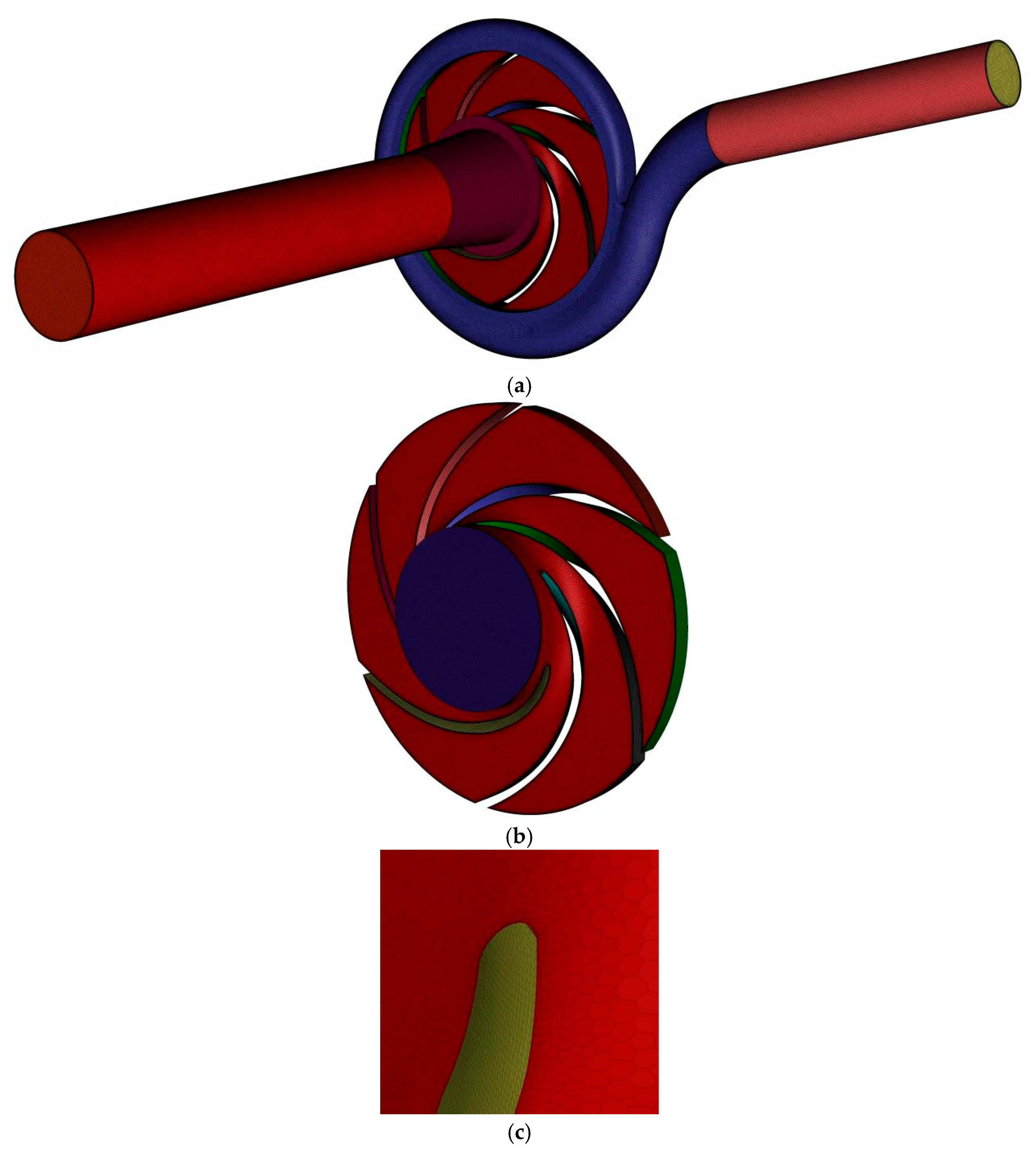
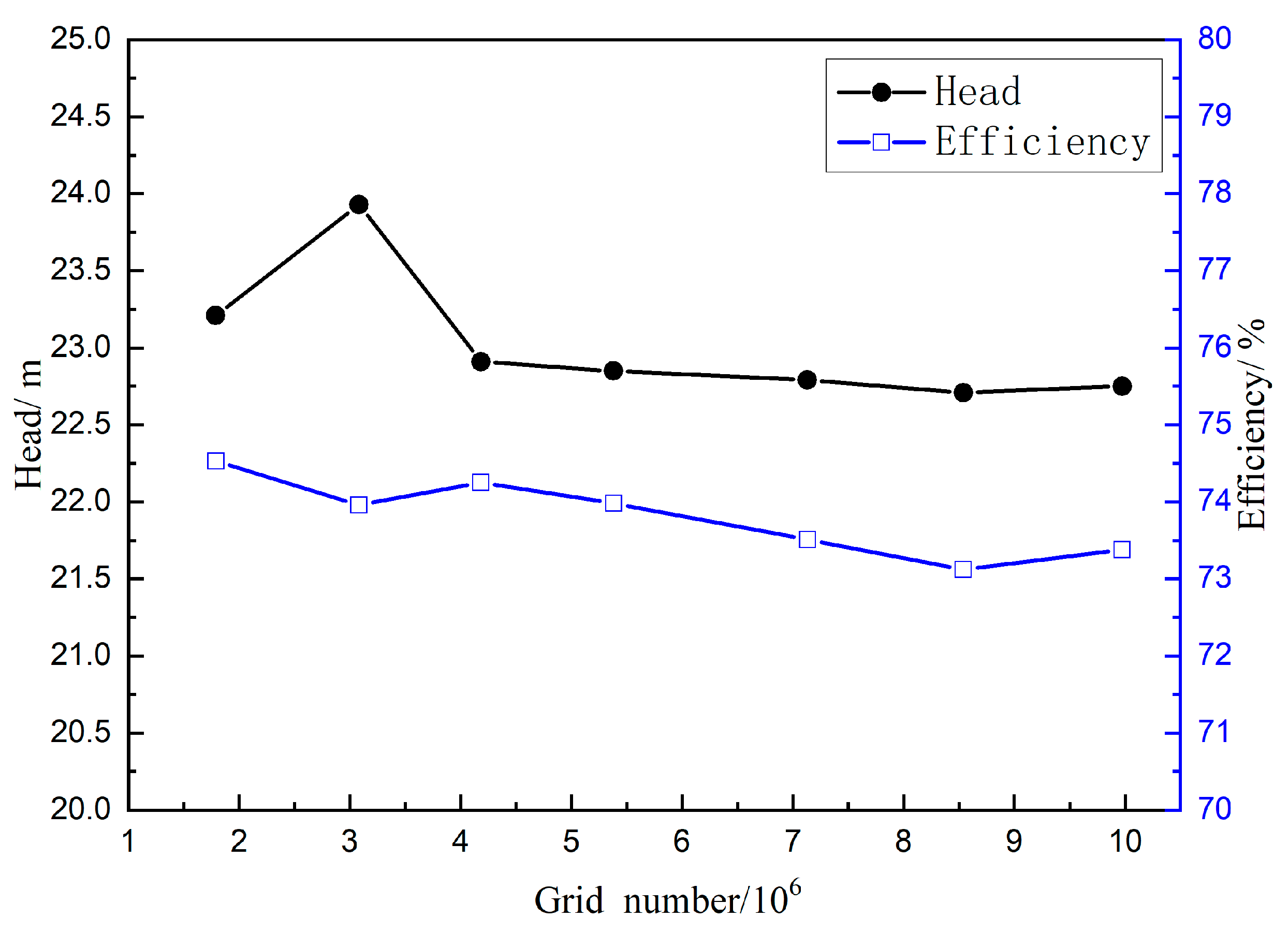
2.3. Mesh Generation and Independence Verification

The Fluent Meshing 2024 software module is selected to generate the meshes for the entire fluid domain of the centrifugal pump. As depicted in Figure 3, the meshing process adopts the Poly-hexcore meshing method based on the “Mosaic” technology. Specifically, hexahedral elements with eight nodes are used to fill most of the internal flow field region. Meanwhile, high-quality stratified multi-prismatic elements are maintained in the boundary layer, and then general polyhedral elements are automatically employed to connect these two types of elements. This meshing approach has prominent advantages, such as strong adaptability in terms of mesh connection, high solution efficiency and accuracy, and good meshing flexibility.

At the same time, local refinement is carried out for regions with complex shapes and structures, such as the volute tongue. Additionally, multiple layers of boundary layer elements are applied to resolve the near-wall flow, with the first-layer grid height calibrated to maintain an average y+ < 20 across all surfaces. In regions prone to strong flow separation (e.g., the impeller domain), additional grid refinement is implemented to achieve y+ < 10, ensuring accurate resolution of adverse pressure gradients and vortex shedding dynamics. For example, Figure 3a shows the overall grid of the fluid domain, and Figure 3c shows the mesh refinement and the boundary layer meshes in the root region of the blade, which is indicated by the dashed box in Figure 3b.

To evaluate the influence of the grid size on the calculation accuracy, the changes in the two key external characteristic parameters of the centrifugal pump, namely, the head and the efficiency, under the rated flow condition are observed as the total number of meshes varies, as shown in Figure 4. It is easy to find from the figure that when the number of grids is less than 5.4 × 10⁶, the fluctuations in the predicted results are quite significant, and the fluctuation range of the head is as high as 1.1 m. However, when the number of grids exceeds 7.1 × 10⁶, both the head and the efficiency remain stable, and the fluctuation ranges of these two parameters remain within 0.1m and 0.4%, respectively.

Therefore, to balance both the solution accuracy and efficiency, a meshing scheme with a total number of elements of approximately 8.5 × 10⁶ is finally selected. The average mesh quality of this scheme is 0.91, and the numbers of elements and nodes in each fluid domain are listed in

Table 2. Number of elements and nodes in each fluid domain.

Fluid Domain	Element Number	Node Number
Inlet pipe	1,093,640	2,806,035
Suction region	423,445	1,089,239
Impeller region	2,349,537	6,029,682
Discharge chamber	4,224,759	10,842,508
Outlet pipe	447,719	1,157,567
Total	8,539,100	21,925,031

.

2.4. Boundary Conditions and Solver Settings

The commercial software ANSYS Fluent 2023R2 is employed to solve the unsteady flow field inside the centrifugal pump under five different flow conditions, i.e., 0.8Q_d, 0.9 Q_d, 1.0 Q_d, 1.1 Q_d, and 1.2 Q_d, while Q_d is the rated flow listed in Table 1. The rotational speed of the impeller remains constant at 2900 r/min for each flow condition.

For each flow condition, a steady-state calculation is first conducted to provide the initial flow field for the unsteady calculation. In the steady-state calculation, the fluid medium is set as water at room temperature, with a density of 998.2 kg/m³ and a dynamic viscosity of 1.006 × 10⁻³ Pa·s. A velocity inlet condition is applied at the pump inlet, and the velocity magnitude is calculated based on the flow rate under the corresponding condition and the pump inlet area. The outflow boundary condition is imposed at the outlet pipe termination to emulate hydrodynamically developed free-stream conditions. This configuration is physically justified by the extended discharge section (see Figure 1), which provides sufficient flow development length to dampen flow asymmetries induced by the impeller’s rotational effects. The “outflow” boundary condition optimizes centrifugal pump simulations by focusing computation on critical regions (impeller/volute), preventing artificial outlet constraints from distorting upstream flow.

The Multiple Reference Frame (MRF) model is used to handle the flow in the impeller region. The mesh of the impeller itself is treated as a stationary grid region, and the centrifugal effect due to its high-speed rotation is considered through an inertial coordinate system. A stage average condition is applied at the interface between the impeller region and the stator regions (such as the suction chamber and volute) to exchange flow field information, including velocity and pressure distribution. All wall surfaces are set with a “no-slip” condition. Referring to the manufacturer’s process standards, the inner wall surfaces of the suction chamber and volute are given a roughness of 100 µm, while the rest wall surfaces are set to a roughness of 50 µm. Meanwhile, a standard wall function with semi-empirical formulas is used in the near wall region. This function simplifies the calculation and effectively connects the flow field in the near wall viscous sub-layer and the turbulent flow in the main flow region.

The Semi-Implicit Method for Pressure Linked Equations (SIMPLE) algorithm is used for the solution. It is a semi-implicit pressure-velocity coupling algorithm that corrects the velocity and pressure fields by constructing a pressure correction equation, ensuring that the calculated velocity field satisfies the continuity equation. For each governing equation, a root mean square (RMS) convergence accuracy of 10⁻⁴ is specified for computational convergence.

The results of the steady-state calculation are used as the initial conditions for the unsteady calculation. Meanwhile, on the basis of the steady-state calculation settings, the MRF model is disabled, and the dynamic mesh technology is adopted. The impeller region is set as “Mesh motion” to accurately simulate the real flow in the impeller region. To ensure the convergence and stability of the unsteady calculation, the total duration of the calculation is 0.1655 s, corresponding to eight impeller rotation cycles, and only the calculation results of the last two impeller rotation cycles are used for subsequent result analysis. The time step of the calculation is 1.1494 × 10⁻⁴ s, corresponding to the time taken for the impeller to rotate 2°.

All calculations are performed on a Lenovo workstation platform (CPU: 7R32, RAM: 128 GB). The total calculation time for each flow condition case (including one steady-state calculation and an eight rotation cycle of unsteady calculation) is approximately 80 h.

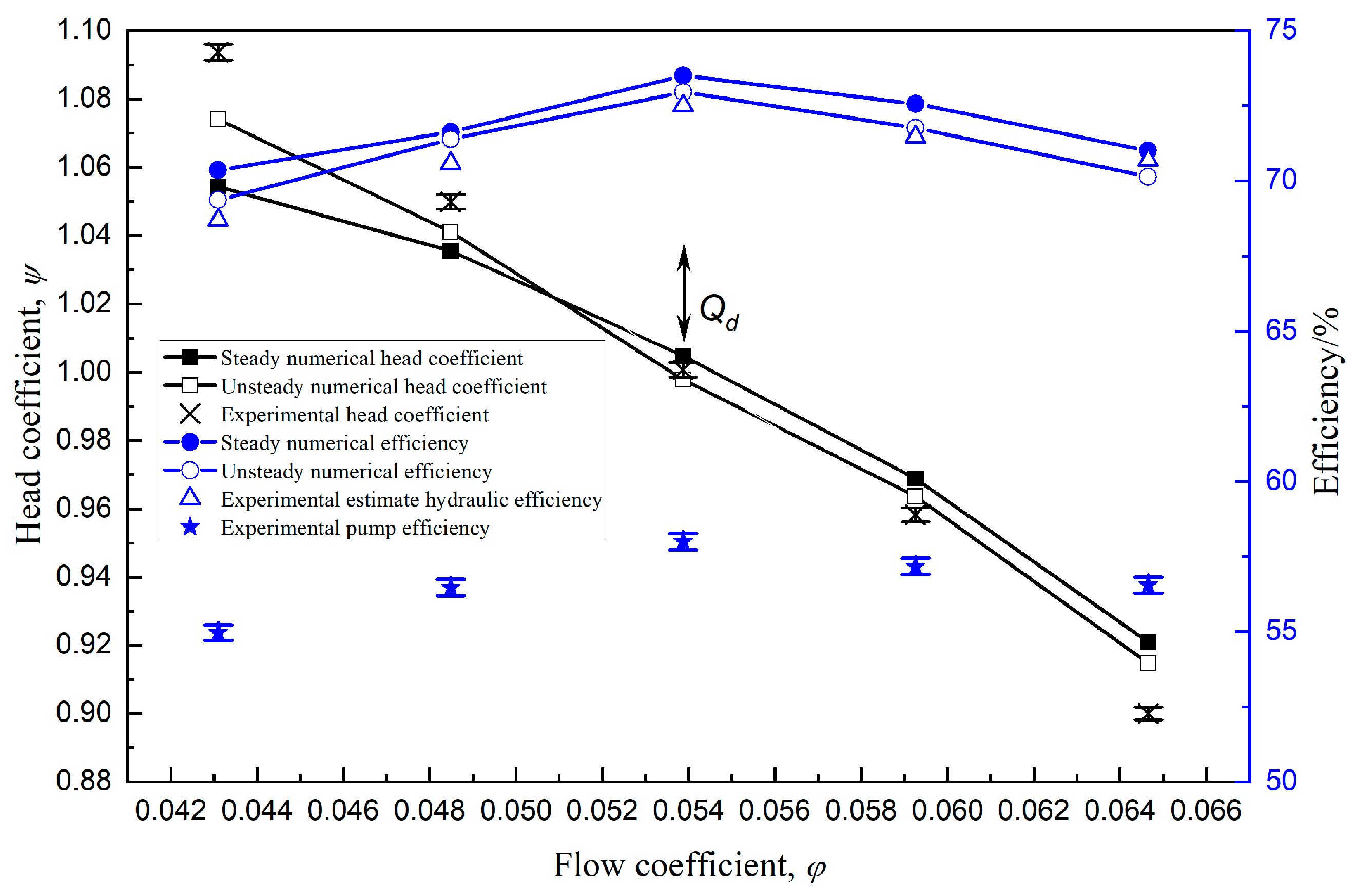
2.5. Experimental Validation

As shown in Figure 5, referring to the level 1 accuracy class in standard ISO 9906-2012 [34], the external characteristic curves of the centrifugal pump are tested on a closed-loop test rig. The test system mainly consists of two parts: a closed-loop fluid circuit composed of a centrifugal pump, a water tank, inlet and outlet valves, and several pipes; and a signal measurement and acquisition facility composed of pressure gauges, electromagnetic flowmeter, and data acquisition card, etc.

During the experiment, the water temperature is maintained at 20 ± 1 °C, and the rotational speed of the centrifugal pump is kept at 2900 ± 5 r/min using a frequency converter. The inlet valve is always fully open, and the outlet valve opening is adjusted to ensure the stable operation of the device under different flow conditions. An electromagnetic flowmeter (Model: CKLDG-D50-X, accuracy: ±0.2%) is used for flow measurement, and the pressure gauge for pressure measurement has an accuracy of ±0.1%. The head under each flow condition is calculated from the readings of two pressure gauges located at the inlet and outlet of the centrifugal pump:

$$H={\displaystyle \frac{P_2-P_1}{\rho g}}+{\displaystyle \frac{{V_2}^2-{V_1}^2}{2g}}+Z$$

(4)

where P₂ and P₁ are the pressure at the outlet and inlet of the pump, respectively; V₂ and V₁ are the velocity at the outlet and inlet of the pump, respectively; ρ is density of water; g is gravitational acceleration; and Z is the height difference between the pressure gauge installation positions at the inlet and outlet pipe sections. The values of V_out and V_in are obtained by dividing the measured flow rate by the cross-sectional area of the outlet and inlet, respectively.

Furthermore, the efficiency under each flow condition is calculated based on the above calculated head and shaft power:

$$\eta ={\displaystyle \frac{\rho g{Q}_{v}H}{P_S}}$$

(5)

where H, Q_v, and P_s are the head, flowrate, and shaft power of the pump, respectively. The shaft power is measured by a torque meter with a measurement accuracy of ±0.1% and a frequency converter.

The systematic error of the experiment is controlled within 0.15%. Through an uncertainty analysis, the uncertainties of the head and efficiency are determined to be 0.21% and 0.38%, respectively. Finally, the numerical results and experimental measurement results under each flow condition are compared, as shown in Figure 6. In Figure 6, the flow rate and head values are dimensionless, converted into the flow coefficient φ and the head coefficient Ψ, respectively.

The experimental measurements plotted with error bars in Figure 6 represent the total pump efficiency obtained through physical testing. It should be noted that while the CFD simulations specifically predict hydraulic efficiency η_h, the experimentally measured total efficiency η inherently combines three components: η = η_h × η_v × η_m, where η_v denotes volumetric efficiency, and η_m mechanical efficiency. To enable direct comparisons between simulation predictions and experimental data, the estimated hydraulic efficiency values are derived from measurements by applying the following relationship: η_he = η/(η_v × η_m). This combined volumetric–mechanical efficiency factor (η_v × η_m) is established at 80% through a systematic evaluation of the manufacturer-provided engineering datasets, which integrate decades of operational performance records from equivalent pump configurations across diverse industrial applications. The value reflects validated correlations derived from accumulated field test data rather than theoretical assumptions, adhering to industry-standard efficiency characterization protocols that account for typical wear patterns and manufacturing tolerances observed in production hardware.

It can be seen from Figure 6 that the deviation between the head values predicted by the steady-state numeration and the experimental measurements is controlled within 3.60%, while the deviation between the head values predicted by the unsteady numeration and the experimental measurements is 1.80%, i.e., only half of that of the steady-state numeration. The maximum deviations between the efficiency values predicted by the steady-state and unsteady numerations and the estimate experimental measurements under each flow condition are 1.65% and 0.81%, respectively. Further analysis reveals that at the rated flow rate Q_d, both the steady-state and unsteady numerations can achieve high prediction accuracy. However, the greater the deviation of the flow rate from the rated point, the larger the deviation between the calculation results and the experimental values; this phenomenon is particularly obvious in the low flow conditions. Taking the head coefficient as an example, at the rated flow rate Q_d, the deviations between the steady-state and unsteady numerations and the experimental values are 0.40% and 0.28%, respectively. At a lower flow rate of 0.8 Q_d, these deviations increase to 3.60% and 1.80%, respectively.

Overall, the numerical calculations in this study are highly reliable, and the unsteady numeration can provide better prediction accuracy than the steady-state numeration, especially in the low flow rate conditions. This is because under low flow rate conditions, the internal flow field of the centrifugal pump is complex, with unsteady phenomena such as backflow, vortices, boundary layer separation and reattachment, strong pressure pulsation, and significant interaction between the impeller and volute [25,35]. These phenomena are ultimately reflected in the external characteristic parameters, such as the head and efficiency, and can only be accurately captured by an unsteady numerical model with real rotation of the impeller mesh during the solving process.

2.6. Dataset from CFD

This study focuses on analyzing the composition mechanism and variation characteristics of the hydraulic radial force on the centrifugal pump impeller through data analysis and mining. The dataset is derived from the numerical results of the unsteady flow field inside the centrifugal pump under five different flow conditions: 0.8Q_d, 0.9Q_d, 1.0Q_d, 1.1Q_d, and 1.2Q_d.

During the unsteady solving process, the calculation information is collected and stored every time step. After the solving is completed, only the results of the last two cycles are retained to ensure the accuracy and reliability of the data.

Ultimately, a dataset consisting of five data files, namely 0.8Q_d.csv, 0.9Q_d.csv, 1.0Q_d.csv, 1.1Q_d.csv, and 1.2Q_d.csv, is compiled. Each data file mainly contains information on result parameters such as the solve step number, time, hydraulic forces on the entire impeller as well as the various parts of it, inlet and outlet pressures, torque, etc.

The dataset primarily comprises time-series records of hydraulic forces (F_y, F_x) acting on distinct impeller surfaces, including individual blade profiles, along two orthogonal axes (X and Y). These force vectors are derived through numerical integration of surface pressure distributions in their respective directions. The orthogonal decomposition of hydrodynamic radial forces is implemented primarily to facilitate analytical procedures and computational processing, given the intrinsic vector nature of these dynamic loads. This approach is further justified by the critical role of hydraulic radial forces in governing rotor system deformations and vibration mechanisms in centrifugal pumps, where both experimental investigations and dynamic analyses in these fields conventionally require orthogonal directional measurements to ensure the proper characterization of fluid–structure interactions [11].

3. Data Analysis Method

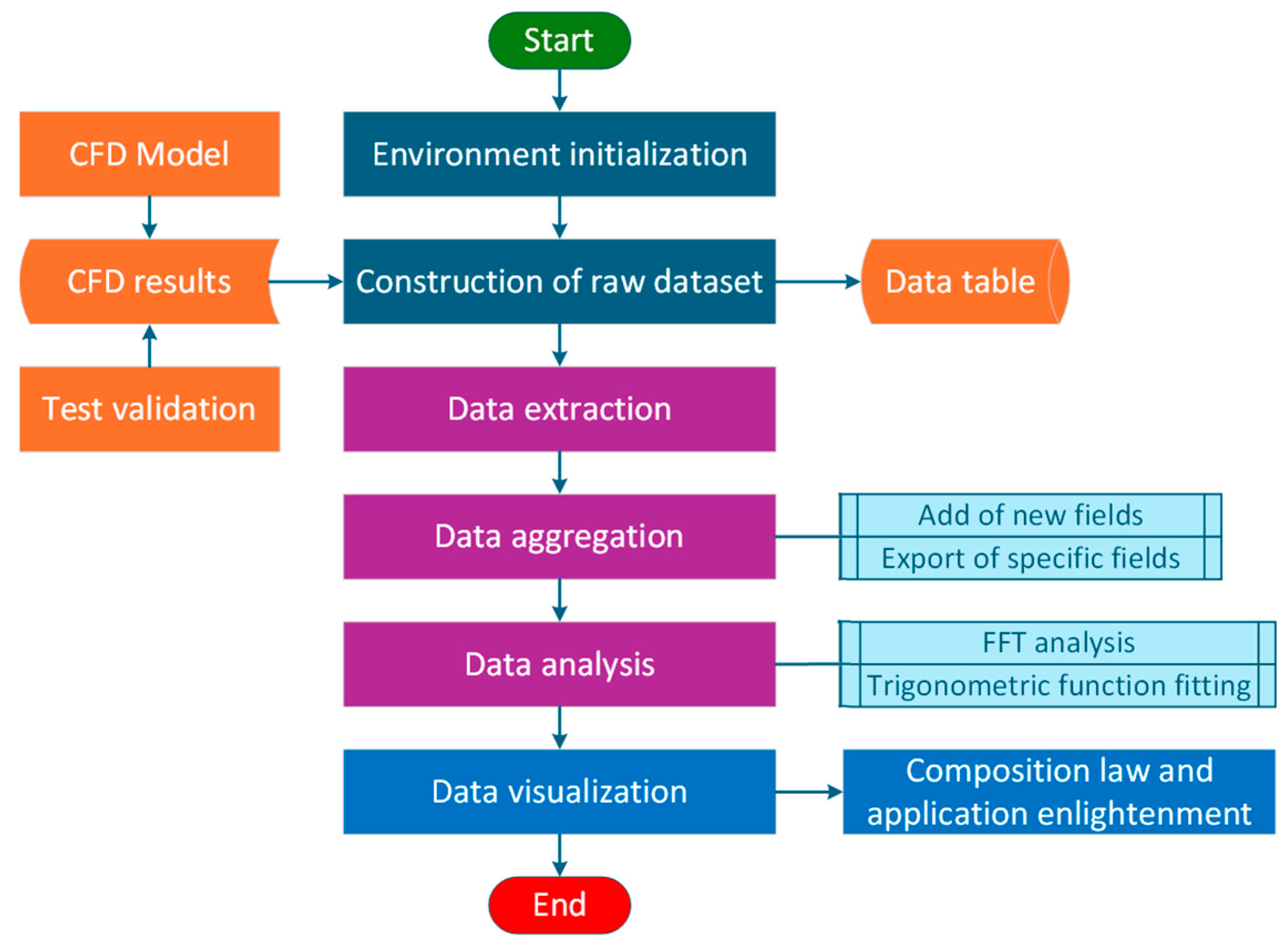
3.1. Basic Procedure

Based on the dataset obtained from the unsteady CFD numerations, a program for data analysis, mining, and visualization was developed using Matlab R2022a software. A flowchart of the program is illustrated in Figure 7.

As shown in Figure 7, the initialization of the data analysis environment is carried out first. The numerical analysis results under various flow conditions are read in the form of data tables to construct a raw dataset, with the dataset generation explicitly incorporating CFD model and test validation components (see Section 2.2, Section 2.3, Section 2.4 and Section 2.5) as foundational inputs. The data analysis is conducted within the Exploratory Data Analysis (EDA) framework [36]. That is, functions such as indexing and screening are first used to extract specific data fields, and the basic characteristics of the data are observed through simple visual plotting. Subsequently, data aggregation is performed, where new fields are added and specific fields are exported according to the research requirements, further enriching the data structure. Finally, data analysis and mining are carried out, including applying Fast Fourier Transform (FFT) analysis to explore the frequency characteristics of relevant parameters and using trigonometric function fitting to uncover the potential variation patterns of certain variables. When the data analysis is completed, the data are visualized for better understanding, with a new module composition law and application enlightenment appended to the workflow to highlight the derivation of physical insights and their specific engineering implications.

It should be noted that the source code in the Supplementary Materials of this paper covers the entire process of data analysis, including data visualization, to facilitate its invocation and analysis by researchers and engineering designers. While the source program provides data visualization plots, it also separately exports the original data involved in the plotting, thus enabling the use of third-party tools for independent plotting or other analytical processing of the data.

3.2. Key Algorithms

Since the original dataset is derived from the unsteady CFD analysis, the data analysis and mining mainly involve FFT analysis and trigonometric function fitting algorithms.

FFT is an efficient algorithm for computing the DFT (Discrete Fourier Transform), which is widely used in fields such as digital signal processing. The FFT algorithm is based on the decomposability of DFT. It achieves fast computation by decomposing the DFT of a long sequence into multiple DFTs of short sequences. In this study, a dedicated FFT function named “FFT_plot_and_export” is developed using the Decimation in Time (DIT) algorithm. The basic idea is as follows: for a discrete time sequence x[n] (n = 0, 1, …, N − 1) of length N, assuming N is an integer power of 2, the sequence is first split into two subsequences of length N/2 according to the parity of the time order. Then, with the help of specific rotation factors, the DFT result of the original sequence is represented as a combination of the DFT results of these two subsequences. Subsequently, the parity decomposition operation is repeated on the obtained subsequences until the length of the subsequence becomes 2. Since it is easy to compute the DFT of a subsequence of length 2, the DFT result of the original sequence can be efficiently calculated through such step by step decomposition and computation. The detailed principle of the DIT algorithm can be found in [37].

The “lsqcurvefit” function in MATLAB is used for trigonometric function fitting of the time varying curves of relevant parameters. The maximum number of iterations in the fitting process is set to 10,000, and the convergence tolerance is 10⁻⁶. The “lsqcurvefit” function is used to solve the nonlinear least squares curve fitting problem. Its goal is to find a set of function parameter values that minimize the sum of the squared residuals between the given nonlinear function and the observed data. Specifically, the Levenberg-Marquardt algorithm is adopted during the fitting process using this function. This algorithm is a commonly used nonlinear least squares optimization algorithm that combines the advantages of the gradient descent method and the Gauss-Newton method. It has good convergence and stability when dealing with nonlinear least squares problems. The specific principle can be found in [38].

4. Results and Discussion

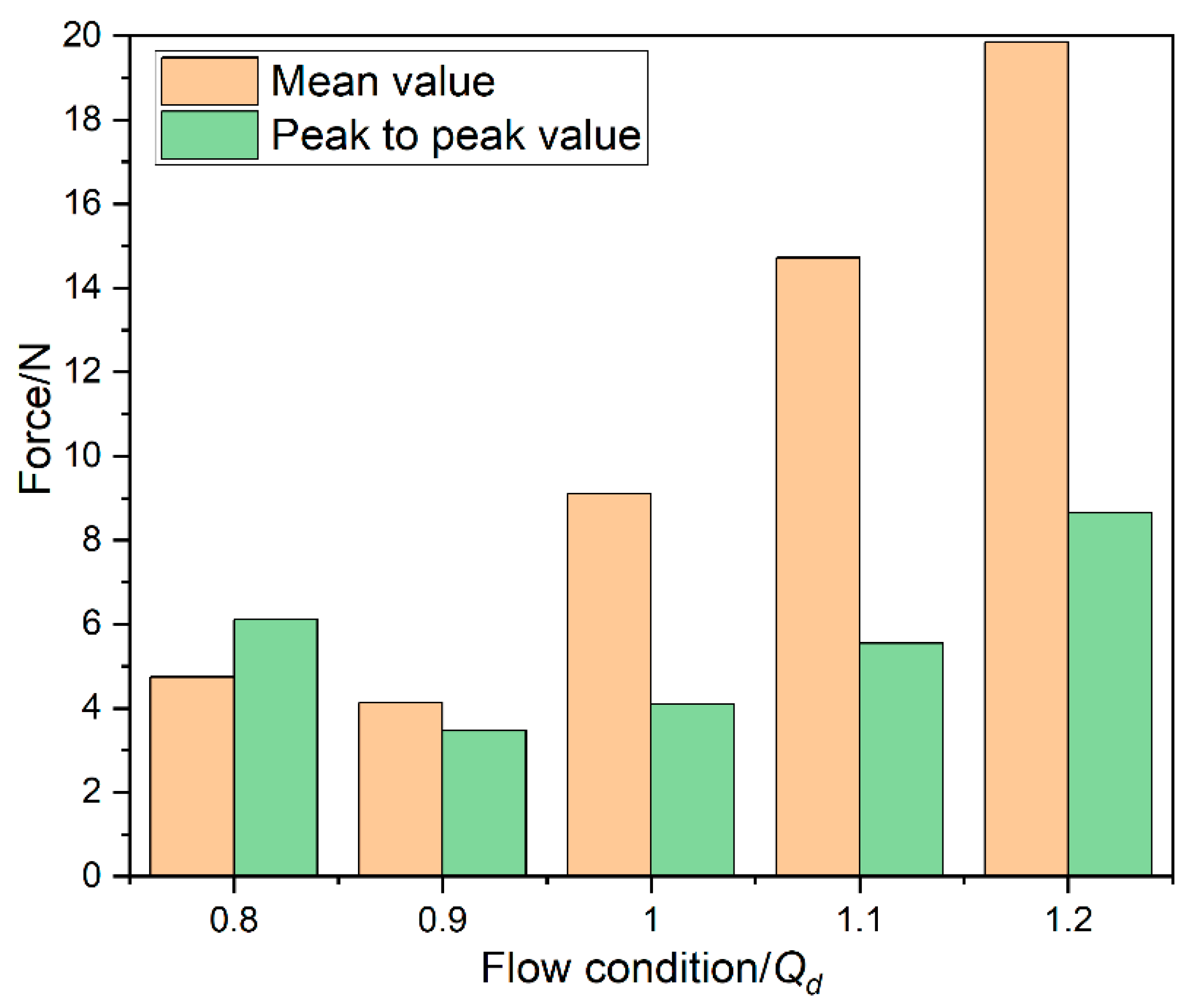
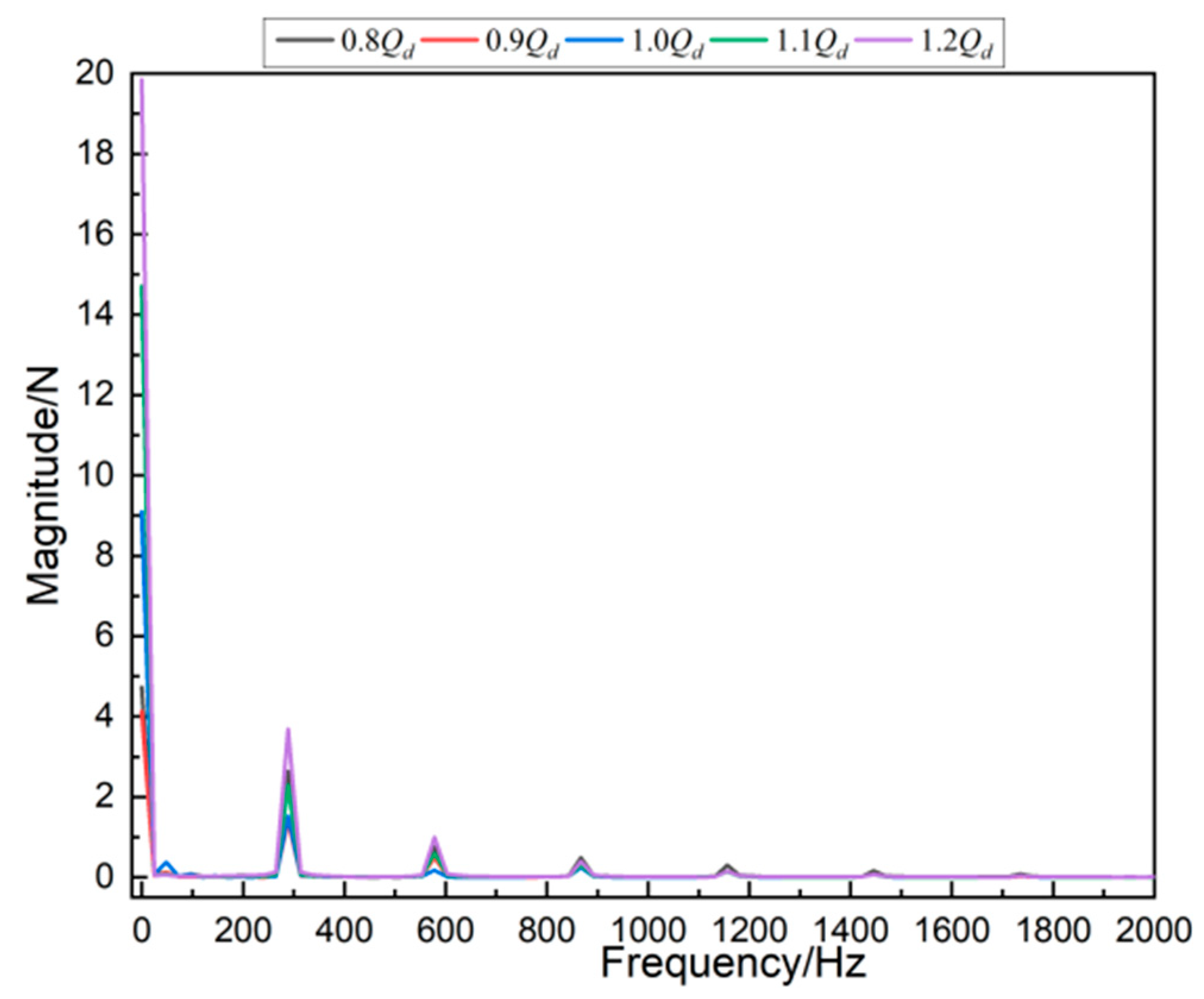
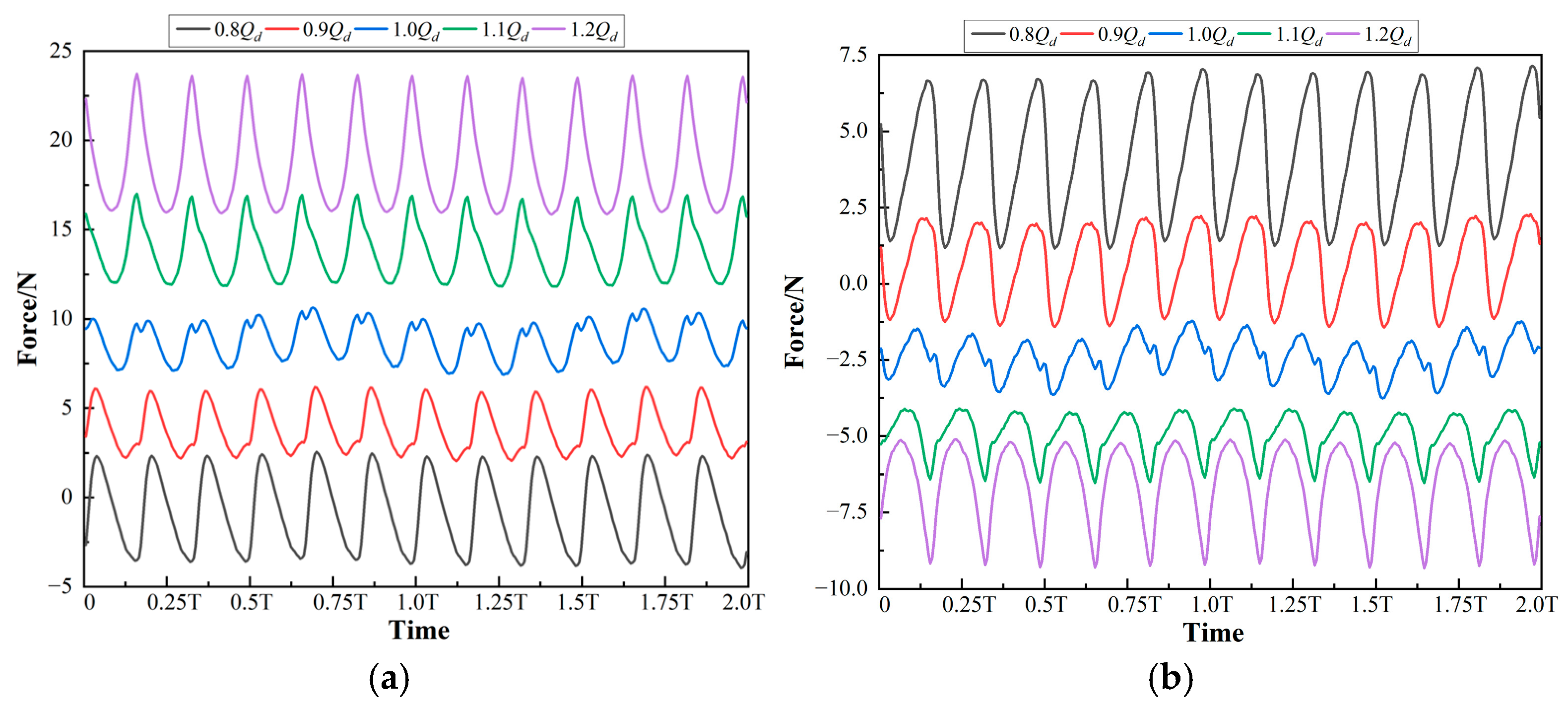
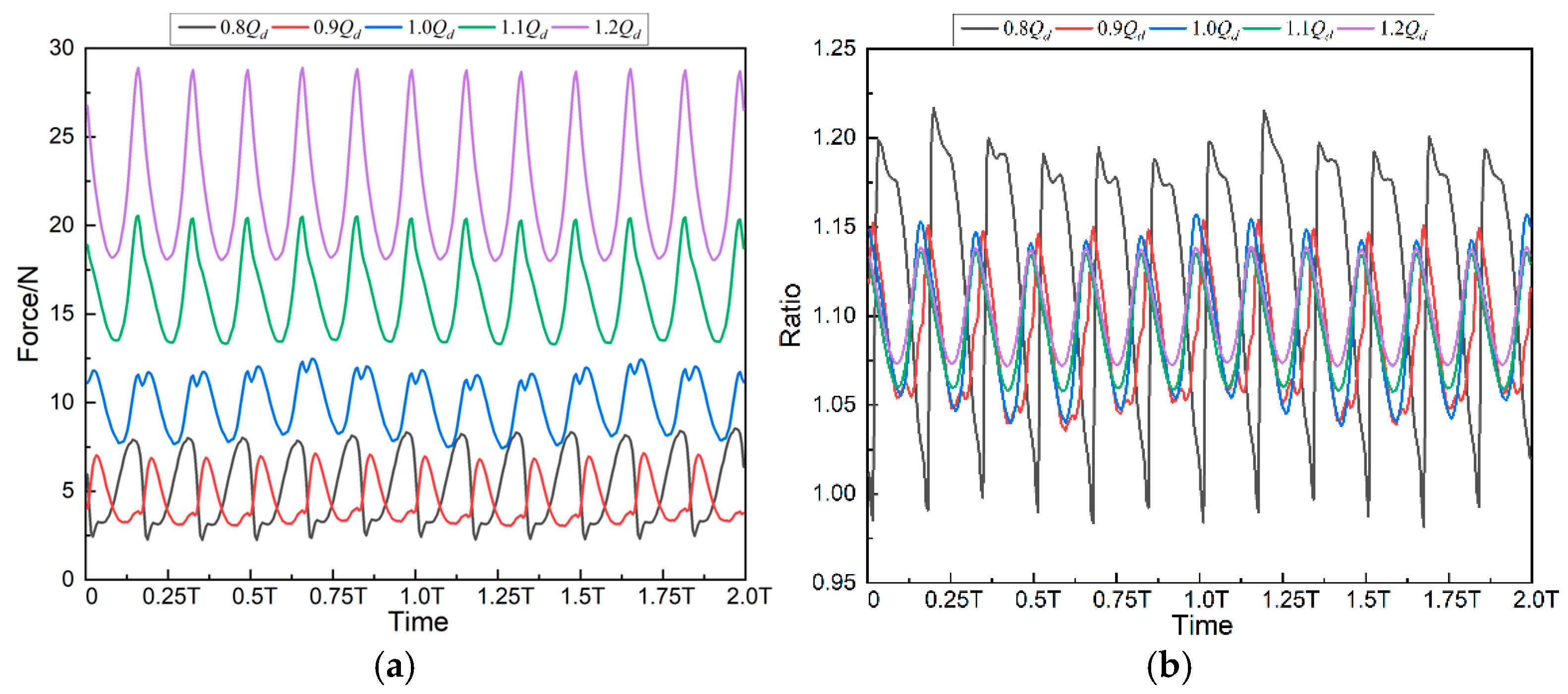
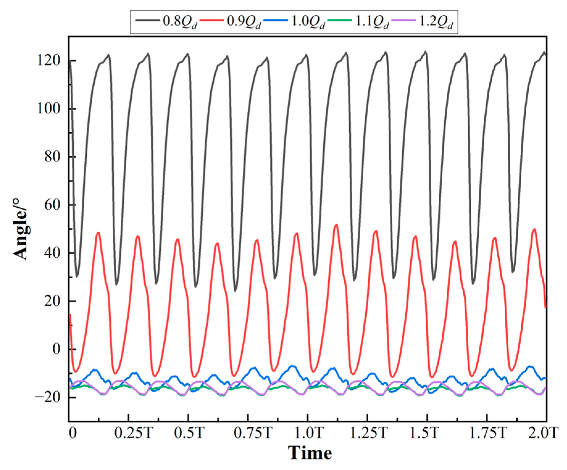
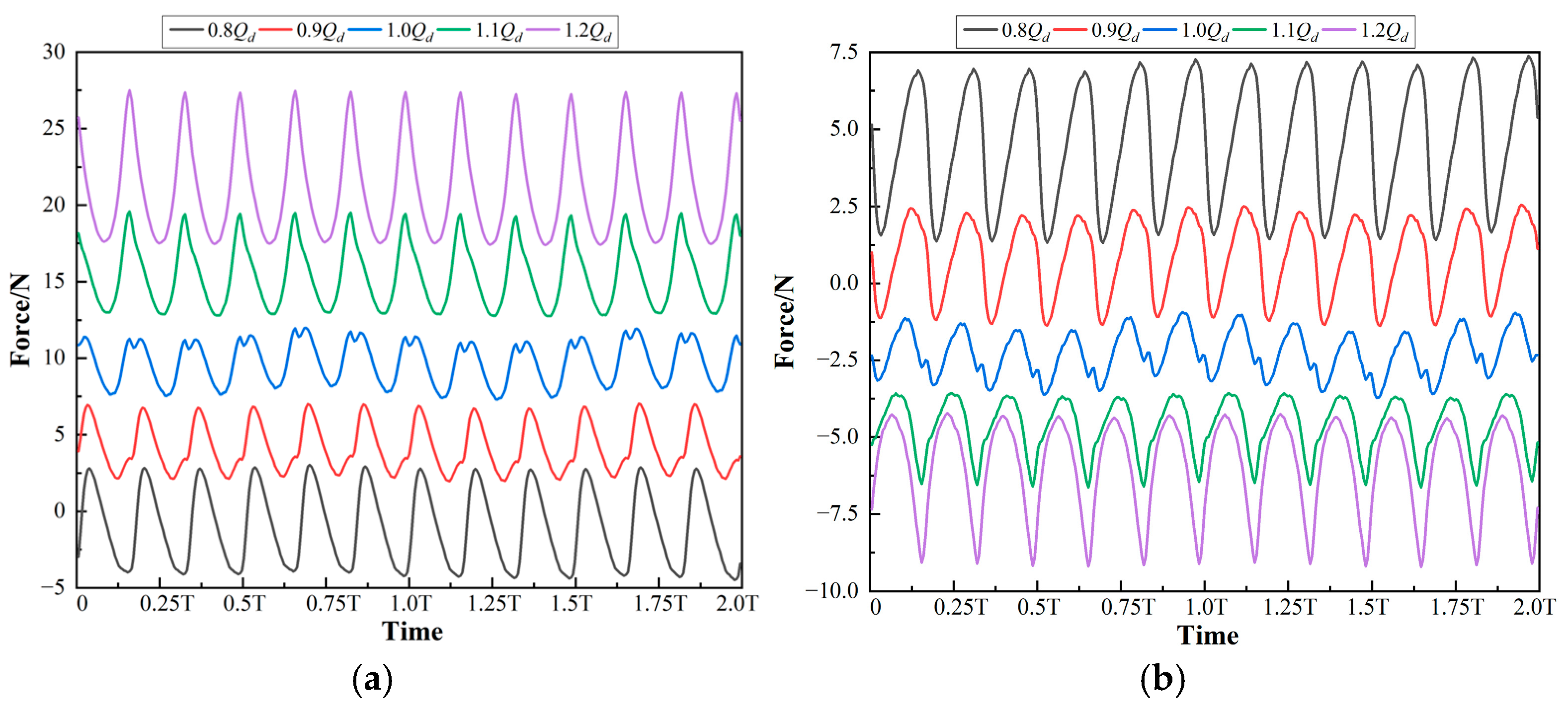
4.1. Hydraulic Force on the Whole Impeller

Firstly, following the common practice reported in existing literature, the impeller is regarded as a whole. The hydraulic radial force and hydraulic axial force acting on the impeller within two impeller rotation cycles under different flow conditions are plotted, as shown in Figure 8a,b, respectively. For all the plots of time-series data in this paper, including Figure 8, the time is uniformly represented by the multiple of the impeller rotation cycle. One impeller rotation cycle, that is, 1.0T, corresponds to approximately 0.0207 s.

As shown in Figure 8, as the flow rate increases, both the hydraulic radial force and hydraulic axial force acting on the impeller generally show an increasing trend, which is consistent with the findings of Yang et al. [39] and Dong et al. [40]. Meanwhile, the hydraulic axial force on the impeller under each flow condition remains basically stable, with a very limited fluctuation range, and its magnitude is also much lower than that of the hydraulic radial force. A possible explanation for the trend of the hydraulic axial force is that the liquid in the impeller changes its flow direction from the axial direction to the radial direction, and the momentum of the liquid also changes accordingly. An increase in the flow rate means that the mass of the liquid passing through the impeller per unit time increases, so the rate of change of the liquid momentum also increases. Correspondingly, the reaction force exerted by the liquid on the impeller, that is, the axial force, also increases.

However, compared with the hydraulic axial force, the variation behaviors of the hydraulic radial force are more complex. The statistics of the average value and peak-to-peak value of the time-varying curve of the hydraulic radial force under each flow condition are determined; the results are plotted in Figure 9. It can be observed that near the rated flow rate, both the average value and peak-to-peak value of the hydraulic radial force are relatively small, and the minimum values of both occur under the flow condition of 0.9Q_d. The further away from the rated flow rate, the larger the average value and peak-to-peak value will be, and the level of the hydraulic radial force under the high flow condition is higher than that under the low flow condition. Furthermore, it can also be seen from Figure 8a that under relatively low flow conditions (0.8Q_d~1.0 Q_d), the curves of the hydraulic radial force show a pattern of obvious waveforms superimposed on small waveforms, while when the flow rate is relatively high (1.1Q_d and 1.2Q_d), there are basically only large waveforms.

To obtain the dominant frequency of the fluctuations, a FFT analysis is performed for the hydraulic radial force curves in Figure 8a; the results are shown in Figure 10. It is evident that under all flow conditions, the blade passing frequency (BPF) is the dominant frequency of the fluctuations, superimposed with the shaft frequency and other multiples of the BPF, which is consistent with other research reports [41,42].

Moreover, the hydraulic radial force on the impeller under each flow condition is decomposed into two components of the X-axis and Y-axis directions, as shown in Figure 11a,b, respectively. The time varying curves of these two components exhibit similar fluctuation characteristics: the fluctuation is minimal at the rated flow rate, and it increases as the flow rate deviates from the rated value. Additionally, the waveforms under larger flow conditions are smoother than those under smaller flow conditions.

Figure 12 shows the variation of the angle of the hydraulic radial force on the impeller with time under different flow conditions. In this paper, the angle of the hydraulic radial force θ is defined as follows:

θ = arctan2(F_y, F_x)

(6)

In the formula, F_x and F_y represent the X direction and Y direction components of the hydraulic radial force, respectively. The “arctan2” function is an extension of the arctangent function in mainstream programming languages such as Matlab. Upon receiving the abscissa and ordinate of a point in the Cartesian coordinate system, it determines the directed angle (with a value range of (−π, π]) between the line connecting the point to the origin and the positive X axis. This calculation is based on the positive or negative values and magnitudes of F_x and F_y, using the rules associated with the arctangent function. Thus, it can more accurately determine the direction of the angle. For ease of observation, the unit of radians in the figure is converted to degrees.

Figure 12 indicates that, apart from the significant variations in the amplitude and fluctuation level of the hydraulic radial force, there are also substantial differences in its angle under different flow conditions. Overall, its angle varies less under the rated and high flow conditions, indicating more stable flow. In contrast, under low flow conditions such as 0.8Q_d and 0.9Q_d, the angle fluctuates much more significantly.

The above phenomena can be explained by the unsteady flow inside the centrifugal pump under different flow conditions. At the rated flow rate, the incoming flow at the impeller inlet matches well with the blade inlet angle. The flow adheres to the blade surface without significant flow separation or backflow, and the flow directions at the volute and impeller outlet are also well matched. As a result, both the time average values of hydraulic radial force and the pulsation amplitude are small. When the flow rate is low, the velocity at the impeller inlet decreases, leading to significant flow separation on the blade suction surface and the formation of a local low pressure area. This causes backflow and exacerbates flow instability, which is prominently manifested as sudden changes in the angle of the hydraulic radial force. This results in rotating stall phenomena in the blade passages, triggering low frequency and large amplitude pulsations. Then, the vortices generated in the separated flow region shed periodically, superimposing on the low frequency pulsations to form high frequency and small amplitude fluctuations, presenting a complex waveform. In contrast, when the flow rate is too high, the velocity at the impeller inlet is also excessively high. The angle of incidence at the blade leading edge deviates from the design value, causing inlet shock, which leads to local high-pressure areas and high turbulent kinetic energy. This results in a higher circumferential pressure gradient on the impeller, thereby increasing the hydraulic radial force. Meanwhile, the alternating action of the high-speed jet at the blade outlet and the low-speed flow in the wake region forms periodic pressure fluctuations. Since these fluctuations are relatively consistent with the flow direction, a relatively stable waveform of the hydraulic radial force can be formed.

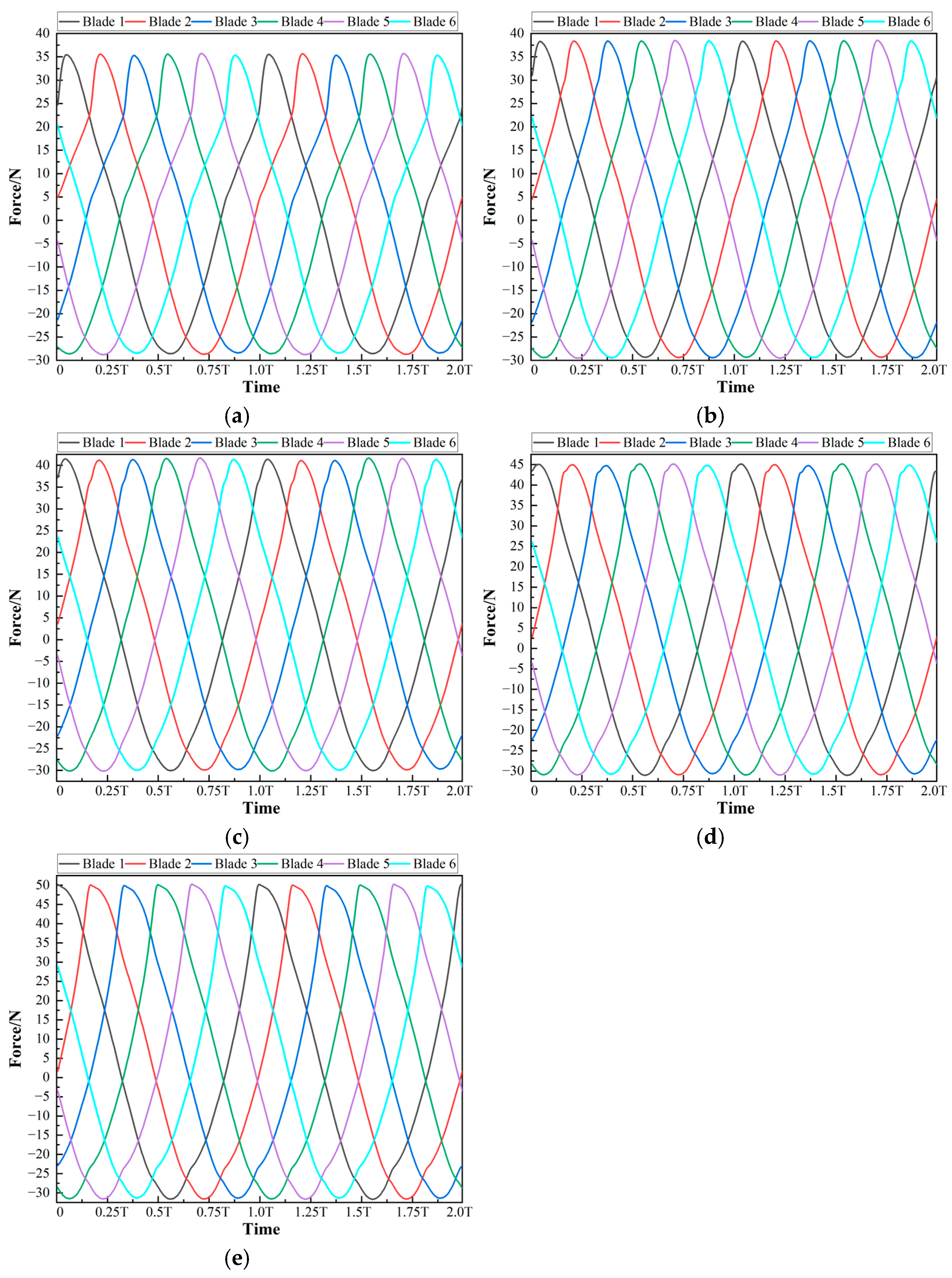
4.2. Hydraulic Radial Force on All Blades

The impeller of the research object in this study is an open impeller composed of six blades and a hub. By excluding the hub and only counting the hydraulic radial force acting on all the blades together, time varying curves are obtained, as shown in Figure 13a. Through a comparison with Figure 12, it can be found that the hydraulic radial force on all the blades and that on the entire impeller have almost the same variation curves. The hydraulic radial force on all the blades is divided by the that on the entire impeller to obtain the ratio of them, and the variation of this ratio is shown in Figure 13b. Figure 13b indicates that the ratio of them is concentrated between 1 and 1.2, which shows that the hydraulic radial force on all the blades is very close in magnitude to that acting on the entire impeller.

Furthermore, the angles of the hydraulic radial force on all the blades at each condition are calculated and plotted in Figure 14. Similarly, it can be found that Figure 14 and Figure 12 have a high degree of similarity. This shows that when studying the hydraulic radial force acting on the entire impeller, other parts of the impeller such as the hub can be ignored, and only the forces all the blades need to be considered. Doing so results in relatively small errors and brings great convenience to the subsequent research on the formation mechanism of the hydraulic radial force of the impeller.

The hydraulic radial force on all blades is also decomposed into components in the X and Y directions, as shown in Figure 15. Similarly, Figure 11 and Figure 15 also have a high degree of similarity, which further confirms that the hydraulic radial force on all blades can be used to approximately replace the that on the impeller.

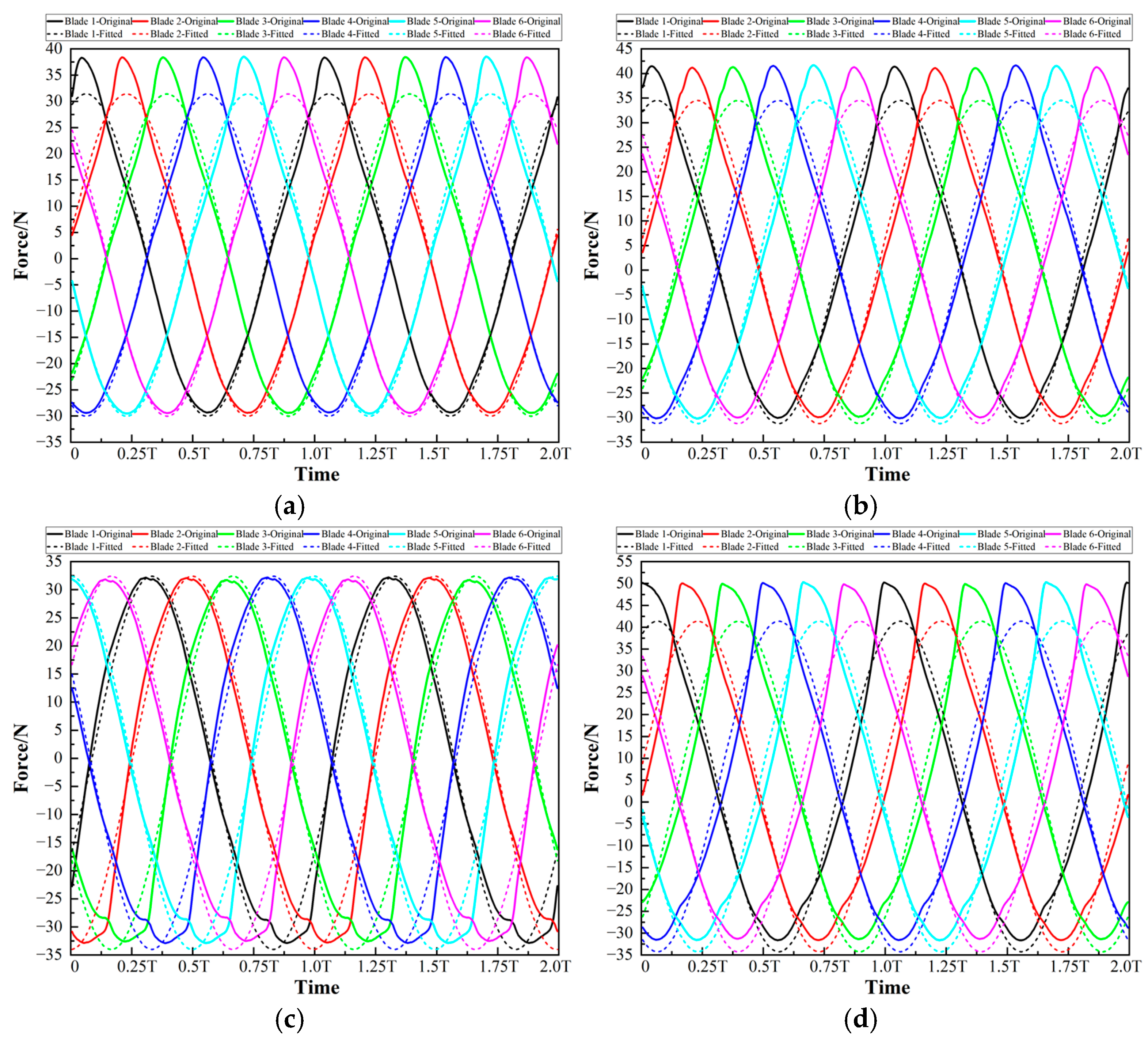
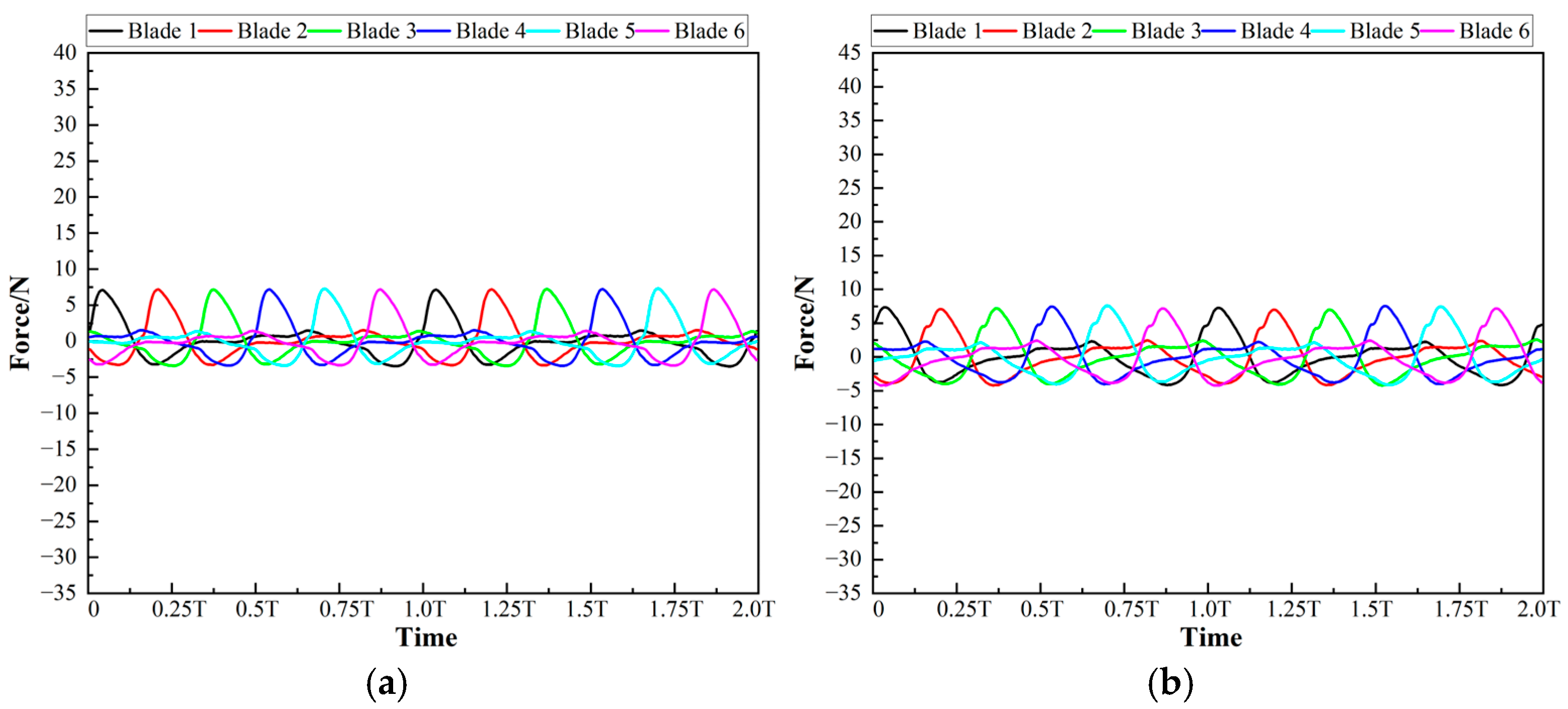
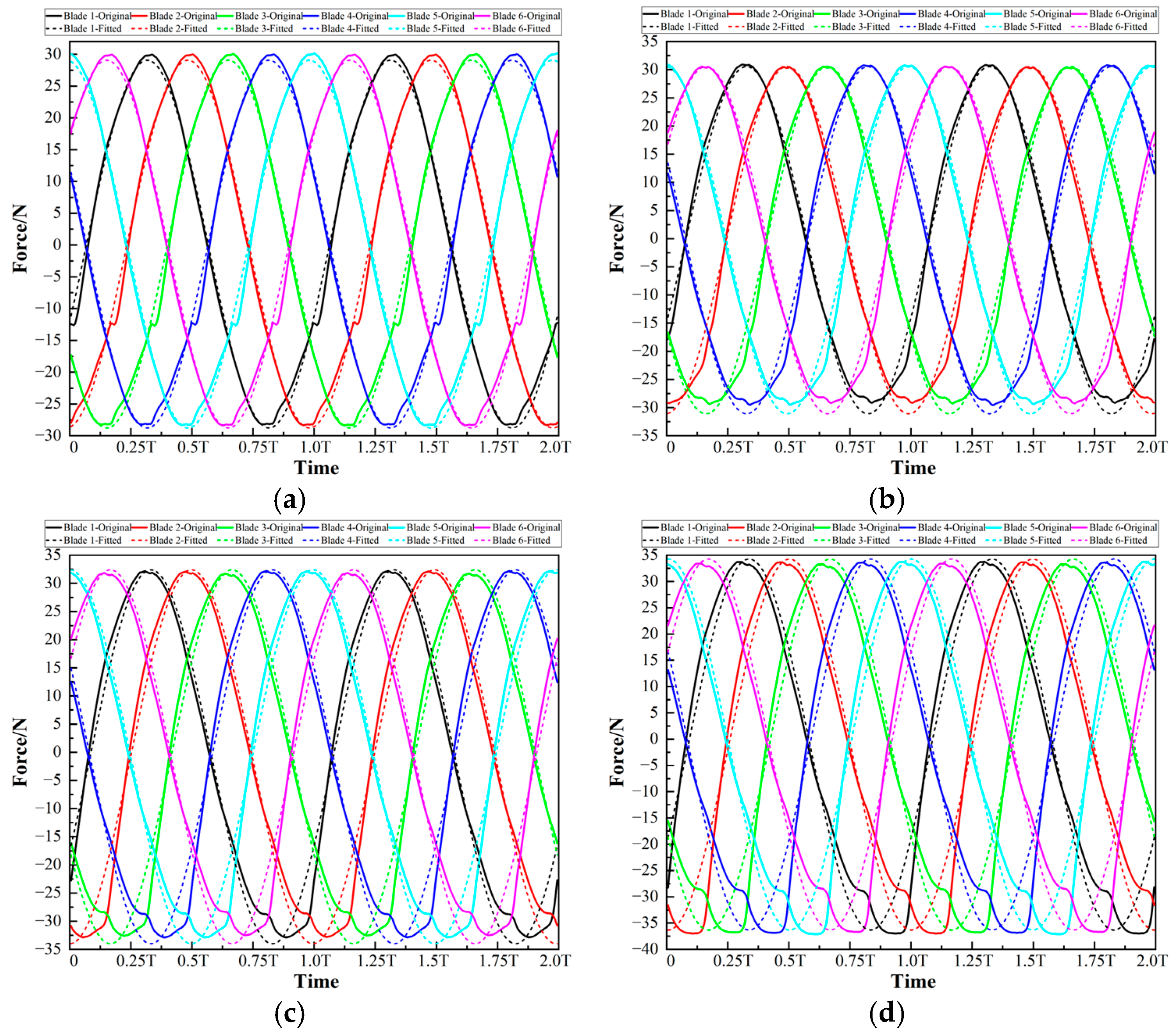
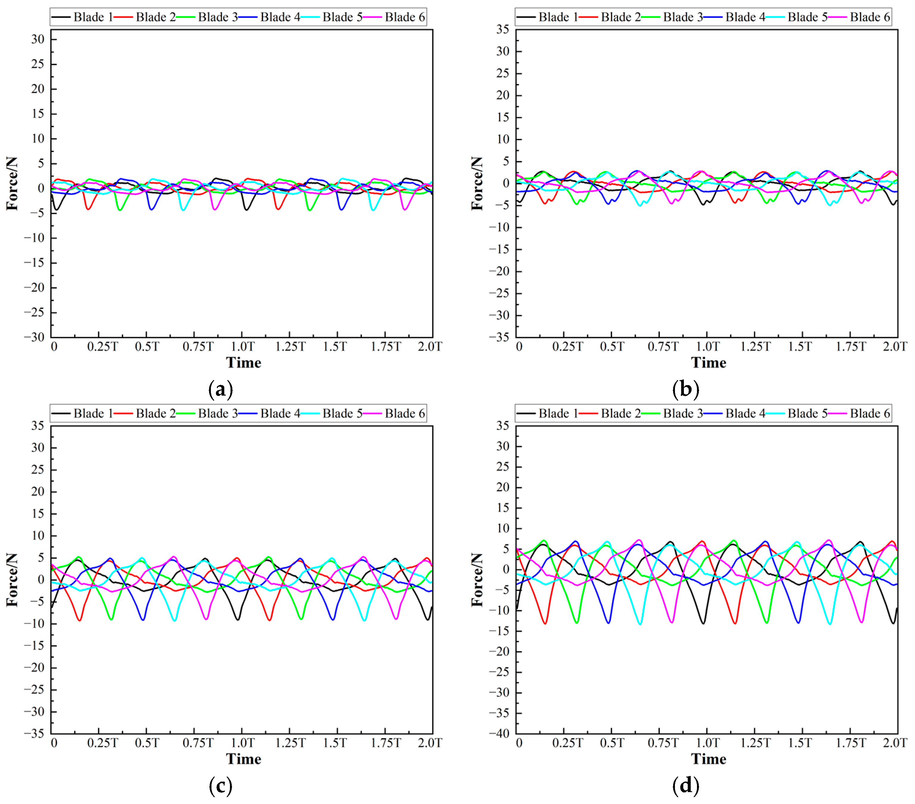
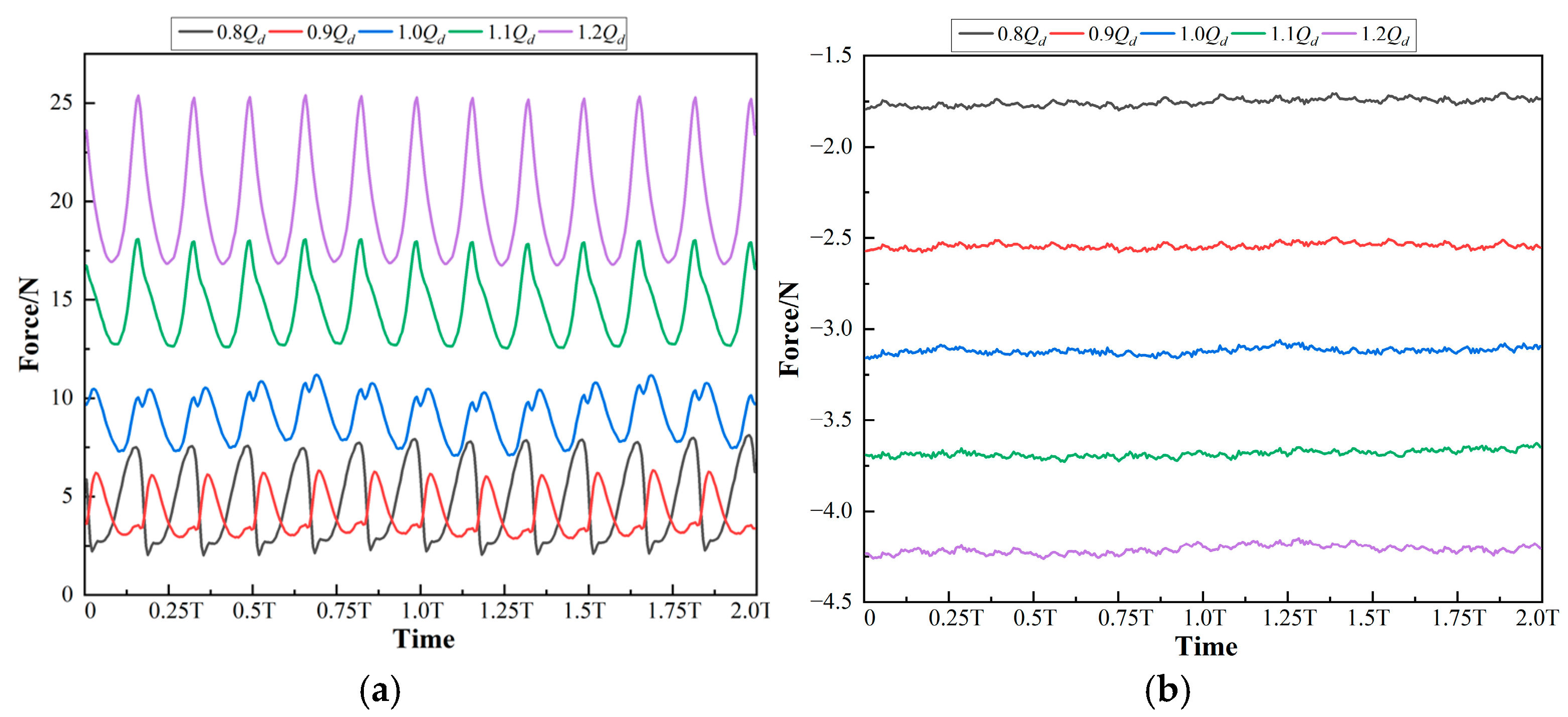
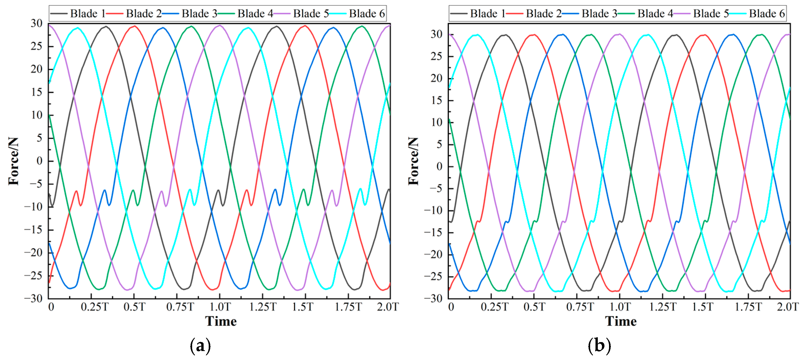
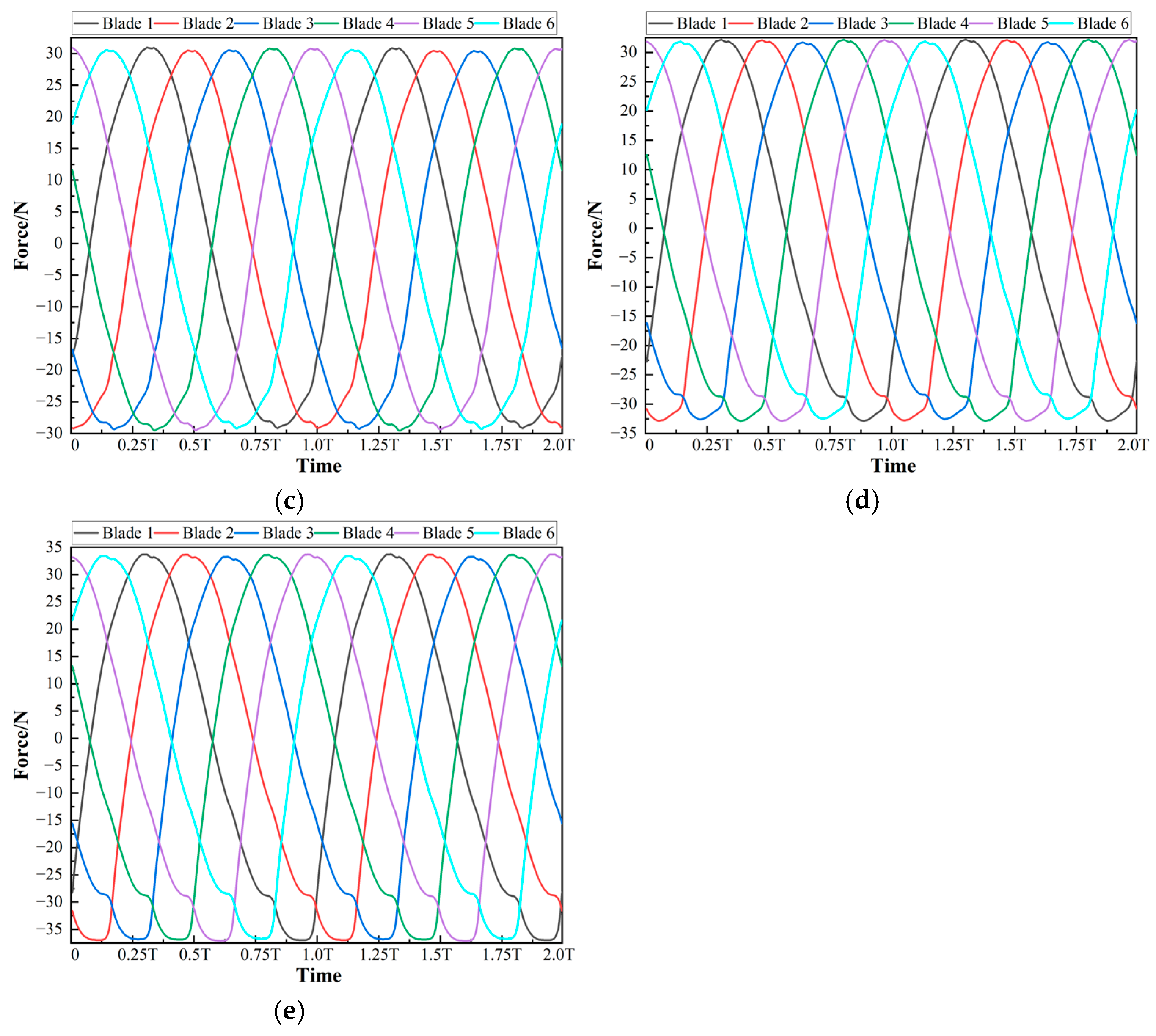
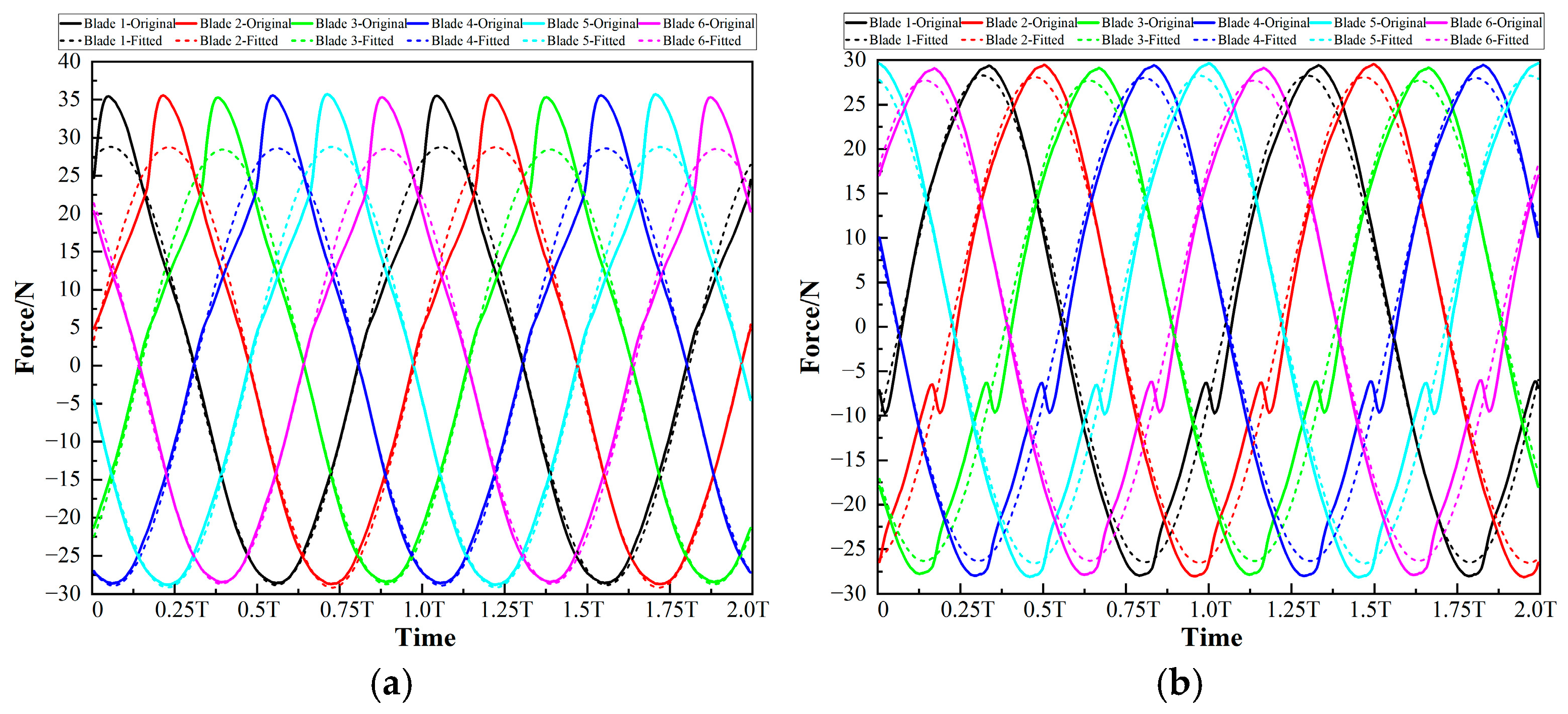
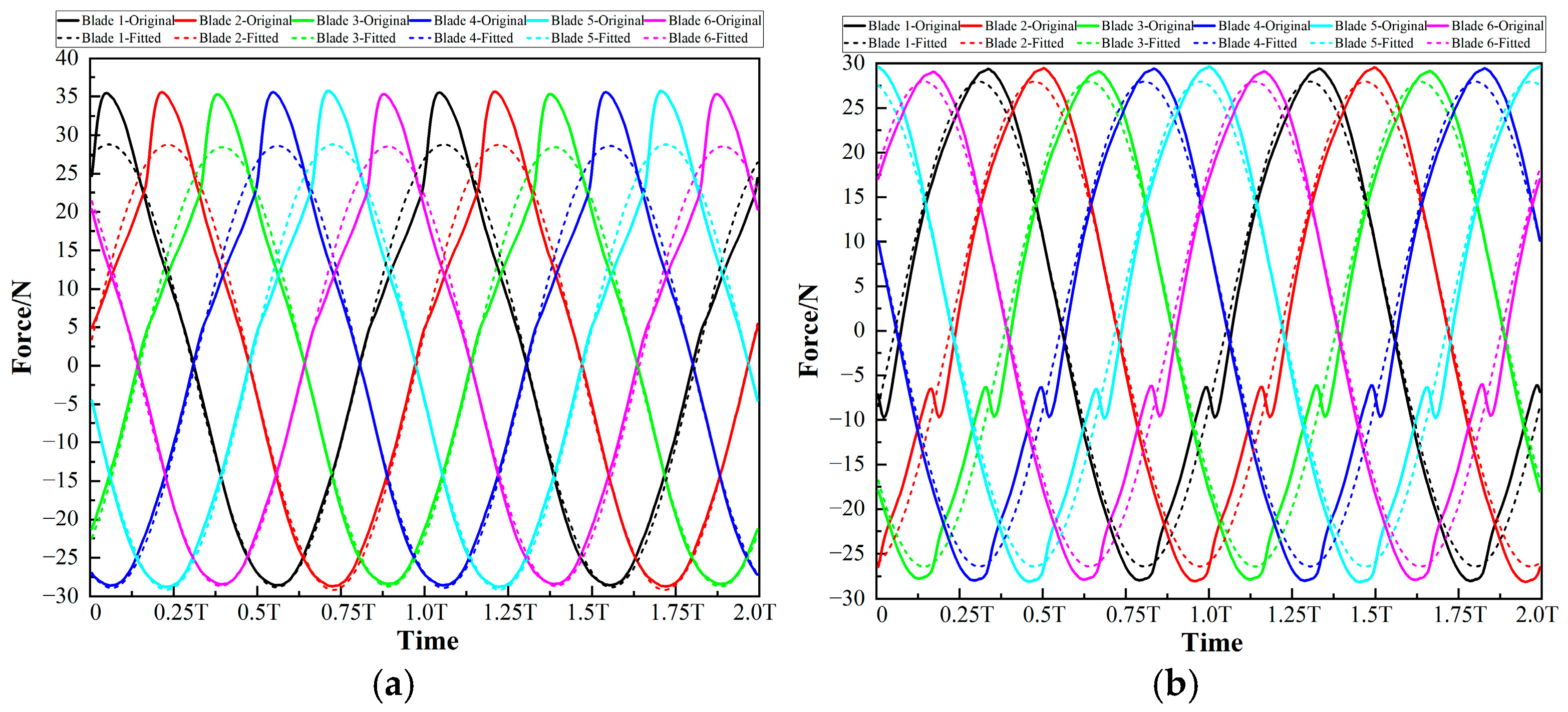
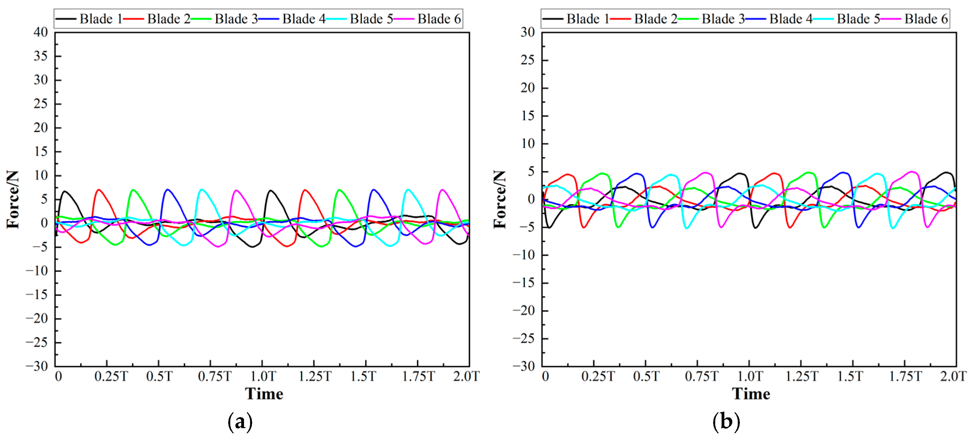
4.3. Hydraulic Radial Force on Each Blade

In this study, the centrifugal pump impeller has six blades that exhibit a cyclic symmetry relationship, which are named Blade 1 to Blade 6, respectively. The hydraulic radial force on all the blades together is regarded as the vector sum of that acting on each of these six blades. According to this concept, under different flow conditions, the curves of the components of the hydraulic radial force in the X and Y directions of Blade 1 to Blade 6 changing with time are plotted, as shown in Figure 16 and Figure 17.

As can be seen from Figure 16 and Figure 17, under each flow condition, the curves of the components of the hydraulic radial force in the X and Y directions of each blade changing with time form a curve cluster with exactly the same shape and size but with the same time interval. Each curve is very close to a sine curve, and the period is basically equal to the impeller rotation period T. Meanwhile, except for the local abrupt changes in the Y-direction components of the hydraulic radial force under the two low flow conditions of 0.8Q_d and 0.9Q_d, all the curves are relatively smooth.

In brief, by observing Figure 16 and Figure 17, it can be initially speculated that the curves of components of the hydraulic radial force on each blade in the X and Y directions changing with time are approximately a cluster of sine curves with equal amplitudes and frequencies but with initial phases that change successively at the same interval. To verify this hypothesis, taking the flow condition of 0.8Q_d as an example, the time varying curves of the hydraulic radial force on each blade in the X and Y directions are fitted according to the following formula:

f(t) = a × sin (ω × t + Φ) + b

(7)

where f reflects the hydraulic radial force component in X or Y direction, and t is time; a, ω, Φ, and b are the amplitude, angular frequency, initial phase, and constant terms in the trigonometric function expression, respectively.

The fitted trigonometric function curves are plotted as dashed lines in Figure 18. For the convenience of observation and comparison, the original curves are also plotted as solid lines. The fitting residuals, that is, the differences between the original values and the fitted values, are plotted in Figure 19. It is easy to see from Figure 18 and Figure 19 that for both the hydraulic radial force components in the X and Y directions, the original curves are very close to the sine function curves obtained by fitting, with only some differences at the peaks or troughs of each curve.

The fitting parameters are listed in

Table 3. Preliminary fitted parameters of hydraulic radial force components on each blade under 0.8Q_d.

Direction	Blade No.	a [N]	ω [rad/s]	Φ [rad]	b [N]	R2
X	1	28.799	301.705	1.215	−0.009	0.987
	2	28.956	305.445	0.090	−0.196	0.987
	3	28.577	304.349	−0.934	−0.132	0.986
	4	28.754	304.127	−1.976	−0.133	0.986
	5	28.952	303.642	−3.017	−0.167	0.986
	6	28.594	301.777	−4.024	−0.055	0.987
Y	1	27.373	307.990	−0.466	0.896	0.990
	2	27.311	303.867	−1.432	0.782	0.987
	3	27.022	302.914	−2.458	0.688	0.987
	4	27.168	301.636	−3.481	0.830	0.988
	5	27.420	303.051	−4.560	0.838	0.987
	6	27.016	303.994	−5.621	0.702	0.987

. As can be seen from the table, for each curve of the hydraulic radial force component, the goodness of fit, that is, the value of R², is not lower than 0.986. This indicates an extremely high fitting accuracy and a satisfactory fitting effect.

From the fitted values of each parameter, it can be found that for the same type of hydraulic radial force component, the amplitude a, the angular frequency ω, and the constant term b are all basically equal. Moreover, as the blade number increases, the initial phase Φ corresponding to each blade decreases successively at an interval of approximately 1.05 radians. When this decrement value of the initial phase is converted into degrees, it is approximately 60°, which precisely equals the included angle between adjacent blades. The above fitting based on Equation (7) is purely a preliminary attempt from a mathematical perspective to help discover possible physical laws. In fact, for time series data from the same curve, various fitting function expressions can be designed based on needs, as long as a sufficiently good fitting effect is achieved, ensuring a satisfied level of goodness of fit and keeping fitting residuals very low. According to the laws found in Table 3, continuing to focus on the sine function expression in Equation (7), the fitting method is improved in the following three aspects:

(1)

Cancel the fitting of the angular frequency ω, and fix its value as 2π/T, that is, set ω as the angular frequency corresponding to the impeller rotation, and its value is uniformly set as 303.687 rad/s.

(2)

Only fit the force curve of Blade 1 to obtain its corresponding amplitude a, constant term b, and initial phase Φ. While for the force curves of other blades, no fitting operation is carried out. Instead, directly use the fitting parameter results obtained from the force curve of Blade 1. Among them, for the amplitude a and constant term b corresponding to the force curves of other blades, directly use the fitting results of Blade 1, and the initial phase Φ decreases by 60° (approximately 1.047 radians) from that of Blade 1.

(3)

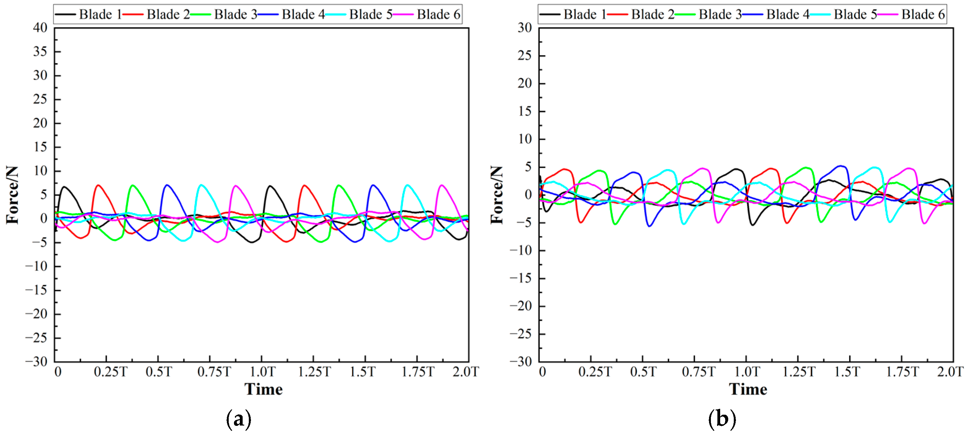
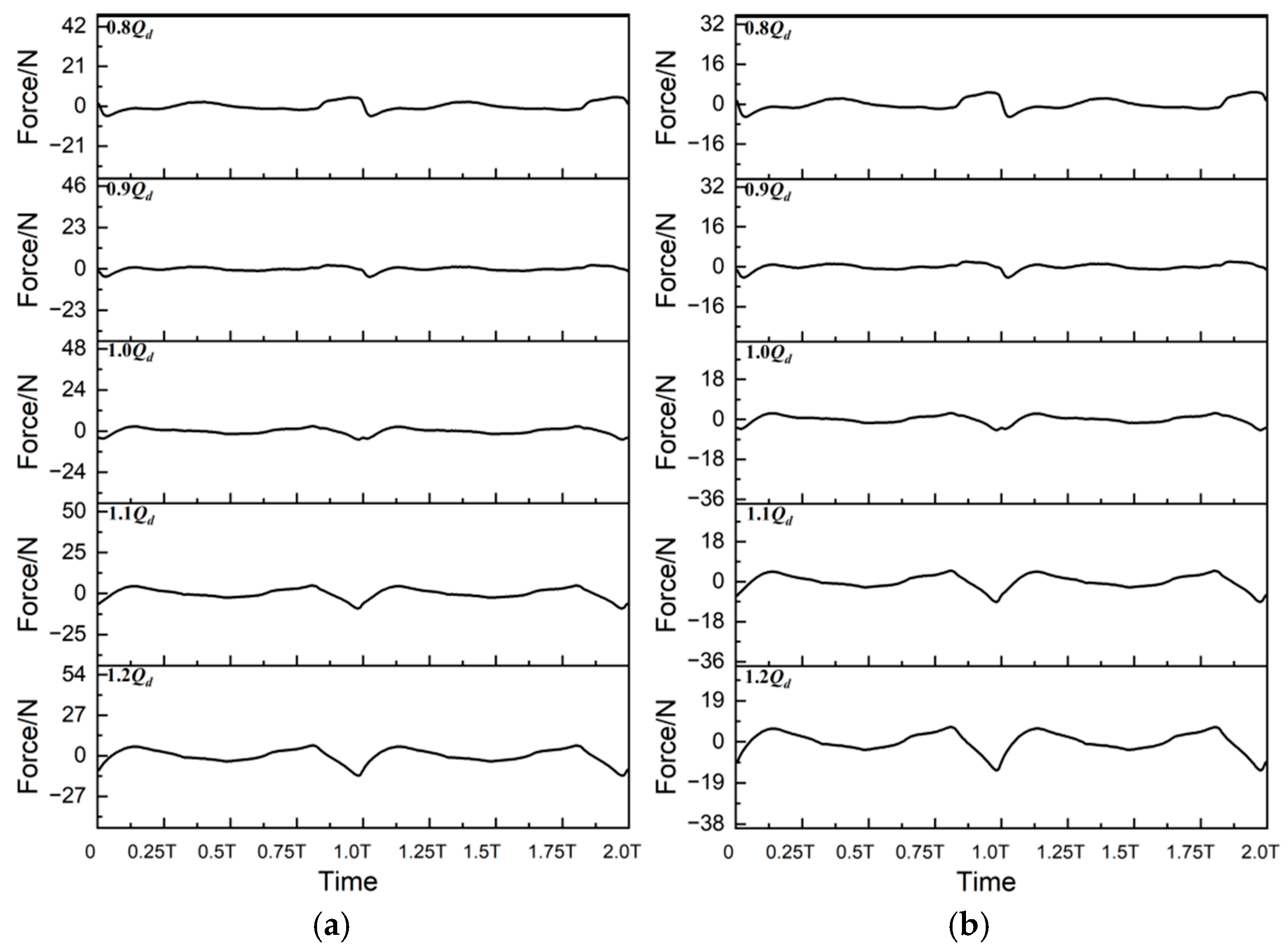
Although the fitting parameters of the force curves of Blade 2 to Blade 6 are derived from the fitting results of that of Blade 1, the reliability and accuracy of this method are still evaluated from the perspectives of the goodness of fit and fitting residuals.

Apply the above improved fitting method to all flow conditions. The fitting function curves and fitting residual curves under the 0.8Q_d condition are shown in Figure 20 and Figure 21, respectively, and the results under other conditions are shown in Figure A1, Figure A2, Figure A3 and Figure A4 in Appendix A. It can be found that all the obtained fitting function curves can perfectly fit the original curves within a large time range, which indicates that the improved fitting method is applicable to the fitting of the force curves of each blade under all flow conditions. Continuing to take the 0.8Q_d condition as an example, the fitting parameters are listed in

Table 4. Fitted parameters of hydraulic radial force components on each blade under 0.8Q_d.

Direction	Blade No.	a [N]	ω [rad/s]	Φ [rad]	b [N]	R2
X	1	28.722	303.687	1.172	−0.185	0.986
	2	28.722	303.687	0.125	−0.185	0.986
	3	28.722	303.687	−0.922	−0.185	0.986
	4	28.722	303.687	−1.969	−0.185	0.986
	5	28.722	303.687	−3.017	−0.185	0.986
	6	28.722	303.687	−4.064	−0.185	0.986
Y	1	27.187	303.687	−0.381	0.769	0.987
	2	27.187	303.687	−1.428	0.769	0.987
	3	27.187	303.687	−2.475	0.769	0.987
	4	27.187	303.687	−3.523	0.769	0.987
	5	27.187	303.687	−4.570	0.769	0.987
	6	27.187	303.687	−5.617	0.769	0.987

.

Table 4 shows the improved fitting method can also ensure that the goodness of fit value R² of each curve is not less than 0.986. By controlling the values of the same amplitude a, constant term b, and the successively decreasing initial phase Φ for the force curves of each blade corresponding to the same hydraulic radial force component under the same flow condition, it better helps researchers interpret the physical laws of the hydraulic radial force data. The parameter fitting values for the flow conditions from 0.9Q_d to 1.2Q_d are listed in

Table A1. Fitted parameters of radial hydraulic force components on each blade under 0.9Q_d.

Direction	Blade No.	a [N]	ω [rad/s]	Φ [rad]	b [N]	R2
X	1	30.719	303.687	1.172	0.698	0.989
	2	30.719	303.687	0.125	0.698	0.989
	3	30.719	303.687	−0.922	0.698	0.989
	4	30.719	303.687	−1.969	0.698	0.989
	5	30.719	303.687	−3.017	0.698	0.989
	6	30.719	303.687	−4.064	0.698	0.989
Y	1	28.922	303.687	−0.436	0.145	0.997
	2	28.922	303.687	−1.483	0.145	0.997
	3	28.922	303.687	−2.530	0.145	0.997
	4	28.922	303.687	−3.577	0.145	0.997
	5	28.922	303.687	−4.624	0.145	0.997
	6	28.922	303.687	−5.672	0.145	0.997

,

Table A2. Fitted parameters of radial hydraulic force components on each blade under 1.0Q_d.

Direction	Blade No.	a [N]	ω [rad/s]	Φ [rad]	b [N]	R2
X	1	32.852	303.687	1.161	1.651	0.986
	2	32.852	303.687	0.114	1.651	0.986
	3	32.852	303.687	−0.933	1.651	0.986
	4	32.852	303.687	−1.981	1.651	0.986
	5	32.852	303.687	−3.028	1.651	0.986
	6	32.852	303.687	−4.075	1.651	0.986
Y	1	30.831	303.687	−0.495	−0.267	0.993
	2	30.831	303.687	−1.542	−0.267	0.994
	3	30.831	303.687	−2.589	−0.267	0.994
	4	30.831	303.687	−3.637	−0.267	0.994
	5	30.831	303.687	−4.684	−0.267	0.994
	6	30.831	303.687	−5.731	−0.267	0.993

,

Table A3. Fitted parameters of radial hydraulic force components on each blade under 1.1Q_d.

Direction	Blade No.	a [N]	ω [rad/s]	Φ [rad]	b [N]	R2
X	1	35.392	303.687	1.162	2.587	0.980
	2	35.392	303.687	0.115	2.587	0.980
	3	35.392	303.687	−0.932	2.587	0.980
	4	35.392	303.687	−1.979	2.587	0.980
	5	35.392	303.687	−3.026	2.587	0.980
	6	35.392	303.687	−4.074	2.587	0.980
Y	1	33.207	303.687	−0.529	−0.795	0.982
	2	33.207	303.687	−1.576	−0.795	0.982
	3	33.207	303.687	−2.623	−0.795	0.982
	4	33.207	303.687	−3.670	−0.795	0.982
	5	33.207	303.687	−4.717	−0.795	0.983
	6	33.207	303.687	−5.765	−0.795	0.982

and

Table A4. Fitted parameters of radial hydraulic force components on each blade under 1.2Q_d.

Direction	Blade No.	a [N]	ω [rad/s]	Φ [rad]	b [N]	R2
X	1	37.809	303.687	1.152	3.557	0.972
	2	37.809	303.687	0.105	3.557	0.972
	3	37.809	303.687	−0.942	3.557	0.972
	4	37.809	303.687	−1.989	3.557	0.972
	5	37.809	303.687	−3.036	3.557	0.972
	6	37.809	303.687	−4.084	3.557	0.972
Y	1	35.301	303.687	−0.562	−1.025	0.968
	2	35.301	303.687	−1.609	−1.025	0.968
	3	35.301	303.687	−2.656	−1.025	0.968
	4	35.301	303.687	−3.704	−1.025	0.968
	5	35.301	303.687	−4.751	−1.025	0.968
	6	35.301	303.687	−5.798	−1.025	0.967

in Appendix A.

According to the fitting results above, it is evident that, within the research scope, regardless of the flow condition, the force curves of each blade for the same hydraulic radial force component can be grouped into a cluster of sine curves with identical amplitude, constant term, and angular frequency, achieving a goodness of fit of at least 0.96. The angular frequency in the fitting function is equal to the angular frequency of the impeller rotation. Moreover, there is a 60° phase difference in the initial phase of the sine functions in the same curve cluster in the order of blade rotation.

According to the induction formula of trigonometric functions, for any trigonometric function sin (α), sin (α + 2π)= sin (α) and sin (α + π) = − sin (α). Since there is a 60° initial phase difference between each blade for the same hydraulic radial force component under the same flow condition, the main part a × sin (ω × t + Φ) (after removing the constant term b) of the trigonometric force curve from Blade 1 can exactly cancel out the main part a × sin (ω × t + Φ − π) of that from Blade 4. Similarly, the main parts of the fitting functions of Blade 2 and Blade 5, as well as those from Blade 3 and Blade 6, can also cancel each other out. That is, with the impeller center as the symmetric point, the main parts of the fitting functions of two blades that are centrally symmetric to each other can completely cancel each other out. Therefore, the force curve of each blade in the impeller can be regarded as the superposition of the fitting curve and the residual curve. The main parts of the fitting curves can cancel each other out, leaving only the same constant term b. Finally, the force curve from the superposition of all blades is actually the sum of the residual curves of each blade and 6 times the constant term b.

With the above findings, the time varying characteristics of the hydraulic radial force in Figure 11 can be well explained. Taking the hydraulic radial force of the impeller in the X-direction under the 0.8Q_d flow condition as an example, as shown in Figure 11a, its time varying curve has 6 fluctuation waves within a single cycle, with the peak and trough values approximately −3.5 N and 2.6 N, respectively. Thus, its peak-to-peak value is about 6.1 N. That force curve can be approximately regarded as the superposition of the force components of the 6 blades of the impeller. The original curves and fitting curves of these 6 blade force components are shown by the solid and dashed lines in Figure 20a, respectively, and the fitting parameter results are listed in Table 4. Despite the peak-to-peak value of the fitting function curve, i.e., 2a, is as high as 57.444 N, over 9 times that of the impeller’s hydraulic radial force, the main parts of the fitting functions for two centrally symmetric blades cancel each other out. Therefore, the impeller’s hydraulic radial force curve in the X direction is primarily determined by the fitting residual curves of each blade shown in Figure 21a and the constant term’s fitting value. It can be found in Figure 21a that the fitting residual curves of each blade show a prominent fluctuation within one impeller rotation cycle, and in the direction of impeller rotation, the fluctuation interval between adjacent blades is exactly equal to T/6. By superimposing the fitting residual curves of each blade in Figure 21a and then adding 6 times the fitting value of the constant term b, the original hydraulic radial force curve of the impeller in the X direction under the 0.8Q_d in Figure 11a can be basically restored.

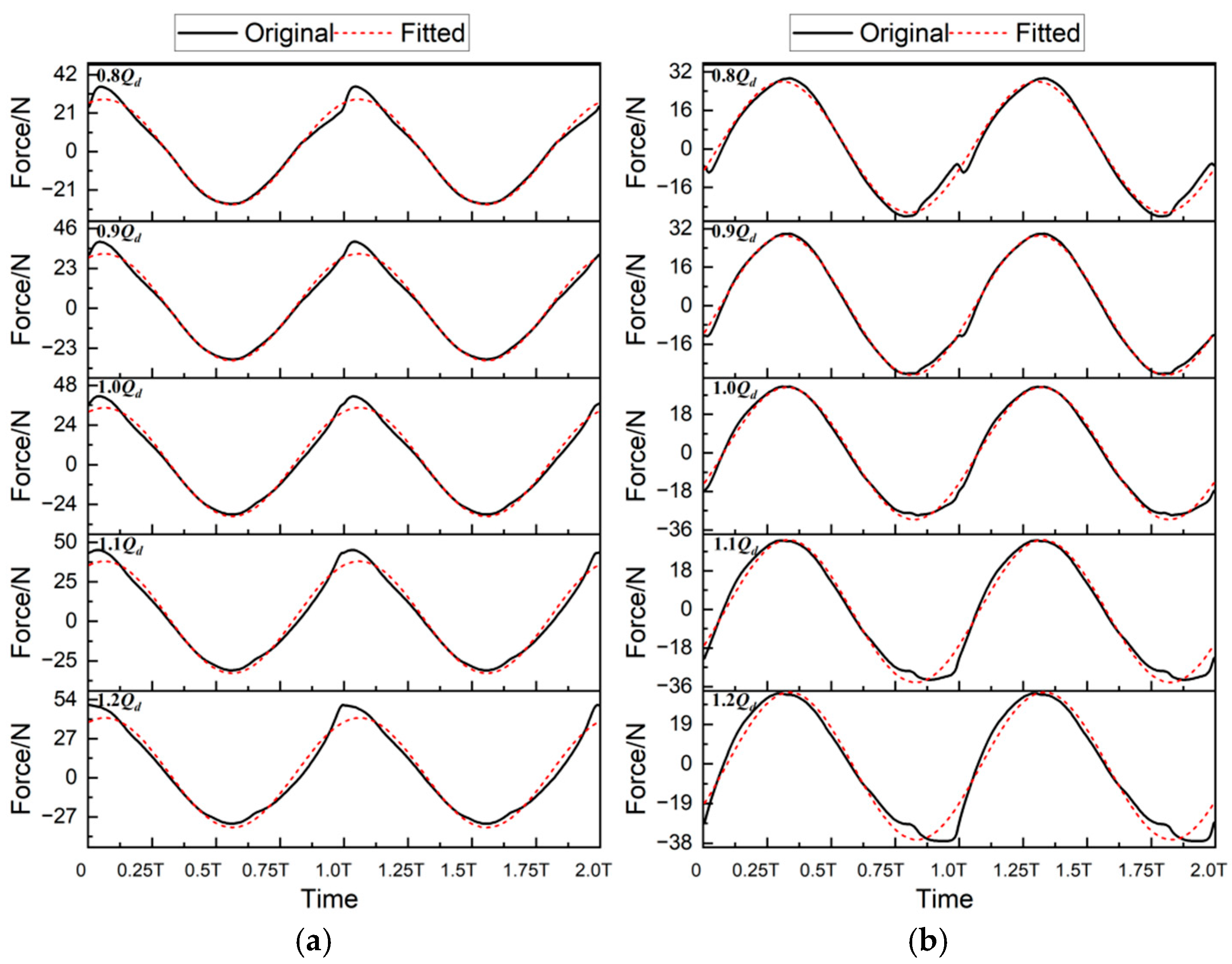
4.4. Hydraulic Radial Force on Blade 1

Based on the findings in Section 4.3, under a certain flow condition, the curves of the hydraulic radial forces acting on each blade have identical waveforms in terms of size and shape, but there are certain time differences in the fluctuation sequence. The time difference between the force waveforms of adjacent blades is T/6. Therefore, if the time varying curve of the hydraulic radial force of any one blade is obtained, then curves of all other blades can be derived through time translation.

Taking Blade 1 as the research object, the curves of the hydraulic radial force components in the X and Y directions under various flow conditions are plotted as solid lines in Figure 22a,b, respectively. The fitting function curves are also plotted as dashed lines in Figure 22, and the fitting residual curves are shown in Figure 23. The corresponding fitting parameters are listed in

Table 5. Fitted parameters of hydraulic radial force components on Blade 1 under different flow conditions.

Direction	Flow Condition	a [N]	ω [rad/s]	Φ [rad]	b [N]	R2
X	0.8Qd	28.722	303.687	1.172	−0.185	0.986
	0.9Qd	30.719	303.687	1.172	0.698	0.989
	1.0Qd	32.852	303.687	1.161	1.651	0.986
	1.1Qd	35.392	303.687	1.162	2.587	0.980
	1.2Qd	37.809	303.687	1.152	3.557	0.972
Y	0.8Qd	27.187	303.687	−0.381	0.769	0.987
	0.9Qd	28.922	303.687	−0.436	0.145	0.997
	1.0Qd	30.831	303.687	−0.495	−0.267	0.993
	1.1Qd	33.207	303.687	−0.529	−0.795	0.982
	1.2Qd	35.301	303.687	−0.562	−1.025	0.968

.

As can be observed from Figure 22, generally, the time varying curves of the two force components in the X and Y directions under each flow condition are very close to sine curves. The time varying curves of the same hydraulic radial force component have high similarities in terms of waveform shape and phase, and the amplitude increases continuously as the flow rate increases. This finding can be quantitatively verified by the fitting parameter results in Table 5. Taking the curve of the hydraulic radial force component in the X direction as an example, the amplitude a obtained through sine function fitting has a fitted value of 28.722 N under the 0.8Q_d. As the flow rate gradually increases to 1.2Q_d, the fitted value also increases to 37.809 N. Meanwhile, the fitting results of the initial phase under each flow condition are relatively close, with a radian value of approximately 1.16. In addition, although the fitted value of the constant term b changes with the flow rate, its magnitude and fluctuation level are basically negligible compared with the amplitude a and the fitting residual value.

The above phenomena can be explained from the perspective of unsteady flow inside the centrifugal pump. When the time is near an integer multiple of the impeller rotation period T, it corresponds to the moment when Blade 1 sweeps past the volute tongue. During the operation of pump, there is a strong interaction between the impeller and the volute tongue, which triggers a series of prominent unsteady flow phenomena, leading to significant changes in the hydraulic radial force on the impeller. According to the research of Zhang et al. [43], when the impeller blade sweeps past the volute tongue, the jet-wake flow pattern at the impeller outlet interacts with the volute tongue. A high-speed jet region is formed on the pressure side of the blade, and a low-speed wake region appears on the suction side. This makes the pressure distribution in the flow field near the volute tongue extremely non-uniform, generating a significant radial force. Meanwhile, there are complex vortex structures inside the centrifugal pump. When the impeller blade approaches the volute tongue, a high vortex region is formed at the blade trailing edge. The interaction between the vortices in this region and the volute tongue changes the local flow field pressure distribution. The generation, development, and shedding of these vortices cause pressure fluctuations, resulting in significant fluctuations in the radial force on the impeller. In addition, when the impeller blade sweeps past the volute tongue, flow passage blockage may occur. As the impeller passes the volute tongue, the flow passage area near the volute tongue decreases, causing fluid flow obstruction and uneven flow distribution, which leads to pressure pulsation and generates a large radial force.

In the meantime, Zhu et al. [44] summarized the above flow behaviors as the clocking effect. During the rotation of the impeller, different blades successively sweep past the volute tongue, corresponding to different relative angular positions. When a blade sweeps past the volute tongue, the change in their relative position leads to a change in the flow field, which is specifically manifested as changes in the jet-wake flow pattern, vortex structure, etc. When the relative position between the impeller blade and the volute tongue is at certain specific angles, the non-uniformity of the flow is intensified, resulting in a more non-uniform pressure distribution near the volute tongue, and further causing a significant increase in the hydraulic radial force on the impeller when the blade sweeps past the volute tongue.

4.5. CFD Results

To further elucidate the relationship between the hydraulic radial force and the circumferential pressure asymmetry on the impeller, the mid-plane pressure distributions under five flow conditions (0.8Q_d to 1.2Q_d) are analyzed, as shown in Figure 24. These pressure contours provide direct insights into the spatial non-uniformity of the flow field, which is the primary driver of hydraulic radial force generation.

The following observations are drawn from Figure 24:

(1)

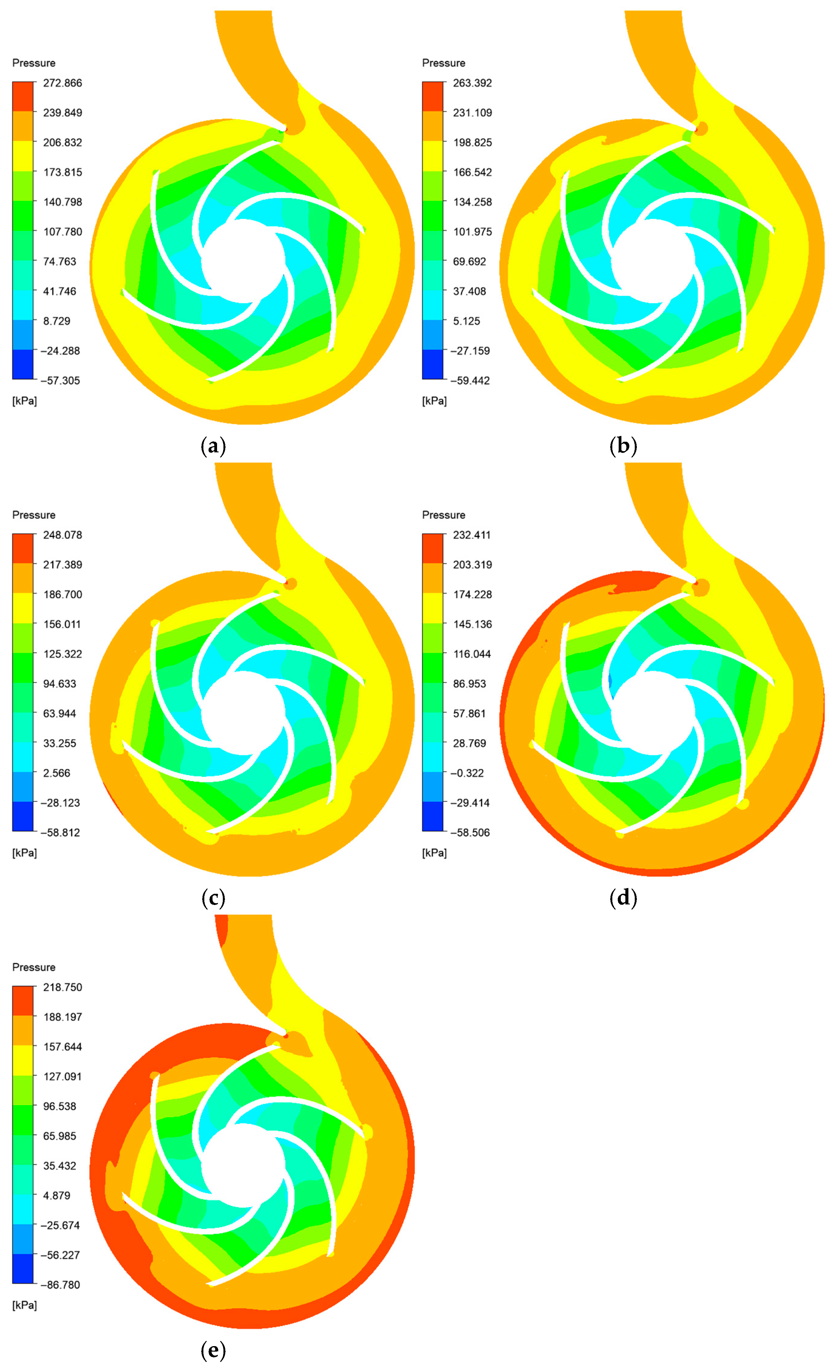
Pressure Trend with Flow Rate: As the flow rate increases from 0.8Q_d to 1.2Q_d, the overall static pressure magnitude within the impeller and volute exhibits a gradual decrease. This aligns with the pump’s characteristic performance curve (see Figure 6), where the head declines with increasing flow rate due to the combined effects of hydraulic losses (e.g., friction and turbulence) and reduced energy conversion efficiency in the impeller-volute interaction.

(2)

Pressure Uniformity at Rated Flow: Around the rated flow condition (i.e., 1.0 Q_d), the pressure distribution demonstrates optimal circumferential symmetry. The interaction between the impeller blades and the volute tongue is minimized, leading to balanced pressure gradients around the impeller periphery. This aligns with the earlier findings in Section 4.1, Section 4.2, Section 4.3 and Section 4.4, where the hydraulic radial force around 1.0Q_d exhibited minimal fluctuations and a near-constant angle.

(3)

Increased Non-Uniformity at Off-Design Conditions: When the flow deviates from the rated point, the pressure asymmetry intensifies. However, distinct pressure distribution characteristics are observed between high-flow (e.g., 1.2Q_d) and low-flow (e.g., 0.8Q_d) conditions. Specifically, under the 1.2Q_d condition, the pressure non-uniformity becomes significantly more pronounced compared to the 0.8Q_d case. This discrepancy can be partially attributed to the amplified hydraulic radial forces on the impeller at higher flow rates, as illustrated in Figure 8a, where the intensified circumferential pressure gradients directly correlate with the elevated force magnitudes.

While the CFD-derived pressure contours qualitatively illustrate the flow non-uniformity, they lack the temporal resolution to quantitatively evaluate the dynamic evolution of the hydraulic radial force. This limitation underscores the significance of the data-centric approach adopted in this study. By leveraging high-fidelity CFD datasets, the time-resolved hydraulic radial forces are systematically decomposed, revealing periodic patterns and harmonic cancellations between symmetric blades (Section 4.3). Trigonometric fitting and FFT analysis further quantified the amplitude-phase relationships, enabling a deeper understanding of the force composition. Such insights are unattainable through conventional flow field visualization alone.

To advance the suppression of hydraulic radial forces, future work should integrate advanced data mining techniques (e.g., proper orthogonal decomposition or machine learning) with mechanistic interpretations of CFD-predicted flow structures. For example, correlating residual force components (Figure 21) with transient vorticity fields could identify specific flow features responsible for residual pulsations. Additionally, multi-fidelity datasets spanning diverse impeller geometries and operating regimes will enhance the generalizability of the proposed framework.

In summary, this section bridges the gap between qualitative flow field analysis and quantitative force characterization, reinforcing the necessity of combining CFD simulations with data-driven methodologies for optimizing centrifugal pump stability.

5. Composition Law and Application Enlightenment

5.1. Composition Law of Hydraulic Radial Force on Impeller

In this study, based on the principles of force translation and decomposition, the hydraulic radial force acting on the entire impeller is decomposed into the vector sum of the hydraulic radial forces acting on each component of the impeller. Moreover, the force component can be further decomposed into two mutually orthogonal components in the X and Y directions. According to the above analysis, the following four composition laws of the hydraulic radial force on impeller can be summarized:

(1)

The hydraulic radial force on the entire impeller can be decomposed into two parts: the force on all the blades and that on the other parts except the blades. It is found that the hydraulic radial force on the blades accounts for the vast majority of that on the entire impeller.

(2)

The curves of the hydraulic radial forces are all periodic curves, and the period is equal to the impeller rotation period T.

(3)

Arbitrarily select a blade as the reference blade, and tits next blade in the rotation direction is the adjacent blade. The curve of the hydraulic radial force on the adjacent blade changing with time lags behind the curve of the reference blade by exactly T/N in time. That is, if the curve of the adjacent blade changing with time is translated by T/N in the direction of decreasing on the time axis, it can completely coincide with that of the reference blade. Here, N is the total number of blades.

(4)

The curves of the components of the hydraulic radial forces on each blade can all be fitted into sine function curves with a high goodness of fit. Specifically, the angular frequencies obtained by fitting each sine function are all equal to the angular frequency of the impeller rotation. Under the same flow condition, the amplitudes and constant terms obtained by fitting each sine function are equal. The initial phases of the sine functions corresponding to each blade decrease successively by 2π/N in the order of blade rotation. That is, if a blade is arbitrarily selected as the reference blade, then the initial phase of the sine function of its adjacent blade in the rotation direction lags behind to it by 2π/N.

5.2. Application Enlightenment

During the design optimization process of the impeller hydraulic model, the data of the impeller’s hydraulic radial force can be processed and analyzed based on the inspiration from the above-mentioned laws. For the convenience of description, one blade on the impeller is arbitrarily selected as the reference blade and numbered as 1, and the remaining blades are numbered from 2 to N successively in the rotation direction of the impeller. Meanwhile, the two mutually orthogonal radial directions of the impeller are denoted as the X and Y directions, respectively. The internal flow field of the pump is obtained through unsteady CFD simulation, and the time varying information of the hydraulic radial forces on each blade are recorded. Then the data analysis and processing are carried out according to the following steps:

Firstly, the hydraulic radial force on the entire impeller is approximately regarded as the vector sum of that on all the blades. By orthogonally decomposing the hydraulic radial force, the forces in the two radial directions can be respectively decomposed and expressed as ${\sum }_{\mathrm{i}=1}^{\mathrm{N}}{F}_{\mathrm{i}\mathrm{X}}$ and ${\sum }_{\mathrm{i}=1}^{\mathrm{N}}{F}_{\mathrm{i}\mathrm{Y}}$, where F_iX and F_iY are the hydraulic forces on the blade numbered i in the X and Y directions, respectively.

Secondly, it is only necessary to perform trigonometric function fitting on the time-varying data of the forces on Blade 1 in the X and Y directions based on the least squares method, and orthogonally decompose its force data over time into F_1X(t) and F_1Y(t):

F_1X(t) = a_1X × sin (2π × t/T + Φ_1X) + b_1X + S_1X(t)

(8)

F_1Y(t) = a_1Y × sin (2π × t/T + Φ_1Y) + b_1Y + S_1Y(t)

(9)

where a_1X, b_1X and Φ_1X are the amplitude, constant term, and initial phase obtained by fitting the force curve in the X direction, respectively; a_1Y, b_1Y and Φ_1Y are the amplitude, constant term, and initial phase obtained by fitting the force curve in the Y direction, respectively; S_1X(t) and S_1Y(t) represent the fitting residuals of the force curves in the X and Y directions, respectively; t is the time, and T is the impeller rotation period.

In other words, the hydraulic force curve on Blade 1 in a certain direction can be regarded as the superposition of a trigonometric function curve with a clear analytical expression and a residual curve without a clear analytical expression.

Thirdly, for other blades, it is only necessary to perform time translation based on the two decomposition expressions corresponding to Blade 1 in Equations (8) and (9). For the blade numbered i, the liquid pressures acting on it in the X and Y directions are respectively expressed as F_iX(t) and F_iY(t):

F_iX(t) = a_1X × sin (2π × t/T + Φ_1X − 2π(i − 1)/N) + b_1X + S_1X[t − T(i − 1)/N]

(10)

F_iY(t) = a_1Y × sin (2π × t/T + Φ_1Y − 2π(i − 1)/N) + b_1Y + S_1Y[t − T(i − 1)/N]

(11)

Regarding S_1X(t) and S_1Y(t) as periodic original signals with a period of T, S_1X[t − T(i − 1)/N] and S_1Y[t − T(i − 1)/N] respectively represent the signals obtained by moving the original signals S_1X(t) and S_1Y(t) along the increasing direction of the time axis t by a time interval of T(i − 1)/N.

In other words, the force component curve on the blade numbered i can also be regarded as the superposition of a trigonometric function curve and a residual curve. The initial phase in the fitting result lags behind that of Blade 1 by 2π(i − 1)/N, and the residual curve lags behind a time interval of T(i − 1)/N.

Finally, based on the above decomposition representation method, the composition characteristics of the impeller’s hydraulic radial force can be understood more deeply, and the blade structure can be optimized in a more targeted manner to achieve the reduction of hydraulic radial force. Generally, the blades of impeller are of periodic centrosymmetric design and even number. Then, for any blade, there must be another blade that is centrally symmetric to it. According to the expressions of the force components on these two blades, it can be found that the main parts (excluding the constant terms) of the trigonometric function curves can exactly cancel each other out, leaving only the constant terms. Therefore, in the optimization design process, there is no need to pay attention to the magnitude of the amplitude of the fitted trigonometric function, but only to the constant term part and the residual curve.

5.3. Research Innovation

This study introduces a data-centric harmonic decomposition framework to analyze hydraulic radial forces on centrifugal pump impellers, advancing beyond traditional holistic CFD models. By integrating high-fidelity CFD datasets with trigonometric fitting, the research reveals that the radial force on a six-blade impeller can be decomposed into periodic components from individual blades, each characterized by identical amplitudes/frequencies but successive 60° phase shifts corresponding to blade spacing (Figure 16 and Figure 17). Unlike prior works [23,24,40] that treat the impeller as an undivided entity, this study demonstrates that centrally symmetric blades (e.g., Blade 1 and Blade 4) cancel out primary harmonic forces (e.g., blade passing frequency components), leaving only constant terms and residual fluctuations. This mechanism highlights the critical role of blade symmetry in suppressing unsteady flow-induced pulsations, a phenomenon not explicitly quantified in conventional CFD-based optimization approaches [25,26,27].

The innovation lies in linking localized blade-wise pressure dynamics to global force characteristics through data-driven decomposition. This approach contrasts with traditional trial-and-error methods (e.g., volute shape modifications [26]) by offering a quantifiable framework to predict force behavior through data analysis. By validating this with CFD and experimental data (Section 2.5), the research establishes a robust methodology for centrifugal pump design, with potential extensions to other turbomachinery requiring vibration control. Recent studies [45,46] have similarly emphasized the efficacy of CFD-machine learning integration for pump optimization, but this work uniquely focuses on harmonic decomposition to decode force mechanisms. Additionally, literature on blade number effects [47] and fluid–structure interaction contextualizes the symmetry-driven cancellation phenomenon observed here.

However, this methodology has certain limitations that warrant attention. First, the current framework relies on Reynolds-Averaged Navier-Stokes (RANS) simulations with the SST k-ω turbulence model, which may underresolve fine-scale turbulent structures (e.g., small-scale vortices near blade tips). Future work could incorporate large-eddy simulation (LES) to capture unsteady flow features with higher fidelity, particularly in extreme flow conditions like severe cavitation or stall. Second, the study focuses on a six-blade symmetric impeller, and its applicability to asymmetric blade configurations (e.g., odd-numbered blades) remains untested. Extending the harmonic decomposition to such systems would require modifying the phase-shift analysis to account for non-uniform blade spacing. Third, this study represents a theoretical preliminary exploration of force decomposition, and the proposed methodology has not yet been applied to practical impeller optimization design. While the data-driven framework offers a promising basis for reducing radial forces, its effectiveness in real-world applications—such as guiding blade geometry modifications—requires validation through targeted optimization case studies. Future research should apply the harmonic decomposition method to specific impeller designs, quantify the reduction in radial force and vibration levels, and evaluate its engineering utility through prototyping and experimental testing. This step is critical to bridging the gap between theoretical insights and industrial implementation.

6. Conclusions

This study systematically analyzed the composition mechanism and variation characteristics of the hydraulic radial force on the impeller of a centrifugal pump using a data-centric approach based on CFD datasets. The research aimed to provide theoretical guidance for suppressing the hydraulic radial force and improving the operational stability of centrifugal pumps. Below are the key findings and highlights:

(1)

Periodic Behavior and Dominant Frequency: The hydraulic radial force exhibited periodic behavior with a dominant frequency corresponding to the blade passing frequency (BPF). This finding aligns with previous studies and confirms the significance of BPF in unsteady flow phenomena.

(2)

Force Decomposition and Symmetry: The hydraulic radial force on the impeller could be decomposed into the contributions from each blade, with the main parts of the fitting functions of centrally symmetric blades canceling each other out. This left only the constant terms and fitting residuals, which determined the overall force curve. This discovery offers a deeper understanding of the force composition and provides a foundation for targeted blade optimization.

(3)

Flow Condition Impact: The study demonstrated that the hydraulic radial force varied significantly with flow conditions. At the rated flow rate, the force components showed minimal fluctuations, while deviations from the rated flow rate led to increased fluctuations. This insight is crucial for designing pumps that operate efficiently across a range of flow conditions.

(4)

Data-Driven Insights: The application of FFT and trigonometric function fitting revealed detailed frequency characteristics and potential variation patterns in the hydraulic radial force. This data-driven approach enhances the ability to predict and mitigate unsteady flow phenomena, offering a robust framework for future research.

(5)

Optimization Implications: The findings suggest that focusing on the constant terms and fitting residuals in the force components can lead to more effective optimization of blade structures. This targeted approach can significantly help to reduce the hydraulic radial force and improve the operational stability and efficiency of centrifugal pumps.

References

1. Yuan, Z.Y.; Zhang, Y.X.; Zhou, W.B.; Zhang, J.Y.; Zhu, J.J. Optimization of a centrifugal pump with high efficiency and low noise based on fast prediction method and vortex control. Energy 2024, 289, 129835. [Google Scholar] [CrossRef]
2. Han, R.; Zhang, X.; Ge, R.; Geng, H.; Xu, H.; Lin, H.; Jiang, Y.; Zhang, J.; Sang, M.; Zhao, T.; et al. Design, construction and testing of the prototype cryogenic circulation centrifugal pump for the high energy photon source. Cryogenics 2024, 142, 103900. [Google Scholar] [CrossRef]
3. Cui, B.; Shi, M. Analysis of unsteady flow characteristics near the cutwater by cutting impeller hub in a high-speed centrifugal pump. J. Mar. Sci. Eng. 2024, 12, 587. [Google Scholar] [CrossRef]
4. Long, Y.; Xu, Y.; Zhou, Z.; Wang, R.; Zhu, R.S.; Fu, Q. Study on cavitation flow and high-speed vortex interference mechanism of high-speed inducer centrifugal pump based on full flow channel. J. Braz. Soc. Mech. Sci. Eng. 2024, 46, 683. [Google Scholar] [CrossRef]
5. Jang, H.; Suh, J. Flow characteristic analysis of the impeller inlet diameter in a double-suction pump. Energies 2024, 17, 1989. [Google Scholar] [CrossRef]
6. Zhang, F.; Chen, Z.M.; Han, S.Q.; Zhu, B.S. Study on the unsteady flow characteristics of a pump turbine in pump mode. Processes 2024, 12, 41. [Google Scholar] [CrossRef]
7. Yuan, Y.; Junejo, A.R.; Wang, J.; Chen, B. Unsteady flow behaviors and vortex dynamic characteristics of a marine centrifugal pump under the swing motion. Machines 2024, 12, 687. [Google Scholar] [CrossRef]
8. Sun, C.; Dai, Y.X.; Cai, Y.L.; Wang, Z.L.; Zhang, H. Numerical investigation of the effect of the non-uniform intake flow on the unsteady flow and the excitation of the pump in a water-jet propulsion. J. Phys. Conf. Ser. 2024, 2854, 012051. [Google Scholar] [CrossRef]
9. Luo, Z.Y.; Feng, Y.; Sun, X.Y.; Gong, Y.; Lu, J.X.; Zhang, X.W. Research on the unsteady flow and vortex characteristics of cavitation at the tongue in centrifugal pump. J. Appl. Fluid. Mech. 2024, 17, 646–657. [Google Scholar] [CrossRef]
10. Nie, L.; Liu, Z.Q.; Yang, W.; Li, Y.J. Comparative study of the cavitation situation and the non-cavitation situation under unsteady flow phenomena of a centrifugal pump. J. Phys. Conf. Ser. 2024, 2707, 012054. [Google Scholar] [CrossRef]
11. Zhang, H.H.; You, H.L.; Lu, H.S.; Li, K.; Zhang, Z.Y.; Jiang, L.X. CFD-Rotordynamics sequential coupling simulation approach for the flow-induced vibration of rotor system in centrifugal pump. Appl. Sci. 2020, 10, 1186. [Google Scholar] [CrossRef]
12. Lu, J.Q.; Yao, X.L.; Zheng, H.X.; Yan, X.W.; Liu, H.L.; Wu, T.X. Analysis of unsteady internal flow and its induced structural response in a circulating water pump. Water 2024, 16, 1294. [Google Scholar] [CrossRef]
13. Sakran, H.; Abdul Aziz, M.S.; Khor, C.Y. Effect of blade number on the energy dissipation and centrifugal pump performance based on the entropy generation theory and fluid–structure interaction. Arab. J. Sci. Eng. 2023, 49, 11031–11052. [Google Scholar] [CrossRef]
14. Zhai, L.J.; Chen, H.X.; Gu, Q.; Ma, Z. Investigation on performance of a marine centrifugal pump with broken impeller. Mod. Phys. Lett. B 2022, 36, 2250174. [Google Scholar] [CrossRef]
15. Zhang, H.H.; You, H.L.; Lu, H.S. Mechanical–thermal sequential coupling simulation for predicting the temperature distribution of seal rings—Part I. Seal. Technol. 2020, 2020, 5–8. [Google Scholar] [CrossRef]
16. Zhang, H.H.; Deng, C.; Chang, C.C.; You, H.L. Novel dual synergistic sealing ring design for a high-pressure pump–Part I. Seal. Technol. 2022, 2022, 9–17. [Google Scholar] [CrossRef]
17. Jia, X.Q.; Yu, Y.F.; Li, B.; Wang, F.C.; Zhu, Z.C. Effects of incident angle of sealing ring clearance on internal flow and cavitation of centrifugal pump. Proc. Inst. Mech. Eng. Part. E J. Process Mech. Eng. 2023, 238, 2867–2882. [Google Scholar] [CrossRef]
18. Zeng, J.L.; Liu, Z.L.; Huang, Q.; Quan, H.; Shao, A.C. Research on the modified mathematical prediction model of impeller cover side cavity liquid pressure for centrifugal pumps. J. Appl. Fluid. Mech. 2022, 15, 673–685. [Google Scholar] [CrossRef]
19. Cao, J.; Luo, Y.; Deng, L.; Liu, X.; Yan, S.; Zhai, L.; Wang, Z. Thermo-hydrodynamic lubrication and energy dissipation mechanism of a pump-turbine thrust bearing in load-rejection process. Phys. Fluids 2024, 36, 37138. [Google Scholar] [CrossRef]
20. Qian, C.; Yang, L.H.; Qi, Z.P.; Yang, C.X. Study on the balance force regulation method of multi-stage pump balance drum system. Proc. Inst. Mech. Eng. Part. A J. Power Energy 2023, 237, 985–998. [Google Scholar] [CrossRef]
21. Qian, C.; Yang, L.H.; Qi, Z.P.; Yang, C.X.; Niu, C.H. Mechanism analysis of double helical balance drum to improve axial force of multistage pump. Mod. Phys. Lett. B 2023, 36, 2250185. [Google Scholar] [CrossRef]
22. Cui, B.L.; Li, J.C.; Zhang, C.L.; Zhang, Y.B. Analysis of radial force and vibration energy in a centrifugal pump. Math. Probl. Eng. 2020, 2020, 1–12. [Google Scholar] [CrossRef]
23. Zhang, Z.C.; Chen, H.X.; Ma, Z.; Wei, Q.; He, J.W.; Liu, H.; Liu, C. Application of the hybrid RANS/LES method on the hydraulic dynamic performance of centrifugal pumps. J. Hydrodyn. 2018, 31, 637–640. [Google Scholar] [CrossRef]
24. Zhang, Z.C.; Chen, H.X.; Ma, Z.; He, J.W.; Liu, H.; Liu, C. Research on Improving the dynamic performance of centrifugal pumps with twisted gap drainage blades. J. Fluids Eng. 2019, 141, 1–15. [Google Scholar] [CrossRef]
25. Wang, J.Q.; Duan, J.D.; Yang, D.W.; Ren, T.H.; Zhu, R.S.; Fu, Q. Effect of baffles on internal flow characteristics of double-inhalation centrifugal pumps under low flow conditions. Phys. Fluids 2024, 36, 105158. [Google Scholar] [CrossRef]
26. Zhou, R.Z.; Liu, H.L.; Dong, L. Effect of volute geometry on radial force characteristics of centrifugal pump during startup. J. Appl. Fluid. Mech. 2022, 15, 25–36. [Google Scholar] [CrossRef]
27. Song, X.Y.; Shi, Y.X.; Zheng, K.X.; Luo, X.W. Pressure oscillations and radial forces for centrifugal pumps with single- or double-suction impellers. J. Mech. Sci. Technol. 2024, 38, 3009–3025. [Google Scholar] [CrossRef]
28. Cui, B.L.; Liu, J.X.; Zhai, L.L.; Han, A.D. Analysis of the performance and pressure pulsation in a high-speed centrifugal pump with different hub-cutting angles. Mod. Phys. Lett. B 2023, 37, 2350117. [Google Scholar] [CrossRef]
29. Gan, G.C.; Duan, Y.C.; Yi, J.B.; Fu, Q.; Zhu, R.S.; Shi, W.H. Effect of tip clearance on the cavitation performance of high-speed pump-jet propeller. Processes 2023, 11, 3050. [Google Scholar] [CrossRef]
30. Jia, X.; Zhang, J.; Chen, D.; Tang, Z.; Huang, Q.; Zhou, C.; Ma, Y.; Zhao, Q.; Lin, Z. Impact of key airfoil blade parameters on the internal flow and vibration characteristics of centrifugal pumps. Phys. Fluids 2025, 37, 015134. [Google Scholar] [CrossRef]
31. Menter, F.R. Two-equation eddy-viscosity turbulence models for engineering applications. AIAA J. 1994, 32, 1598–1605. [Google Scholar] [CrossRef]
32. Dai, Y.R.; Shi, W.D.; Yang, Y.F.; Xie, Z.S.; Zhang, Q.H. Numerical analysis of unsteady internal flow characteristics in a bidirectional axial flow pump. Sustainability 2024, 16, 224. [Google Scholar] [CrossRef]
33. Dong, W.; Fan, X.G.; Dong, Y.; He, F. Transient internal flow characteristics of centrifugal pump during rapid start-up. Iran. J. Sci. Technol. Trans. Mech. Eng. 2023, 48, 821–831. [Google Scholar] [CrossRef]
34. Luo, Y.Y.; Wang, Z.W.; Liang, Q.W. Stress of Francis turbine runners under fluctuant work conditions. J. Tsinghua Univ. 2005, 45, 235–237. [Google Scholar] [CrossRef]
35. Chen, X.P.; Zhang, W.J.; Wang, S.L.; Zhu, Z.C. Effects of cryogenic medium on the weakly compressible flow characteristics of a high-speed centrifugal pump at a low flow rate. J. Mech. Sci. Technol. 2023, 37, 6537–6546. [Google Scholar] [CrossRef]
36. Jadhav, A.R.; Jadhav, R.D.; Jadhav ASingh, C. Netflix Data Analysis Using EDA. In Proceedings of the International Conference on Internet of Things and Connected Technologies, Ocean Flower Island, China, 17–21 December 2023; Lin, F., Pastor, D., Kesswani, N., Patel, A., Bordoloi, S., Koley, C., Eds.; Lecture Notes in Networks and Systems. Springer: Singapore; Volume 1072. [Google Scholar] [CrossRef]
37. Rathore, R.; Kaur, N. Comparison study of DIT and DIF radix-2 FFT algorithm. Int. J. Comput. Appl. 2016, 150, 25–28. [Google Scholar] [CrossRef]
38. Budil, D.E.; Lee, S.; Saxena, S.; Freed, J.H. Nonlinear-least-squares analysis of slow-motion EPR spectra in one and two dimensions using a modified levenberg–marquardt algorithm. J. Magn. Reson. Ser. A 1996, 120, 155–189. [Google Scholar] [CrossRef]
39. Yang, F.; Chang, P.C.; Li, C.; Shen, Q.R.; Qian, J.; Li, J.D. Numerical analysis of pressure pulsation in vertical submersible axial flow pump device under bidirectional operation. AIP Adv. 2022, 12, 025107. [Google Scholar] [CrossRef]
40. Dong, W.; Dong, Y.; Sun, J.; Zhang, H.C.; Chen, D.Y. Analysis of the internal flow characteristics, pressure pulsations, and radial force of a centrifugal pump under variable working conditions. Iran. J. Sci. Technol. Trans. Mech. Eng. 2023, 47, 397–415. [Google Scholar] [CrossRef]
41. Li, Y.F.; Su, H.L.; Wang, Y.W.; Jiang, W.; Zhu, Q.P. Dynamic characteristic analysis of centrifugal pump impeller based on fluid-solid coupling. J. Mar. Sci. Eng. 2022, 10, 880. [Google Scholar] [CrossRef]
42. Tan, Z.S.; Duan, X.X.; Zhou, C.J. The influence of blade fracture on the internal flow characteristics androtor system of horizontal centrifugal pumps. J. Vib. Control. 2023, 30, 3706–3718. [Google Scholar] [CrossRef]
43. Zhang, N.; Dong, H.Z.; Zheng, F.K.; Gad, M.N.; Li, D.L.; Gao, B. Investigation of the impact of rotor- stator matching modes on the pressure pulsations of the guide vane centrifugal pump. Ann. Nucl. Energy 2025, 214, 111189. [Google Scholar] [CrossRef]
44. Zhu, X.; Han, X.; Xie, C.; Zhang, H.; Jiang, E. Numerical investigation of clocking effect on fluctuating characters and radial force within impeller for a centrifugal pump. J. Appl. Fluid. Mech. 2025, 18, 549–566. Available online: https://www.magiran.com/p2814120 (accessed on 2 July 2025).
45. Zhao, J.T.; Pei, J.; Yuan, J.P.; Wang, W.J. Structural optimization of multistage centrifugal pump via computational fluid dynamics and machine learning method. J. Comput. Des. Eng. 2023, 10, 1204–1218. [Google Scholar] [CrossRef]
46. Wang, C.; Yao, Y.L.; Yang, Y.; Chen, X.H.; Wang, H.; Ge, J.; Cao, W.D.; Zhang, Q.Q. Automatic optimization of centrifugal pump for energy conservation and efficiency enhancement based on response surface methodology and computational fluid dynamics. Eng. Appl. Comput. Fluid. Mech. 2023, 17, 2227686. [Google Scholar] [CrossRef]
47. Sakran, H.K.; Abdul Aziz, M.S.; Abdullah, M.Z.; Khor, C.Y. Effects of blade number on the centrifugal pump performance: A review. Arabian J. Sci. Eng. 2022, 47, 7945–7961. [Google Scholar] [CrossRef]
Figure 1. Three-dimensional diagram of the whole hydraulic model. 1: Impeller region; 2: Discharge chamber; 3: Suction region; 4: Inlet pipe; 5: Outlet pipe; 6: Inlet; 7: Outlet; 8: Blade.
Applsci 15 07597 g001
Figure 2. Mid-plane view of the inner fluid region of the pump.
Applsci 15 07597 g002
Figure 3. Mesh of the hydraulic model: (a) Whole model, (b) Impeller region, (c) Blade root area.
Applsci 15 07597 g003
Figure 4. Calculated head and hydraulic efficiency results with different grid number.
Applsci 15 07597 g004
Figure 5. Test rig for hydraulic performance curves. 1: PC; 2: data acquisition unit; 3: flowmeter; 4: outlet valve; 5: water tank; 6: inlet valve; 7: pressure gauge; 8: pump; 9: torque meter; 10: motor.
Applsci 15 07597 g005
Figure 6. Comparisons of the performance curves.
Applsci 15 07597 g006
Figure 7. Flowchart of the data analysis and mining program.
Applsci 15 07597 g007
Figure 8. Time-varying curves of hydraulic force on the impeller: (a) Radial force; (b) Axial force.
Applsci 15 07597 g008
Figure 9. Mean and peak to peak values of the hydraulic radial forces.
Applsci 15 07597 g009
Figure 10. FFT analysis curves of hydraulic radial force on the impeller.
Applsci 15 07597 g010
Figure 11. Time-varying curves of hydraulic radial force components on the impeller: (a) X direction; (b) Y direction.
Applsci 15 07597 g011
Figure 12. Time-varying curves of angle of hydraulic radial force on the impeller.
Applsci 15 07597 g012
Figure 13. Time-varying curves of hydraulic radial force on all blades: (a) force magnitude; (b) ratio to force on the impeller.
Applsci 15 07597 g013
Figure 14. Time-varying curves of angle of hydraulic radial force on all blades.
Applsci 15 07597 g014
Figure 15. Time-varying curves of hydraulic radial force components on all blades: (a) X direction; (b) Y direction.
Applsci 15 07597 g015
Figure 16. Curves of hydraulic radial force component in the X direction on each blade under different flow conditions: (a) 0.8Qd; (b) 0.9Qd; (c) 1.0Qd; (d) 1.1Qd; and (e) 1.2Qd.
Applsci 15 07597 g016
Figure 17. Curves of hydraulic radial force component in the Y direction on each blade under different flow conditions: (a) 0.8Qd; (b) 0.9Qd; (c) 1.0Qd; (d) 1.1Qd; and (e) 1.2Qd.
Applsci 15 07597 g017aApplsci 15 07597 g017b
Figure 18. Preliminary fitted curves of hydraulic radial force components on each blade under 0.8Qd: (a) X direction; (b) Y direction.
Applsci 15 07597 g018
Figure 19. Preliminary residual curves of radial hydraulic force components on each blade under 0.8Qd: (a) X direction; (b) Y direction.
Applsci 15 07597 g019
Figure 20. Fitted curves of hydraulic radial force components on each blade under 0.8Qd: (a) X direction; (b) Y direction.
Applsci 15 07597 g020
Figure 21. Residual curves of radial hydraulic force components on each blade under 0.8Qd: (a) X direction; (b) Y direction.
Applsci 15 07597 g021
Figure 22. Fitted curves of radial hydraulic force components on blade 1 under different flow conditions: (a) X direction; (b) Y direction.
Applsci 15 07597 g022
Figure 23. Residual curves of radial hydraulic force components on blade 1 under different flow conditions: (a) X direction; (b) Y direction.
Applsci 15 07597 g023
Figure 24. Mid-plane static pressure distributions under different flow conditions: (a) 0.8Qd; (b) 0.9Qd; (c) 1.0Qd; (d) 1.1Qd; and (e) 1.2Qd.
Applsci 15 07597 g024