Article

A Data and Machine Learning-Based Approach for the Conversion of the Encounter Wave Frequency Spectrum to the Original Wave Spectrum

Department of Ocean Engineering, Texas A&M University, Haynes Engineering Building, 727 Ross Street, College Station, TX 77843, USA
*
Author to whom correspondence should be addressed.
Appl. Sci. 2025, 15(7), 3987; https://doi.org/10.3390/app15073987
Submission received: 28 January 2025 / Revised: 26 March 2025 / Accepted: 3 April 2025 / Published: 4 April 2025
(This article belongs to the Section Marine Science and Engineering)

Abstract

:
This study introduces a data-driven and machine learning (ML)-based methodology for converting the encounter wave frequency spectrum to the original wave spectrum, a critical process for navigating vessels with forward speed in various control and adjustment missions. The spectral conversion from the encounter- to original-frequency domain faces challenges under certain wave conditions due to the non-uniqueness of the inverse problem. To resolve these challenges, the authors developed an artificial neural network (ANN) model that transforms the encounter-frequency spectrum into the original wave spectrum at a given vessel speed and wave direction. The model was trained and validated using a large dataset mapped from various JONSWAP wave spectra to the corresponding encounter-frequency spectra for various vessel speeds and wave parameters. The hyperparameters of the ANN model were subsequently tested and optimized. The results demonstrate that the ANN model can effectively predict the original wave spectrum with high accuracy, as evidenced by a favorable R2 value and error distribution analysis. This approach not only enhances the reliability of wave spectrum estimation during maritime navigation but also broadens the capability of real-time operational controls and adjustments.

1. Introduction

In the coming years, the use of autonomous vessels is expected to be significantly increased in both commercial and defense industries. For the safe and effective operation of those autonomous vessels, the real-time estimation of ocean waves is of high importance for various kinds of real-time controls and adjustments. Reliably estimated wave information can be shared among nearby vessels, offshore platforms, and marine facilities for their respective benefits. Estimating ocean wave characteristics in real time is also particularly crucial for decision making in certain marine operations, such as route optimization [1,2] and seakeeping [3,4].
Sea wave conditions can be predicted through global re-analysis models, such as those from the European Centre for Medium-Range Weather Forecasts (ECMWF) and the US-based National Centers for Environmental Prediction (NCEP) calibrated with their sparsely deployed buoy data. However, the forecasted data often include uncertainties and are limited by low resolution [5]. In this regard, researchers have developed vessel-onboard wave estimation methods to utilize on-site wave data to successfully carry out various marine missions in situ. Direct onboard measurement can be performed by X-band wave radar scanning [6], which is highly expensive, and its accuracy may be hampered by complex vessel motions. On the other hand, onboard motion sensors [7,8] can be used as a much cheaper solution, i.e., inverse wave estimation can be achieved indirectly using low-cost motion sensors. The measured vessel-motion signal can be used to characterize ocean waves based on Bayesian modeling procedures [9,10], the Kalman filter (KF) method [11,12,13], and machine learning (ML) models [14,15,16]. Bayesian modeling is computationally intensive for hyperparameter optimization, making real-time implementation challenging [13,17]. To address this, more efficient algorithms have been developed by researchers [18,19,20]. In contrast, the KF and ML methods can be performed in real-time or near-real-time. Therefore, those real-time inverse wave estimation methods have a potential to significantly contribute to the control and adjustment of unmanned autonomous vessels and marine facilities, especially in areas that are not covered by global forecast models and oceanographic buoys.
When using either wave-radar-scan or motion-sensor signals from a vessel with forward speed, there exists a Doppler frequency-shift effect, and the correspondingly obtained wave or motion time series and spectra are represented in the encounter frequency domain. Therefore, to recover the original wave spectrum, the conversion from the encounter-frequency domain to the original-frequency domain is needed, which cannot be performed straightforwardly in some cases, due to the non-uniqueness of the inverse problem. The recovery of the original wave spectrum is essential since many control systems and optimal route strategies are usually designed against original wave conditions.
The mathematical relationship between these two frequency domains is well known and the conversion from the original wave frequency to the encounter wave frequency can be uniquely carried out. However, the conversion from the encounter frequency to the original frequency may face a non-uniqueness problem when the incident wave is from a following-wise direction [21]. This is because one encounter frequency can be mapped onto three different original frequencies under such conditions. Due to the 3-to-1 relation, the spectral energy of one encounter frequency should be distributed to that of three original frequencies, and the distribution ratio is not known in advance, making the spectral conversion problem underdetermined. Despite the practical importance of this inverse problem, relevant research resolving this inverse problem is surprisingly rare in the open literature.
Nielsen [22] suggested an algorithm for the conversion of the encounter-frequency spectrum to the original wave spectrum by allocating the energy based on the parametric spectrum with proper sea state parameters, such as significant wave height and zero-upcrossing period, obtained from the spectral moments of the encounter wave spectrum. Further research [23] enhances the algorithm by applying an optimization scheme under reasonably given constraints. This method recovered the original wave spectrum well in many cases; however, its performance tended to decrease with high forward speeds. As mentioned above, this underdetermined inverse problem has non-unique solutions with a given encounter wave spectrum, making it challenging to find the original wave spectrum without well-defined constraints. Additionally, the real ocean environment is more complex, including multi-modal and multi-directional characteristics, which makes the problem more difficult to solve. Therefore, alternative database-driven ML approaches may be more attractive in solving this kind of challenging inverse problem, which is the methodology adopted in the present paper. ML models are capable of learning complex nonlinear mappings from data without requiring explicit physical assumptions. By training on a diverse dataset, these models can generalize across varying sea states and vessel speeds, offering a flexible and robust solution to the spectrum conversion task. As far as the authors know, this kind of approach for the given mission has never been used in the open literature.
In this study, artificial neural network (ANN) models were used to recover the original wave frequency spectrum from a given encounter wave frequency spectrum that is supposed to be measured on board. The model was trained with a large, synthesized dataset, which was generated by using a very large number of pairs of the spectra produced by using their mathematical relations for various combinations of vessel speed, wave–vessel relative headings, and spectral types. For illustration in this paper, the original random wave spectrum was assumed to be unidirectional, described by the JONSWAP spectrum [24], which sufficiently represents the majority of realistic sea states. However, a more general wave database encompassing a wider range of wave patterns could be constructed and utilized for the same ML approach.

2. Theory and Methodology

The ocean wave spectrum can inversely be estimated by utilizing the on-board measurement of vessel motion [11,12]. In this method, the 6-DOF motion measurements are related to the characteristics of incident waves through the motion transfer function, which is frequently called the response amplitude operator (RAO). Then, the Kalman filter (KF) algorithm can recover the incident wave elevation and spectrum through minimizing differences between the measured and predicted vessel motions. Figure 1 shows an example of a simulated motion time series of a floating vessel and the estimated unidirectional wave spectrum using the motion data and the Kalman filter method, for both cases, with and without the forward speed of the vessel. If the vessel has a forward speed, the motion signals and estimated wave spectra are measured with respect to the encounter frequency due to the Doppler frequency-shift effect. To obtain the original wave spectrum in the absolute wave-frequency domain, it is essential to convert the estimated encounter-frequency-based wave spectrum to the original wave spectrum.

2.1. Encounter Wave Frequency and Wave-Spectrum Conversion

Vessels with forward speed experience incident waves in the encounter-frequency domain. The relationship between the original (absolute) wave frequency ω and the encounter wave frequency ω e in deep water is represented by Equation (1), where V is the forward speed of the vessel, β is the heading of the incident wave (angle between ship navigation direction and wave direction), and g is the gravitational acceleration. Given that the following sea corresponds to β = 0° and the head sea corresponds to β = 180°,
ω e = ω ω 2 V g c o s β .
When spectral conversion between the original- and encounter-frequency domains is needed, we use the relation that the amount of wave energy for the respective frequency intervals is the same:
S e ω e d ω e = S ω d ω ,
where S e ω e is the encounter-frequency-based spectrum and S ω is the corresponding original wave spectrum.
When the right-hand side of Equation (1) is greater than 0, i.e., the head wave condition satisfies 1 ω V c o s β g > 0 ,
d ω e = d ω 1 2 ω V c o s β g ,
S e ω e = S ω 1 2 ω V c o s β g .
Then, S e ω e is uniquely determined.
In the case of following-wave condition 1 ω V c o s β g < 0 ,
ω e = ω ω 2 V g c o s β .
In this case, each encounter frequency can be mapped with the three original frequencies ω 1 , ω 2 , and ω 3 when ω e < g 4 V c o s β so that the encounter wave spectrum is
S e ω e = S ω 1 d ω d ω e ω = ω 1 + S ω 2 d ω d ω e ω = ω 2 + S ω 3 d ω d ω e ω = ω 3 ,
where
d ω d ω e ω = ω 1,2 = 1 1 4 V c o s β ω e g ,
d ω d ω e ω = ω 3 = 1 1 + 4 V c o s β ω e g .
Therefore, when ω e V c o s β g < 1 4 ,
S e ω e = S ω 1 + S ω 2 1 4 V ω e c o s β g + S ω 3 1 + 4 V ω e c o s β g .
Otherwise, S ω e is uniquely determined to be
S e ω e = S ω 3 1 + 4 V ω e c o s β g .
Figure 2 shows the relationship between the original wave frequency ω and the encounter wave frequency ω e , as given by Equation (5). When ω e > g 4 V c o s β , there is a one-to-one relation between the encounter and original frequencies. When ω e < g 4 V c o s β , the given encounter frequency is mapped onto three original frequencies ω 1 , ω 2 , and ω 3 in areas 1, 2, and 3, respectively. The three areas are determined by
  • Area 1: ω 1 < g 2 V c o s β ,
  • Area 2: g 2 V c o s β < ω 2 < g V c o s β ,
  • Area 3: g V c o s β < ω 3 < g 1 + 2 2 V c o s β .
In this paper, we utilize the JONSWAP wave spectrum as the original wave frequency spectrum assuming long-crested unidirectional irregular waves. The parameterized wave spectrum in the original-frequency domain is defined by [25]
S ω = 1 0.287 ln γ 5 16 H s 2 ω p 4 ω 5 exp 5 4 ω ω p 4 γ exp 0.5 ω ω p σ ω p 2 ,
where ω p is the spectral peak angular frequency, γ is the non-dimensional peak shape (or overshoot) parameter, and σ is the spectral width parameter. The value of σ is 0.07 for ω ω p and 0.09 for ω > ω p .
The original wave spectrum S ω can be converted uniquely to the encounter-frequency-based spectrum S e ω e by using Equations (4), (9), and (10). However, its inverse process, i.e., conversion from S e ω e to S ω , is not uniquely determined in Equation (9). This is because the single value of ω e is mapped into three frequencies ω 1 , ω 2 , and ω 3 when ω e < g 4 V c o s β , as shown in Figure 2. In this case, there exists no one-to-one relation, which means that the conversion from S e ω e to S ω cannot be performed in a straightforward manner.
In certain cases, we may be able to use a reasonably devised ad hoc approximation method. Figure 3b shows the original wave spectrum S ω with respect to the original frequency (black solid line) and the corresponding S e ω e with respect to the encounter frequency (green solid line). Then, the green line S e ω e is converted back to S ω , as marked by the blue cross sign in Figure 3b. This is the case for which the conversion cannot be performed theoretically, due to ω 1 , ω 2 , and ω 3 . In this case, we initially assume S ω 2 = S ω 3 = 0 , and the conversion was performed by using S ω 1 only in Equation (9), the result of which looks acceptable compared to the original wave spectrum. In this case, the original wave spectrum has most of its spectral energy in area 1 and, thus, the recovered wave spectrum (blue cross) was possible by using only S ω 1 . However, if the original wave spectrum is widely distributed over areas 1, 2, and 3, this kind of simple approach does not work. Figure 4 illustrates that kind of case, for which the above simple method of using only S ω 1 is not applicable, since the original wave spectrum is evenly distributed along areas 1 and 2. Then, we may try S ω 1 : S ω 2 : S ω 3 = 1 : 1 : 0 , which compares much better against the actual original-frequency-based spectrum. Then, the following question arises: “how can we distribute energy among S ω 1 , S ω 2 , and S ω 3 without knowing the original spectral shape a priori?”. Without knowing the shape of the original wave spectrum in advance, it is not possible to properly distribute the proportion among S ω 1 , S ω 2 , and S ω 3 so that the original wave spectrum can be recovered, as was demonstrated in the above example. In this regard, a more robust ML-based method to solve the above non-unique inverse problem (converting S e ω e to S ω when ω e < g 4 V c o s β ) is explained in the next section.
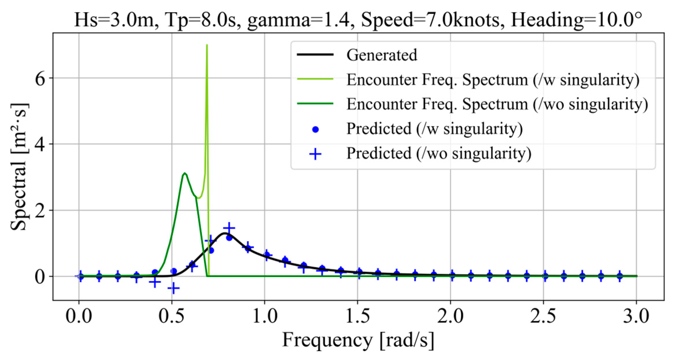
According to Equation (9), the encounter wave spectrum exhibits a singularity when the denominators become zero, leading to an unwanted singularity in the spectrum. This occurs when the frequency approaches ω e = g 4 V c o s β , as indicated by the green line in Figure 3b. However, this singularity may not be captured in the measured spectrum, due to processing steps such as smoothing or insufficient resolution. To represent this case and observe its consequence, we also included the ANN training/validation cases without the sharp peak. It has been observed that a sharp singularity does not significantly affect the performance of the ANN model, as illustrated in Figure 5. This may be due to the fact that the singularity is difficult to detect in the discretized S e ω e . In the ensuing sections, only the results without those singularities are presented.

2.2. Dataset Generation

In the case of a vessel with forward speed, our approach is designed to estimate the wave spectrum from vessel motion sensor signals through the Kalman filter method in the encounter-frequency domain [11,12,15]. In that case, as in the previous section, it was clearly explained that the conversion of the wave spectrum from the encounter-frequency axis to the original-frequency axis may not be unique in the case of following waves and certain vessel speeds. When the spectral conversion from S e ω e to S ω cannot be uniquely determined, we can utilize the present ANN-based ML method, which is demonstrated in the following sections. In that regard, a pair of wave spectra for the original and encounter frequencies are generated using Equations (4), (9), and (10) for various wave parameters and vessel speeds. To demonstrate the workability of the proposed method, the JONSWAP wave parameters and vessel speeds used for the dataset are presented in Table 1. The original and encounter wave spectra are generated with 300 discretized frequency components (Δω = 0.01 rad/s) in the range of angular frequencies of 0 to 3 rad/s. The combination of the wave parameters and vessel speeds generated a total of 231,660 data points.
Figure 6 shows the resulting encounter-frequency spectra generated from the original wave-amplitude spectrum. Various forward speeds and wave headings are considered to provide a comprehensive illustration of the encounter wave characteristics. The various S e ω e values correspond to the same original wave spectrum, which demonstrates why there exists no unique solution in the inverse problem.

2.3. Artificial Neural Network (ANN)

When solving the inverse problem, converting S e ω e to S ω , the problem cannot be solved directly under certain conditions, as explained above, which is the reason we employed the ML approach. Since the relationship between the original and encounter frequency is clearly defined mathematically by the variables of wave heading and forward speed, the neural network model could capture the correlation between S ω and S e ω e with the given wave headings and speeds, enabling the ANN model to potentially recover the original wave spectrum through extensive training for the given instantaneous encounter-frequency spectrum. Figure 7 illustrates a proposed ANN model with its input layer comprising the vessel speed V, angle between the vessel and wave β, and spectral density S e ω e . The output layer includes the discretized original wave spectrum S ω for the original frequency.
Three different models are considered in this paper depending on the selection of the wave parameter and the input variables, as shown in Table 2. Model 1 is an initial model where the peak enhancement factor γ is fixed at 2 for initial testing. For Models 2 and 3, various γ values were considered, increasing the total number of training data points to achieve sufficient model accuracy. Model 2 uses the significant wave height Hs as an additional input variable, assuming that it is obtained from the encounter wave spectrum measured. Meanwhile, Model 3 does not include Hs as the input variable in training the ANN model. A total of 231,660 data points for the respective spectral relations (300 equally spaced points in the range of 0–3 rad/s) between S ω and S e ω e are generated for the ANN scheme of Models 2 and 3. The models are trained using 80% of the total dataset and validated with the remaining 20% of the dataset. During the process, model optimization was performed to adjust the number of layers and nodes, optimizers, and loss functions. The configuration was selected based on preliminary testing, aiming to balance performance and model simplicity. ReLU activation was chosen due to its common effectiveness in regression tasks. The Adam optimizer was selected for its adaptive learning rate, which is generally effective for training nonlinear models such as ANNs. The MSE loss function was used as it is a standard choice for regression tasks and helps penalize larger prediction errors.
An example of hyperparameter optimization, performed using Model 2 with a smaller dataset (totaling 105,300 samples), is presented in Table 3. The R2 score, computed using a 20% validation set, indicated that variations in the tested parameters had a relatively limited impact on model performance. Based on this analysis, the best-performing parameter set was selected and subsequently applied to all models for consistency.
The model errors for each estimated spectrum S ^ are defined by
M A E S , S ^ = 1 n i = 0 n 1 S i S i ^   ( Mean   Absolute   Error ) ,
M S E S , S ^ = 1 n i = 0 n 1 S i S i ^ 2   ( Mean   Squared   Error ) ,
R M S E = M S E S , S ^   ( Root - Mean - Squared   Error ) ,
where n represents the number of discretization points in the frequency domain.
The NRMSE is normalized with the maximum spectral density of the original wave:
N R M S E = R M S E m a x ( S i )
The R2 score, or coefficient of determination, is a common metric used to evaluate the overall performance of the ML models and is defined as
R 2 = 1 i = 1 m y i y i ^ 2 i = 1 m y i y i ¯ 2 ,
where y i is the actual value, y i ^ is the predicted value, y i ¯ is the mean of actual values, and m is the number of data points.
The v.0.3.1 hyperparameter configuration, consisting of three hidden layers with 200 nodes each, was selected based on its highest R2 score and lowest mean NRMSE among the tested variations, while also offering a relatively simple structure to reduce training time.
Additionally, feature-wise data normalization was applied across all models to improve training stability and enhance predictive performance. Min-max normalization was applied to both input and output features using MinMaxScaler, scaling values to the range [0,1]. This helped improve training stability and ensured consistent feature scaling across all models.

3. Results

3.1. ANN Model Performance

The performance of the trained ANN model was evaluated using the R2 score and model errors. Table 4 presents the results of the performance evaluation based on all validation cases, which were drawn from 20% of the dataset and were not included in the 80% used for training. The trained ANN models exhibited sufficient overall accuracy. It is noteworthy that Model 1 achieved high accuracy despite using only 1/10 of the dataset size of Models 2 and 3, due to the fixed peak enhancement factor. The performance of Model 2 was slightly improved when the additional input Hs was employed. However, the performance of Model 3 was as good as that of Model 2, as demonstrated in Figure 8. In the case of S e ω e obtained through motion sensors, the estimation of Hs may be less robust compared to the present numerically evaluated Hs from the theoretically generated S e ω e . Model 3 is more practical and reliable compared to Model 2, as it does not require the real-time estimation of Hs as an additional input. Therefore, from a practical perspective, Model 3 is more suitable, and its accuracy remains sufficiently high. For this reason, we have selected Model 3 for the subsequent discussions.
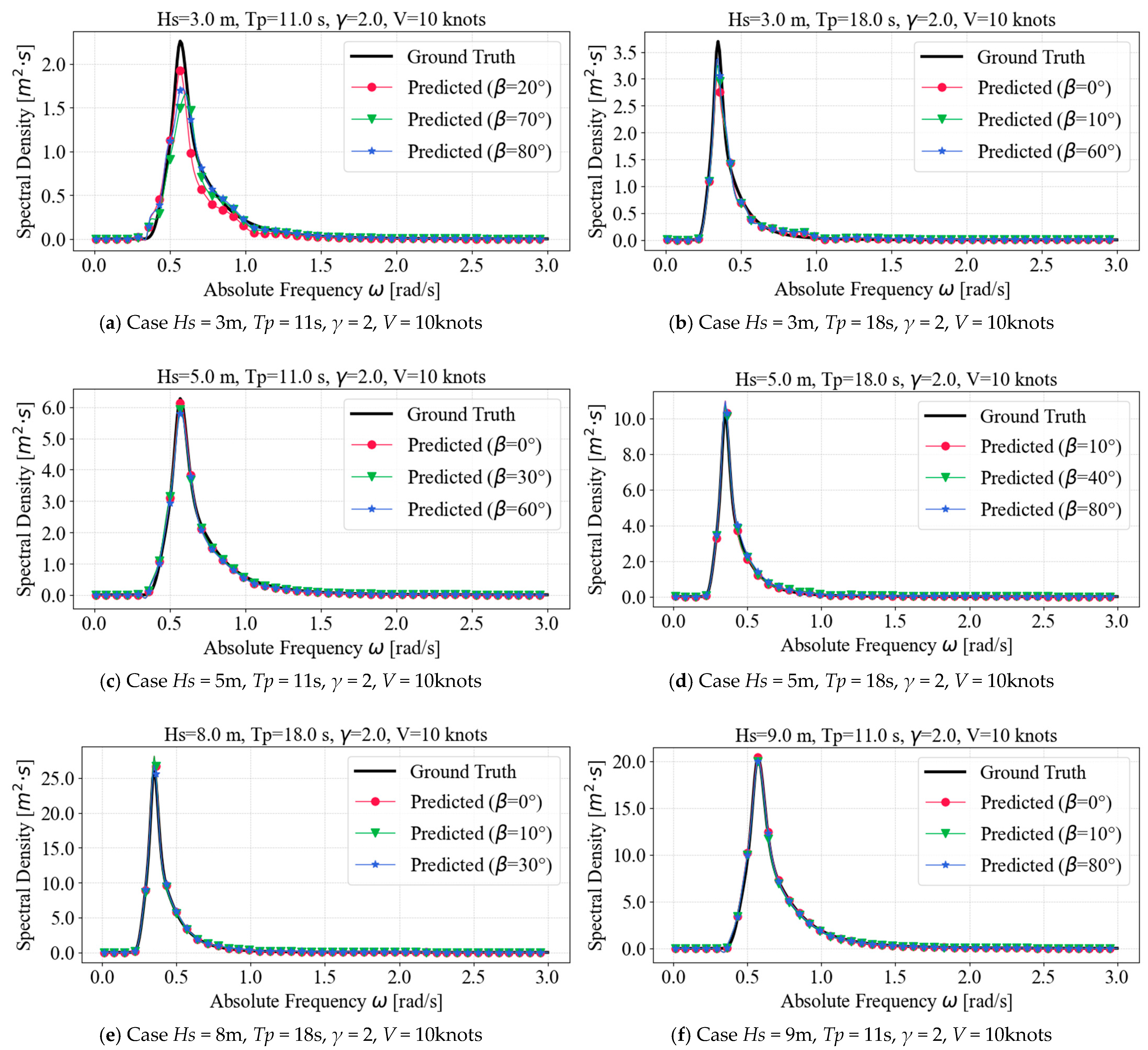
Figure 9 illustrates the estimated wave spectrum using Model 3 for several environmental conditions. The selected validation cases for various Hs, Tp, γ, β, and V values show that the inversely predicted wave spectrum agrees very well with the original wave spectrum. In most conditions, the results demonstrate successful recovery of the original wave spectrum regardless of wave directions and vessel speeds. The wave heading is 40 degrees for this figure. Especially, the peak period is estimated very accurately. Figure 10 also shows the results of Model 3 where the wave heading is changing while V is fixed at 10 knots. This case shows even better performance compared to Figure 9. The small differences in wave spectrum (wave amplitude squared) become even smaller when the corresponding wave elevations are compared.
Figure 11 presents the inversely estimated spectra for different γ values. The recovery of S ω from S e ω e demonstrates strong robustness across various γ values, although slight errors are observed at lower γ values. We also checked many other cases while varying other wave parameters and the results are all similarly good, as presented in Figure 9, Figure 10 and Figure 11.

3.2. Model Error Distribution

The Root-Mean-Squared Error (RMSE) and Normalized RMSE (NRMSE) are employed as evaluation metrics to assess the performance of the trained ANN model. These metrics provide valuable insights into the accuracy of the model predictions across various wave parameters and vessel forward speeds. The RMSE and NRMSE are calculated for the discrete spectral density for each case using Equations (14) and (15), respectively. Figure 12 presents the error distributions observed along the wave parameters and vessel forward speeds. The error distributions are visualized using box plots, which depict the quartiles of the dataset. The whiskers of the box plots (1.5 × IQR) extend to show the rest of the distribution, excluding points identified as outliers. Outliers are identified using a method based on the inter-quartile range (IQR), ensuring robustness in the analysis of the error distributions.
The ANN model demonstrates an RMSE accuracy of less than 0.4, indicating low overall error rates. However, the NRMSE values indicate higher errors with low significant wave heights (Hs) since the magnitude of the spectral density is small in this condition. Notably, for significant wave heights (Hs) greater than or equal to 3 m, the model accuracy is less than 7% in terms of NRMSE. Conversely, for Hs values less than 3 m, the NRMSE values tend to be higher. Other parameters do not show significant variability in the RMSE and NRMSE distribution, but it could be seen that the errors slightly increase at low peak periods (Tp), low peak enhancement factors (γ), high forward speeds (V), and low wave headings (β).
Figure 13 presents a test case that utilizes the estimated encounter wave spectrum obtained via the Kalman filter (KF) algorithm, using real-time motion sensor signals as illustrated in Figure 1. This example demonstrates a more realistic application of ML Model 3, which converts encounter wave spectra experienced by vessels into original wave spectra. The onboard KF-estimated encounter wave spectrum fluctuates and contains some error, as shown in Figure 13a, and therefore requires conversion to the original wave spectrum using the ANN. As a result, the overall accuracy of the reproduced original wave spectrum is slightly reduced compared to the theoretical curves, as shown in Figure 13b. Nevertheless, the overall spectral shape is reconstructed with reasonable accuracy. This result highlights the model’s potential for practical use in real-time onboard applications, even though the initial training was conducted using various theoretical spectra.

3.3. Bimodal Sea State

In cases where the sea state is bimodal (two peaks), comprising both wind sea and swell, the wave spectrum becomes a combination of these two individual sea spectra. It is of interest whether the present ML method can also be applied to this kind of bimodal wave spectra. In this regard, we evaluated the performance of our artificial neural network (ANN) model in predicting the bimodal spectrum with respect to the original-frequency basis using a dataset of both unimodal and bimodal sea conditions. For this model, we generated the dataset comprising 192 unimodal cases and 192 bimodal cases, as outlined in Table 5, which details the wind–sea and swell components. Table 6 provides the parameters used to train the ANN model, which were optimized formerly.
Figure 14 illustrates the results of Model 4 in predicting the absolute frequency spectrum from the encounter spectrum for both unimodal and bimodal sea states. The results show that the applied ML method can predict the bimodal spectrum equally as well as the unimodal spectrum in the original-frequency domain. This example indicates that the present ANN model is robust and versatile even in the case of complex, multi-modal wave conditions.

3.4. Additional Remarks

If only Hs is to be exchanged among ships and marine facilities, the inverse spectral conversion may be unnecessary since Hs can also be obtained from 4 m 0 , where m 0 is the area of S e ω e . However, there may be uncertainty in determining the Tp of S ω inverted from the Tp of S e ω e when ω e < g 4 V c o s β since it can be mapped into three different original wave frequencies. This problem can be resolved by applying the proposed ML-based method. When original wave spectra need to be informed and exchanged among surrounding vessels and facilities, the present method can also be applied, as was demonstrated in the above. In this study, the incident unidirectional random wave spectrum was defined by a typical narrow-banded wave spectrum like the JONSWAP spectrum. However, more diverse patterns of incident wave spectra can be inputted and used for training the ANN algorithm to expand the overall prediction capability. The wave direction can be estimated in real-time by using the KF method and ML method with motion-sensor signals, as detailed in authors’ previous papers [11,12,14,15]. In the case of multi-directional random waves, an additional directional spreading parameter can be employed with increased cases and datasets and the same ML processes can straightforwardly be applied.

4. Summary and Conclusions

In this study, we investigated a data- and ML-based approach for the spectral conversion from the encounter wave frequency spectrum S e ω e to the original-frequency wave spectrum S ω . This conversion is essential when waves and motions are measured from vessel-mounted sensors during navigation with forward speed. The spectral conversion can straightforwardly be performed by an equation in head-wise wave directions, but challenges arise in following-wise wave directions for certain vessel speeds due to the non-unique nature of the inverse problem. To resolve the problem under that condition, we employed an artificial neural network (ANN) model to estimate S ω from S e ω e in a much more robust manner. Vessel speed (V), wave direction (β), and S e ω e values were used as inputs and S ω values were obtained as outputs through the optimization of the ANN frame and hyperparameters. The model was trained using the synthesized data representing a pair of original and encounter wave frequency spectra for various wave parameters, vessel speeds, and wave headings. Our results demonstrated the effectiveness of the ANN model in accurately predicting the original wave spectrum from the encounter wave spectrum when that kind of spectral conversion is not possible. Regardless of various wave conditions and vessel speeds, it was shown that the ANN model robustly predicted the original wave spectrum with sufficient accuracy (R2 value of 0.987). The corresponding error distribution analysis provides valuable insights into the performance of the model across different wave parameters and vessel forward speeds. The applied ML method can also predict the bimodal (two-peaked) spectrum equally as well as the unimodal spectrum in the original-frequency domain. In the present paper, the incident random wave was assumed to be unidirectional. When a multi-directional random wave is considered, we can apply the same method while more wave parameters like directional spreading need to be employed. The proposed spectral transformation method from the encounter to original wave spectra is designed to be general and independent of specific ship types. However, the Kalman filter (KF) method introduced earlier in the manuscript does rely on ship-specific motion characteristics, as it uses the vessel’s response amplitude operator (RAO) to reconstruct the wave spectrum in a vessel-specific manner.

Author Contributions

Conceptualization, J.P. and M.K.; methodology, J.P. and M.K.; software, J.P.; validation, J.P.; formal analysis, J.P. and M.K.; investigation, J.P. and M.K.; data curation, J.P.; writing—original draft preparation, J.P.; writing—review and editing, M.K.; visualization, J.P.; supervision, M.K. All authors have read and agreed to the published version of the manuscript.

Funding

This research received no external funding.

Institutional Review Board Statement

Not applicable.

Informed Consent Statement

Not applicable.

Data Availability Statement

The raw data supporting the conclusions of this article will be made available by the authors on request.

Conflicts of Interest

The authors declare no conflicts of interest.

Abbreviations

The following abbreviations are used in this manuscript:
MLMachine Learning
ANNArtificial Neural Network
JONSWAPJoint North Sea Wave Project
ECMWFEuropean Centre for Medium-Range Weather Forecasts
NCEPNational Centers for Environmental Prediction
KFKalman Filter
RAOResponse Amplitude Operator
MAEMean Absolute Error
MSEMean Squared Error
RMSERoot-Mean-Squared Error
NRMSENormalized Root-Mean-Squared Error
IQRInter-Quartile Range

References

  1. Kim, S. The development of route decision-making method based on tailor-made forecast 2d wave spectra due to the operation profile of the vessel. Ocean Eng. 2020, 197, 106907. [Google Scholar]
  2. Vettor, R.; Soares, C.G. Development of a ship weather routing system. Ocean Eng. 2016, 123, 1–14. [Google Scholar]
  3. Caamaño, L.S.; González, M.M.; Casás, V.D. Improving the performance of a stability monitoring system by adding wave encounter frequency estimation. IFAC-PapersOnLine 2022, 55, 320–326. [Google Scholar] [CrossRef]
  4. Han, X.; Leira, B.J.; Sævik, S.; Ren, Z. Onboard tuning of vessel seakeeping model parameters and sea state characteristics. Mar. Struct. 2021, 78, 102998. [Google Scholar] [CrossRef]
  5. Natskår, A.; Moan, T.; Alvær, P.Ø. Uncertainty in forecasted environmental conditions for reliability analyses of marine operations. Ocean Eng. 2015, 108, 636–647. [Google Scholar]
  6. Stredulinsky, D.C.; Thornhill, E.M. Ship motion and wave radar data fusion for shipboard wave measurement. J. Ship Res. 2011, 55, 73–85. [Google Scholar] [CrossRef]
  7. Felski, A.; Zwolak, K. The ocean-going autonomous ship—Challenges and threats. J. Mar. Sci. Eng. 2020, 8, 41. [Google Scholar] [CrossRef]
  8. Thombre, S.; Zhao, Z.; Ramm-Schmidt, H.; García, J.M.V.; Malkamäki, T.; Nikolskiy, S.; Hammarberg, T.; Nuortie, H.; Bhuiyan, M.Z.H.; Särkkä, S. Sensors and AI techniques for situational awareness in autonomous ships: A review. IEEE Trans. Intell. Transp. Syst. 2020, 23, 64–83. [Google Scholar] [CrossRef]
  9. Iseki, T.; Ohtsu, K. Bayesian estimation of directional wave spectra based on ship motions. Control Eng. Pract. 2000, 8, 215–219. [Google Scholar]
  10. Nielsen, U.D. Estimations of on-site directional wave spectra from measured ship responses. Mar. Struct. 2006, 19, 33–69. [Google Scholar] [CrossRef]
  11. Kim, H.; Kang, H.; Kim, M.-H. Real-time inverse estimation of ocean wave spectra from vessel-motion sensors using adaptive kalman filter. Appl. Sci. 2019, 9, 2797. [Google Scholar] [CrossRef]
  12. Kim, H.; Park, J.; Jin, C.; Kim, M.; Lee, D. Real-time inverse estimation of multi-directional random waves from vessel-motion sensors using Kalman filter. Ocean Eng. 2023, 280, 114501. [Google Scholar]
  13. Pascoal, R.; Perera, L.P.; Soares, C.G. Estimation of directional sea spectra from ship motions in sea trials. Ocean Eng. 2017, 132, 126–137. [Google Scholar] [CrossRef]
  14. Kwon, D.-S.; Jin, C.; Kim, M.; Guha, A.; Esenkov, O.E.; Ryu, S. Inverse wave estimation from measured FPSO motions through artificial neural networks. In Proceedings of the SNAME Offshore Symposium, Houston, Texas, USA, 20 February 2024; p. D011S004R003. [Google Scholar]
  15. Kwon, D.-S.; Jin, C.; Kim, S.-J.; Kim, M.; Guha, A.; Gosain, G.; Ryu, S.; Ferreira, M.D.; Auburtin, E.; Minnebo, J. Inverse Ocean Wave Estimation from FPSO Motions by Artificial Neural Network. In Proceedings of the ISOPE International Ocean and Polar Engineering Conference, Ottawa, Canada, 19–23 June 2023; p. ISOPE-I-23-146. [Google Scholar]
  16. Nielsen, U.D.; Mittendorf, M.; Shao, Y.; Storhaug, G. Wave spectrum estimation conditioned on machine learning-based output using the wave buoy analogy. Mar. Struct. 2023, 91, 103470. [Google Scholar] [CrossRef]
  17. Iseki, T. Extended Bayesian estimation of directional wave spectra. In Proceedings of the International Conference on Offshore Mechanics and Arctic Engineering, Vancouver, BC, Canada, 20–25 June 2004; pp. 611–616. [Google Scholar]
  18. Brodtkorb, A.H.; Nielsen, U.D. Automatic sea state estimation with online trust measure based on ship response measurements. Control Eng. Pract. 2023, 130, 105375. [Google Scholar] [CrossRef]
  19. Iseki, T. Real-time estimation of directional wave spectra using non-stationary ship motion data. In Proceedings of the International Conference on Offshore Mechanics and Arctic Engineering, Honolulu, HI, USA, 31 May–5 June 2009; pp. 673–678. [Google Scholar]
  20. Nielsen, U.D.; Iseki, T. Estimation of Sea State Parameters From Measured Ship Responses: The Bayesian Approach With Fixed Hyperparameters. In Proceedings of the International Conference on Offshore Mechanics and Arctic Engineering, Shanghai, China, 6–11 June 2010; pp. 23–32. [Google Scholar]
  21. Faltinsen, O. Sea Loads on Ships and Offshore Structures; Cambridge University Press: Cambridge, UK, 1993; Volume 1. [Google Scholar]
  22. Nielsen, U.D. Transformation of a wave energy spectrum from encounter to absolute domain when observing from an advancing ship. Appl. Ocean Res. 2017, 69, 160–172. [Google Scholar] [CrossRef]
  23. Nielsen, U.D. Deriving the absolute wave spectrum from an encountered distribution of wave energy spectral densities. Ocean Eng. 2018, 165, 194–208. [Google Scholar] [CrossRef]
  24. Hasselmann, K.; Barnett, T.P.; Bouws, E.; Carlson, H.; Cartwright, D.E.; Enke, K.; Ewing, J.; Gienapp, A.; Hasselmann, D.; Kruseman, P. Measurements of Wind-Wave Growth and Swell Decay During the Joint North Sea Wave Project (JONSWAP). “Ergänzungsheft zur Deutschen Hydrographischen Zeitschrift, Reihe A, Nr. 12.”. 1973. Available online: https://hdl.handle.net/21.11116/0000-0007-DD3C-E (accessed on 27 January 2025).
  25. DNV. Recommended Practice DNV-RP-C205: Environmental Conditions and Environmental Loads; DNV: Høvik, Norway, 2010. [Google Scholar]
Figure 1. Estimated unidirectional wave spectrum using Kalman filter with simulated motion time series with and without forward speed (significant wave height Hs = 5 m, peak periods Tp = 9 s, peak enhancement factor γ = 2, and wave heading β = 0°): (a) no forward speed; (b) forward speed V = 5 knots.
Applsci 15 03987 g001
Figure 2. Relationship between original and encounter frequencies for following/quartering sea.
Applsci 15 03987 g002
Figure 3. Encounter wave frequency conversion (Hs = 5 m, Tp = 9 s, β = 30°, and V = 7 knots): (a) original vs. encounter frequency; (b) recovered spectrum.
Applsci 15 03987 g003
Figure 4. Encounter wave frequency conversion (Hs = 5 m, Tp = 9 s, β = 30°, and V = 15 knots): (a) original vs. encounter frequency; (b) recovered spectrum.
Applsci 15 03987 g004
Figure 5. Estimated original wave spectrum from encounter wave spectrum with and without singularity.
Applsci 15 03987 g005
Figure 6. Encountered wave spectra (Hs = 3 m, Tp = 7 s, γ = 2) with corresponding (a) forward speeds (β = 40 deg) and (b) wave headings (V = 16 knots).
Applsci 15 03987 g006
Figure 7. Artificial neural network (ANN) model for wave encounter-frequency conversion.
Applsci 15 03987 g007
Figure 8. Comparison of estimated original wave spectra through Model 2 and Model 3.
Applsci 15 03987 g008
Figure 9. Estimated original wave spectra at different forward speeds V (Model 3, heading β = 40 deg, and peak enhancement factor γ = 2).
Applsci 15 03987 g009
Figure 10. Estimated original wave spectra at different wave headings β (Model 3, forward speed V = 10 knots, and peak enhancement factor γ = 2).
Applsci 15 03987 g010
Figure 11. Estimated original wave spectra at different peak enhancement factors γ (Model 3, Hs = 3 m, Tp = 15 m, wave headings β = 30 deg, and forward speed V = 10 knots).
Applsci 15 03987 g011
Figure 12. Error distribution of Model 3 for wave parameters.
Applsci 15 03987 g012
Figure 13. Encounter wave frequency spectrum (theoretical vs. estimated) and ANN-predicted original wave spectrum (Hs = 5 m, Tp = 9 m, peak enhancement factor γ = 2, wave headings β = 0 deg, and forward speed V = 7 knots).
Applsci 15 03987 g013
Figure 14. Estimated original wave spectra of bimodal sea (Model 4).
Applsci 15 03987 g014
Table 1. Wave parameters and vessel forward speeds for dataset.
JONSWAP Wave ParameterRange of ValuesInterval
Hs, significant wave height (m)[1, 2, …, 9]1 m
Tp, peak period (s)[6, 7, …, 18]1 s
γ, peak enhancement factor *[1, 1.2, …, 3]0.2
β, wave heading (deg) **[0, 10, …, 80]10°
V, forward speed (knots)[1, 2, …, 20]1 m/s
* For ML Model 1, the peak enhancement factor γ is fixed to 2. ** A wave heading of 0 degrees represents the following sea, while a heading of 90 degrees means the beam sea.
Table 2. Artificial neural network (ANN) model parameters.
ANN Model ParameterModel 1Model 2Model 3
Number of layers333
Number of neurons (per layer)200200200
Activation functionReLUReLUReLU
OptimizerAdam *Adam Adam
Loss functionMSE **MSEMSE
Input variables V ,   β ,   S e ω e Hs * * * ,   V ,   β ,   S e ω e V ,   β ,   S e ω e
Output variables S ( ω ) S ( ω ) S ( ω )
Total dataset21,060 ****231,660231,660
Remarkγ = 2 (fixed)γ = range of 1–3γ = range of 1–3
* Learning rate: 0.001. ** Mean Squared Error. *** It is assumed that Hs is known with Hs =   4 m 0 , where m 0 is the zeroth moment of the encounter-frequency spectrum. **** The amount of data for training is less than those of Models 2 and 3 as the peak enhancement factor is fixed for initial testing.
Table 3. Hyperparameter optimization for ML Model 2.
Model
Optimization
R2 ScoreNRMSE Mean *LayerNodesOptimizerLoss FunctionEpochs
v.00.9840.71%350adamMSE25
v.0.10.9850.70%3100adamMSE25
v.0.1.10.9890.54%3100adamMSE50
v.0.20.9890.52%3150adamMSE25
v.0.2.10.9870.64%3150adamMSE50
v.0.2.20.9880.54%3150adamMSE100
v.0.30.9870.60%3200adamMSE25
v.0.3.10.9910.47%3200adamMSE50
v.0.3.20.9880.64%3200adamMSE100
v.0.3.2.10.9870.56%2200adamMSE100
v.0.3.2.20.9910.47%4200adamMSE100
v.0.3.2.30.9880.56%5200adamMSE100
v.0.3.30.9910.48%3200adamMSE150
v.0.4.20.9890.54%3300adamMSE100
* The mean NRMSE is calculated using the NRMSE values from all validation sets.
Table 4. Artificial neural network (ANN) model metrics.
ANN Model MetricsModel 1Model 2Model 3
MAE (Mean Absolute Error)0.0460.0520.059
MSE (Mean Squared Error)0.0250.0250.045
RMSE (Root-Mean-Squared Error)0.1590.1590.213
R Square (R2)0.9930.9930.987
Table 5. JONSWAP wave parameters for Model 4 dataset.
JONSWAP Wave ParameterValues
Hs, wind sea (m)[2.5, 3.5]
Hs, swell (m)[0 *, 3, 4]
Tp, wind sea (s)[5, 7]
Tp, swell (s)[10, 11]
γ, wind sea[1, 2]
γ, swell[4, 5]
β (deg)[5, 10]
V (knots)[10, 40]
* Hs = 0 for unimodal seas.
Table 6. ANN Model 4 parameters.
ANN Model ParameterModel 4
Number of layers3
Number of neurons (per each layer)200
Activation functionReLu
OptimizerAdam (Learning rate: 0.001)
Loss functionMSE (Mean Squared Error)
Input variables V ,   β ,   S e ω e
Output variables S ( ω )
Total dataset384 (192 unimodal + 192 bimodal seas)
Disclaimer/Publisher’s Note: The statements, opinions and data contained in all publications are solely those of the individual author(s) and contributor(s) and not of MDPI and/or the editor(s). MDPI and/or the editor(s) disclaim responsibility for any injury to people or property resulting from any ideas, methods, instructions or products referred to in the content.