

An Alternative Procedure for the Description of Seismic Intensity Parameter-Based Damage Potential


Abstract
1. Introduction
2. Methods
2.1. Seismic Intensity Measures
2.2. Seismic Acceleration Time Histories

| Intensity Measure | Symbol | Units | Minimum | Maximum | Average | Standard Deviation | References |
|---|---|---|---|---|---|---|---|
| Housner Intensity | SIH | cm | 15.410 | 673.467 | 161.324 | 135.671 | [30] |
| Sa,avg | Sa,avg | g | 0.030 | 1.282 | 0.372 | 0.299 | [31] |
| Specific Energy Density | SED | cm2/s | 11.378 | 68,792.353 | 5602.030 | 10,271.634 | [32] |
| Velocity Spectrum Intensity | SIv | cm | 21.460 | 635.346 | 180.210 | 134.699 | [33] |
| PGV | PGV | cm/s | 5.929 | 222.942 | 49.955 | 39.445 | [3] |
| Sv,T1(5%) | Sv,T1(5%) | cm/s | 9.811 | 364.923 | 84.838 | 73.964 | [3] |
| Sa,T1(5%) | Sa,T1(5%) | g | 0.015 | 1.991 | 0.385 | 0.382 | [3] |
| Sd,T1(5%) | Sd,T1(5%) | cm | 0.565 | 76.975 | 14.855 | 14.775 | [3] |
| Sustained Maximum Velocity | SMV | cm/s | 1.765 | 135.907 | 33.653 | 27.657 | [34] |
| Velocity RMS | vRMS | cm/s | 0.291 | 39.986 | 8.058 | 7.404 | [4] |
| Max Incremental Velocity | MIV | cm/s | 7.478 | 308.843 | 72.813 | 55.261 | [35,36] |
| PGD | PGD | cm | 0.451 | 111.511 | 17.283 | 22.265 | [3] |
| Displacement RMS | dRMS | cm | 0.030 | 28.531 | 4.163 | 5.876 | [4] |
| vmax/amax | vmax/amax | s | 0.017 | 0.436 | 0.093 | 0.069 | [37] |
| Mean Period | Tm | s | 0.102 | 1.479 | 0.498 | 0.288 | [38] |
| Standardized CAV | CAVstd | g∙s | 0.000 | 4.776 | 1.217 | 1.019 | [39] |
| Cumulative Absolute Velocity | CAV | cm | 135.287 | 5062.353 | 1382.785 | 1063.057 | [40] |
| Arias Intensity | IA | m/s | 0.109 | 18.247 | 3.649 | 3.641 | [27] |
| Characteristic Intensity | IC | g1.5∙s0.5 | 0.007 | 0.431 | 0.120 | 0.090 | [3] |
| Predominant Period | Tp | s | 0.060 | 1.120 | 0.330 | 0.235 | [3] |
| Acceleration RMS | aRMS | g | 0.007 | 0.221 | 0.068 | 0.039 | [41] |
| Sustained Maximum Acceleration | SMA | g | 0.042 | 1.190 | 0.370 | 0.202 | [34] |
| Acceleration Spectrum Intensity | SIa | g∙s | 0.078 | 1.183 | 0.436 | 0.212 | [33] |
| Uniform Duration | tuniform | s | 1.340 | 61.975 | 12.551 | 9.899 | [26,42] |
| Bracketed Duration | tbracketed | s | 2.780 | 159.970 | 27.943 | 23.404 | [43] |
| Significant Duration | tsignificant | s | 0.760 | 51.200 | 10.625 | 8.906 | [26] |
| Effective Design Acceleration | EDA | g | 0.120 | 1.644 | 0.548 | 0.240 | [40] |
| PGA | PGA | g | 0.121 | 1.647 | 0.566 | 0.257 | [3] |
| Power 0.90 | P0.90 | m/s2 | 0.013 | 2.199 | 0.404 | 0.412 | [44] |
| Damage Index | D | - | 0.166 | 51.713 | 6.466 | 8.568 | [45,46] |
| A95 parameter | A95 | g | 0.084 | 1.332 | 0.409 | 0.188 | [32] |
| Number of Effective Cycles | Ncy | - | 0.679 | 17.025 | 3.277 | 2.873 | [45,46] |
| Total Duration | ttotal | s | 1.375 | 299.990 | 54.191 | 46.780 | [3] |
| IP Index | IP | - | 7.194 | 265.740 | 33.462 | 26.118 | [47] |
| RSN | Seismic Event | Station | Magnitude | Hypocenter Depth (km) | Epicentral Distance (km) | Vs30 (m/s) | Components |
|---|---|---|---|---|---|---|---|
| 1 | Helena, Montana-01 | Carroll College | 6.00 | 6.00 | 6.31 | 593.35 | 180, 270 |
| 15 | Kern County | Taft Lincoln School | 7.36 | 15.63 | 43.49 | 385.43 | 21, 111 |
| 33 | Parkfield | Temblor pre-1969 | 6.19 | 10.00 | 40.25 | 527.92 | 205, 295 |
| 50 | Lytle Creek | Wrightwood—6074 Park Dr | 5.33 | 8.00 | 13.01 | 486.00 | 115, 205 |
| 57 | San Fernando | Castaic—Old Ridge Route | 6.61 | 13.00 | 25.36 | 450.28 | 21, 291 |
| 125 | Friuli, Italy-01 | Tolmezzo | 6.50 | 5.10 | 20.24 | 505.23 | 0, 270 |
| 134 | Izmir, Turkey | Izmir | 5.30 | 5.00 | 2.29 | 535.24 | L, T |
| 136 | Santa Barbara | Santa Barbara Courthouse | 5.92 | 12.70 | 3.20 | 514.99 | 132, 222 |
| 139 | Tabas, Iran | Dayhook | 7.35 | 5.75 | 20.63 | 471.53 | 190, 280 |
| 143 | Tabas, Iran | Tabas | 7.35 | 5.75 | 55.24 | 766.77 | 74, 344 |
| 150 | Coyote Lake | Gilroy Array #6 | 5.74 | 8.00 | 4.37 | 663.31 | 230, 320 |
| 182 | Imperial Valley-06 | El Centro Array #7 | 6.53 | 9.96 | 27.64 | 210.51 | 140, 230 |
| 214 | Livermore-01 | San Ramon—Eastman Kodak | 5.80 | 12.00 | 17.13 | 377.51 | 180, 270 |
| 222 | Livermore-02 | Livermore—Morgan Terr Park | 5.42 | 14.50 | 10.33 | 550.88 | 265, 355 |
| 225 | Anza (Horse Canyon)-01 | Anza—Pinyon Flat | 5.19 | 13.60 | 12.68 | 724.89 | 45, 135 |
| 230 | Mammoth Lakes-01 | Convict Creek | 6.06 | 9.00 | 1.43 | 382.12 | 90, 180 |
| 233 | Mammoth Lakes-02 | Convict Creek | 5.69 | 14.00 | 8.60 | 382.12 | 90, 180 |
| 244 | Mammoth Lakes-05 | Convict Creek | 5.70 | 4.70 | 9.36 | 382.12 | 90, 180 |
| 246 | Mammoth Lakes-06 | Benton | 5.94 | 14.00 | 46.49 | 370.94 | 0, 270 |
| 256 | Mammoth Lakes-07 | USC McGee Creek Inn | 4.73 | 6.00 | 1.33 | 364.84 | 0, 270 |
| 265 | Victoria, Mexico | Cerro Prieto | 6.33 | 11.00 | 33.73 | 471.53 | 45, 315 |
| 292 | Irpinia, Italy-01 | Sturno (STN) | 6.90 | 9.50 | 30.35 | 382.00 | 0, 270 |
| 313 | Corinth, Greece | Corinth | 6.60 | 7.15 | 19.92 | 361.40 | L, T |
| 359 | Coalinga-01 | Parkfield—Vineyard Cany 1E | 6.36 | 4.60 | 34.35 | 381.27 | 0, 90 |
| 372 | Coalinga-02 | Anticline Ridge Free-Field | 5.09 | 12.00 | 3.38 | 478.63 | 0, 270 |
| 415 | Coalinga-05 | Transmitter Hill | 5.77 | 7.40 | 5.99 | 477.25 | 0, 270 |
| 419 | Coalinga-07 | Sulphur Baths (temp) | 5.21 | 8.40 | 12.02 | 617.43 | 0, 90 |
| 495 | Nahanni, Canada | Site 1 | 6.76 | 8.00 | 6.80 | 605.04 | 10, 280 |
| 534 | N. Palm Springs | San Jacinto—Soboba | 6.06 | 11.00 | 33.53 | 447.22 | 0, 90 |
| 548 | Chalfant Valley-02 | Benton | 6.19 | 10.00 | 31.25 | 370.94 | 0, 270 |
| 550 | Chalfant Valley-02 | Bishop—Paradise Lodge | 6.19 | 10.00 | 15.42 | 585.12 | 70, 160 |
| 564 | Kalamata, Greece-01 | Kalamata (bsmt) | 6.20 | 5.00 | 9.97 | 382.21 | 0, 270 |
| 568 | San Salvador | Geotech Investig Center | 5.80 | 10.90 | 7.93 | 489.34 | 90, 180 |
| 572 | Taiwan SMART1(45) | SMART1 E02 | 7.30 | 15.00 | 71.35 | 671.52 | 0, 90 |
| 585 | Baja California | Cerro Prieto | 5.50 | 6.00 | 3.69 | 471.53 | 161, 251 |
| 619 | Whittier Narrows-01 | Garvey Res.—Control Bldg | 5.99 | 14.60 | 2.86 | 468.18 | 60, 330 |
| 708 | Whittier Narrows-02 | Altadena—Eaton Canyon | 5.27 | 13.30 | 13.04 | 375.16 | 0, 90 |
| 727 | Superstition Hills-02 | Superstition Mtn Camera | 6.54 | 9.00 | 7.50 | 362.38 | 45, 135 |
| 779 | Loma Prieta | LGPC | 6.93 | 17.48 | 18.46 | 594.83 | 0, 90 |
| 802 | Loma Prieta | Saratoga—Aloha Ave | 6.93 | 17.48 | 27.23 | 380.89 | 0, 90 |
| 818 | Georgia, USSR | Iri | 6.20 | 6.00 | 40.23 | 437.72 | X, Y |
| 821 | Erzican, Turkey | Erzincan | 6.69 | 9.00 | 8.97 | 352.05 | 0, 90 |
| 825 | Cape Mendocino | Cape Mendocino | 7.01 | 9.50 | 10.36 | 567.78 | 0, 90 |
| 830 | Cape Mendocino | Shelter Cove Airport | 7.01 | 9.50 | 36.28 | 518.98 | 0, 90 |
| 864 | Landers | Joshua Tree | 7.28 | 7.00 | 13.67 | 379.32 | 0, 90 |
| 881 | Landers | Morongo Valley Fire Station | 7.28 | 7.00 | 21.34 | 396.41 | 45, 135 |
| 901 | Big Bear-01 | Big Bear Lake—Civic Center | 6.46 | 13.00 | 10.15 | 430.36 | 0, 270 |
| 963 | Northridge-01 | Castaic—Old Ridge Route | 6.69 | 17.50 | 40.68 | 450.28 | 0, 90 |
| 982 | Northridge-01 | Jensen Filter Plant Administrative Building | 6.69 | 17.50 | 12.97 | 373.07 | 22, 292 |
| 1111 | Kobe, Japan | Nishi-Akashi | 6.90 | 17.90 | 8.70 | 609.00 | 0, 90 |
| 1114 | Kobe, Japan | Port Island (0 m) | 6.90 | 17.90 | 19.25 | 198.00 | 0, 90 |
| 1231 | Chi-Chi, Taiwan | CHY080 | 7.62 | 8.00 | 31.65 | 496.21 | 0, 90 |
| 1504 | Chi-Chi, Taiwan | TCU067 | 7.62 | 8.00 | 28.70 | 433.63 | 0, 90 |
| 1618 | Duzce, Turkey | Lamont 531 | 7.14 | 14.00 | 27.74 | 638.39 | 0, 90 |
| 1623 | Stone Canyon | Melendy Ranch | 4.81 | 8.00 | 10.19 | 425.11 | 61, 331 |
| 1632 | Upland | Rancho Cucamonga—Law and Justice Center FF, Foothill and Haven | 5.63 | 4.49 | 12.19 | 390.18 | 0, 90 |
| 1633 | Manjil, Iran | Abbar | 7.37 | 16.00 | 40.43 | 723.95 | L, T |
| 1676 | Northridge-04 | Castaic—Old Ridge Route | 5.93 | 9.83 | 26.95 | 450.28 | 0, 90 |
| 1734 | Northridge-06 | Sun Valley—Sunland | 5.28 | 13.09 | 10.04 | 393.67 | 230, 320 |
| 1787 | Hector Mine | Hector | 7.13 | 14.80 | 26.53 | 726.00 | 0, 90 |
| 1948 | Anza-02 | La Quinta—Bermudas and Durango | 4.92 | 15.20 | 26.88 | 360.32 | 0, 90 |
| 2383 | Chi-Chi, Taiwan-02 | TCU067 | 5.90 | 8.00 | 33.94 | 433.63 | 0, 90 |
| 2495 | Chi-Chi, Taiwan-03 | CHY080 | 6.20 | 7.80 | 29.48 | 496.21 | 0, 90 |
| 3217 | Chi-Chi, Taiwan-05 | TCU129 | 6.20 | 10.00 | 40.98 | 511.18 | 0, 90 |
| 3507 | Chi-Chi, Taiwan-06 | TCU129 | 6.30 | 16.00 | 33.15 | 511.18 | 0, 90 |
| 3689 | Whittier Narrows-02 | Big Tujunga, Angeles Nat F | 5.27 | 13.30 | 27.52 | 550.11 | 262, 352 |
| 3733 | Whittier Narrows-02 | Pasadena—Old House Rd | 5.27 | 13.30 | 12.25 | 397.27 | 0, 90 |
| 3748 | Cape Mendocino | Ferndale Fire Station | 7.01 | 9.50 | 27.85 | 387.95 | 0, 270 |
| 3764 | Northridge-02 | LA—UCLA Grounds | 6.05 | 6.00 | 23.53 | 398.42 | 0, 90 |
| 3779 | Northridge-06 | Glendale—Las Palmas | 5.28 | 13.09 | 22.72 | 371.07 | 177, 267 |
| 3845 | Chi-Chi (aftershock 2), Taiwan | CHY006 | 6.20 | 7.80 | 39.60 | 438.19 | 0, 270 |
| 3865 | Chi-Chi (aftershock 5), Taiwan | CHY006 | 6.30 | 16.00 | 56.64 | 438.19 | 0, 270 |
| 4031 | San Simeon, CA | Templeton—1-story Hospital | 6.5 | 8.50 | 36.63 | 410.66 | 0, 90 |
| 4040 | Bam, Iran | Bam | 6.6 | 6.00 | 12.59 | 487.40 | 8, 278 |
| 4097 | Parkfield-02, CA | Slack Canyon | 6.00 | 8.10 | 31.53 | 648.09 | 0, 90 |
| 4114 | Parkfield-02, CA | Parkfield—Fault Zone 11 | 6.00 | 8.10 | 9.28 | 541.73 | 0, 90 |
| 4284 | Basso Tirreno, Italy | Naso | 6 | 15.00 | 18.04 | 620.56 | 0, 90 |
| 4456 | Montenegro, Yugo. | Petrovac—Hotel Olivia | 7.10 | 7.00 | 28.30 | 543.26 | 0, 90 |
| 4861 | Chuetsu-oki | Nakanoshima Nagaoka | 6.80 | 9.00 | 23.28 | 319.00 | 0, 90 |
| 5663 | Iwate | MYG004 | 6.90 | 6.50 | 35.40 | 479.37 | 0, 90 |
| 5819 | Iwate | Ichinoseki Maikawa | 6.90 | 6.50 | 30.72 | 640.14 | 0, 90 |
| 5823 | El Mayor-Cucapah | Chihuahua | 7.20 | 5.45 | 20.63 | 242.05 | 0, 90 |
| 6059 | Big Bear-01 | Morongo Valley Fire Station | 6.46 | 13.00 | 29.33 | 396.41 | 45, 135 |
| 6952 | Darfield, New Zealand | Papanui High School | 7.00 | 10.90 | 46.94 | 263.20 | 123, 213 |
| 8157 | Christchurch, New Zealand | Heathcote Valley Primary School | 6.2 | 6.00 | 1.11 | 422.00 | 116, 206 |
| 8169 | San Juan Bautista | San Andreas Geophysical Obs., Hollister, CA, USA | 5.17 | 9.13 | 1.79 | 643.80 | 0, 90 |
| 9071 | 14151344 | Pinon Flats Observatory, CA, USA | 5.20 | 15.48 | 13.47 | 763.00 | 0, 90 |
| 11133 | 21530368 | Sonoma Mountain | 4.50 | 6.99 | 2.19 | 664.57 | 0, 90 |
| 12261 | 40199209 | Oakland—Hwys 13 and 24 | 4.20 | 4.13 | 6.02 | 511.12 | 0, 90 |
| 20125 | 40204628 | Coe Ranch | 5.45 | 7.49 | 21.25 | 400.00 | 0, 90 |
2.3. Damage Indices
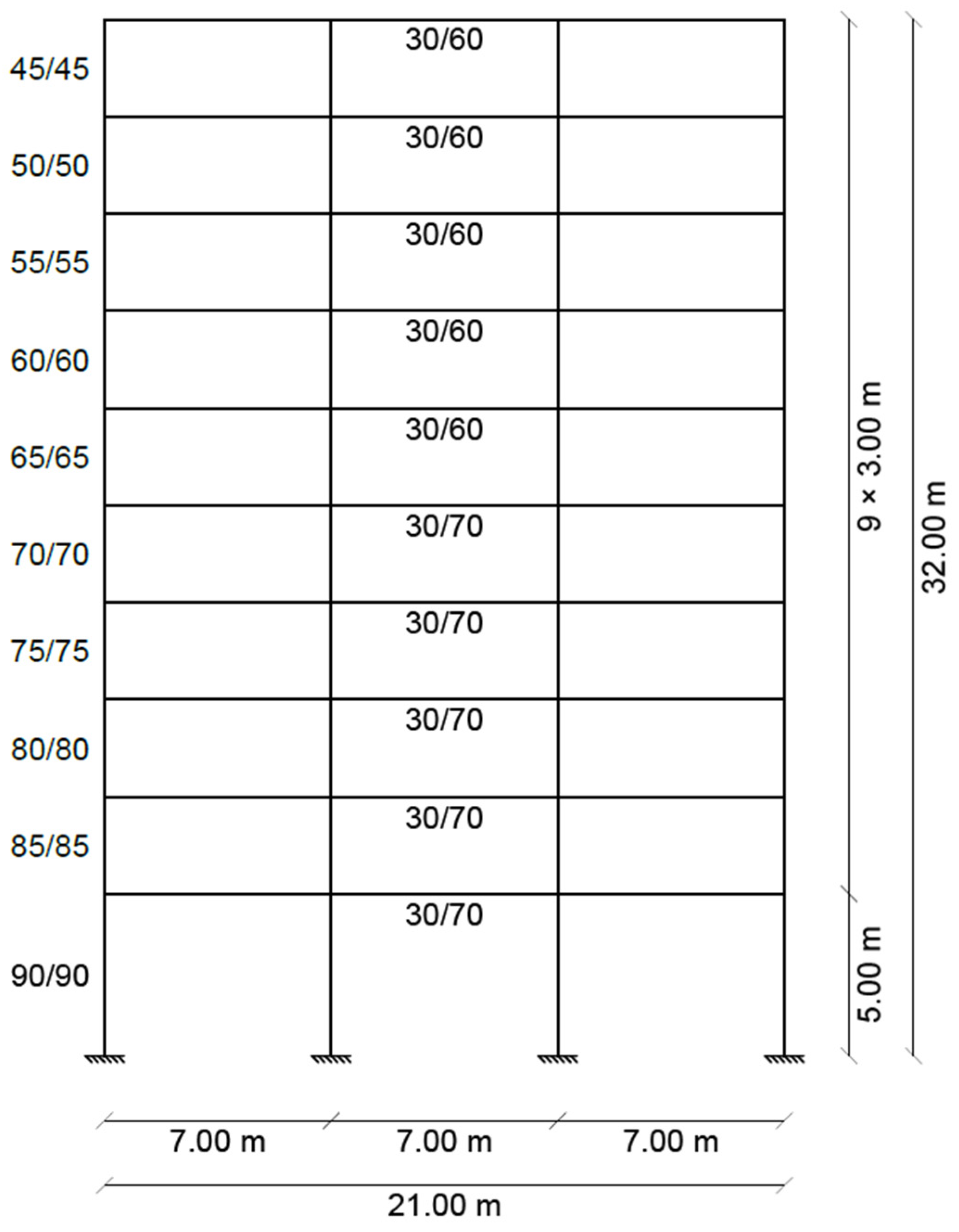
2.4. Numerical Modelling and Investigation on a Reinforced Concrete Frame Structure
2.5. Multiple Regression Analysis
3. Results and Discussion
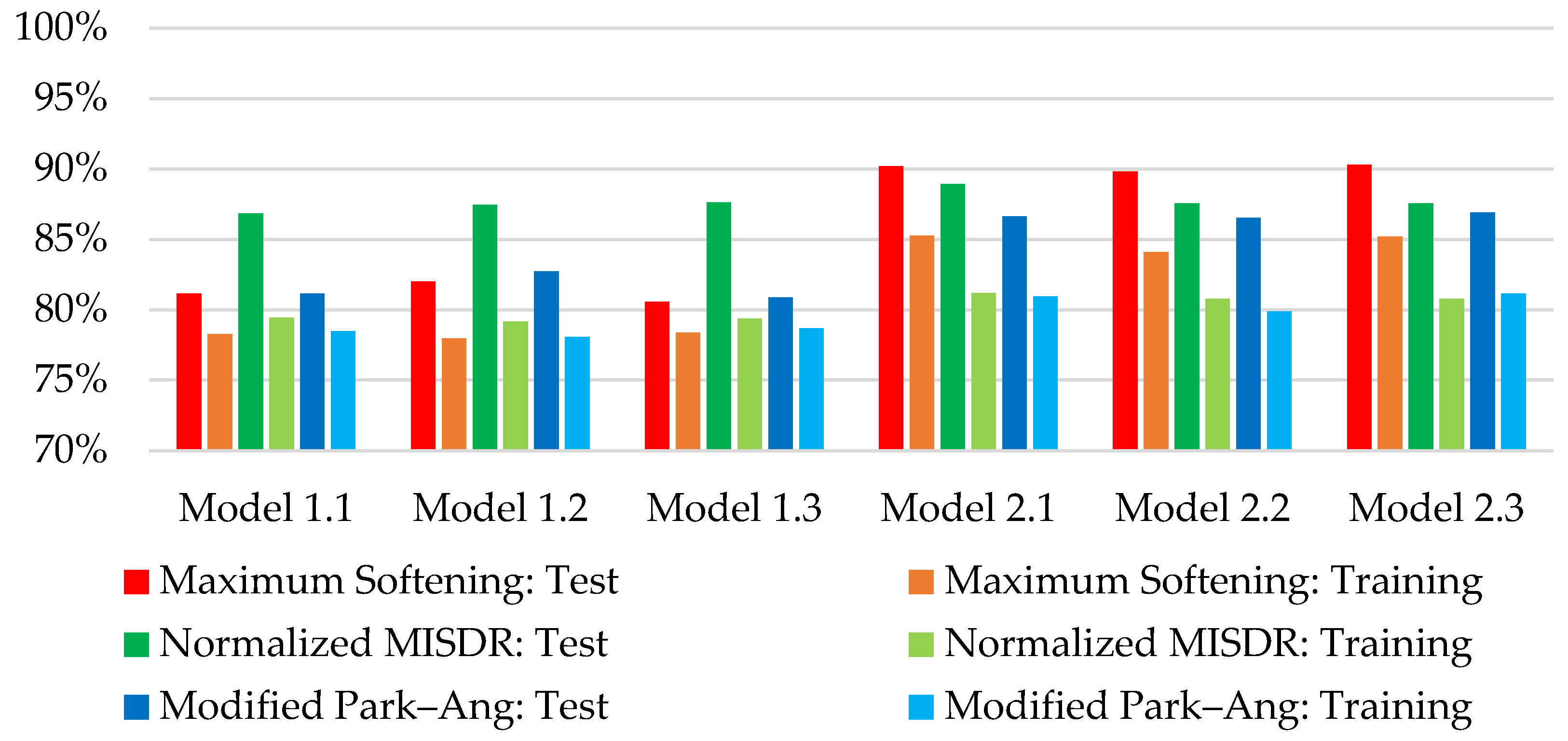
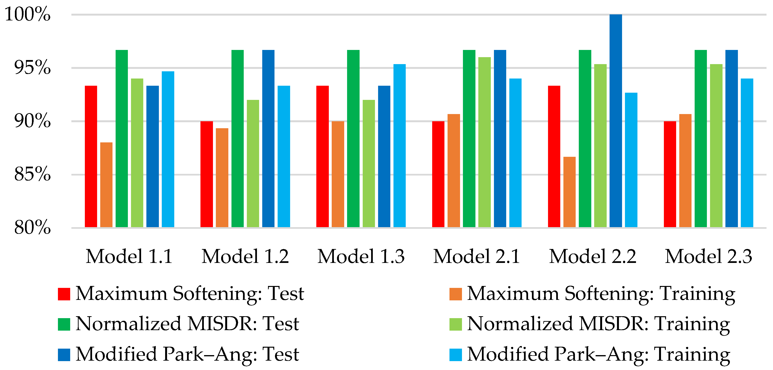
3.1. Training the Multiple Regression Models
3.2. Testing the Multiple Regression Models
3.3. Comparison of the Proposed Methodology with Predictions Obtained Through Compound IM
4. Conclusions
- Spectral-based and energy-related IMs correlated strongly with observed damage indices, reinforcing their relevance in damage assessment models;
- Velocity-based IMs, particularly Peak Ground Velocity (PGV) and Sustained Maximum Velocity, were also significant predictors;
- The multiple regression analysis confirmed that a limited set of IMs could effectively predict the structural damage grade, reducing the complexity of damage estimation without compromising accuracy and computational efficiency;
- The introduction of correlation-based weighting, in the form of exponentiation, enhanced prediction accuracy and damage grade classification;
- Both Forward Stepwise Selection-generated models presented the best overall performance regarding prediction accuracy and damage grade classification compared to their Ordinary Least Squares and Backward Stepwise Selection counterparts.
Author Contributions
Funding
Institutional Review Board Statement
Informed Consent Statement
Data Availability Statement
Conflicts of Interest
Abbreviations
| IM | Intensity Measure |
| DI | Damage Index |
| MISDR | Maximum Inter-Story Drift Ratio |
| NMISDR | Normalized Maximum Inter-Story Drift Ratio |
| SHM | Structural Health Monitoring |
| EDP | Engineering Demand Parameter |
References
- EN 1998-1:2004; Eurocode 8: Design of Structures for Earthquake Resistance—Part 1: General Rules, Seismic Actions and Rules for Buildings. CEN-CENELEC: Buffalo, NY, USA, 2004.
- EN 1992-1-1:2004; Eurocode 2: Design of Concrete Structures—Part 1-1: General Rules and Rules for Buildings. CEN-CENELEC: Brussels, Belgium, 2004.
- Kramer, S.L. Geotechnical Earthquake Engineering, 1 ed.; Prentice Hall, Inc.: Upper Saddle River, NJ, USA, 1996. [Google Scholar]
- Riddell, R. On Ground Motion Intensity Indices. Earthq. Spectra 2007, 23, 147–173. [Google Scholar] [CrossRef]
- Williams, M.S.; Sexsmith, R.G. Seismic Damage Indices for Concrete Structures: A State-of-the-Art Review. Earthq. Spectra 1995, 11, 319–349. [Google Scholar] [CrossRef]
- Kappos, A.J. Seismic damage indices for RC buildings: Evaluation of concepts and procedures. Prog. Struct. Eng. Mater. 1997, 1, 78–87. [Google Scholar] [CrossRef]
- Reinhorn, A.; Roh, H.; Sivaselvan, M.; Kunnath, S.; Valles, R.; Madan, A.; Li, C.; Lobo, R.; Park, Y. IDARC2D Version 7.0: A Program for the Inelastic Damage Analysis of Structures; MCEER-09-0006; Multidisciplinary Center for Earthquake Engineering Research: Buffalo, NY, USA, 2009. [Google Scholar]
- DiPasquale, E.; Cakmak, A.S. On the Relation Between Local and Global Damage Indices; NCEER-89-0034; National Center for Earthquake Engineering Research: Buffalo, NY, USA, 1989. [Google Scholar]
- Bhowmik, B.; Tripura, T.; Hazra, B.; Pakrashi, V. First-Order Eigen-Perturbation Techniques for Real-Time Damage Detection of Vibrating Systems: Theory and Applications. Appl. Mech. Rev. 2019, 71, 060801. [Google Scholar] [CrossRef]
- Chen, H.-P.; Bicanic, N. Inverse damage prediction in structures using nonlinear dynamic perturbation theory. Comput. Mech. 2005, 37, 455–467. [Google Scholar] [CrossRef]
- Xu, H.; Cheng, L.; Su, Z.; Guyader, J.-L. Damage visualization based on local dynamic perturbation: Theory and application to characterization of multi-damage in a plane structure. J. Sound Vib. 2013, 332, 3438–3462. [Google Scholar] [CrossRef]
- Xu, H.; Cheng, L.; Su, Z.; Guyader, J.-L. Identification of structural damage based on locally perturbed dynamic equilibrium with an application to beam component. J. Sound Vib. 2011, 330, 5963–5981. [Google Scholar] [CrossRef]
- Xu, W.; Zhu, W.; Su, Z.; Cao, M.; Xu, H. A novel structural damage identification approach using damage-induced perturbation in longitudinal vibration. J. Sound Vib. 2021, 496, 115932. [Google Scholar] [CrossRef]
- Cabañas, L.; Benito, B.; Herráiz, M. An Approach to the Measurement of the Potential Structural Damage of Earthquake Ground Motions. Earthq. Eng. Struct. Dyn. 1997, 26, 79–92. [Google Scholar] [CrossRef]
- Elenas, A.; Meskouris, K. Correlation study between seismic acceleration parameters and damage indices of structures. Eng. Struct. 2001, 23, 698–704. [Google Scholar] [CrossRef]
- Elenas, A. Seismic-Parameter-Based Statistical Procedures for the Approximate Assessment of Structural Damage. Math. Probl. Eng. 2014, 2014, 916820. [Google Scholar] [CrossRef]
- Cornell, C.A.; Jalayer, F.; Hamburger, R.O.; Foutch, D.A. Probabilistic Basis for 2000 SAC Federal Emergency Management Agency Steel Moment Frame Guidelines. J. Struct. Eng. 2002, 128, 526–533. [Google Scholar] [CrossRef]
- Liu, T.-T.; Lu, D.-G.; Yu, X.-H. Development of a compound intensity measure using partial least-squares regression and its statistical evaluation based on probabilistic seismic demand analysis. Soil Dyn. Earthq. Eng. 2019, 125, 105725. [Google Scholar] [CrossRef]
- Liu, T.-T.; Yu, X.-H.; Lu, D.-G. An Approach to Develop Compound Intensity Measures for Prediction of Damage Potential of Earthquake Records Using Canonical Correlation Analysis. J. Earthq. Eng. 2018, 24, 1747–1770. [Google Scholar] [CrossRef]
- Karampinis, I.; Bantilas, K.E.; Kavvadias, I.E.; Iliadis, L.; Elenas, A. Machine Learning Algorithms for the Prediction of the Seismic Response of Rigid Rocking Blocks. Appl. Sci. 2024, 14, 341. [Google Scholar]
- Lazaridis, P.C.; Kavvadias, I.E.; Demertzis, K.; Iliadis, L.; Vasiliadis, L.K. Structural Damage Prediction of a Reinforced Concrete Frame under Single and Multiple Seismic Events Using Machine Learning Algorithms. Appl. Sci. 2022, 12, 3845. [Google Scholar] [CrossRef]
- Liu, T.-T.; Lu, D.-G. Evaluation of Ground Motion Damage Potential with Consideration of Compound Intensity Measures Using Principal Component Analysis and Canonical Correlation Analysis. Buildings 2024, 14, 1309. [Google Scholar] [CrossRef]
- Xu, M.-Y.; Lu, D.-G.; Yu, X.-H.; Jia, M.-M. Selection of optimal seismic intensity measures using fuzzy-probabilistic seismic demand analysis and fuzzy multi-criteria decision approach. Soil Dyn. Earthq. Eng. 2023, 164, 107615. [Google Scholar] [CrossRef]
- Wang, X.; Qu, Z. A Computationally Efficient Algorithm for Constructing Effective Vector-Valued Seismic Intensity Measures for Engineering Structures. J. Earthq. Eng. 2024, 28, 3447–3468. [Google Scholar] [CrossRef]
- Montgomery, D.C.; Runger, G.C. Applied Statistics and Probability for Engineers, 7th ed.; John Siley & Sons: Hoboken, NJ, USA, 2018. [Google Scholar]
- Trifunac, M.D.; Brady, A.G. A study on the duration of strong earthquake ground motion. Bull. Seismol. Soc. Am. 1975, 65, 581–626. [Google Scholar] [CrossRef]
- Arias, A. Arias, A. A Measure of Earthquake Intensity. In Seismic Design for Nuclear Power Plants; Hansen, R.J., Ed.; Massachusetts Institute of Technology Press: Cambridge, MA, USA, 1970; pp. 438–483. [Google Scholar]
- SeismoSignal—A Computer Program for Signal Processing of Time-Histories; Seismosoft Ltd.: Pavia, Italy, 2024.
- Seyhan, E.; Stewart, J.P.; Ancheta, T.D.; Darragh, R.B.; Graves, R.W. NGA-West2 Site Database. Earthq. Spectra 2014, 30, 1007–1024. [Google Scholar] [CrossRef]
- Housner, G.W. Spectrum Intensities of Strong-Motion Earthquakes. In Proceedings of the Symposium on Earthquake and Blast Effects on Structures, Oakland, CA, USA, June 1952; pp. 20–36. [Google Scholar]
- Bianchini, M.; Diotallevi, P.P.; Baker, J.W. Prediction of inelastic structural response using an average of spectral accelerations. In Proceedings of the 10th International Conference on Structural Safety and Reliability (ICOSSAR09), Osaka, Japan, 13–17 September 2009; pp. 2164–2171. [Google Scholar]
- Sarma, S.K.; Yang, K.S. An evaluation of strong motion records and a new parameter A95. Earthq. Eng. Struct. Dyn. 1987, 15, 119–132. [Google Scholar] [CrossRef]
- Von Thun, J.L.; Scott, G.A.; Wilson, J.A. Earthquake ground motions for design and analysis of dams. In Proceedings of the Earthquake Engineering and Soil Dynamics II—Recent Advances in Ground-Motion Evaluation, Park City, UT, USA, 27–30 June 1988. [Google Scholar]
- Nuttli, O.W. State-of-the-Art for Assessing Earthquake Hazards in the United States. Report 16: The Relation of Sustained Maximum Ground Acceleration and Velocity to Earthquake Intensity and Magnitude; St. Louis University, Department of Earth and Atmospheric Sciences: St. Louis, MO, USA, 1979. [Google Scholar]
- Anderson, J.C.; Bertero, V.V. Uncertainties in Establishing Design Earthquakes. J. Struct. Eng. 1987, 113, 1709–1724. [Google Scholar] [CrossRef]
- Guamán, J.W. Empirical Ground Motion Relationships for Maximum Incremental Velocity. Ph.D. Thesis, University of Notre Dame, Notre Dame, Indiana, IN, USA, 2010. [Google Scholar]
- Newmark, N.M. A Study of Vertical and Horizontal Earthquake Spectra; Report WASH-1255; Unites States Atomic Energy Commission: Washington, DC, USA, 1973. [Google Scholar]
- Rathje, E.M.; Abrahamson, N.A.; Bray, J.D. Simplified Frequency Content Estimates of Earthquake Ground Motions. J. Geotech. Geoenviron. Eng. 1998, 124, 150–159. [Google Scholar] [CrossRef]
- Campbell, K.W.; Bozorgnia, Y. Prediction equations for the standardized version of cumulative absolute velocity as adapted for use in the shutdown of U.S. nuclear power plants. Nucl. Eng. Des. 2011, 241, 2558–2569. [Google Scholar] [CrossRef]
- Reed, J.W.; Kassawara, R.P. A criterion for determining exceedance of the operating basis earthquake. Nucl. Eng. Des. 1990, 123, 387–396. [Google Scholar] [CrossRef]
- Hanks, T.C. b values and ω−γ seismic source models: Implications for tectonic stress variations along active crustal fault zones and the estimation of high-frequency strong ground motion. J. Geophys. Res. Solid Earth 1979, 84, 2235–2242. [Google Scholar] [CrossRef]
- Manesh, M.R.; Saffari, H. Empirical equations for the prediction of the bracketed and uniform duration of earthquake ground motion using the Iran database. Soil Dyn. Earthq. Eng. 2020, 137, 106306. [Google Scholar] [CrossRef]
- Bolt, B.A. Duration of strong ground motion. In Proceedings of the 5th World Conference on Earthquake Engineering, Rome, Italy, 25–29 June 1973; pp. 1304–1313. [Google Scholar]
- Jennings, P.C. Engineering Seismology. In Earthquakes: Observation, Theory and Interpretation; Kanamori, H., Boschi, E., Eds.; Elsevier: Varenna, Italy, 1982. [Google Scholar]
- Malhotra, P.K. Cyclic-demand spectrum. Earthq. Eng. Struct. Dyn. 2002, 31, 1441–1457. [Google Scholar] [CrossRef]
- Hancock, J.; Bommer, J.J. The effective number of cycles of earthquake ground motion. Earthq. Eng. Struct. Dyn. 2005, 34, 637–664. [Google Scholar] [CrossRef]
- Panella, D.S.; Tornello, M.E.; Frau, C.D. A simple and intuitive procedure to identify pulse-like ground motions. Soil Dyn. Earthq. Eng. 2017, 94, 234–243. [Google Scholar] [CrossRef]
- Rodríguez-Gómez, S.; Cakmak, A.S. Evaluation of Seismic Damage Indices for Reinforced Concrete Structures; NCEER-90-0022; National Center for Earthquake Engineering Research: Buffalo, NY, USA, 1990. [Google Scholar]
- Stone, W.C.; Taylor, A.W. Seismic Performance of Circular Bridge Columns Designed in Accordance with AASHTO/CALTRANS Standards; National Institute of Standards and Technology: Gaithersburg, MD, USA, 1993. [Google Scholar]
- Gunturi, S.K.V.; Shah, H.C. Building specific damage estimation. In Proceedings of the 10th World Conference on Earthquake Engineering, Rotterdam, The Netherlands, 19–24 July 1992; pp. 6001–6006. [Google Scholar]
- Prestandard and Commentary for the Seismic Rehabilitation of Buildings American Society of Civil Engineers; Federal Emergency Management Agency: Washington, DC, USA, 2000.
- STAGRAPHICS Centurion XV User Manual; Statpoint Technologies Inc.: Warrenton, VA, USA, 2005.
| Damage Grade | MISDR | Modified Park–Ang | Maximum Softening |
|---|---|---|---|
| Minor | ≤0.5% | ≤0.30 | ≤0.30 |
| Moderate | 0.5–1.5% | 0.30–0.60 | 0.30–0.60 |
| Severe | 1.5–2.5% | 0.60–0.80 | 0.60–0.80 |
| Partial or Total Collapse | ≥2.5% | ≥0.80 | ≥0.80 |
| Model | Expression | Regression Method |
|---|---|---|
| Model 1.1 | Ordinary Least Squares | |
| Model 1.2 | Forward Stepwise Selection | |
| Model 1.3 | Backward Stepwise Selection | |
| Model 2.1 1 | Ordinary Least Squares | |
| Model 2.2 1 | Forward Stepwise Selection | |
| Model 2.3 1 | Backward Stepwise Selection |
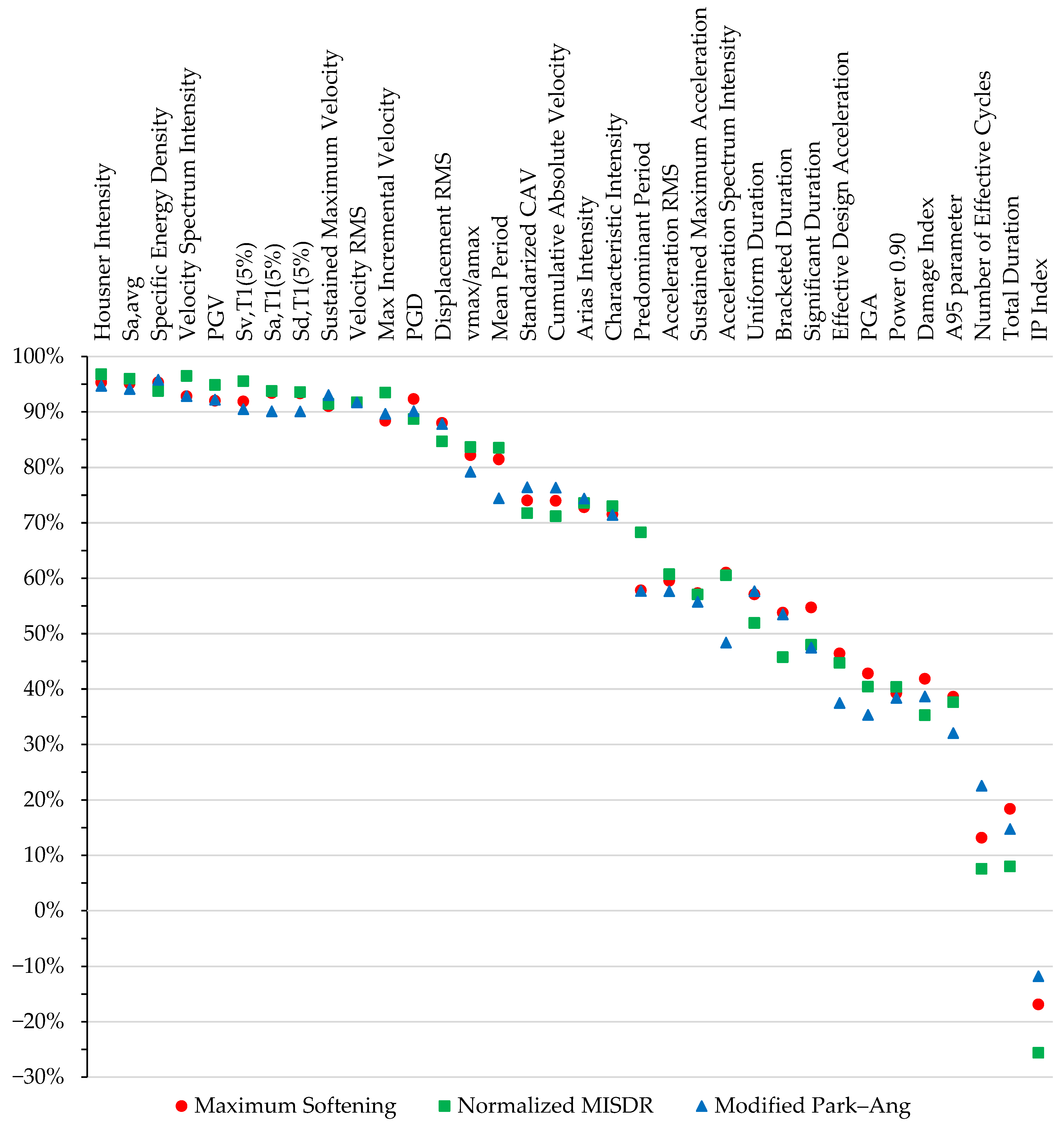
| Intensity Measure | Normalized MISDR | Maximum Softening | Modified Park–Ang |
|---|---|---|---|
| Housner Intensity | 96.79% | 95.32% | 94.71% |
| Sa,avg | 95.98% | 95.12% | 94.12% |
| Specific Energy Density | 93.75% | 95.31% | 95.79% |
| Velocity Spectrum Intensity | 96.47% | 92.81% | 92.84% |
| PGV | 94.85% | 92.00% | 92.20% |
| Sv,T1(5%) | 95.54% | 91.88% | 90.49% |
| Sa,T1(5%) | 93.76% | 93.38% | 90.09% |
| Sd,T1(5%) | 93.57% | 93.32% | 90.07% |
| Sustained Maximum Velocity | 91.43% | 91.01% | 93.03% |
| Velocity RMS | 91.72% | 91.73% | 91.69% |
| Intensity Measure | Model 1.1 | Model 1.2 | Model 1.3 | Model 2.1 | Model 2.2 | Model 2.3 |
|---|---|---|---|---|---|---|
| Housner Intensity | −0.00315 | −0.00396 | −0.00327 | −0.03584 | −0.03541 | −0.03617 |
| Sa,avg | 2.14631 | 2.27422 | 2.09444 | 1.61169 | 2.01052 | 1.60807 |
| Specific Energy Density | −3.55 × 10⁻⁷ | - | - | 0.00082 | 0.00079 | 0.00088 |
| Velocity Spectrum Intensity | −0.00046 | - | - | −0.02279 | −0.06588 | - |
| PGV | 0.00101 | 0.00147 | - | 0.06651 | - | - |
| Sv,T1(5%) | 0.00207 | - | 0.00172 | −0.03221 | - | - |
| Sa,T1(5%) | 1.28091 | - | - | −9.87011 | - | −9.96924 |
| Sd,T1(5%) | −0.04399 | - | −0.00987 | 3.02685 | - | 3.03894 |
| Sustained Maximum Velocity | 0.00210 | 0.00317 | 0.00214 | −0.36318 | - | −0.36436 |
| Velocity RMS | 0.00644 | - | 0.00881 | 0.18342 | - | 0.19688 |
| Intensity Measure | Model 1.1 | Model 1.2 | Model 1.3 | Model 2.1 | Model 2.2 | Model 2.3 |
|---|---|---|---|---|---|---|
| Housner Intensity | −0.00233 | −0.00388 | −0.00277 | −0.01671 | - | - |
| Sa,avg | 2.56422 | 2.43042 | 2.45724 | 1.66802 | 1.18412 | 1.18412 |
| Specific Energy Density | 0.00000 | 4.30 × 10⁻⁶ | 3.91× 10⁻⁶ | 0.00925 | 0.00826 | 0.00826 |
| Velocity Spectrum Intensity | −0.00133 | 0.00119 | - | 0.00560 | - | - |
| PGV | 0.00100 | - | - | 0.01069 | - | - |
| Sv,T1(5%) | 0.00361 | - | 0.00226 | 0.00840 | - | - |
| Sa,T1(5%) | 11.08590 | - | - | 2.94016 | - | - |
| Sd,T1(5%) | −0.30221 | - | −0.01104 | −0.81300 | - | - |
| Sustained Maximum Velocity | 0.00011 | - | - | −0.26576 | −0.14961 | −0.14961 |
| Velocity RMS | 0.00282 | - | - | 0.12614 | - | - |
| Intensity Measure | Model 1.1 | Model 1.2 | Model 1.3 | Model 2.1 | Model 2.2 | Model 2.3 |
|---|---|---|---|---|---|---|
| Housner Intensity | 0.00084 | - | - | 0.06351 | 0.04842 | 0.07174 |
| Sa,avg | 0.84262 | 0.48282 | 1.09999 | 0.29184 | - | - |
| Specific Energy Density | 0.00001 | 0.00001 | 0.00001 | 0.00119 | 0.00136 | 0.00129 |
| Velocity Spectrum Intensity | −0.00196 | - | −0.00180 | −0.28076 | −0.08295 | −0.20725 |
| PGV | 0.00014 | - | - | 0.08743 | - | - |
| Sv,T1(5%) | 0.00330 | - | 0.00277 | 3.16888 | - | 2.70311 |
| Sa,T1(5%) | −11.95520 | - | −0.36320 | −51.95980 | - | −45.04080 |
| Sd,T1(5%) | 0.29622 | - | - | 46.97820 | - | 40.80560 |
| Sustained Maximum Velocity | 0.00199 | 0.00207 | 0.00212 | 0.02463 | - | - |
| Velocity RMS | 0.00099 | - | - | −0.04007 | - | - |
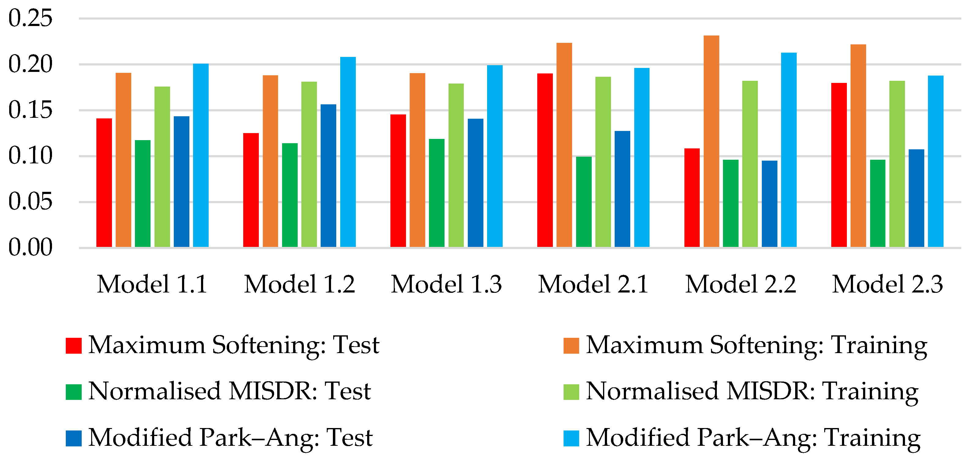
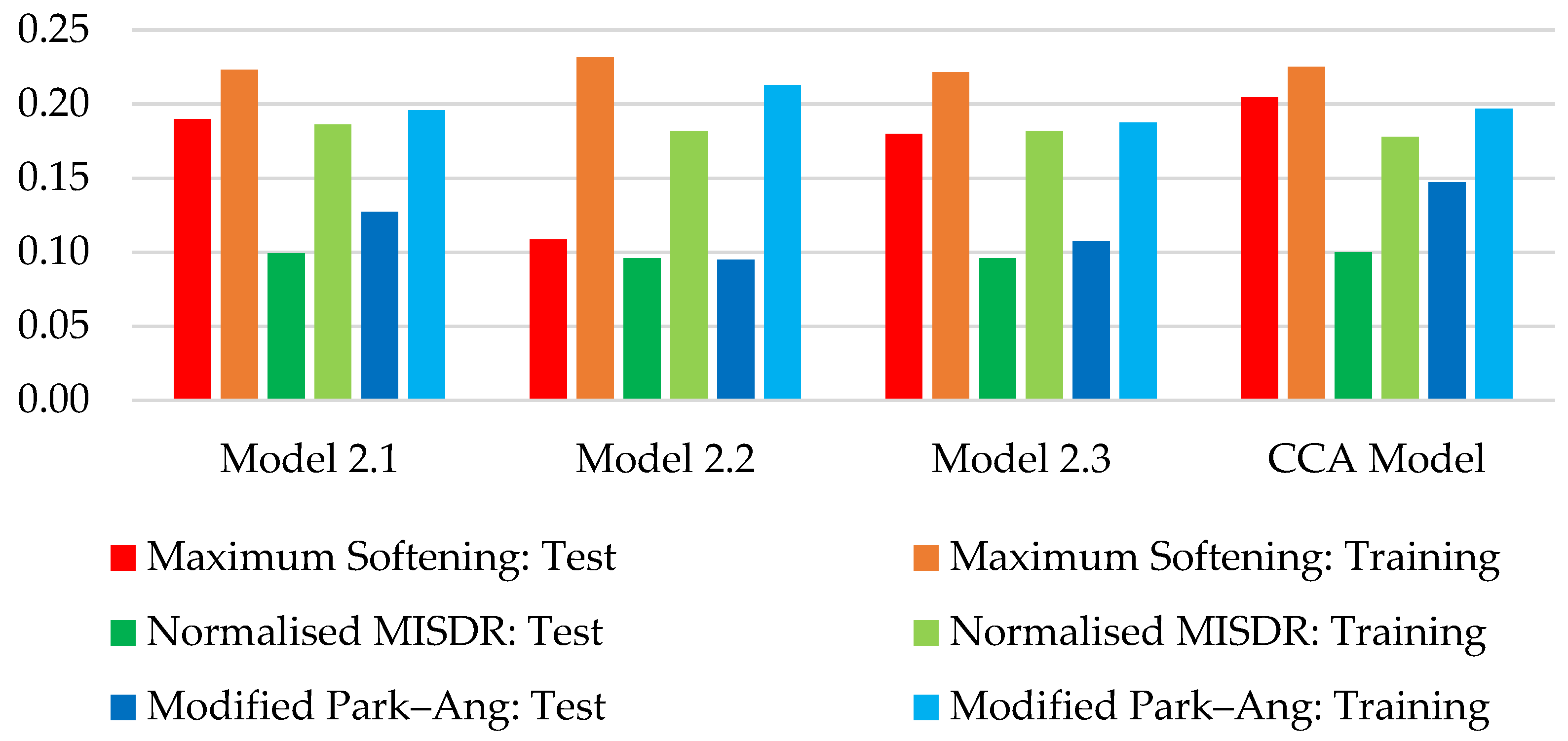
| Model | RMSE Normalized MISDR | RMSE Maximum Softening | RMSE Modified Park–Ang | Adjusted–R2 Normalized MISDR | Adjusted–R2 Maximum Softening | Adjusted–R2 Modified Park–Ang |
|---|---|---|---|---|---|---|
| Model 1.1 | 0.1429 | 0.1191 | 0.1080 | 94.97% | 94.04% | 94.00% |
| Model 2.1 | 0.1223 | 0.0771 | 0.1018 | 96.31% | 97.50% | 94.66% |
| Model 1.2 | 0.1433 | 0.1197 | 0.1121 | 94.94% | 93.97% | 93.52% |
| Model 2.2 | 0.1225 | 0.0804 | 0.1027 | 96.30% | 97.28% | 94.57% |
| Model 1.3 | 0.1419 | 0.1181 | 0.1077 | 95.03% | 94.13% | 94.03% |
| Model 2.3 | 0.1225 | 0.0765 | 0.1011 | 96.30% | 97.54% | 94.74% |
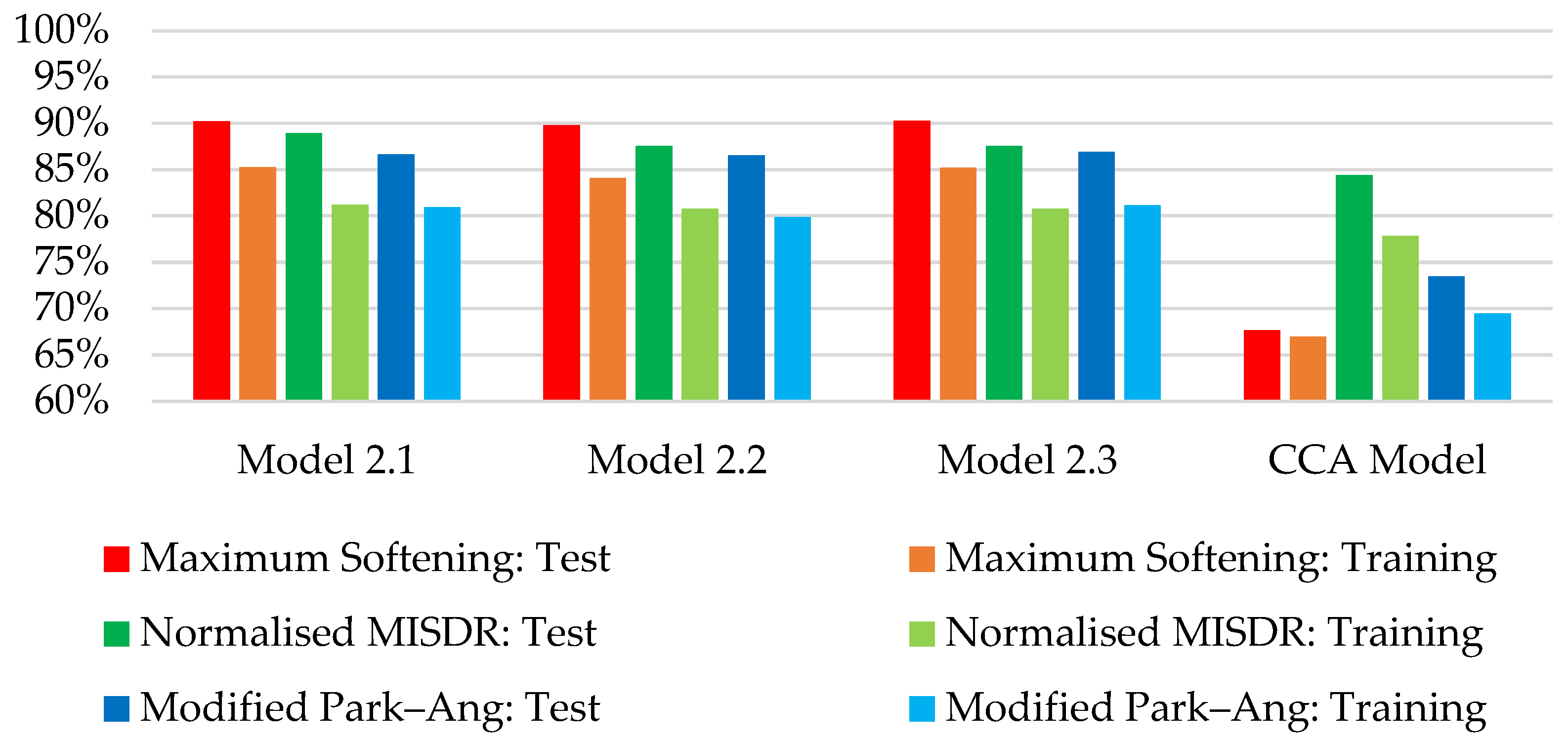
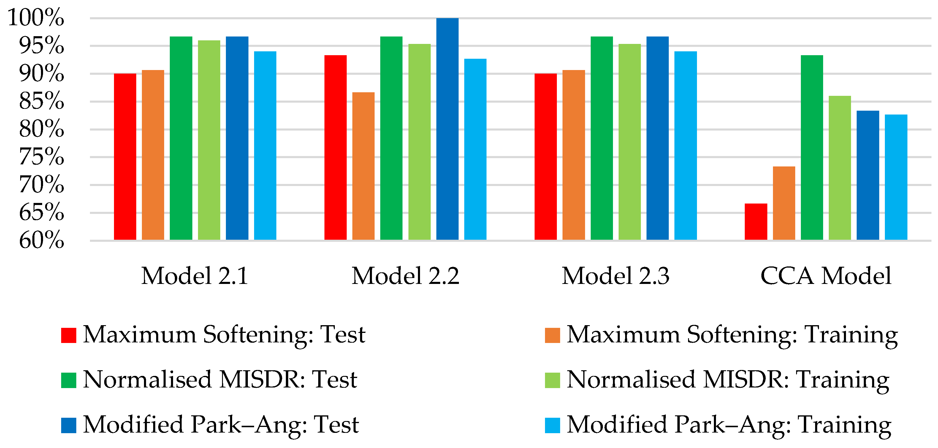
| Model | Average Prediction Accuracy: Test Set | Average Prediction Accuracy: Training Set | Average of Success Rate of Correctly Identified Damage Grade: Test Set | Average of Success Rate of Correctly Identified Damage Grade: Training Set | Average Prediction Accuracy: Test and Training Sets | Average of Success Rate of Correctly Identified Damage Grade: Test and Training Sets |
|---|---|---|---|---|---|---|
| Model 1.1 | 83.05% | 78.73% | 94.44% | 92.22% | 80.89% | 93.33% |
| Model 2.1 | 88.59% | 82.46% | 94.44% | 93.56% | 85.53% | 94.00% |
| Model 1.2 | 84.06% | 78.39% | 94.44% | 91.56% | 81.22% | 93.00% |
| Model 2.2 | 87.97% | 81.58% | 96.67% | 91.56% | 84.77% | 94.11% |
| Model 1.3 | 83.01% | 78.81% | 94.44% | 92.44% | 80.91% | 93.44% |
| Model 2.3 | 88.26% | 82.37% | 94.44% | 93.33% | 85.32% | 93.89% |
Disclaimer/Publisher’s Note: The statements, opinions and data contained in all publications are solely those of the individual author(s) and contributor(s) and not of MDPI and/or the editor(s). MDPI and/or the editor(s) disclaim responsibility for any injury to people or property resulting from any ideas, methods, instructions or products referred to in the content. |
© 2025 by the authors. Licensee MDPI, Basel, Switzerland. This article is an open access article distributed under the terms and conditions of the Creative Commons Attribution (CC BY) license (https://creativecommons.org/licenses/by/4.0/).
Share and Cite
Chaitas, E.; Kavvadias, I.E.; Bantilas, K.E.; Elenas, A. An Alternative Procedure for the Description of Seismic Intensity Parameter-Based Damage Potential. Appl. Sci. 2025, 15, 3949. https://doi.org/10.3390/app15073949
Chaitas E, Kavvadias IE, Bantilas KE, Elenas A. An Alternative Procedure for the Description of Seismic Intensity Parameter-Based Damage Potential. Applied Sciences. 2025; 15(7):3949. https://doi.org/10.3390/app15073949
Chicago/Turabian StyleChaitas, Emmanouil, Ioannis E. Kavvadias, Kosmas E. Bantilas, and Anaxagoras Elenas. 2025. "An Alternative Procedure for the Description of Seismic Intensity Parameter-Based Damage Potential" Applied Sciences 15, no. 7: 3949. https://doi.org/10.3390/app15073949
APA StyleChaitas, E., Kavvadias, I. E., Bantilas, K. E., & Elenas, A. (2025). An Alternative Procedure for the Description of Seismic Intensity Parameter-Based Damage Potential. Applied Sciences, 15(7), 3949. https://doi.org/10.3390/app15073949