
Urban Green Space Inequity, Socioeconomic Disparities, and Potential Health Implications in Metropolitan Melbourne


Abstract
1. Introduction
2. Methods
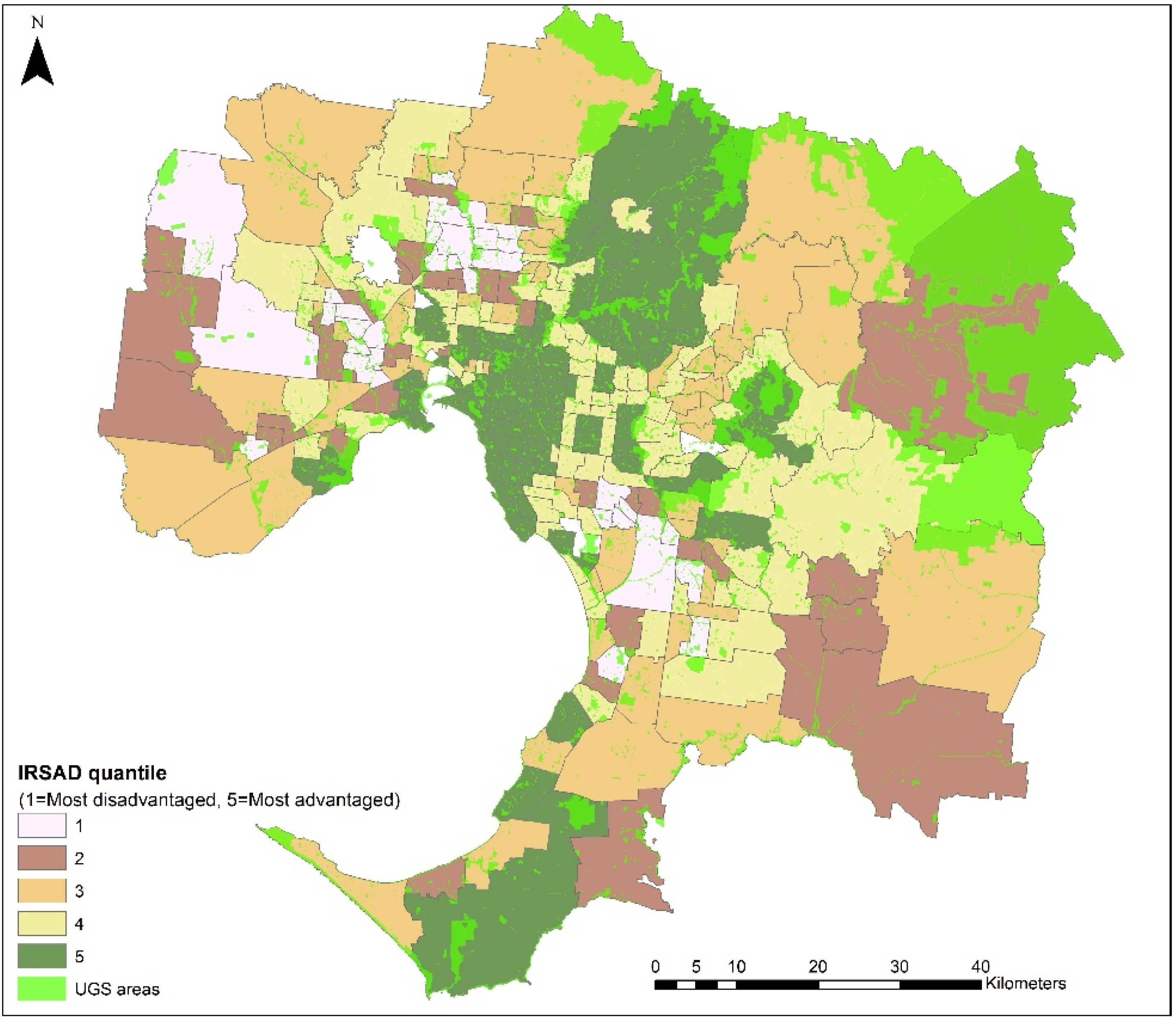
2.1. Study Area
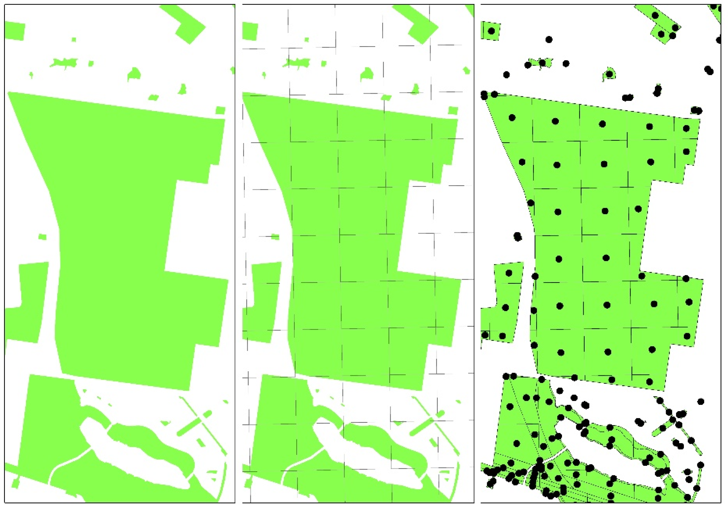
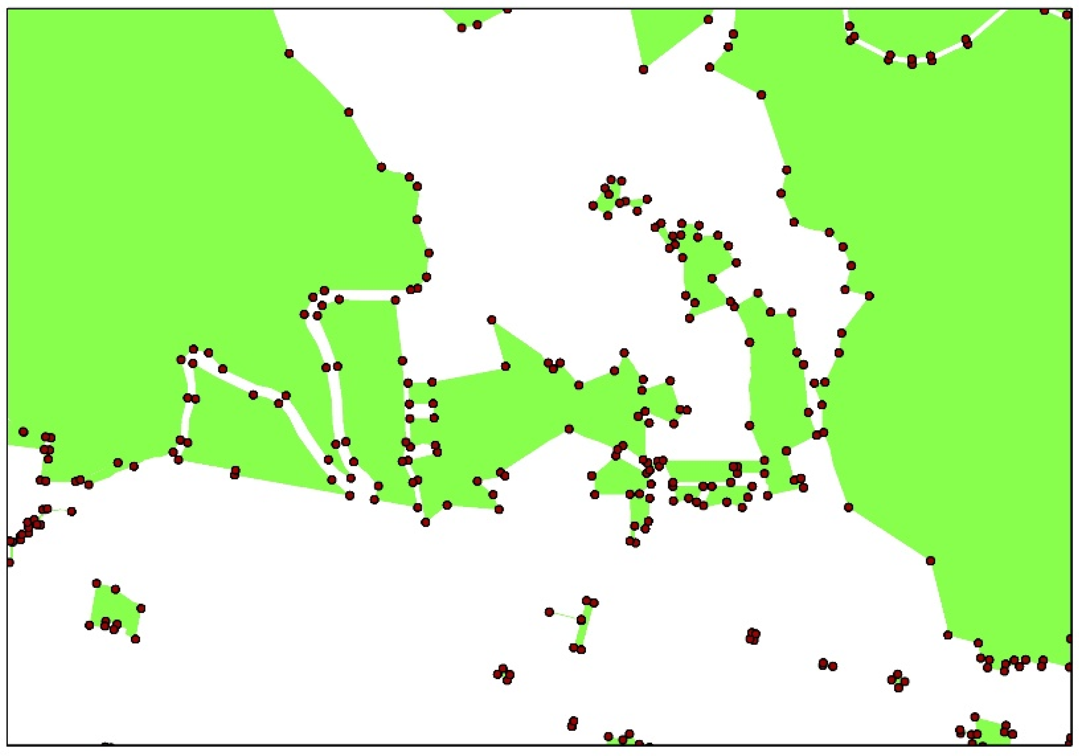
2.2. Urban Green Space Data
- Have vegetation or green space area to provide a chance for contact with nature;
- Open for public use without charge or membership;
- Devoted to, or amenable to, recreational purposes.
- Conservation reserves;
- Natural and semi-natural open space;
- Parks and gardens;
- Sports fields.
- UGS density;
- Accessibility;
- Provision.
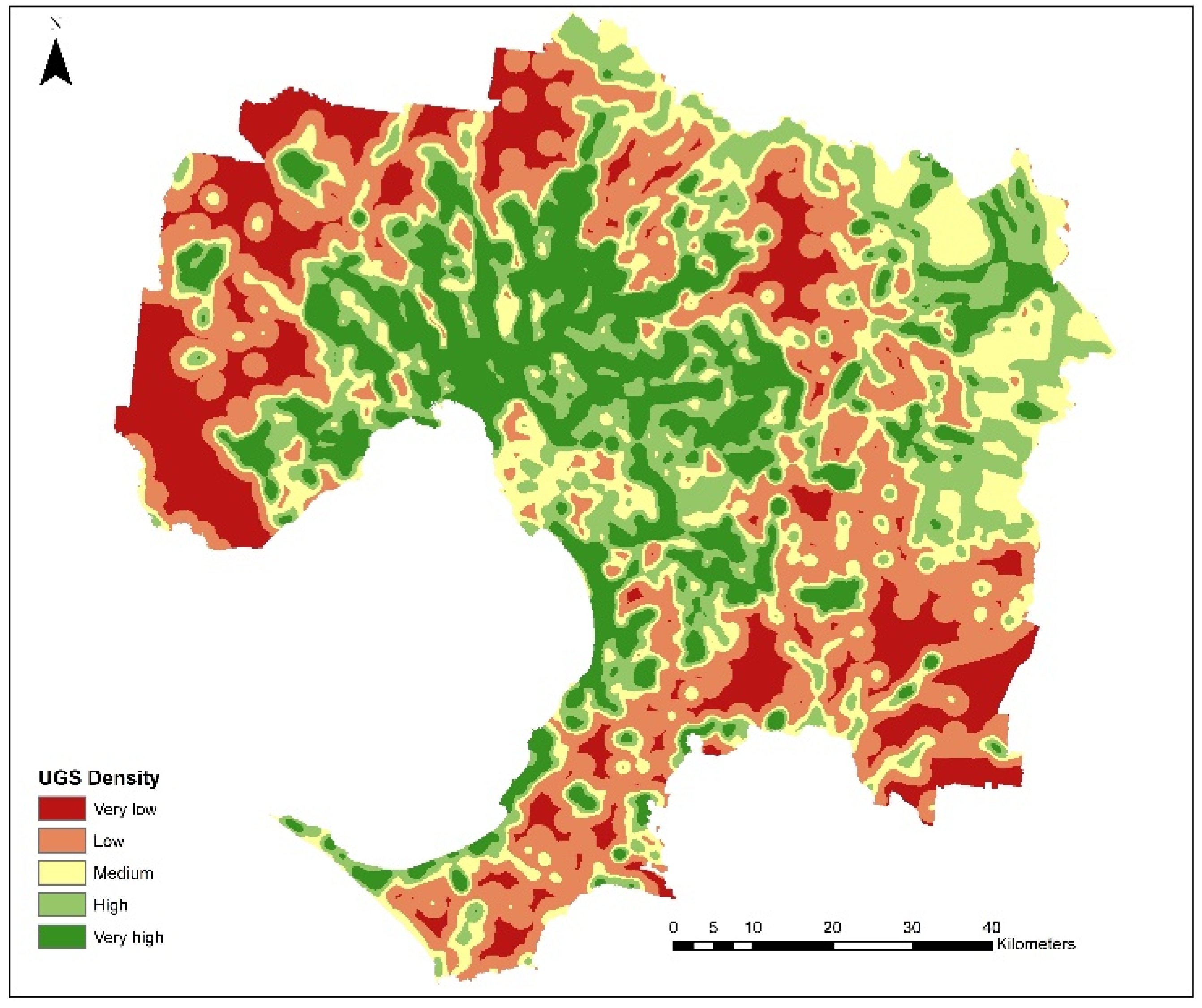
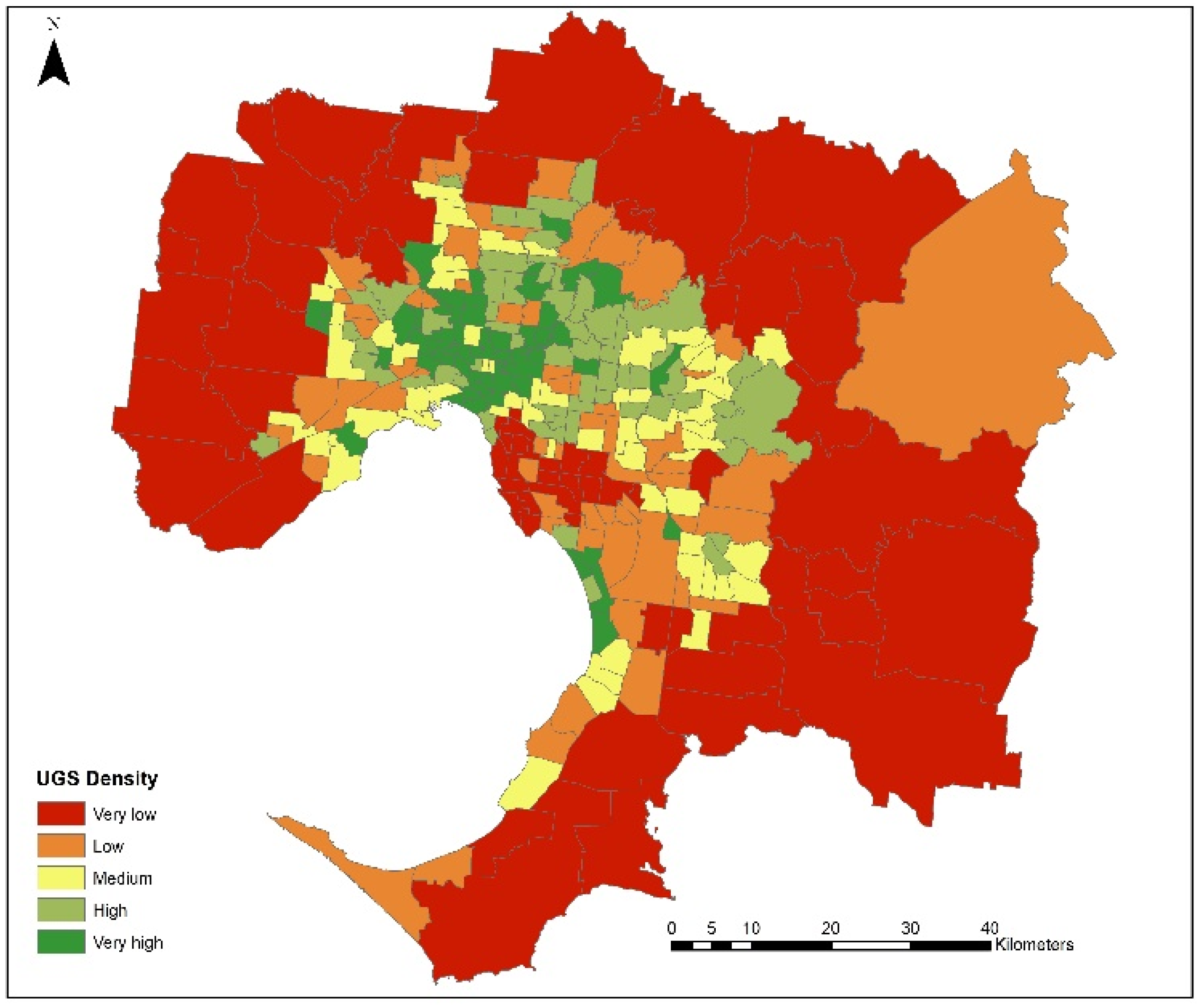
2.3. UGS Density
Accessibility and Provision
2.4. SES Data
2.5. Health Data
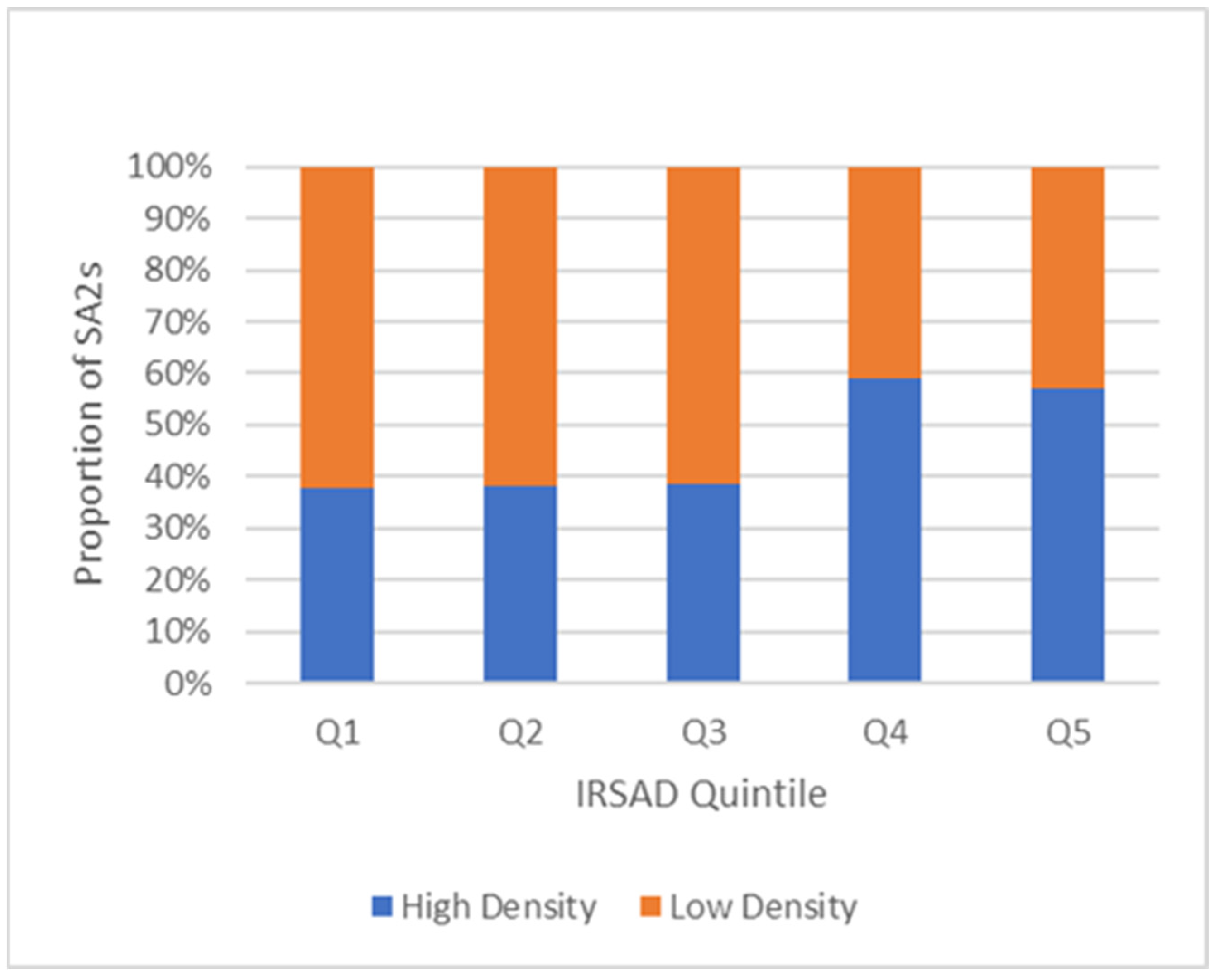
2.6. Data Analysis
- High Access—High Density Areas;
- High Access—Low Density Areas;
- Low Access—High Density Areas;
- Low Access—Low Density Areas.
3. Results
4. Discussion
5. Conclusions
Author Contributions
Funding
Data Availability Statement
Acknowledgments
Conflicts of Interest
References
- Giles-Corti, B.; Saghapour, T.; Turrell, G.; Gunn, L.; Both, A.; Lowe, M.; Rozek, J.; Roberts, R.; Hooper, P.; Butt, A.; et al. Spatial and socioeconomic inequities in liveability in Australia’s 21 largest cities: Does city size matter? Health Place 2022, 78, 102899. [Google Scholar] [CrossRef]
- Leng, H.; Li, S.; Yan, S.; An, X. Exploring the relationship between green space in a neighbourhood and cardiovascular health in the winter city of China: A study using a health survey for harbin. Int. J. Environ. Res. Public Health 2020, 17, 513. [Google Scholar] [CrossRef]
- Browning, M.; Lee, K. Within what distance does “greenness” best predict physical health? A systematic review of articles with gis buffer analyses across the lifespan. Int. J. Environ. Res. Public Health 2017, 14, 675. [Google Scholar] [CrossRef]
- Schindler, M.; Le Texier, M.; Caruso, G. How far do people travel to use urban green space? A comparison of three European cities. Appl. Geogr. 2022, 141, 102673. [Google Scholar]
- Sullivan, W.C.; Kuo, F.E.; Depooter, S.F. The fruit of urban nature: Vital neighborhood spaces. Environ. Behav. 2004, 36, 678–700. [Google Scholar]
- Zhang, R.; Zhang, C.-Q.; Cheng, W.; Lai, P.C.; Schüz, B. The neighborhood socioeconomic inequalities in urban parks in a High-density City: An environmental justice perspective. Landsc. Urban Plan. 2021, 211, 104099. [Google Scholar] [CrossRef]
- Richardson, E.; Pearce, J.; Mitchell, R.; Kingham, S. Role of physical activity in the relationship between urban green space and health. Public Health 2013, 127, 318–324. [Google Scholar] [CrossRef]
- Wood, L.; Hooper, P.; Foster, S.; Bull, F. Public green spaces and positive mental health—Investigating the relationship between access, quantity and types of parks and mental wellbeing. Health Place 2017, 48, 63–71. [Google Scholar] [CrossRef]
- Hoffimann, E.; Barros, H.; Ribeiro, A.I. Socioeconomic inequalities in green space quality and Accessibility—Evidence from a Southern European city. Int. J. Environ. Res. Public Health 2017, 14, 916. [Google Scholar] [CrossRef]
- Feng, X.; Astell-Burt, T.; Standl, M.; Flexeder, C.; Heinrich, J.; Markevych, I. Green space quality and adolescent mental health: Do personality traits matter? Environ. Res. 2022, 206, 112591. [Google Scholar] [CrossRef]
- Ghanem, A.; Edirisinghe, R. Socio-economic disparities in greenspace quality: Insights from the city of Melbourne. Smart Sustain. Built Environ. 2024, 13, 309–329. [Google Scholar]
- Selmi, W.; Weber, C.; Rivière, E.; Blond, N.; Mehdi, L.; Nowak, D. Air pollution removal by trees in public green spaces in Strasbourg city, France. Urban For. Urban Green. 2016, 17, 192–201. [Google Scholar]
- Taylor, L.; Hochuli, D.F. Defining greenspace: Multiple uses across multiple disciplines. Landsc. Urban Plan. 2017, 158, 25–38. [Google Scholar] [CrossRef]
- Yu, W.; Ai, T.; Shao, S. The analysis and delimitation of Central Business District using network kernel density estimation. J. Transp. Geogr. 2015, 45, 32–47. [Google Scholar] [CrossRef]
- Astell-Burt, T.; Feng, X. Urban green space, tree canopy and prevention of cardiometabolic diseases: A multilevel longitudinal study of 46 786 Australians. Int. J. Epidemiol. 2020, 49, 926–933. [Google Scholar] [CrossRef]
- Park, Y.M.; Kwan, M.-P. Multi-contextual segregation and environmental justice research: Toward fine-scale spatiotemporal approaches. Int. J. Environ. Res. Public Health 2017, 14, 1205. [Google Scholar] [CrossRef]
- Sharifi, F.; Nygaard, A.; Stone, W.M. Heterogeneity in the Subjective Well-being Impact of Access to Urban Green Space. Sustain. Cities Soc. 2021, 74, 103244. [Google Scholar] [CrossRef]
- Zhang, L.; Tan, P.Y.; Richards, D. Relative importance of quantitative and qualitative aspects of urban green spaces in promoting health. Landsc. Urban Plan. 2021, 213, 104131. [Google Scholar] [CrossRef]
- Raza, W.; Bojke, L.; Coventry, P.A.; Murphy, P.J.; Fulbright, H.; White, P.C. A Systematic Review of the Impact of Changes to Urban Green Spaces on Health and Education Outcomes, and a Critique of Their Applicability to Inform Economic Evaluation. Int. J. Environ. Res. Public Health 2024, 21, 1452. [Google Scholar] [CrossRef]
- Astell-Burt, T.; Navakatikyan, M.A.; Feng, X. Urban green space, tree canopy and 11 year risk of dementia in a cohort of 109,688 Australians. Environ. Int. 2020, 145, 106102. [Google Scholar]
- Maroko, A.R.; Maantay, J.A.; Sohler, N.L.; Grady, K.L.; Arno, P.S. The complexities of measuring access to parks and physical activity sites in New York City: A quantitative and qualitative approach. Int. J. Health Geogr. 2009, 8, 34. [Google Scholar] [CrossRef]
- Astell-Burt, T.; Feng, X.; Mavoa, S.; Badland, H.M.; Giles-Corti, B. Do low-income neighbourhoods have the least green space? A cross-sectional study of Australia’s most populous cities. BMC Public Health 2014, 14, 292. [Google Scholar] [CrossRef] [PubMed]
- Shuvo, F.K.; Feng, X.; Akaraci, S.; Astell-Burt, T. Urban green space and health in low and middle-income countries: A critical review. Urban For. Urban Green. 2020, 52, 126662. [Google Scholar] [CrossRef]
- Kabisch, N.; van den Bosch, M.; Lafortezza, R. The health benefits of nature-based solutions to urbanization challenges for children and the elderly—A systematic review. Environ. Res. 2017, 159, 362–373. [Google Scholar] [CrossRef] [PubMed]
- Kabisch, N.; Haase, D. Green justice or just green? Provision of urban green spaces in Berlin, Germany. Landsc. Urban Plan. 2014, 122, 129–139. [Google Scholar] [CrossRef]
- Pereira, G.; Foster, S.; Martin, K.; Christian, H.; Boruff, B.J.; Knuiman, M.; Giles-Corti, B. The association between neighborhood greenness and cardiovascular disease: An observational study. BMC Public Health 2012, 12, 466. [Google Scholar] [CrossRef] [PubMed]
- National Health Survey. Available online: https://www.abs.gov.au/statistics/health/health-conditions-and-risks/national-health-survey-first-results/2017-18 (accessed on 20 July 2021).
- Australian Health Expenditure—Demographics and Diseases: Hospital Admitted Patient Expenditure 2004-05 to 2012-13. Available online: https://www.aihw.gov.au/reports/health-welfare-expenditure/health-expenditure-australia-2017-18/contents/summary (accessed on 18 March 2025).
- Liu, X.X.; Ma, X.L.; Huang, W.Z.; Luo, Y.N.; He, C.J.; Zhong, X.M.; Dadvand, P.; Browning, M.H.; Li, L.; Zou, X.G.; et al. Green space and cardiovascular disease: A systematic review with meta-analysis. Environ. Pollut. 2022, 15, 118990. [Google Scholar] [CrossRef]
- Sandifer, P.A.; Sutton-Grier, A.E.; Ward, B.P. Exploring connections among nature, biodiversity, ecosystem services, and human health and well-being: Opportunities to enhance health and biodiversity conservation. Ecosyst. Serv. 2015, 12, 1–15. [Google Scholar] [CrossRef]
- Sharifi, F.; Nygaard, A.; Stone, W.M.; Levin, I. Green gentrification or gentrified greening: Metropolitan Melbourne. Land Use Policy 2021, 108, 105577. [Google Scholar] [CrossRef]
- Wolch, J.R.; Byrne, J.; Newell, J.P. Urban green space, public health, and environmental justice: The challenge of making cities “just green enough”. Landsc. Urban Plan. 2014, 125, 234–244. [Google Scholar] [CrossRef]
- Australian Statistical Geography Standard (ASGS). Available online: https://www.abs.gov.au/ausstats/abs@.nsf/lookup/by subject/1270.0.55.001~july 2016~main features~statistical area level 2 (sa2)~10014 (accessed on 20 July 2021).
- The 2016 Census of Population and Housing. Available online: https://www.abs.gov.au/%0Aausstats/abs@.nsf/Lookup/by (accessed on 15 July 2021).
- 68% of the World Population Projected to Live in Urban Areas by 2050. Available online: https://www.un.org/development/desa/en/news/population/2018-revision-of-world-urbanization-prospects.html (accessed on 18 March 2025).
- Wang, D.; Brown, G.; Liu, Y. The physical and non-physical factors that influence perceived access to urban parks. Landsc. Urban Plan. 2015, 133, 53–66. [Google Scholar] [CrossRef]
- VPA Open Data. Available online: https://data-planvic.opendata.arcgis.com/ (accessed on 18 March 2025).
- Boulton, C.; Dedekorkut-Howes, A.; Byrne, J. Factors shaping urban greenspace provision: A systematic review of the literature. Landsc. Urban Plan. 2018, 178, 82–101. [Google Scholar] [CrossRef]
- Chen, Z.; Sarkar, A.; Rahman, A.; Li, X.; Xia, X. Exploring the drivers of green agricultural development (GAD) in China: A spatial association network structure approaches. Land Use Policy 2022, 112, 105827. [Google Scholar]
- Kaplan, R. The nature of the view from home: Psychological benefits. Environ. Behav. 2001, 33, 507–542. [Google Scholar] [CrossRef]
- Point Density (Spatial Analysis). Available online: https://www.esri.com/en-us/arcgis/products/arcgis-pro/resources (accessed on 10 November 2021).
- Mavoa, S.; Koohsari, M.J.; Badland, H.M.; Davern, M.; Feng, X.; Astell-Burt, T.; Giles-Corti, B. Area-Level Disparities of Public Open Space: A Geographic Information Systems Analysis in Metropolitan Melbourne. Urban Policy Res. 2014, 33, 306–323. [Google Scholar] [CrossRef]
- de Sousa Silva, C.; Viegas, I.; Panagopoulos, T.; Bell, S. Environmental justice in accessibility to green infrastructure in two European Cities. Land 2018, 7, 134. [Google Scholar] [CrossRef]
- De Vries, S.; Verheij, R.A.; Groenewegen, P.P.; Spreeuwenberg, P. Natural environments—Healthy environments? An exploratory analysis of the relationship between greenspace and health. Environ. Plan. A 2003, 35, 1717–1731. [Google Scholar] [CrossRef]
- Victoria Planning Authority, Metropolitan Open Space Network, Map Journal. Available online: https://planvic.maps.arcgis.com/apps/MapJournal/index.html?appid=8965d9701575408e8ea7f59772e82e10 (accessed on 21 August 2022).
- Mytton, O.T.; Townsend, N.; Rutter, H.; Foster, C. Green space and physical activity: An observational study using Health Survey for England data. Health Place 2012, 18, 1034–1041. [Google Scholar] [CrossRef]
- Australian Bureau of Statistics, Socio-Economic Indexes for Areas. Census of Population and Housing 2016. Available online: https://www.abs.gov.au/AUSSTATS/abs@.nsf/DetailsPage/2033.0.55.0012016?OpenDocument (accessed on 20 July 2021).
- Lin, B.; Meyers, J.; Barnett, G. Understanding the potential loss and inequities of green space distribution with urban densification. Urban For. Urban Green. 2015, 14, 952–958. [Google Scholar] [CrossRef]
- Bilal, U.; Auchincloss, A.H.; Diez-Roux, A.V. Neighborhood Environments and Diabetes Risk and Control. Curr. Diabetes Rep. 2018, 18, 62. [Google Scholar] [CrossRef]
- Giles-Corti, B.; Moudon, A.V.; Lowe, M.; Cerin, E.; Boeing, G.; Frumkin, H.; Salvo, D.; Foster, S.; Kleeman, A.; Bekessy, S.; et al. What next? Expanding our view of city planning and global health, and implementing and monitoring evidence-informed policy. Lancet Glob. Health 2022, 10, e919–e926. [Google Scholar] [PubMed]


| Variable | N | Mean | Min | Max |
|---|---|---|---|---|
| UGS: | ||||
| Area (Ha) | 294 | 3166 | 148.87 | 86,417.26 |
| Per capita (m2) | 294 | 427.28 | 0.40 | 29,036.15 |
| Diseases (% of Total Pop) | 294 | 4.43 | 1.40 | 7.80 |
| IRSAD Score | 294 | 1028.62 | 819.00 | 1160.00 |
| Variable | N | DF | X2 | p-Value * |
|---|---|---|---|---|
| UGS: | ||||
| Access | 294 | 4 | 17.302 | 0.002 |
| Density | 294 | 4 | 11.105 | 0.025 |
| Per capita | 294 | 4 | 5.210 | 0.266 |
| Variable: | UGS Access | ||
|---|---|---|---|
| CVD (%) | Low | Mean | 4.56 |
| Std. Dev. | 1.17 | ||
| Min | 2.20 | ||
| Max | 7.80 | ||
| High | Mean | 4.30 | |
| Std. Dev. | 1.03 | ||
| Min | 1.40 | ||
| Max | 6.90 |
| Variable: | UGS Density | ||
|---|---|---|---|
| CVD (%) | Low | Mean | 4.60 |
| Std. Dev. | 1.13 | ||
| Min | 2.20 | ||
| Max | 7.80 | ||
| High | Mean | 4.26 | |
| Std. Dev. | 1.06 | ||
| Min | 1.40 | ||
| Max | 7.00 |
| UGS Availability | N | IRSAD Mean | Std. Dev. | Min | Max |
|---|---|---|---|---|---|
| High Access—High Density | 104 | 1054.29 | 58.61 | 920.00 | 1160.00 |
| High Access—Low Density | 43 | 1021.19 | 83.02 | 862.00 | 1147.00 |
| Low Access—High Density | 43 | 1010.19 | 67.92 | 846.00 | 1115.00 |
| Low Access—Low Density | 104 | 1013.64 | 66.91 | 819.00 | 1144.00 |
| UGS Availability | N | Disease Mean | Std. Dev. | Min | Max |
|---|---|---|---|---|---|
| High Access—High Density | 104 | 4.13 | 0.105 | 1.40 | 6.90 |
| High Access—Low Density | 43 | 4.71 | 0.117 | 2.80 | 6.60 |
| Low Access—High Density | 43 | 4.56 | 0.148 | 2.60 | 7.00 |
| Low Access—Low Density | 104 | 4.43 | 0.122 | 2.20 | 7.80 |
Disclaimer/Publisher’s Note: The statements, opinions and data contained in all publications are solely those of the individual author(s) and contributor(s) and not of MDPI and/or the editor(s). MDPI and/or the editor(s) disclaim responsibility for any injury to people or property resulting from any ideas, methods, instructions or products referred to in the content. |
© 2025 by the authors. Licensee MDPI, Basel, Switzerland. This article is an open access article distributed under the terms and conditions of the Creative Commons Attribution (CC BY) license (https://creativecommons.org/licenses/by/4.0/).
Share and Cite
Hoseini, P.; Mohseni, P.; Veeroja, P.; Foliente, G. Urban Green Space Inequity, Socioeconomic Disparities, and Potential Health Implications in Metropolitan Melbourne. Appl. Sci. 2025, 15, 3940. https://doi.org/10.3390/app15073940
Hoseini P, Mohseni P, Veeroja P, Foliente G. Urban Green Space Inequity, Socioeconomic Disparities, and Potential Health Implications in Metropolitan Melbourne. Applied Sciences. 2025; 15(7):3940. https://doi.org/10.3390/app15073940
Chicago/Turabian StyleHoseini, Parian, Pooriya Mohseni, Piret Veeroja, and Greg Foliente. 2025. "Urban Green Space Inequity, Socioeconomic Disparities, and Potential Health Implications in Metropolitan Melbourne" Applied Sciences 15, no. 7: 3940. https://doi.org/10.3390/app15073940
APA StyleHoseini, P., Mohseni, P., Veeroja, P., & Foliente, G. (2025). Urban Green Space Inequity, Socioeconomic Disparities, and Potential Health Implications in Metropolitan Melbourne. Applied Sciences, 15(7), 3940. https://doi.org/10.3390/app15073940