GCS-YOLO: A Lightweight Detection Algorithm for Grape Leaf Diseases Based on Improved YOLOv8

Abstract

In view of the issues of high complexity, significant computational resource consumption, and slow inference speed in the detection algorithm for grape leaf diseases, this paper proposes GCS-YOLO, a lightweight detection algorithm based on an improved YOLOv8. The lightweight feature extraction module C2f-GR is proposed to replace the C2f module. C2f-GR achieves lightweight design while effectively capturing detailed features of multi-scale information by replacing partial convolutions in C2f with Ghost Modules. Additionally, RepConv is incorporated into C2f-GR to avoid the complexity of multi-branch structures and enhance gradient flow capability. The CBAM attention mechanism is added to the model to improve the extraction of subtle features of lesions in complex environments. Cross-scale shared convolution parameters and separated batch normalization techniques are used to optimize the detection head, achieving a lightweight design and improving the detection efficiency of the algorithm. Experimental results indicate that the improved model has a number of parameters and computational load of 1.63 M and 4.5 G, respectively, with a mean average precision (mAP@0.5) of 96.2% and a model size of only 3.5 MB. The number of parameters and computational load of the improved model have been reduced by 45.7% and 45.1%, respectively, compared to the baseline model, while the mAP has increased by 1.3%. This lightweight design not only ensures detection accuracy to meet the real-time detection needs of grape leaf diseases but is also more suitable for edge deployment, demonstrating broad application prospects.

1. Introduction

Grapes are widely cultivated for their delicious taste and balanced nutrition, and their cultivation industry serves as a key agricultural pillar in many regions [1]. According to statistics from the Food and Agriculture Organization of the United Nations (FAO) [2], in 2023, the global area planted with grapes was 434,977 hectares, with a production of 10,485,454 tons. However, as grape planting expands, the grape industry faces multifaceted challenges and problems [3]. The global annual cost of replacing plants lost to grapevine trunk diseases exceeds USD 1.502 billion, as estimated by the International Organisation of Vine and Wine (OIV) [4]. As one of the primary threats compromising grapevine health, the precise identification and timely detection of grape leaf diseases have become critically important [5]. In practical production, current disease identification and detection methods primarily rely on manual diagnosis through personal experience and pathological knowledge. These traditional approaches suffer from long diagnostic cycles, low recognition accuracy, and high labor costs [6,7]. Therefore, rapid and accurate detection of grape leaf diseases on deployed devices could provide timely guidance for agricultural production, ultimately improving grape yield and quality.

In recent years, researchers have increasingly adopted computer vision and machine learning technologies to address disease identification challenges [8,9,10]. While these methods enable precise disease detection, they still require manual feature extraction, leading to inefficiency, weak generalization capabilities, and susceptibility to interference, thus limiting practical applications [11]. Conversely, deep learning methods have gained prominence in agricultural disease identification due to their exceptional automatic feature extraction capabilities and superior generalization performance in image processing tasks [12,13]. Representative models include one-stage algorithms, such as the YOLO series (YOLOv4 [14], YOLOX [15], YOLOv8 [16], etc.), SSD [17], and two-stage algorithms, including FPN [18] and Mask R-CNN [19].

Building on the strengths of these deep learning frameworks, researchers have further optimized architectures to tackle persistent challenges in agricultural disease detection. Specifically, Zhu et al. [20] proposed an enhanced YOLOv5-based model to address the limitations of existing apple leaf disease detection models, which often overlook disease diversity and recognition accuracy. By incorporating a Feature Enrichment Module (FEM) and Coordinate Attention for Efficient Mobile Network Design (CA), the improved model achieved superior performance in identifying five common diseases. Experimental results demonstrated that the proposed method outperformed the baseline YOLOv5, with the mAP increasing by 6.1 percentage points. Pan et al. [21] proposed a two-stage recognition model combining YOLOX for lesion detection with a Siamese network for image recognition, achieving a mAP of 95.58% for rice disease identification under few-shot and complex background conditions. Chen et al. [22] improved DenseNet by integrating depthwise separable convolution in dense blocks and embedding attention modules, attaining 95.86% mAP on a self-constructed corn dataset. Zhang et al. [23] proposed a novel plant disease recognition model, GPDCNN, by modifying the AlexNet architecture. Comprehensive experiments conducted on a cucumber disease dataset demonstrated that the enhanced model effectively identifies cucumber diseases, achieving superior performance in accuracy and robustness compared to conventional methods. Bi et al. [24] enhanced the MobileNetv3 model by integrating an Efficient Channel Attention (ECA) module, incorporating cross-layer connections between Mobile modules, and introducing dilated convolutions to expand the receptive field. Experimental results on their hybrid open-source Corn Leaf Disease Dataset (CLDD) demonstrated that the optimized model achieved significantly higher accuracy compared to other classical deep learning models. Ishengoma et al. [25] proposed a CNN-RF ensemble model with bidirectional feature extraction, attaining 95.34% mAP for grape disease detection. Lu et al. [26] employed GhostNet for convolutional processing, generating feature maps through linear operations, and integrated a multi-head self-attention mechanism with a Transformer encoder, achieving an accuracy of 98.14% on grape leaf disease datasets. Liu et al. [27] developed an efficient grape leaf pest detection network combining Inception structures, dense connections, and depthwise separable convolutions, reaching 97.22% mAP.

These studies demonstrate significant progress in deep learning-based agricultural disease identification, yet challenges persist. Most models exhibit excessive parameter sizes and computational demands with relatively slow inference speeds, limiting deployment on edge devices. YOLOv8 maintains the high-efficiency characteristic of the YOLO series while achieving breakthroughs in accuracy and multi-task capabilities. However, it also introduces increased computational complexity and hardware deployment challenges. To address the aforementioned limitations, this study proposes the GCS-YOLO algorithm based on the YOLOv8 algorithm. In this study, the primary objective is to develop a lightweight yet accurate real-time grape leaf disease detection model by introducing an efficient network architecture and optimization strategies, thereby reducing computational resource consumption without compromising performance. Specifically, first, the Ghost Module [28] and RepConv [29] are integrated into the model and merged with the C2f module to create the C2f-GR module, which expands the receptive field while reducing the number of parameters. Second, a Convolutional Block Attention Module (CBAM) [30] is introduced to enhance perception under complex backgrounds and uneven illumination by adaptively weighting channel-wise, spatial features, and color information, thereby emphasizing the morphology of leaf disease lesions. Finally, a detection head with cross-scale shared convolutional parameters [31] is adopted to further minimize the model size, while different batch normalization (BN) layer parameters are retained to preserve model accuracy. The GCS-YOLO model achieves superior inference speed and detection accuracy, effectively fulfilling real-time grape leaf disease detection requirements. However, the current evaluation is primarily based on controlled datasets, and further field testing may be required to assess its robustness in diverse agricultural environments.

2. Materials and Methods

2.1. Grape Leaf Dataset

The original dataset used in this study is sourced from the publicly available Plant Village dataset, which contains three types of diseased grape leaves. The disease categories include black measles, black rot, and leaf blight, with a total of 3639 images. The original dataset was manually annotated using the LabelImg annotation tool to label the diseased grape leaves, drawing boundaries around the lesions and identifying the types of lesions. Examples of grape leaf diseases are shown in Figure 1.

Data augmentation was performed on the original dataset in this study. First, the dataset was divided into training, validation, and test sets with a ratio of 7:2:1. The 7:2:1 split data allocation effectively evaluates the model’s generalization ability by providing sufficient validation samples for parameter tuning to reduce bias, while also reserving adequate testing data for a reliable assessment of generalization. Then, to address the dual challenges of limited training samples and environmental variations in grape leaf images, this study applies data augmentation to the training set using four key techniques: horizontal mirroring, Gaussian blur, brightness/contrast adjustment, and image rotation. These transformations expand data diversity while preserving pathological features, thereby mitigating overfitting risks and enhancing model robustness against illumination shifts and viewpoint changes. After augmentation, a total of 6186 images were generated. Specific details are provided in

Table 1. Dataset details.

Categories	Original Image	Training Set	Validation Set	Test Set
Black Measles	1180	1936	284	131
Black Rot	1383	1628	243	123
Leaf Blight	1076	1530	201	110
Total	3639	5094	728	364

.

2.2. YOLOv8 Algorithm

YOLOv8, released in 2023, continues the efficient and accurate object detection legacy of the YOLO series while introducing advancements in multiple aspects. Building upon the strengths of its predecessors and incorporating novel architectural designs and optimization strategies, it achieves further improvements in both performance and inference speed. However, these enhancements also increase computational complexity, and its performance in detecting small objects remains suboptimal.

The YOLOv8 backbone network primarily consists of Conv-BatchNorm-SiLU (CBS), Faster Implementation of CSP Bottleneck with 2 convolutions (C2f), and Spatial Pyramid Pooling Fast (SPPF) modules. The C2f module, evolved from the C3 structure, incorporates multiple Bottleneck residual blocks composed of CBS layers to enhance inference efficiency and feature fusion. The backbone network terminates with an SPPF structure that employs three consecutive max-pooling layers to capture multi-scale feature information. For the neck architecture, YOLOv8 adopts a Path Aggregation Network (PAN), which facilitates the integration of shallow and deep feature maps through upsampling, downsampling, and lateral connections. This hierarchical fusion mechanism effectively combines high-level semantic information with low-level spatial details, significantly enhancing the model’s multi-scale object detection capabilities. The YOLOv8 structure is shown in Figure 2.

3. The Improved GCS-YOLO Object Detection Model

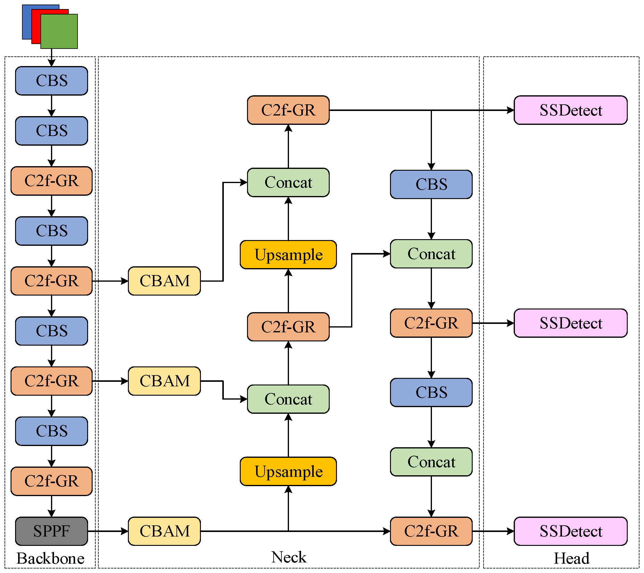
To achieve efficient grape leaf disease detection, this study implements three principal modifications to the YOLOv8 algorithm. First, the original C2f module is replaced with the C2f-GR module, which enhances gradient flow propagation and multi-scale detail capture while achieving lightweight architecture. Second, a CBAM is integrated to enable focused attention on critical lesion features. Finally, the detection head is optimized through cross-scale parameter sharing and independent batch normalization layers, resulting in the SSDetect (Shared Convolutional and Separated Batch Normalization Detection Head) head with enhanced parameter utilization and computational efficiency. The architecture of the GCS-YOLO structure is illustrated in Figure 3.

3.1. Lightweight Feature Extraction Module

To enable high-performance real-time detection of grape leaf diseases, this study proposes a lightweight feature extraction module named C2f-GR by enhancing the C2f structure through integration of the Ghost Module and RepConv.

3.1.1. Ghost Bottleneck

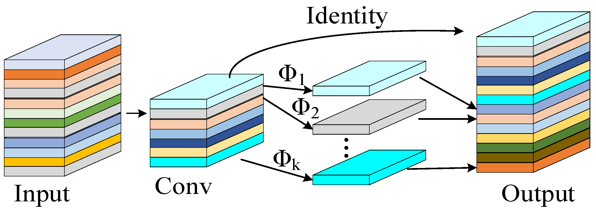
The incorporation of the Ghost Module reduces parameters and computational costs while maintaining accuracy. As illustrated in Figure 4, this module employs linear transformations to generate redundant intermediate feature maps. The fusion of differentially transformed feature maps significantly enhances the network’s feature representation capability. Figure 5 demonstrates that two Ghost Modules can be combined to form a Ghost Bottleneck. In the C2f-GR module, partial Bottleneck structures from the original C2f are replaced with these Ghost Bottlenecks [26].

For the Bottleneck, assuming the input feature map has height $h$ and width $w$, input channels $C_{\mathrm{in}}$, output channels $c_{\mathrm{out}}$, intermediate output channels $c_{out}/2$ between the two standard convolutions, and kernel size $k$, while omitting minor parameters and computations such as batch normalization (BN) and skip connections, the number of parameters and computational cost for Bottleneck are as follows:

$$P_{\mathrm{B}}={\displaystyle \frac{c_{\mathrm{out}}}{2}}\times k\times k\times C_{\mathrm{in}}+c_{\mathrm{out}}\times {\displaystyle \frac{c_{\mathrm{out}}}{2}}\times k\times k$$

(1)

$$F_{\mathrm{B}}=h\times w\times C_{\mathrm{in}}\times {\displaystyle \frac{c_{\mathrm{out}}}{2}}\times k\times k+{\displaystyle \frac{c_{\mathrm{out}}}{2}}\times h\times w\times c_{\mathrm{out}}\times k\times k$$

(2)

For the Ghost Bottleneck, maintaining identical input/output dimensions, let $c_{out}/2$ represent intermediate channels between Ghost Modules. Assuming each Ghost Module employs linear operations with a kernel size of $d$ and $s-1$ transformations per channel, the intermediate channels can be denoted as $c_{\mathrm{out}}/(2\times s)$ and $c_{\mathrm{out}}/s$, respectively. The number of parameters and computational cost for Ghost Bottleneck are as follows:

$$P_{\mathrm{G}}={\displaystyle \frac{c_{\mathrm{out}}}{2\times s}}\times k\times k\times C_{\mathrm{in}}+{\displaystyle \frac{c_{\mathrm{out}}}{2\times s}}\times d\times d\times 1+{\displaystyle \frac{c_{\mathrm{out}}}{s}}\times k\times k\times {\displaystyle \frac{c_{\mathrm{out}}}{2}}+{\displaystyle \frac{c_{\mathrm{out}}}{s}}\times d\times d\times 1$$

(3)

$$\begin{array}{l}{F}_{\mathrm{G}}=h\times w\times {\displaystyle \frac{c_{\mathrm{out}}}{2\times s}}\times C_{\mathrm{in}}\times k\times k+h\times w\times (s-1)\times {\displaystyle \frac{c_{\mathrm{out}}}{2\times s}}\times d\times d+h\times w\times {\displaystyle \frac{c_{\mathrm{out}}}{s}}\times k\\ \hspace{1em}\hspace{1em} \times k\times {\displaystyle \frac{c_{\mathrm{out}}}{2}}+h\times w\times (s-1)\times {\displaystyle \frac{c_{\mathrm{out}}}{s}}\times d\times d\end{array}$$

(4)

By comparing $F_{\mathrm{B}}$ and $F_{\mathrm{G}}$, the compression ratio can be calculated as follows:

$${\displaystyle \frac{F_{\mathrm{B}}}{F_{\mathrm{G}}}}={\displaystyle \frac{s\times (C_{\mathrm{in}}+c_{\mathrm{out}})\times k\times k}{3\times (s-1)\times d\times d+(c_{\mathrm{out}}+C_{\mathrm{in}})\times k\times k}}\approx {\displaystyle \frac{s\times (C_{\mathrm{in}}+c_{\mathrm{out}})}{C_{\mathrm{in}}+c_{\mathrm{out}}}}=s$$

(5)

where $d\times d$ has a similar magnitude as that of $k\times k$, and $3\times (s-1)\ll C_{\mathrm{in}}+c_{\mathrm{out}}$.

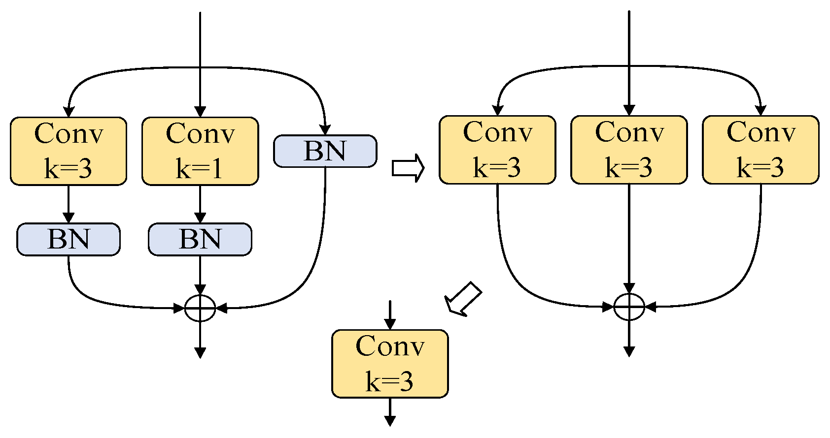
3.1.2. RepConv

While the Ghost Module significantly reduces parameters and computational costs, enabling multi-scale feature map fusion and enhanced feature extraction, it suffers from memory inefficiency. The multi-branch architecture necessitates retaining outputs from each branch until addition or concatenation operations, substantially increasing peak memory consumption. Moreover, excessive layer stacking prolongs model inference time. To address these limitations, we introduce Reparameterized Convolution (RepConv) into the gradient propagation branches of the C2f module, specifically replacing the first Bottleneck structure.

During training, RepConv integrates 3 × 3 convolution, 1 × 1 convolution, and batch normalization (BN) layers, alleviating gradient vanishing while strengthening gradient flow. During inference, structural reparameterization merges branch parameters into the primary 3 × 3 convolution, simultaneously improving detection accuracy and reducing inference latency. The fusion process between convolutional and BN layers is formulated as follows:

$$y={\displaystyle \frac{x-\mu }{\sqrt{{\sigma }^2+\epsilon }}}\times \gamma +\beta$$

(6)

where $\gamma$ and $\beta$ denote learnable parameters, $\mu$ is the mean, $\sigma$ is the variance, $\epsilon$ is a minimal non-zero constant, and $x$ is the convolutional output.

After substituting the convolution formula into the above equation, the transformation is provided as follows:

$$y={\displaystyle \frac{W\times x+b-\mu }{\sqrt{{\sigma }^2+\epsilon }}}\times \gamma +\beta ={\displaystyle \frac{\gamma \times W}{\sqrt{{\sigma }^2+\epsilon }}}\times x+{\displaystyle \frac{b-\mu }{\sqrt{{\sigma }^2+\epsilon }}}\times \gamma +\beta$$

(7)

where $W$ is the weight, and $b$ is the bias.

The aforementioned formula can be expressed in the following alternative form:

$$W_{\mathrm{f}}={\displaystyle \frac{\gamma \times W}{\sqrt{{\sigma }^2+\epsilon }}}$$

(8)

$$b_{\mathrm{f}}={\displaystyle \frac{b-\mu }{\sqrt{{\sigma }^2+\epsilon }}}\times \gamma +\beta$$

(9)

The fusion result can be expressed in a form similar to the convolution formula, and the formula is provided as follows:

$$y=W_{\mathrm{f}}\times x+b_{\mathrm{f}}$$

(10)

where $W_{\mathrm{f}}$ is the weight of the fused convolution, and $b_{\mathrm{f}}$ is the bias of the fused convolution.

The reparameterization process is shown in Figure 6. After fusing the convolutional and BN layers of each branch, the 1 × 1 convolutional kernels are expanded to 3 × 3 via zero-padding to handle branches with varying kernel sizes, while identity mappings are represented as 3 × 3 kernels with a central value of 1, and zeros are elsewhere. Finally, the convolution kernels and biases from all branches are summed to obtain the parameters for inference.

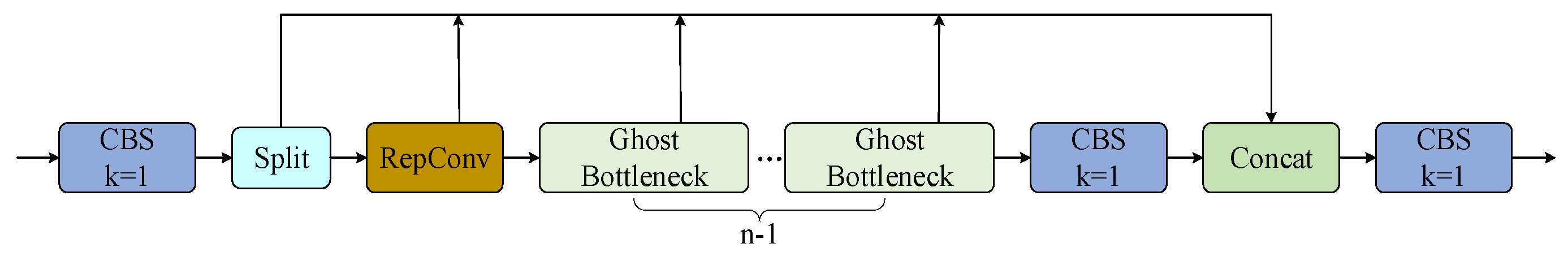
In the algorithm of this paper, the scaling factor in the C2f-GR module is 0.5, which means the output channels of RepConv are half of the output channels of the C2f-GR module, resulting in $c_{\mathrm{out}}/2$. Using $F_{\mathrm{B}}$, the computational cost of RepConv is calculated as $h\times w\times C_{\mathrm{in}}\times c_{\mathrm{out}}/2\times k\times k$, and dividing by $F_{\mathrm{B}}$ yields the ratio $1+C_{\mathrm{in}}/c_{\mathrm{out}}>1$ of the computational cost, thus achieving model lightweighting. The structure of the C2f-GR is shown in Figure 7.

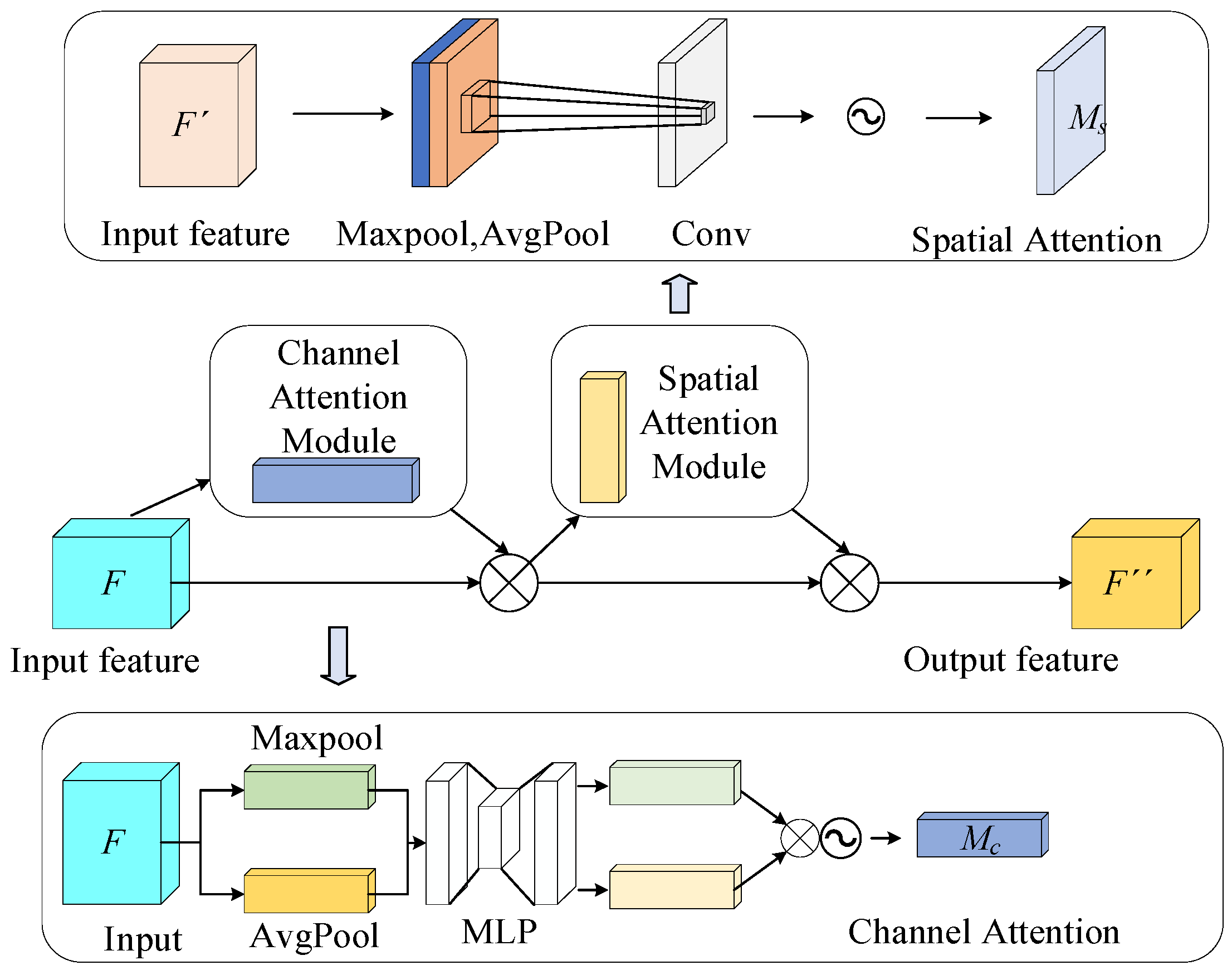
3.2. Introduction of CBAM

Convolution operations may accumulate redundant background information, leading to a decrease in the target attention and affecting detection accuracy. To enhance the model’s focus on key regions, we introduce the Convolutional Block Attention Module (CBAM) at the feature output layer of the backbone network. As shown in Figure 8, CBAM is an attention mechanism that combines spatial and channel attention to aggregate local information from feature maps. The channel attention module and the spatial attention module are two independent sub-modules of CBAM. This dual-module structure cleverly considers both channel and spatial dimensions, which aids the network in obtaining precise location and detailed information about the target region.

The channel attention module performs global max-pooling and global average-pooling on the input feature map and then feeds the pooled results into a Multi-Layer Perceptron (MLP). The outputs are summed and passed through a Sigmoid activation function to generate the channel attention weights. The MLP and weighted summation help the model adaptively determine the contribution of each pooling method.

The spatial attention module pools the input feature map to generate two feature maps, which are then concatenated into a single feature map via a 7 × 7 convolution and processed through a Sigmoid activation function to produce the final spatial attention weights.

The feature map is processed by the channel attention weights and spatial attention weights, removing irrelevant information through pixel-wise processing, which enables the model to focus more on the detection target information.

3.3. Introduction of SSDetect

In this paper, we improve the detection head of YOLOv8 by referencing the lightweight detection head from the high-accuracy model of RTMDet and designing the Shared Convolutional and Separated Batch Normalization Detection Head (SSDetect), which further reduces the number of parameters and computational cost of the model.

YOLO models typically use separate detection heads for different feature scales to enhance model capacity and achieve higher performance, but this significantly increases the parameter overhead. In fact, detectors with shared parameters suggest that the object features detected at different scales should be similar, though feature statistics still differ between layers. Therefore, batch normalization (BN) layers remain indispensable. Directly introducing BN layers into a shared parameter detection head would lead to errors in the moving average values. Hence, the detection head shares the convolutional layers, while the BN parameters are independently calculated to reduce the number of parameters in the head while maintaining accuracy.

As shown in Figure 9, the sizes and channel numbers of P3, P4, and P5 differ. To achieve shared convolutional layers, we first use a 1 × 1 convolution to adjust the channel number of P4 and P5 to match that of the smallest P3. Then, the feature maps are processed through two distinct 3 × 3 shared convolutional layers and two independent BN layers.

3.4. Evaluation Criteria

This experiment uses precision(P), recall(R), mean average precision (mAP50), and frames per second(FPS) to measure the performance of the model. Metrics, including GFLOPs, parameters (M), and model size (Mb), are employed to evaluate the scale of the model. The formulas are provided as follows:

$$P={\displaystyle \frac{\mathrm{TP}}{\mathrm{TP}+\mathrm{FP}}}$$

(11)

$$R={\displaystyle \frac{\mathrm{TP}}{\mathrm{TP}+\mathrm{FN}}}$$

(12)

$$\mathrm{AP}={\displaystyle {\int }_0^{1}P(R)\mathrm{d}R}$$

(13)

$$\mathrm{mAP}={\displaystyle \frac{1}{N}}{\displaystyle {\sum }_{i=1}^N{\mathrm{AP}}_{\mathrm{i}}}$$

(14)

where $\mathrm{TP}$ denotes the number of true positive samples, where the actual sample is positive and predicted as positive; $\mathrm{FP}$ represents the number of false positive samples, where the actual sample is negative but predicted as positive; $\mathrm{FN}$ indicates the number of false negative samples, where the actual sample is positive but predicted as negative; $\mathrm{AP}$ represents the average precision for a specific class; and $N$ denotes the number of classes.

4. Experiments and Analysis

4.1. Experimental Environment

In this study, the experimental environment consists of a high-performance computer configured with an Intel Core i5 processor, 16 GB of RAM, and an NVIDIA GeForce RTX 4060ti (8G) graphics card. Furthermore, to enhance the efficiency of deep learning experiments, this study adopts PyTorch 2.2.1 as the core framework and leverages CUDA acceleration for both model training and inference, ensuring computational efficiency and robust data processing throughout the experimental phase. The experimental model was trained for 200 epochs with a batch size of 32. The optimizer was configured to use Stochastic Gradient Descent (SGD) by default, accompanied by an initial learning rate of 0.01 and an Intersection over Union (IoU) threshold of 0.7.

4.2. Comparative Experiment of Different Lightweight Modules

To verify the effectiveness of adding RepConv, this paper replaces all Bottleneck modules in C2f with Ghost Bottleneck without adding RepConv and names the new module C2f-G. The experiments compare three lightweight modules—C3Ghost [28], ELAN-Tiny [32], and StarNet [33], with C2f-G and C2f-GR at the same positions in the YOLOv8 network, as shown in

Table 2. Comparative experiment results of different lightweight modules.

Lightweight Modules	mAP@0.5/%	Parameters/M	GFLOPs/G	FPS/s
None	94.9	3.01	8.2	153.8
ELAN-Tiny	94.0	2.31	6.0	161.7
StarNet	94.8	2.53	6.9	142.4
C3Ghost	94.4	1.99	5.6	122.8
C2f-G	94.5	1.98	5.6	124.8
C2f-GR	95.3	2.19	6.0	159.1

.

From the experimental results, it can be observed that ELAN-Tiny performs well in terms of computation and frame rate, but its mAP@0.5 decreases by 0.9%. StarNet achieves a higher mAP@0.5, but it has the highest number of parameters and computational cost. Both the C2f-G and C3Ghost modules, which incorporate the Ghost Module, achieve the greatest reduction in model complexity, but the excessive use of Ghost Modules leads to a deeper model, resulting in slower speed, with frame rates of 122.8 FPS and 124.8 FPS, respectively—significantly lower than the original model’s frame rate. C2f-GR has the highest mAP@0.5, with a reduction in model complexity, along with an improvement in frame rate. This indicates that introducing RepConv in C2f improves accuracy while reducing inference time. C2f-GR demonstrates the best overall performance, achieving a balance between accuracy, speed, and complexity.

4.3. Comparative Experimental Analysis of Attention Mechanisms

To investigate the detection performance of the CBAM on the dataset in this study, comparative experiments were conducted by integrating mainstream attention mechanisms SE [34], ECA [35], and EMA [36] at the same architectural location. The results are summarized in

Table 3. Results of comparisons between various attention mechanisms.

Attention	mAP@0.5/%	Parameters/M	GFLOPs/G	Model Size/MB
SE	95.7	3.02	8.3	6.4
ECA	95.2	3.01	8.2	6.2
EMA	96.6	3.09	8.4	6.4
CBAM	96.8	3.05	8.2	6.3

.

As illustrated in Table 3, with nearly the same number of parameters and computational cost, the model incorporating the CBAM achieves a mAP@0.5 of 96.8%, outperforming mainstream attention mechanisms such as SE, ECA, and EMA. Compared to the baseline YOLOv8 algorithm, this represents a 1.9% improvement in mAP@0.5. These results demonstrate that CBAM effectively focuses on critical feature information, enhances perception of grape leaf diseases, and enables more accurate localization and identification of infected regions.

4.4. Ablation Experiment

To verify the optimization effects of various improvement methods on the YOLOv8 algorithm, four sets of comparative experiments were designed, with training and testing conducted for each. The experiments followed the control variable method, and the results are presented in

Table 4. Ablation experiment results.

C2f-GR	CBAM	SSDetect	mAP@0.5/%	Parameters/M	GFLOPs/G	FPS/s
			94.9	3.01	8.2	153.8
√			95.3	2.19	6.0	159.1
	√		96.8	3.09	8.2	150.6
		√	94.7	2.36	6.5	141.3
√	√		96.5	2.27	6.0	148.7
√	√	√	96.2	1.63	4.5	136.9

.

The results show that after introducing the C2f-GR into the network, the number of parameters and computation were reduced by 27.2% and 26.8%, respectively, with a 0.4% increase in mAP@0.5 and a 5.3 FPS increase in frame rate, indicating that C2f-GR achieves lightweight optimization. After individually introducing the CBAM attention module, the mAP increased by 1.9%, while other metrics remained largely unchanged. When independently integrating the SSDetect shared-parameter detection head, the number of parameters and computational cost decreased by 21.6% and 20.7%, respectively, with only a 0.2% drop in mAP. After integrating the C2f-GR module into YOLOv8, the subsequent addition of the CBAM module further enhanced the model’s detection accuracy, achieving a 1.6% improvement in mAP while simultaneously reducing the number of parameters and computational cost by 24.6% and 20.7%, respectively. Overall, compared to the baseline model, the GCS-YOLO model achieved a 1.3% improvement in mAP while reducing the number of parameters and computational cost to 1.63 M (a 45.7% reduction) and 4.5 G (a 45.1% reduction) respectively, with an inference speed of 136.9 FPS.

4.5. Comparative Analysis of Algorithms

To verify the performance of the proposed improved model,

Table 5. Different algorithm comparison experiment.

Methods	mAP@0.5/%	Parameters/M	GFLOPs/G	Model Size/MB	FPS/s
Faster-RCNN	85.5	28.29	940.9	109.0	25.3
YOLOv8	94.9	3.01	8.2	6.2	153.8
YOLOv10	93.5	2.27	6.7	5.6	149.5
YOLOv5	94.4	2.51	7.2	5.2	134.2
YOLOv6-lite	90.3	1.06	0.8	2.5	80.2
YOLOv7-tiny	94.2	6.01	13.0	12.0	113.2
GCS-YOLO	96.2	1.63	4.5	3.6	136.9

presents a comparative experiment between the GCS-YOLO model and Faster-RCNN, YOLOv8, YOLOv10, YOLOv5, YOLOv6-lite, and YOLOv7-tiny.

The experimental results show that the Faster-RCNN model has high complexity and the worst detection accuracy, with an mAP of 85.5%, which is significantly lower than that of the YOLO series models. The YOLOv6-lite is the most lightweight model, but its mAP@0.5 is 90.3%, which is significantly lower than other mainstream models. In contrast, the proposed improved model has 1.63 M parameters, 4.5 G computation, and a model size of 3.5 MB, approximately half the size of other mainstream models. The mAP is 96.2%, an improvement of 1.3%, 2.7%, and 1.8% over YOLOv8, YOLOv10, and YOLOv5, respectively. Although the frame rate decreases compared to YOLOv10n and YOLOv8, it still meets the performance requirements for real-time detection. Overall, the GCS-YOLO model demonstrates significant performance advantages. Compared with other mainstream algorithms, the improved algorithm has minimal platform resource consumption while maintaining higher detection accuracy, making it suitable for production deployment and showing good application prospects.

4.6. Comparison of Results

To validate the performance differences between GCS-YOLO and the baseline model in detecting three types of grape leaf diseases, we compared the results of the two algorithms using Precision–Recall (P-R) curves. The P-R curve is a critical performance evaluation tool that visually illustrates the trade-off between precision and recall across varying detection confidence thresholds. The area under the P-R curve, known as Average Precision (AP), is a core metric in object detection. A higher AP value signifies a superior balance between precision and recall, reflecting stronger overall model performance. The P-R curves are shown in Figure 10. Notably, leaf blight exhibits the most significant improvement in the AP, with a 2.7% increase. The lesions of leaf blight are not only numerous but also small, making their detection more challenging compared to other categories. This substantial improvement primarily stems from the model’s enhanced ability to precisely focus on lesions of varying sizes and locations, thereby boosting detection performance. The improved model also demonstrates superior detection capabilities in other disease categories. Overall, the enhanced model achieves a 1.3% increase in mAP, outperforming the baseline model.

Figure 11 shows that in the detection results of YOLOv8, partial tiny lesions were missed in columns 1, 2, 5, and 6. Detecting these small lesions with sparse features is critical for the early identification of grape leaf diseases. In columns 3, 4, and 6, grape leaf diseases were misclassified as another disease with similar visual characteristics. After optimization, the improved model achieves precise detection of various grape leaf diseases. This improvement stems from the enhanced feature extraction capability and multi-scale feature representation of the model, which significantly improves its adaptability. Experimental results demonstrate that GCS-YOLO not only delivers superior detection performance but also achieves model lightweighting, making it highly suitable for real-time grape leaf disease detection.

5. Discussion

Overall, the algorithm proposed in this study demonstrates strong performance in balancing accuracy, speed, computational load, and memory usage. Compared to the YOLOv8 algorithm, the GCS-YOLO algorithm achieves reductions of 45.7% in parameters (1.63 M), 45.1% in computational cost (4.5 G), and 41.9% in model size (3.6 MB) while increasing the mAP by 1.3% (96.2%).

However, this study has certain limitations. To extract subtle features of lesions, the CBAM attention mechanism was introduced to enhance the model’s feature extraction capability for small targets. Although the improved model demonstrated significant improvements across multiple performance metrics, some undetectable micro-target information remains. In subsequent research, incorporating a small-target detection layer [37] could further enhance detection capabilities for minute targets. For scenarios constrained by device resources and processing speed, the C2f-GR and SSDetect lightweight architectures were implemented, effectively reducing the model’s parameter count and computational load. Nevertheless, such lightweight designs may adversely affect model adaptability, particularly when processing datasets captured in diverse environmental conditions. Future investigations could explore balancing computational complexity, parameter quantity, and detection accuracy through more lightweight techniques such as quantization [38], model pruning [39], and knowledge distillation [40,41], ensuring effective real-world agricultural applications of the model.

6. Conclusions

In real-time grape leaf disease detection, complex models often entail substantial computational costs and high resource demands, hindering widespread deployment. This paper proposes GCS-YOLO, a lightweight algorithm based on an improved YOLOv8 architecture. The algorithm replaces the original C2f module in YOLOv8 with a novel C2f-GR module that integrates Ghost Module and RepConv, effectively reducing the model’s parameter count and computational complexity. Additionally, the CBAM attention mechanism is incorporated to enhance the model’s focus on lesion regions, thereby improving detection accuracy. The detection head is further optimized using SSDetect, a lightweight head with cross-scale shared convolutions, to boost inference efficiency. The effectiveness of each module was validated through ablation studies, demonstrating the impact of individual improvements on model performance. The proposed model outperformed five other YOLO series variants, achieving a balanced performance with a mAP of 96.2%, 1.63 M parameters, 4.5 GFLOPs computational load, and a compact model size of 3.6 MB. In real-time performance testing, the model attained 136.9 FPS on an RTX 4060 Ti GPU, meeting the practical requirements for real-time processing in production environments. Although the GCS-YOLO algorithm proposed in this study achieved notable results in object detection, we recognize that its applicability and generalizability in real-world scenarios require further validation. Future work will focus on testing the model in more complex real-world environments, including varying lighting conditions and weather scenarios. Additionally, efforts will be made to further optimize the model’s computational efficiency to facilitate practical application and deployment on diverse edge devices.