A Comparative Study of Azure Custom Vision Versus Google Vision API Integrated into AI Custom Models Using Object Classification for Residential Waste

Abstract

The residential separate collection of waste is the first stage in waste recyclability for sustainable development. The paper focuses on designing and implementing a low-cost residential automatic waste sorting bin (RBin) for recycling, alleviating the user’s classification burden. Next, an analysis of two object identification and classification models was conducted to sort materials into the categories of cardboard, glass, plastic, and metal. A major challenge in sorting classification is distinguishing between glass and plastic due to their similar visual characteristics. The research assesses the performance of the Azure Custom Vision Service (ACVS) model, which achieves high accuracy on training data but underperforms in real-time applications, with an accuracy of 95.13%. In contrast, the second model, the Custom Waste Sorting Model (CWSM), demonstrates high accuracy (96.25%) during training and proves to be effective in real-time applications. The CWSM uses a two-tier approach, first identifying the object descriptively using the Google Vision API Service (GVAS) model, followed by classification through the CWSM, a predicate-based custom model. The CWSM employs the LbfgsMaximumEntropyMulti algorithm and a dataset of 1000 records for training, divided equally across the categories. This study proposes an innovative evaluation metric, the Weighted Classification Confidence Score (WCCS). The results show that the CWSM outperforms ACVS in real-world testing, achieving a real accuracy of 99.75% after applying the WCCS. The paper explores the importance of customized models over pre-implemented services when the model uses characteristics and not pixel-by-pixel examination.

1. Introduction

1.1. Problem Statement

The 21st century is marked by pressing topics such as smart cities, wastewater management, renewable energy, artificial intelligence (AI), climate change, and sustainable development. These issues are driving technological innovation and shaping the future of urbanization, environmental sustainability, and resource management [1].

To contribute to sustainable development by increasing recycling, all European Union (EU) countries had to transpose the EU regulations concerning the separate collection of waste (paper, metal, glass, paper, and plastic) by municipalities, including households, until July 2020 [2].

In the case of residential households, four different bins for each waste category must be installed, most likely next to each other, with different colors to be easily spotted by family members. Furthermore, the individual has to pay attention to choosing the right bin that corresponds to the waste category each time a specific waste is thrown. Sometimes, people could make involuntary mistakes by discarding the waste in the wrong bin, children up to a certain age find it difficult to choose the proper bin, children voluntarily dispose of waste in different bins just for fun, etc. Furthermore, the content of the four bins from inside the house must undergo an additional check when emptying into the corresponding four bigger bins from outside the house. This process is time consuming and is mandatory to prevent local authorities taxation for dumping waste in the wrong bin. Another issue is that several proposed bin setups from the specialized literature use algorithms that do not correctly identify the waste category.

The authors designed and implemented an AI-based separate waste collection bin for residential use with four bins for each waste category in a single unit to solve these issues. Moreover, the proposed prototype bin is used to validate two algorithms in correctly identifying the type of waste category. One proposed algorithm integrates a solution developed by Microsoft Azure Custom Vision Service 2024 (ACVS). This solution performs training on a large volume of data, with each volume corresponding to a specific class of waste. The second algorithm employs a Google Vision API Service 2024 (GVAS) solution, which generates a description of the identified object. This description provided by GVAS is further used to build a dataset. The new dataset ultimately serves to train a Custom Waste Sorting Model (CWSM) for the residential bin. The computed metrics highlight the advantage of the CWSM that can be integrated as real-time solutions that take the object and place it into the correct bin in a shorter time.

1.2. Paper Contributions

The main contributions of the paper are as follows:

• It investigates two approaches in the specialized literature regarding the automatic sorting of objects in the categories of cardboard, glass, paper, and metal;
• It designs and implements a low-cost residential automatic waste sorting bin (RBin) for recycling, which relieves the user of the task of determining the class in which the residual object should be placed;
• It examines pre-implemented services, such as ACVS and GVAS, to establish the correlation between the accuracy in the training dataset and the use in real-time application scenarios;
• It explores the number of images required for AI models to prevent overfitting and underfitting;
• It assesses customized models based on features in images, which can extrapolate characteristics for unseen objects and are thus not involved in the training phase;
• It builds the CWSM, which employs the LbfgsMaximumEntropyMulti algorithm, and the novelty lies in the transcription of the object’s description into words and training the model using the description as features;
• It develops a Weighted Classification Confidence Score (WCCS), an indicator that assesses the classification performance by analyzing the probability percentages for each waste category, normalized by their importance.

The paper is structured into six sections. Section 2 presents the reference works in the specialized literature, highlighting machine learning (ML) algorithms for the classification of household waste. Subsequently, Section 3 details the issues with the ACVS methodology and brings into question the inability of these models to be used in practice, considering the identification of the optimal number of images required for training, as well as their inability to extrapolate unknown characteristics of unseen objects in the analyzed category. It then analyzes the possibility of using GVAS to extract text descriptions of objects, which are then used to train a custom model that utilizes ML.NET. Furthermore, this section concludes with a unique performance evaluation indicator for the CWSM. The results are depicted in Section 4, highlighting the superiority of the CWSM, which uses text-level training. The discussion and limitations are presented in Section 5, whereas Section 6 focuses on the conclusions and future work.

2. Related Works

The specialized literature outlines two implementation directions regarding household waste classification. The first direction focuses on implementing AI solutions that, through various means, perform classification based on image acquisition, where the waste category of the identified object is detected. The second direction uses sensors and execution elements within an Internet of Things (IoT) infrastructure. The specialized literature also reports hybrid variants, including AI and IoT elements, managed through cloud computing technologies. Particular attention must be paid to the compatibility issue to form a functional hardware infrastructure [3].

2.1. ML Applied in Waste Classification

Friedrich et al. [4] investigate the maturity of data analytics in sensor-based and robot sorting in Austrian waste management. Expert interviews with stakeholders across the sensor sorting value chain highlighted varying levels of data maturity. The findings indicate that larger companies tend to have higher maturity levels in data analytics, with sensor and sorting machine manufacturers leading the way. ML is the primary technology in municipal solid waste management (MSWM), aiding in tasks from waste generation prediction to treatment and disposal [5]. ML algorithms, including artificial neural networks (ANNs), support vector machines (SVMs), and deep learning (DL) models, like convolutional neural networks (CNNs), optimize waste collection, classification, and recycling. ML tools are widely used in industry evolution [6,7]. Xia et al. [5] mention that waste sorting problems are treated in the literature using ML methods and forecasting. The authors note that challenges such as insufficient data, model interpretability, and integration need improvements in data sharing and real-time decision making for waste management. The classification problem is reduced to object identification based on image analyses [8], even when AI tools are involved in the process [9].

Giel and Kierzkowski [10] evaluate waste treatment systems using a fuzzy logic-based multi-criteria approach. It reviews existing methods, identifies gaps, and presents a model for municipal waste sorting. The model was applied to the Wrocław sorting facility. The prototype presented by Fu and Li [11] focuses on sorting trash using a robotic arm, ML, and computer vision (CV). The object is recognized using a camera image acquisition, followed by a classification process for identifying if the object is recyclable or non-recyclable. Fu and Li’s [11] research emphasizes the ML challenges related to object sizes and weights. Experiments revealed accuracy issues with glass and challenges handling larger items. The use of AI-based robotic sorting systems in municipal waste management, focusing on the ZRR2 robot installed at the Ecorparc4 sorting plant in Barcelona, is presented in the paper by Wilts et al. [12]. The robot, equipped with various sensors and DL algorithms, was trained to sort 13 types of waste. The results showed a sorting purity of up to 97%, with challenges such as the varying composition and morphology of municipal waste affecting recovery efficiency.

Lubongo and Alexandridis [13] examine the strengths and weaknesses of automated plastic waste sorting technologies by comparing manufacturers’ efficiency claims with the actual sorting results at Material Recovery Facilities (MRFs). The study identifies persistent challenges such as sorting tangled materials, black plastics, and mixed-material types. Fei et al. [14] present a smart trash bin concept. It integrates sensors, voice modules, and Arduino-controlled systems to measure capacity, humidity, and waste type.

Koliotasi et al. [15] examine waste management on the island of Corfu. The island has waste sorting issues because of tourist behavior. The authorities outline the need for automatic separation to improve waste management. Inefficient waste handling was seen as detrimental to Corfu’s image as a tourist destination, although stakeholders believe the issue is manageable with proper infrastructure and collaboration.

2.2. IoT Applied in Waste Classification

An IoT-driven waste management model using a hybrid predictive framework to track waste in a smart city employs a random forest algorithm to analyze waste data from interconnected smart bins, predicting when bins will fill and prioritizing waste collection. Each bin has sensors to monitor waste levels and detect hazardous gases. The model automates waste regulation, reducing manual intervention and sending alerts when bins are full or dangerous gases are detected [16]. The multimodal cascaded convolutional neural network (MCCNN) for efficient domestic waste classification, utilizing DSSD, YOLOv4, and Faster-RCNN, with a dataset of 30,000 images and 52 categories, is employed for the same purpose [17].

Feng et al. [18] introduce an intelligent waste sorting device with a lightweight GECM-EfficientNet model for waste classification. The model achieves 94.54% accuracy and a 146 ms inference time, deployed on an embedded system without internet dependence. The device automates waste sorting into four categories. The system is validated on two datasets, outperforming mainstream models in accuracy and real-time performance.

A Knowledge Extraction Model (KEM) for scheduling waste disposal from IoT-based smart waste bins using LoRa network media is introduced by Abidina et al. [19]. Key contributions include using various ML techniques to optimize waste management decisions. The Decision Tree (DT) method achieved the highest performance metrics, with an accuracy of 88.13%, a recall of 86.89%, and a precision of 93.61%. The study underlines the importance of using historical data for knowledge extraction and generating new rules for waste disposal scheduling.

Chazhoor et al. [20] benchmark six state-of-the-art DL models (AlexNet, ResNet-50, Res-NeXt, MobileNet_v2, DenseNet, and SqueezeNet) on the WaDaBa dataset for plastic waste classification using transfer learning. The dataset comprises five plastic types (PET, HDPE, PP, PS, and other) and contains 4000 images. ResNeXt achieved an 87.44% accuracy. MobileNet_v2, though slightly behind ResNeXt, demonstrated faster training times.

The ResNet-152 architecture for waste classification identifies different types of waste, such as plastic, paper, and metal. The process involves data collection, model training, evaluation, and fine tuning, followed by deployment for real-world waste classification. The model uses DL techniques, particularly transfer learning. The results indicate that ResNet-152 outperforms other models in waste classification tasks [21]. The TrashNet dataset is employed to classify six categories of waste, including cardboard, glass, plastic, paper, metal, and litter. The dataset includes 2527 high-resolution images. Several models are examined, combining DenseNet201 and MobileNet-v2 to create RWC-Net, a novel architecture with exceptional performance. RWC-Net outperformed existing models, achieving an F₁-Score of 95.01% and strong results across all waste categories, particularly excelling in distinguishing “cardboard” and “plastic”. The model was further validated using Class Activation Mapping (CAM) to visualize the focus areas of the model, confirming its ability to concentrate on relevant regions [22].

The article by Arbeláez-Estrada et al. [23] follows the Kitchenham guidelines for systematic literature reviews (SLRs) and focuses on the automatic segregation of waste using ML and physical enablers. Several studies have been analyzed, revealing a trend toward integrating AI technologies, such as image classification and sensor fusion, for waste identification. The importance of datasets, particularly the scarcity of data and the need for large, balanced datasets, is introduced in the paper as a direct path to high accuracy of the results. The paper also shows that material misclassification due to similarities between waste types, limited data, and real-world implementation issues, especially in uncontrolled environments, affects the model’s accuracy. The findings emphasize the potential of ML models, especially CNNs, in waste classification, with transfer learning techniques showing promise for enhancing model performance. Future research directions include addressing real-life complexities and improving the system through sensor integration and low-cost solutions. Additionally, image sensor analyses based on color identification technologies capture visual data. The process classifies waste types using the analyzed images [24].

The implementation of IoT technologies increases the capabilities of waste identification systems. IoT-enabled smart bins monitor waste levels in real time and provide data transmitted to a central system for analysis and action [25,26]. For example, a smart waste bin with ultrasonic sensors measures the fill level and sends alerts when it approaches capacity. Next, it optimizes collection routes and schedules [27,28]. In conjunction with the IoT, DL algorithms allow for advanced waste classification based on visual data [29,30].

In addition to traditional sensors, advanced technologies, such as Radio Frequency Identification (RFID) and X-ray imaging, are being explored for their potential in waste management. RFID tags are attached to waste items, while X-ray technology details the composition of waste materials [31,32]. Combining these technologies contributes to sustainability efforts by promoting recycling. Reducing landfill waste is another objective of combining AI technologies.

Integrating the IoT into waste management allows for real-time monitoring processes and making decisions based on data. For example, the IoT system presented by Belhiah et al. [33] has several hardware components, including GPS/GPRS modules for precise geolocation, IoT buttons for reporting green waste, and sensors for monitoring waste levels. Additionally, sweeping carts are equipped with devices that ensure data transmission and secure operation in challenging environments [34,35]. Implementing such smart waste systems has improved waste collection management, as shown by various case studies [36,37]. IoT platforms allow municipalities to analyze data for better operations management, leading to further improvements.

Smart bins with sensors automatically sort waste into various categories, reducing contamination in recyclable materials. Jain et al. [38] introduce a smart waste management system for urban areas, employing IoT technologies. The system uses sensors to monitor waste levels in bins and segregate waste into categories such as wet, dry, and metallic. The proposed prototypes have ultrasonic sensors to track waste levels. At the same time, these devices send real-time data to a cloud server. When bins are full or if a fire is detected, email alerts are sent to the authorities. This capability supports environmental goals in urban waste management [39]. The IoT in waste management also presents challenges, such as high upfront costs, strong infrastructure, and concerns about data privacy and security [40,41].

2.3. AI-IoT Applied in Waste Classification

Key achievements presented by [42,43] include the design of a prototype that monitors waste levels in real time, optimizes waste collection routes, and automates waste segregation. The modular system addresses various waste types, including plastics, glass, and waste electrical and electronic equipment (WEEE). Sosunova and Porras [40] examine existing research on smart waste management (SWM) systems within smart cities, particularly focusing on IoT-enabled technologies. Through a systematic review of 173 primary studies from over 3700 initially retrieved articles, the research identifies key elements in city-level and smart garbage bin (SGB)-related SWM systems. The analysis highlights the role of fill level, weight, temperature, air quality, motors, and servos in monitoring and managing waste. It also explores the stakeholders involved, including citizens, waste collection companies, and local authorities [44]. Automated systems using ML and CV technologies categorize waste into recyclable materials, boosting recycling rates and reducing the waste sent to landfills [45,46].

The proposed Waste Management 2.0 system leverages a low-cost ultrasonic sensor for fill-level monitoring, connects via a LoRaWAN and cellular network architecture, and ensures city-wide coverage. Extensive pilot studies across 10 locations in Lahore, Pakistan processed over 200 million data points, showing a 32% improvement in route efficiency, a 29% reduction in fuel consumption and emissions, and a 33% increase in waste processing throughput [47]. Dynamic route optimization for waste collection trucks, reducing fuel consumption and environmental impact, are discussed in the paper by Pardini et al. [48]. A multi-method review incorporating case studies, expert interviews, and document analysis presents in the paper by Kaluarachchi [49] the benefits of combining these infrastructures for urban waste management, stormwater control, and recreational spaces.

Abdullahi et al. [50] propose an automatic bin lid control activated by real-time waste level data, reducing unnecessary collection trips. A smart waste management system (SWMS) for Nusantara, Indonesia’s new state capital, employs ICT technologies and integrates sensors for real-time waste monitoring, categorization, and tracking [51]. It uses GPS-equipped waste vehicles and a central management platform to optimize waste collection. The proposed system triggers pickups when bins exceed capacity. This innovative framework supports Nusantara’s vision of being a smart city. In the same area, a smart waste bin placement system for rural Indonesia using the IoT, particularly the LoRa network, is presented in the paper by Abidin et al. [52]. The methodology incorporates a clustering technique to optimize bin placement by measuring the distance between households and the IoT server. The system uses geographical data to select bin locations based on proximity and clustering analysis. The approach was validated using the Davies–Bouldin Index (DBI) to assess cluster quality. This research proposes a novel way to manage waste in rural areas using the IoT.

Alhasan et al. [53] incorporate RetinaNet for object detection and Adagrad optimizer for classification. It was tested on a standard dataset, achieving a 99.62% accuracy. The system streamlines waste management processes. Longo et al. [54] present a 5G-enabled smart waste management system for university campuses. The use of 5G connectivity enables real-time data transmission. The system promotes eco-friendly practices and cost reduction in campus settings. The 5G Multi-access Edge Computing (MEC) integrates a CNN for automatic garbage sorting in the same field. MEC ensures low-latency, energy-efficient operations by processing data at the network edge. Longo et al. [55] include details on the system’s prototype and its design, implementation, and experimental validation.

Chauhan et al. [56] explore integrating circular economy principles with Industry 4.0 technologies to develop a smart healthcare waste disposal system for smart cities. Using the DEMATEL method, the study identifies seven key criteria, such as RFID labeling and GPS tracking for waste collection.

Anh Khoa et al. [57] introduce an innovative IoT-based waste management system designed for Ton Duc Thang University in Vietnam. The system uses ML and graph theory to predict the waste levels in trash bins. At the same time, the algorithm optimizes waste collection paths, affecting operational cost reduction. The study predicts the probability of trash bin fill levels using logistic regression.

3. Materials and Methods

This paper proposes a residential automatic waste sorting bin for recycling. It allows users to sort without being aware of the process. The main idea of this system is that the user throws the waste into the bin without thinking about which compartment the object should be placed in. The waste is automatically redirected to the corresponding compartment through the material sorting process.

This prototype has four separate compartments corresponding to the four major waste categories: glass, plastic, cardboard, and metal. This concept is based on implementing an automated waste sorting bin for recycling, using image processing algorithms and material recognition to determine the type of waste being thrown away. The system identifies materials from different types of waste, such as glass, plastic, cardboard, and metal, and directs these materials to a specific compartment without user intervention.

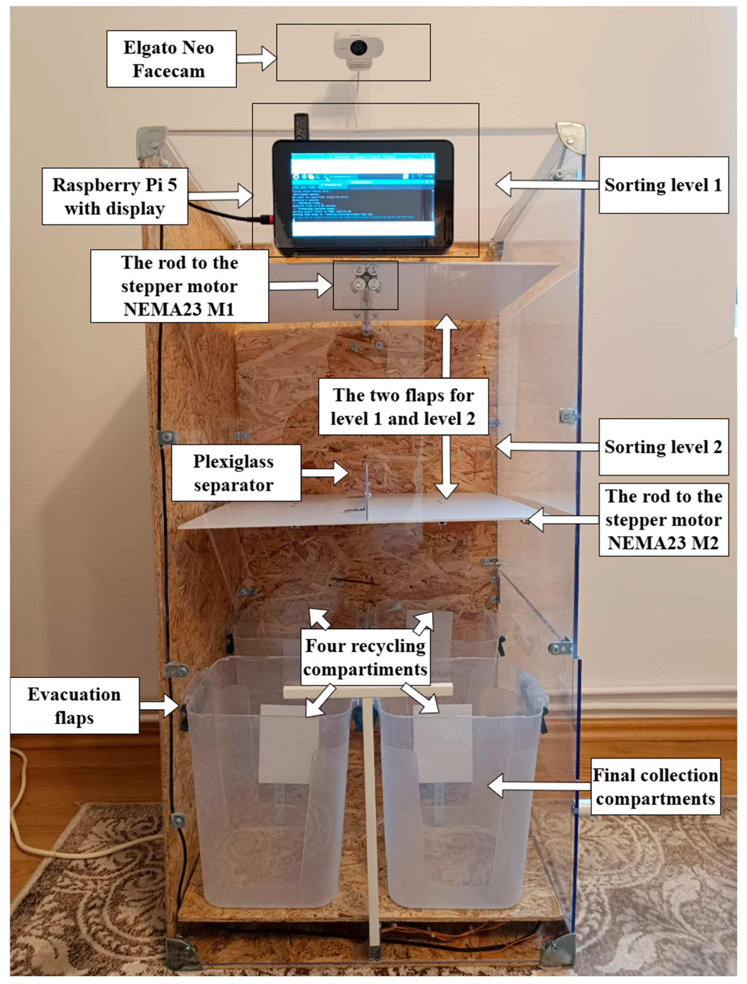
RBin is equipped with a two-level sorting mechanism ensuring redirection to the correct compartment, depending on the material types.

• Sorting level 1. At the top of the system, RBin has a flap that redirects an object to the left or right, depending on its characteristics. This flap is driven by a stepper motor, which ensures the object’s movement to the left or right, thus allowing an initial separation.
• Sorting level 2. After the object is redirected to one of the two initial paths (left or right), it reaches level 2 of sorting, where additional sorting occurs in the forward and backward directions. At this level, physical separator elements are placed along the object’s path, allowing the materials to be sorted into the corresponding containers.
• Final collection compartments. After the object has been sorted through the two levels, it reaches the final compartment corresponding to its material. Thus, the front-left compartment is designated for metal waste, the left-back compartment corresponds to plastic waste, the right-front compartment is designated for glass waste, and the right-back compartment collects cardboard.

There are separate elements of plexiglass on each level, so the objects cannot roll into the other plane once they reach level 2. RBin uses two NEMA23 stepper motors with TB6600 drivers, 4 A and 9–40 V, to control the redirection flaps of the objects.

RBin includes an integrated Elgato Neo Facecam to enable classification that captures images of the object placed on the collection flap. The employed algorithm for classification runs on a Raspberry Pi 5. The algorithm acquires the data as an image in real time, processes and extracts the information about the object, and makes the decisions for waste sorting. The visualization of the sorting process progress is reported to the RBin Raspberry Pi display, which shows information about the categories of collected materials. This screen was added as an additional informational tool for the user. However, in the commercial version of RBin, the visualization screen may be removed to reduce energy consumption and cost. Figure 1 presents the proposed hardware prototype previously described.

The total cost of the prototype is about 563 EUR. Raspberry Pi 5 is the central processing unit of the prototype, acquired for 89.9 EUR. It is paired with a Raspberry Pi display, priced at 69.8 EUR. The system is powered by a Pi5 27 W power supply with USB-C, which costs 13.4 EUR. Two NEMA 23 stepper motors control the sorting mechanisms’ movement. The total cost for these motors is 36 EUR. Along with the motors, motor drivers control them, which adds 16 EUR to the cost (

Table 1. Price of RBin components.

Component	Manufacturer	No. of Pieces	Price (EUR)
Raspberry Pi 5	Raspberry Pi Ltd., Pencoed, UK	1	89.9
Raspberry Pi display	Raspberry Pi Ltd., Pencoed, UK	1	69.8
Pi5 27 W power supply with USB-C	Raspberry Pi Ltd., Pencoed, UK	1	13.4
NEMA 23 stepper motors	MOONS’, Shanghai, China	2	36
Motor drivers	Toshiba, Tokyo, Japan	2	16
Elgato Neo Facecam	Corsair Gaming, Munich, Germany	1	92.1
Sandisk microSDXC Memory Card	Western Digital, Milpitas, CA, USA	1	35.6
Case for Raspberry Pi 5	Official Raspberry Pi Foundation, Cambridge, UK	1	12
Plexiglass separators	EuroPlastics, Wrocław, Poland	18	30.5
Plywood	Koskisen Group, Järvenpää, Finland	3	45.25
Flaps	Hettich, Kirchlengern, Germany	2	9.2
Recycling compartment	Waste Management Solutions Ltd., Birmingham, UK	4	15.5
Cable	Nexans, Paris, France	5	19.2
Joint components	Blum, Höchst, Austria	16	20.55
Other components	-	20	58
TOTAL	-	-	563

).

The physical structure of the prototype is built using plexiglass separators and materials for housing the components. These materials contribute to the overall cost of the prototype, which totals 563 EUR for the components used in the prototype. This breakdown reflects the key expenses associated with assembling the functional prototype for the RBin system, excluding any potential additional costs related to shipping or miscellaneous items. Moreover, the physical construction materials could be cheaper in other parts of the world, bringing the total cost of the prototype and the final product down.

The main challenge of the RBin is represented by the software infrastructure, which must perform the following actions in the shortest time possible:

• The camera captures the image;
• The image is sent to the classification service or algorithm;
• A response is received from the algorithm regarding the identified category;
• Motors are activated according to the identified category.

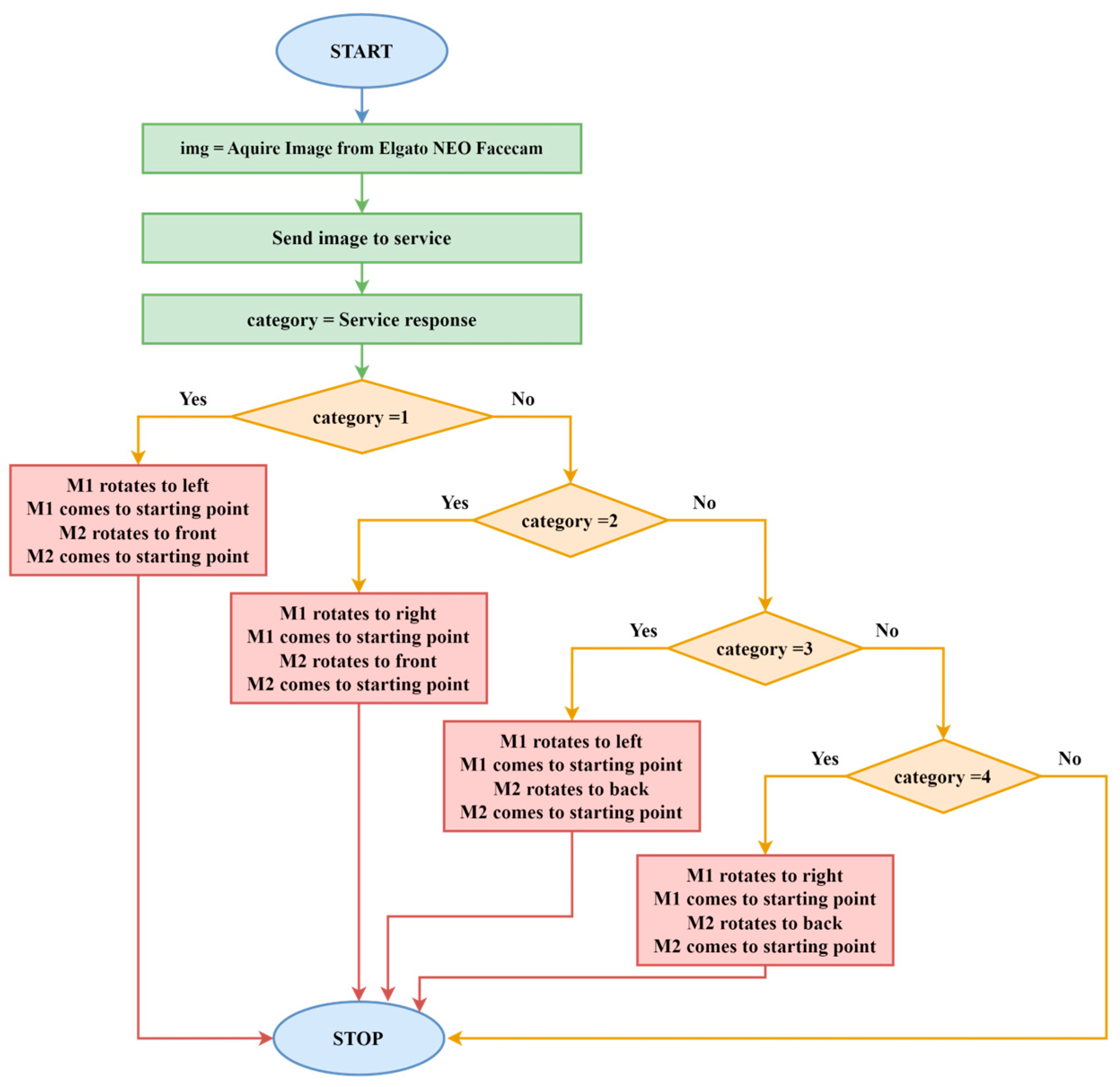
Figure 2 presents the block diagram of the category identification procedure. This flowchart describes the procedure for controlling the two NEMA23 stepper motors (M1 and M2) in response to a service’s classification result.

The procedure involves acquiring an image from the Elgato Neo Facecam, sending it for processing, and then controlling the motors based on the classification result.

• Start. The process begins by acquiring an image from the Elgato Neo Facecam;
• Send Image to Service. The captured image is sent to a service for classification;
• Service Response. The service processes the image and returns a classification result, referred to as glass, plastic, cardboard, and metal;
• Decision on Category. The returned category is evaluated. Based on the result, the motors will be controlled;
• Category 1. If the category equals 1, the stepper motor M1 rotates to the left, M1 returns to its starting point, and the stepper motor 2 (M2) rotates to the front and then returns to its starting point, as the object identified as metal was placed in the corresponding compartment;
• Category 2. If the category equals 2, M1 rotates to the right, M1 returns to the starting point, M2 rotates to the front, and M2 returns to its starting point. The second category is glass;
• Category 3. The plastic category is identified if the category equals 3. For plastic object identification, the M1 stepper motor rotates to the left, M1 returns to the starting point, M2 rotates to the back, and M2 returns to the starting point;
• Category 4. If the category equals 4, M1 rotates to the right, M1 returns to the starting point, M2 rotates to the back, and M2 returns to the starting point. The object identified as category 4 is cardboard.
• Stop. The process ends once the motors complete their rotations based on the classification.

The block diagram in Figure 2 outlines how motor movements (M1 and M2) are linked to the classification service’s response.

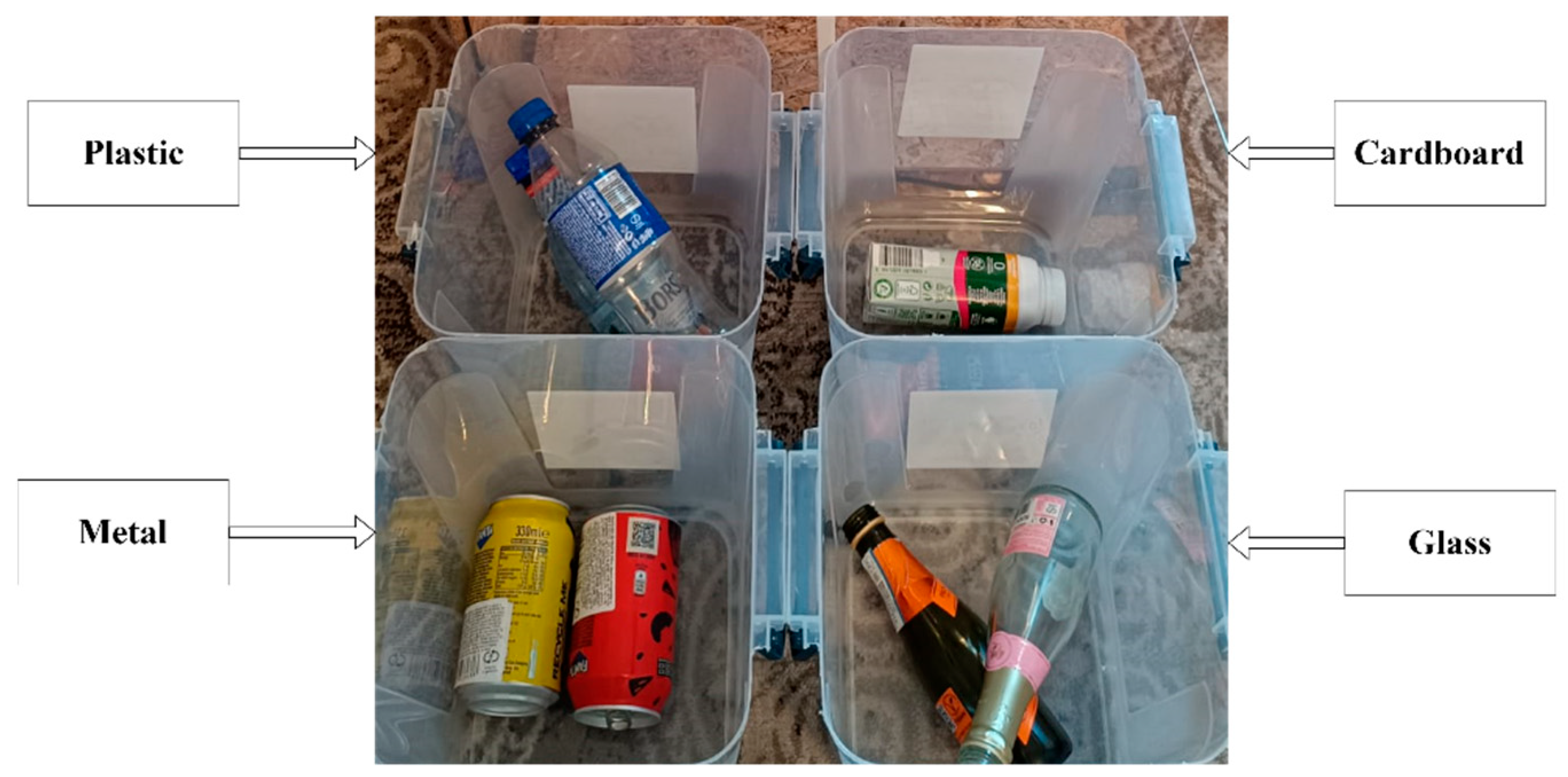
Figure 3 presents the four compartments corresponding to the glass, plastic, cardboard, and metal categories after extraction from the RBin using the evacuation flaps. Each compartment contains items that correspond to the specific material. For example, the plastic compartment holds plastic bottles, while the metal section includes cans and bottles made of metal. The compartments are detachable for easy emptying.

After analyzing these steps, it becomes clear that the central element is the classification algorithm. In this analysis, two types of algorithms were evaluated:

• The first is a cloud-based pre-implemented classification algorithm represented by ACVS. This first methodology for implementing the automatic sorting algorithm uses a pre-implemented classification service from Azure Custom Vision, which performs training in the cloud. In this context, the model is customized through the perspective of the images used in training rather than by modifying the rules written at the code level. In other words, the service’s recognition capability directly depends on the images used for training. The programmer implementing the service in the custom RBin algorithm does not know the characteristics analyzed by Custom Vision. Therefore, the programmer cannot adjust the recognition capabilities of the service in any way. This lack of flexibility affects the long-term classification abilities of RBin.
• The second is a custom algorithm that extracts key features of objects, associates them with the corresponding category, and builds the model based on these feature elements. The second methodology aims to extract key elements of the image using GVAS. These features are associated with the shapes identified at the object level and later correlated with a specific label. In this case, we will allocate values related to each label’s features identified at the object. We expect the number of associated values to be unique. This transcription of the object’s characteristics at the coordinate text level allows the classification issue to be approached uniquely. In other words, the problem is no longer one of image processing but rather a predicative one. By reducing the problem to the analysis of predicate sequences, we aim to create a pattern based on these values. This pattern can then be transposed through the identification of a specific category. Based on this aspect of uniqueness, we aim to address the classification problem applied in household waste sorting. The final model responsible for the classification problem is the CWSM.

The two algorithms are assessed using standard classification evaluation metrics: accuracy, precision, recall, and F₁-Score. Additionally, they are analyzed in terms of response time.

The quality of classification algorithms directly depends on the dataset volume used. It should be noted that within a category, there are many products; for each product, multiple pictures are needed to represent the product in different poses. In other words, the product must be captured in various positions, with varying degrees of degradation, in all possible versions. For example, if a brand associated with a bottle of wine contains different labels for different varieties, then each array is a different product. Also, classification algorithms are influenced by the content present in the background images. In the case of this work, this issue does not apply because in the upper part of the bin, the element on which the object is placed is always the same, remaining unchanged.

In a brief analysis, the two algorithms employed in this paper have four classification categories. Assuming that each category hypothetically has two associated products, training requires a minimum of 20 images per product. This means that for the given scenario, 160 images are needed. Exploiting the logic of this example, it is concluded that classification algorithms based on image training are a utopia that is impossible to use in practice due to the large volume of data. This aspect will be demonstrated as follows.

The authors emphasize the importance of classification algorithms based on images used for academic training. However, in practice, classification algorithms should include features of these objects so that they have a degree of generalization, allowing them to adapt to products they have never seen. In the authors’ opinion, building a dataset that includes all existing products is impossible.

3.1. Azure Custom Vision Methodology

The methodology used for category identification employs ACVS. The training process begins with collecting labeled images representing different categories. The model classifies waste, so plastic, metal, paper, and glass images are collected and labeled accordingly. The labeled images represent the entire training dataset. The dataset is uploaded to ACVS for training. The biggest problem of the dataset is finding the optimum number of images for each category. The construction of the dataset must adhere to the following rules:

• The AI engineer must determine the number of images for each category so that the model does not overfit, meaning it does not adapt too much to the specific features of the class. Also, the engineer must ensure that the model is not undertrained, meaning there are not enough images for each category to identify the features that distinguish categories from one another;
• The data engineer must ensure the variability of each category through the data. This means that some categories require more training images if there is a wide variety of unique tuples within the class, such as plastic, which comes in many types and where objects may have different shapes;
• All environmental conditions must be represented by acquiring images from different angles, light types (natural and artificial), varying brightness levels, and shadows from various angles.

To prevent the model from being biased toward a particular class, we impose a similar number of images for the training dataset across categories in ACVS. If one class has more images than another, the model may learn to favor that class. For this reason, we impose an equal number of images for each category. To demonstrate this statement, for ACVS, we initially built a dataset with 100 images per category. Even though a smaller number of images may be sufficient for very simple categories (like metal), we imposed the value of 100 to prevent bias. Later, in the second stage of training, ACVS is modified with a smaller number of images for the metal class and a larger number for the plastic class. In the third scenario, we employed 1000 images, 250 for each category.

ACVS uses ML algorithms to train the model. The model learns to identify image patterns corresponding to the labeled categories. The training process involves using these images to teach the model to predict the category for new, unseen images.

The process begins by capturing an image, which is then sent to ACVS. The service processes the image and classifies it into predefined categories based on the model trained using labeled data. The classification result is returned, indicating which category the image belongs to. If the model does not predict with the expected accuracy, it can be re-trained in a new iteration by adjusting the number of images for the discriminated category.

After establishing 1000 images for each category, we validated the model’s performance on a validation dataset. For testing, we used two types of validation data: one similar to the objects used in the training process and the second type consisting of completely different data from the training set but belonging to the same category. The significance of the second type of validation corresponds to the model’s ability to distinguish between categories by discriminating features.

The authors introduce the concept of discrimination when the model memorizes the specific objects it saw during training. The model needs to generalize distinctive features of the object. Based on these unique features, it must correctly identify new, unseen objects from the same category. By focusing on this validation, we evaluate the model’s true capacity to differentiate between categories (such as identifying a plastic bottle versus a glass one) by recognizing and discriminating the key features defining each category.

Suppose the model shows signs of overfitting (for example, excellent performance on the training set but poor performance on the validation set). In that case, the model has too many images and is overfitted. If the model is underfitted (for example, poor performance on the training and validation sets), more images are added.

The standard metrics used to assess the model performance are accuracy, precision, recall, AP (average precision), and F₁-Score [6,58].

• Accuracy is the weight of true predictions out of all predictions and is computed with Equation (1).

$$\mathrm{A}\mathrm{c}\mathrm{c}\mathrm{u}\mathrm{r}\mathrm{a}\mathrm{c}\mathrm{y}={\displaystyle \frac{\mathrm{T}\mathrm{P}+\mathrm{T}\mathrm{N}}{\mathrm{T}\mathrm{P}+\mathrm{T}\mathrm{N}+\mathrm{F}\mathrm{P}+\mathrm{F}\mathrm{N}}}\times 100[\%]$$

(1)

• Precision is determined by Equation (2) as a true positive (TP) prediction of all positive predictions.

$$\mathrm{P}\mathrm{r}\mathrm{e}\mathrm{c}\mathrm{i}\mathrm{s}\mathrm{i}\mathrm{o}\mathrm{n}={\displaystyle \frac{\mathrm{T}\mathrm{P}}{\mathrm{T}\mathrm{P}+\mathrm{F}\mathrm{P}}}\times 100[\%]$$

(2)

• Recall represents the effective identification of true predictions. It is calculated by Equation (3).

$$\mathrm{R}\mathrm{e}\mathrm{c}\mathrm{a}\mathrm{l}\mathrm{l}={\displaystyle \frac{\mathrm{T}\mathrm{P}}{\mathrm{T}\mathrm{P}+\mathrm{F}\mathrm{N}}}\times 100[\%]$$

(3)

• AP is calculated by Equation (4) and consists of the area beneath the precision–recall curve.

$$\mathrm{A}\mathrm{P}={\int }_0^1\mathrm{P}\mathrm{r}\mathrm{e}\mathrm{c}\mathrm{i}\mathrm{s}\mathrm{i}\mathrm{o}\mathrm{n}\left(\mathrm{R}\mathrm{e}\mathrm{c}\mathrm{a}\mathrm{l}\mathrm{l}\right)\mathrm{d}\mathrm{R}\mathrm{e}\mathrm{c}\mathrm{a}\mathrm{l}\mathrm{l} [\mathrm{\%}]$$

(4)

• F₁-Score is determined based on precision and recall with Equation (5):

$${\mathrm{F}}_1-\mathrm{S}\mathrm{c}\mathrm{o}\mathrm{r}\mathrm{e}=2\times {\displaystyle \frac{\mathrm{P}\mathrm{r}\mathrm{e}\mathrm{c}\mathrm{i}\mathrm{s}\mathrm{i}\mathrm{o}\mathrm{n}\times \mathrm{R}\mathrm{e}\mathrm{c}\mathrm{a}\mathrm{l}\mathrm{l}}{\mathrm{P}\mathrm{r}\mathrm{e}\mathrm{c}\mathrm{i}\mathrm{s}\mathrm{i}\mathrm{o}\mathrm{n}+\mathrm{R}\mathrm{e}\mathrm{c}\mathrm{a}\mathrm{l}\mathrm{l}}}\times 100 [\mathrm{\%}]$$

(5)

At this stage, we computed four of the above-mentioned metrics, namely, accuracy, precision, recall, and AP, to assess whether the model performed well enough to classify waste correctly.

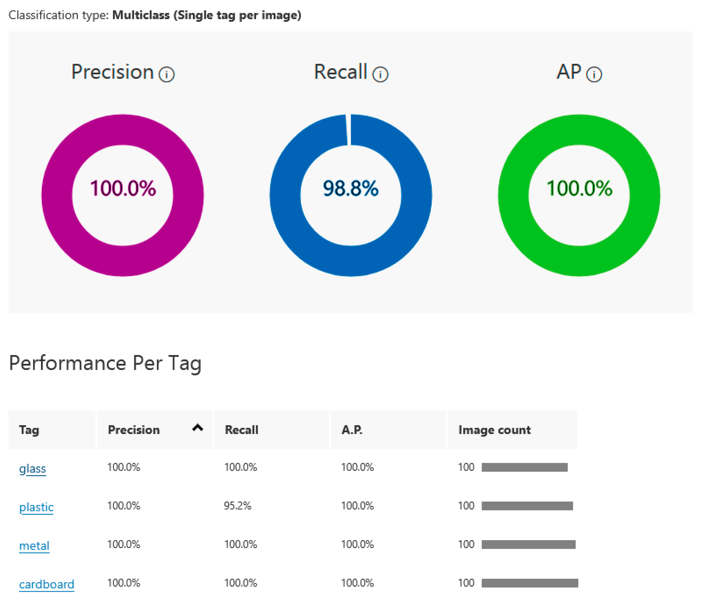
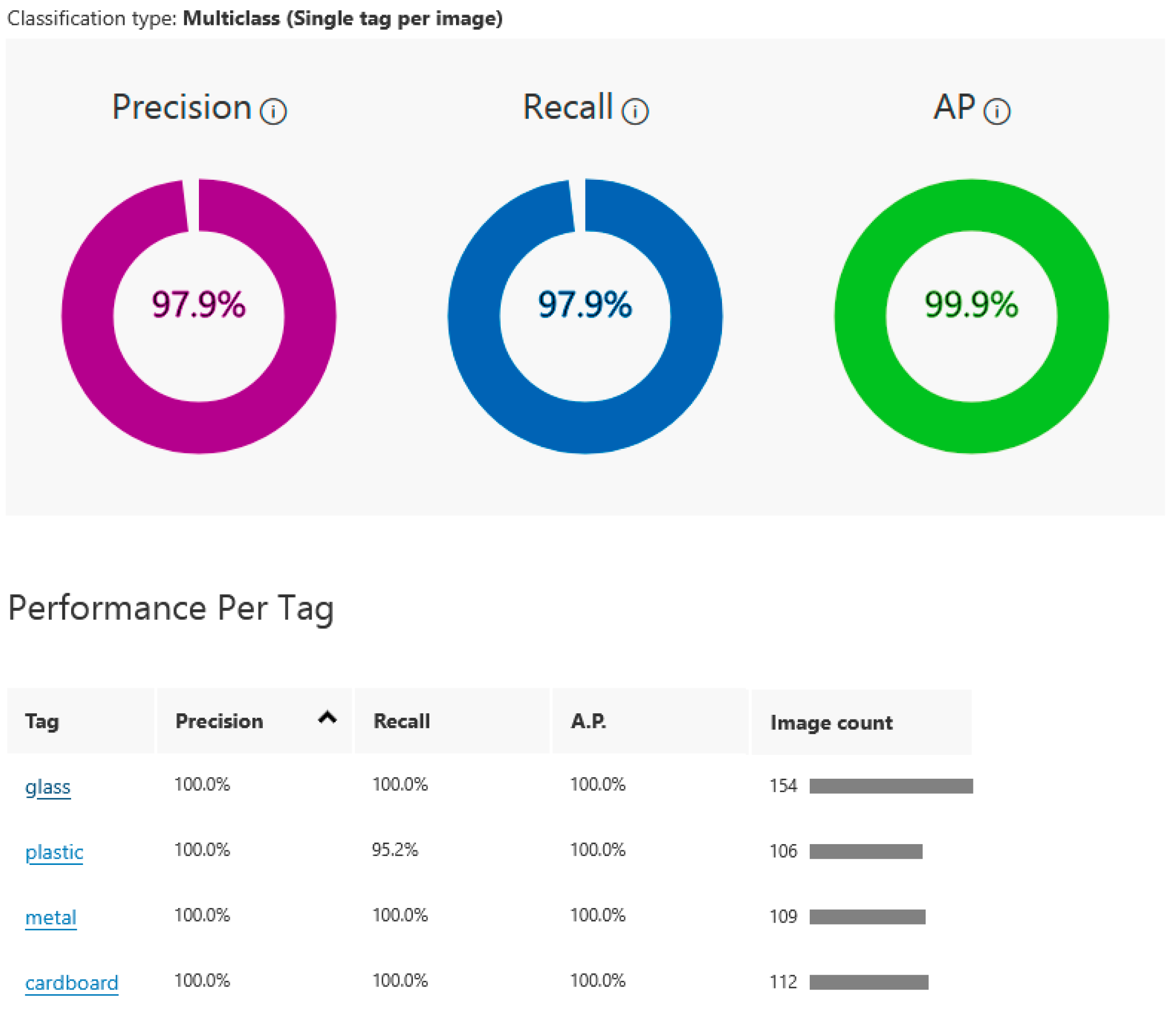
The ACVS performance parameters of the model are presented in Figure 4. The obtained values indicate that the model for classifying waste categories (glass, plastic, metal, and cardboard) has performed exceptionally well in a multi-class classification task with 100 images per category. The model achieved a perfect 100% precision. At the same time, the model identifies 98.8% of all true instances of the categories in the validation dataset. This is a strong result, though it suggests that there may be a very small number of missed predictions. The 100% AP score suggests that across all categories, the model’s predictions were well calibrated. The model has 100% precision, meaning every glass image was classified correctly. The recall is also 100%, indicating that all glass instances were detected.

In Figure 4, the glass category’s AP is also perfect. The precision for plastic is again 100%, but the recall drops slightly to 95.2%, meaning the model missed a small number of plastic items. However, the AP is still 100%, reflecting well-calibrated predictions for this category. Similar to glass and plastic, metal is classified with 100% precision and a very high recall of 100%, indicating perfect performance. The cardboard category also performs flawlessly with 100% precision, 100% recall, and 100% AP. Each category was tested with 100 images, ensuring the model was evaluated across a balanced number of examples for all categories. The model has performed excellently across all categories with near-perfect scores in precision, recall, and average precision. Considering the overall high performance, the slight dip in recall for the plastic category (95.2%) should not raise concerns.

In a second iteration of the training process, we try to increase the recall by adjusting the number of images. The results of the performance parameters obtained are presented in Figure 5. The minor decrease in performance (precision and recall dropping from 100% to 97.9%) indicates that as the dataset expands, the model starts to make more general predictions based on a broader set of features. The slightly lower recall for plastic indicates that the model has to deal with more varied plastic types, reducing its sensitivity to certain plastic objects.

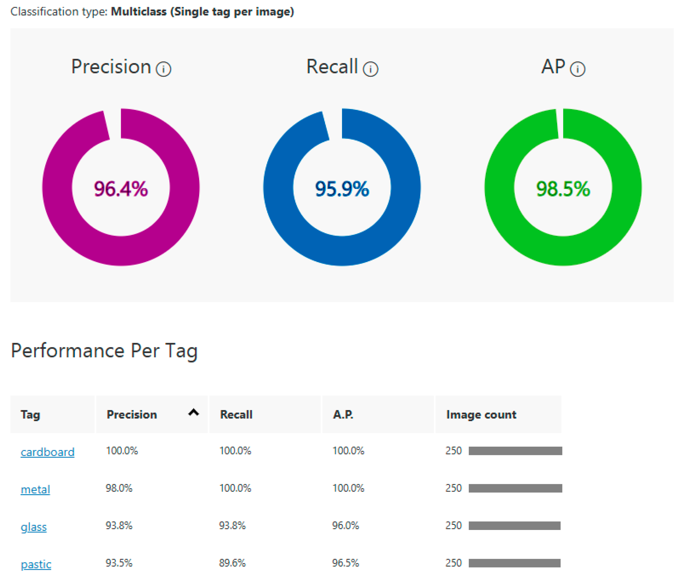
In the third iteration, the model was re-trained using 250 images for each category. In this third iteration, despite the number of images being the same, the obtained precision was 96.4%, the recall was 95.9%, and the AP was 98.5%. For the cardboard category, the values for all metrics were 100%, while for the metal category, the precision was 98%. The glass category achieved, after training, a precision of 93.8%, a recall of 93.8%, and an AP of 96.0%. Regarding the plastic category, it obtained a precision of 93.5%, a recall of 89.6%, and an AP of 96.5%. The results of this iteration are summarized in Figure 6.

While the model performed excellently in both tests, the number of images per category has slightly decreased the recall and precision for certain categories, like plastic. The minor decrease in performance results from balancing between training with more data and preventing overfitting. For the tests section, we will use the third iteration as an equitable measure for model comparison.

3.2. CWSM Based on Google Cloud Methodology

GVAS is used by the RBin algorithm to label objects at the image level. To achieve this identification, we used the LABEL_DETECTION feature of GVAS. This feature allowed for the identification of the object under analysis in the image. Subsequently, the object was described by label–confidence score correspondence. Since the service returns multiple labels for a single object, the predicate string is built as a JSON that includes all the local labels the service provides. The analysis does not contain elements with a confidence score below 50%. Building the training dataset for the custom model is performed using the JSON format, as shown in the example below.

{

“metal”: { “Drink can”, “Steel and tin cans”, “Aluminum can”, “Tin” },

“metal”: { “Transparency”, “Hardwood”, “Plastic”, “Plywood” },

…

“cardboard”: { “Transparency”, “Box”, “Shipping Box”, “Packaging and labeling” },

“cardboard”: { “Transparency”, “Plywood” },

…

“plastic”: { “Liquid”, “Glass”, “Bottle”, “Transparency”, “Plastic”, “Plastic bottle”, “Bottled water” },

“plastic”: { “Liquid” },

…

“glass”: { “Bottle”, “Alcoholic drink”, “Glass bottle”, “Glass”, “Liquor”, “Transparency”, “Champagne” },

“glass”: { “Alcoholic drink”, “Bottle”, “Glass bottle”, “Liquor”, “Beer bottle”, “Wine bottle”, “Varnish”, “Wine”, “Beer” },

…

}

The dataset is constructed using the same images employed for ACVS. After building the file containing the label-JSON correspondences using GVAS, we built the model using the ML.NET Data Classification component. The GVAS training dataset contains 1000 feature–label pairs. After training the final model, we identify the CWSM.

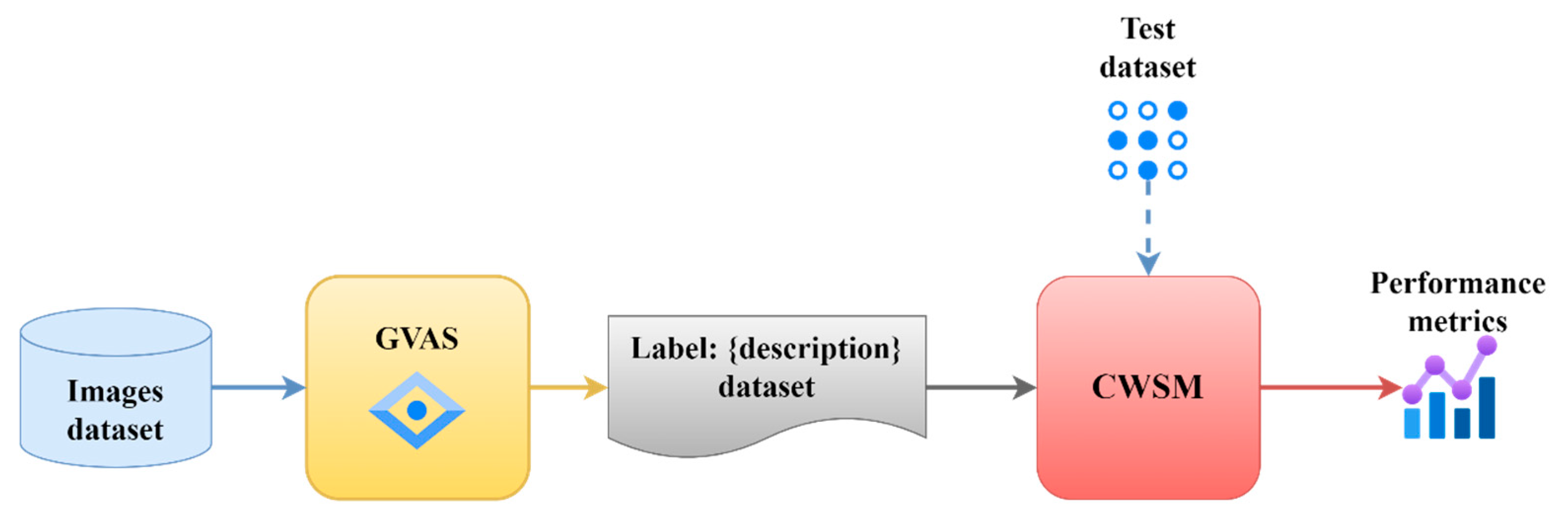
The process presented in Figure 7 starts with the image dataset involved in the training process. These images are inputs for the model GVAS (the service used to generate labels and descriptions). GVAS assigns local labels to each object, creating a dataset with descriptions for each image. Once the labeled dataset is ready, it is passed to the CWSM, where the model is trained. During training, the model uses the labeled dataset to learn the features and patterns of the different categories in the images.

Five ML algorithms were analyzed for the CWSM, but LbfgsMaximumEntropyMulti achieved the highest performance. However, this result highlights a performance gap compared to the accuracy achieved by the ACVS model, which demonstrated a 95.13% accuracy.

3.3. Weighted Classification Confidence Score

For the comparative evaluation of the models, we move beyond the standard performance metrics, such as accuracy, precision, and recall, which were previously analyzed. Additionally, we will introduce a new indicator incorporating an object’s percentage probabilities in each category. In this way, we analyze the capacity of the model to extrapolate knowledge.

The indicator, the Weighted Classification Confidence Score (WCCS), assesses the classification performance by analyzing the probability percentages for each waste category, normalized by their importance, and addresses cases where multiple probabilities for the same category are present. The WCCS is computed by Equation (6).

$$WCCS={\displaystyle \frac{{\sum }_{k=1}^4{P}_k\times (1-{\delta }_k)}{1+Variance(P_1,P_2,\dots ,P_N)}}\times 100[\%],$$

(6)

where

WCCS is the Weighted Classification Confidence Score;

P_k is the associated probability for each waste category;

δ_k is the overlapping probabilities within the same waste category (set to zero if no multiple predictions for the same category are provided);

N is the number of identified probabilities;

Variance(P₁, P₂, …, P_N) measures how spread out the probabilities are. A higher variance means the model is more confident in one waste category (dominant), and a lower variance means indecision between waste categories. It is computed by Equation (7).

$$Variance\left(P_1,P_2,\dots ,P_N\right)={\displaystyle \frac{{\sum }_{k=1}^N{(P_k-\mu )}^2}{N}},$$

(7)

where

μ is the mean of the probabilities, calculated by Equation (8).

$$\mu ={\displaystyle \frac{{\sum }_{k=1}^N{P}_k}{N}},$$

(8)

Including percentage probabilities is valuable because it provides additional context beyond binary or single-label predictions. For instance, considering that an object belongs to the plastic category, the model indicates a 90% probability for plastic, 7% for glass, and 3% for cardboard. This information helps calculate the WCCS with the main purpose of identifying the trust in the predicted category. The proposed WCCS has the following advantages:

• It captures the model’s confidence for all categories simultaneously, ensuring that borderline cases are represented;
• It penalizes over-confidence or misclassification when multiple probabilities overlap for the same category;
• It incorporates waste category-specific importance through weights;
• It measures the performance of waste category-specific complexities.

If the denominator category has a lower level, the WCCS value increases. When the dominant category is identified, the WCCS’s confidence in its prediction decreases.

Next, we analyze two opposite scenarios. The first is the perfect classification; the first class has 100% identification, and the other three have 0%. For this case, the mean probability μ is 0.25. The variance is calculated as follows:

$$Variance={\displaystyle \frac{{(1-0.25)}^2+{(0-0.25)}^2+{(0-0.25)}^2+{(0-0.25)}^2}{4}}=0.1875$$

Using this variance value, the WCSS is as follows:

$$WCCS={\displaystyle \frac{1+0+0+0}{1+0.1875}}\times 100=0.842\times 100=84.2\%$$

As a result, the perfect classification scenario is to identify the WCCS with the 84.2% value. The scenario where all classes are identified with the same 25% value is analyzed at the opposite corner. The mean value is calculated as 0.25. The variance is as follows:

$$Variance={\displaystyle \frac{{(0.25-0.25)}^2+{(0.25-0.25)}^2+{(0.25-0.25)}^2+{(0.25-0.25)}^2}{4}}=0$$

Next, the WCCS is calculated as follows:

$$WCCS={\displaystyle \frac{0.25+0.25+0.25+0.25}{1+0}}\times 100=1.00\times 100=100\%$$

Using this reasoning, we conclude that the WCSS has an 84.2% value for the ideal scenario. When the CWSM value increases, the meaning of this behavior is the incapacity of the model to distinguish between categories. The ACVS model’s and the CWSM’s performance is evaluated using objects that have never been encountered during the training process. These objects belong to a typology not employed during the model training phase. We analyze this data topology to identify the model’s behavior when unseen data are provided. We expect the best model to approach the identification of the real category.

This testing methodology assesses whether the models distinguish between the four waste categories. The proposed WCCS calculates the trust level of the predicted category for unseen objects and typologies.

4. Results

The models are implemented for evaluation using the C# programming language. The same training and testing images were used to ensure fairness in the comparative analysis of the two proposed models, ACVS and the CWSM. This way, the obtained results can be compared without discriminating against one of the methods. The training dataset includes 1000 images, and the testing dataset has 400 images, uniformly distributed among the four analyzed categories. This size allows for evaluating the models’ ability to classify objects correctly. Increasing the number of training images is not a solution regarding the generalization of a model. The model’s performance should come precisely from its ability to extract a category’s basic features and generalize for all objects in that class. From this context, the problem of waste classification also arises. It is very difficult to build a dataset containing all existing objects in reality, and these objects must be subjected to all possible contexts of angle, lighting, and quality contexts. Building such a dataset is a utopic ideal.

The dataset was constructed for training and validating the models by balancing the distribution across the four waste categories: plastic, glass, cardboard, and metal. The images used to build the dataset were collected from multiple sources to ensure the variability needed for the model to generalize to new objects. These sources include the following:

• Public databases with images of recyclable objects [59];
• Images captured using a mobile phone, including damaged or deformed objects, to mimic real-life scenarios;
• Images captured using the camera of the proposed prototype.

The dataset includes images from different angles and under various lighting conditions (natural, artificial, low lighting, partial shading). This strategy allows for assessing the generalization capability of the two models in a comparative analysis. In this way, the models are not trained exclusively on a limited type of image and can make predictions about unknown objects.

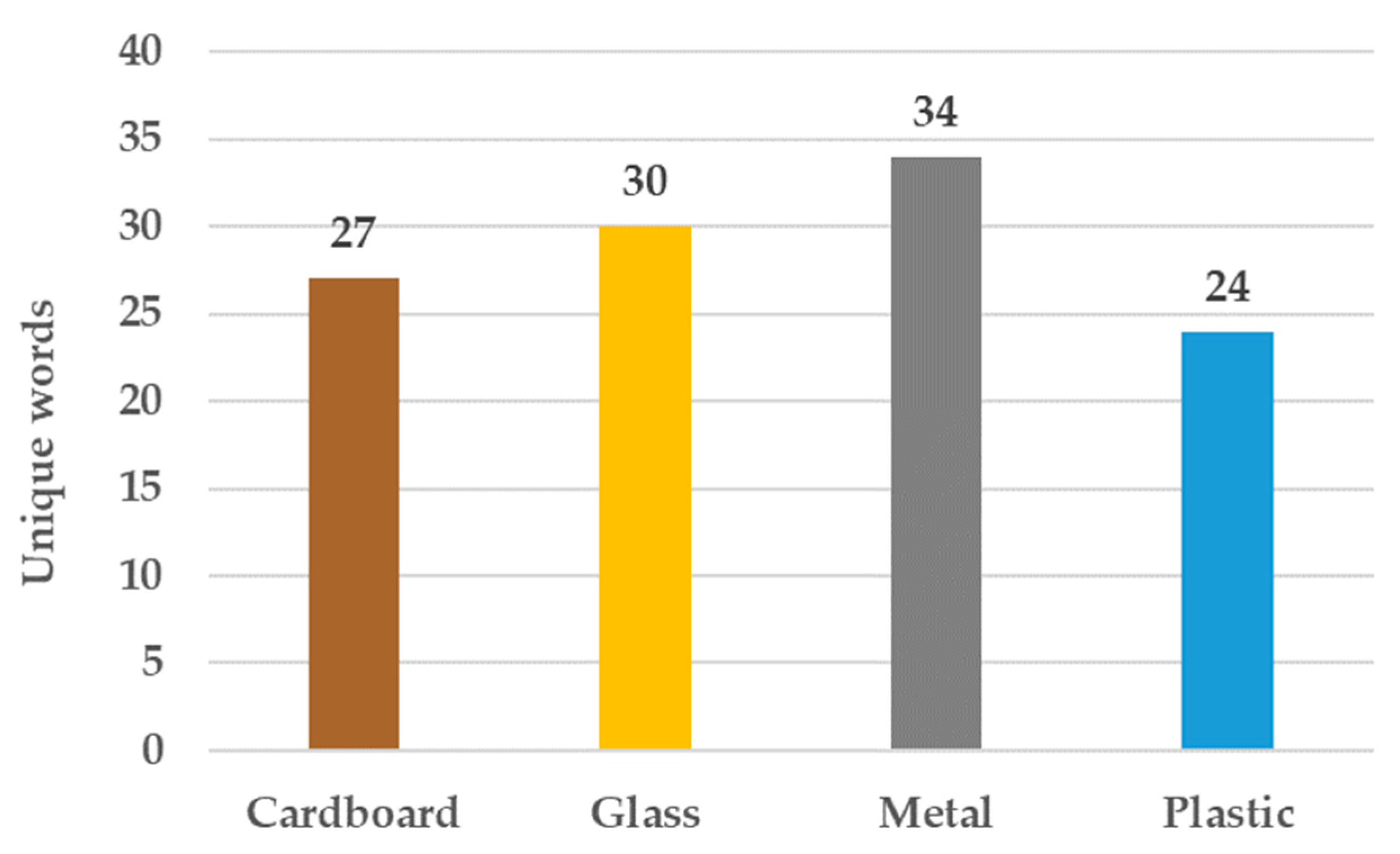
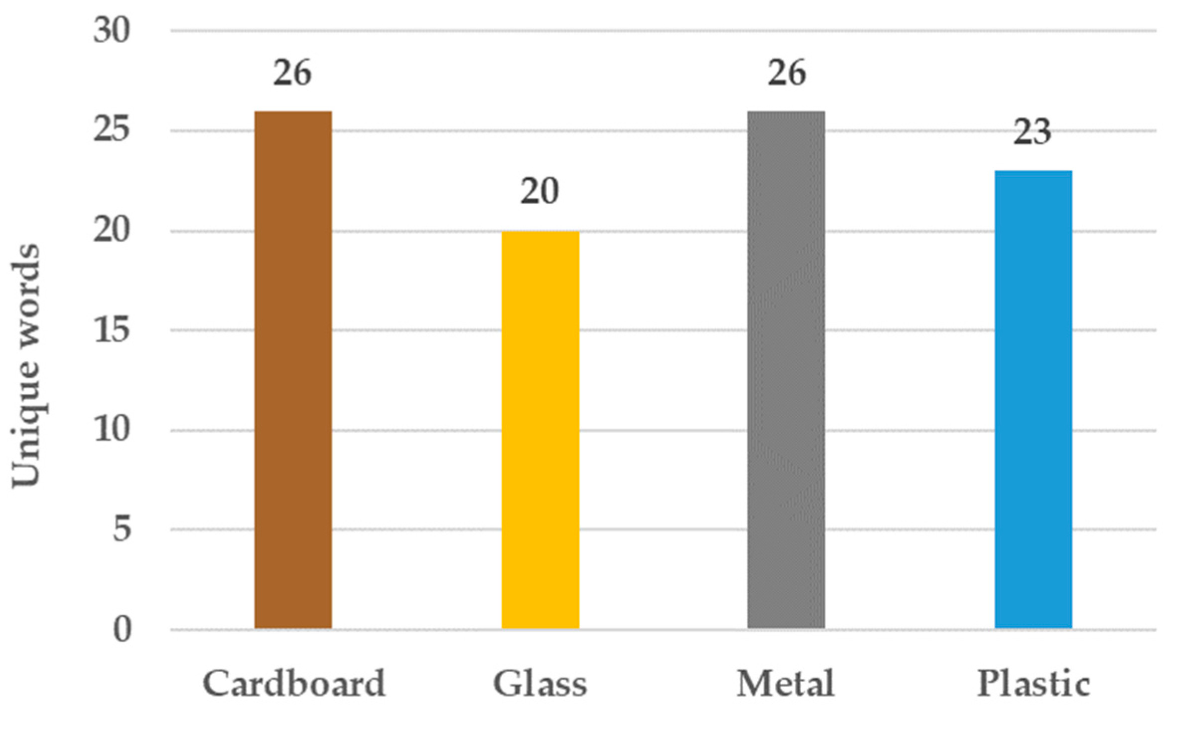
Figure 8 presents a statistical demonstration of the training dataset obtained after applying GVAS. In this figure, the unique words that ensure differentiation between categories have been retained. This demonstration ensures the CWSM’s ability to distinguish between categories correctly. Figure 9 shows the unique words identified for each category in the validation set that are also found in the training set. The authors note that the training set may also contain words not found in the training set, but they rely on the description containing other words that allow differentiation, so it does not rely exclusively on that word. In Figure 8, statistics were calculated regarding the uniqueness of words that allow differentiation between categories in the analysis of descriptions generated by GVAS for the 1000 images. This GVAS model ensures the textual extraction of image descriptions from the training set of 1000 elements. To visualize this statistic in Figure 8, common descriptive elements identified in two or more categories were removed. For example, the word transparency is recognized in the plastic and glass categories. The word’s presence in both categories causes the model to become confused in the second training layer. However, unique elements ensure a clear distinction between categories, alongside these common elements that irrevocably exclude other classes. Narrowing the domain of classes and subsequently firmly distinguishing them through distinctive elements allows the model to identify the class to which an object belongs accurately.

4.1. Testing Azure Custom Vision Service

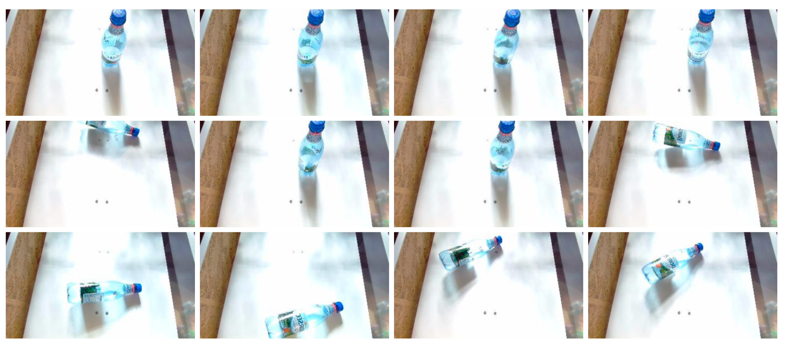
Figure 10 shows a screenshot of a plastic bottle from the training dataset. Thus, the bottle is placed in different positions on the sorting flap and oriented at various angles. The fact that a multitude of images must be acquired for each object, capturing it in various scenarios, represents a major drawback of the service used by ACVS. In real life, it is impossible to acquire all the features for all the objects in the world to perform correct training. Therefore, the model must be able to generalize and distinguish between objects based on this generalization, which must be distinctive between categories.

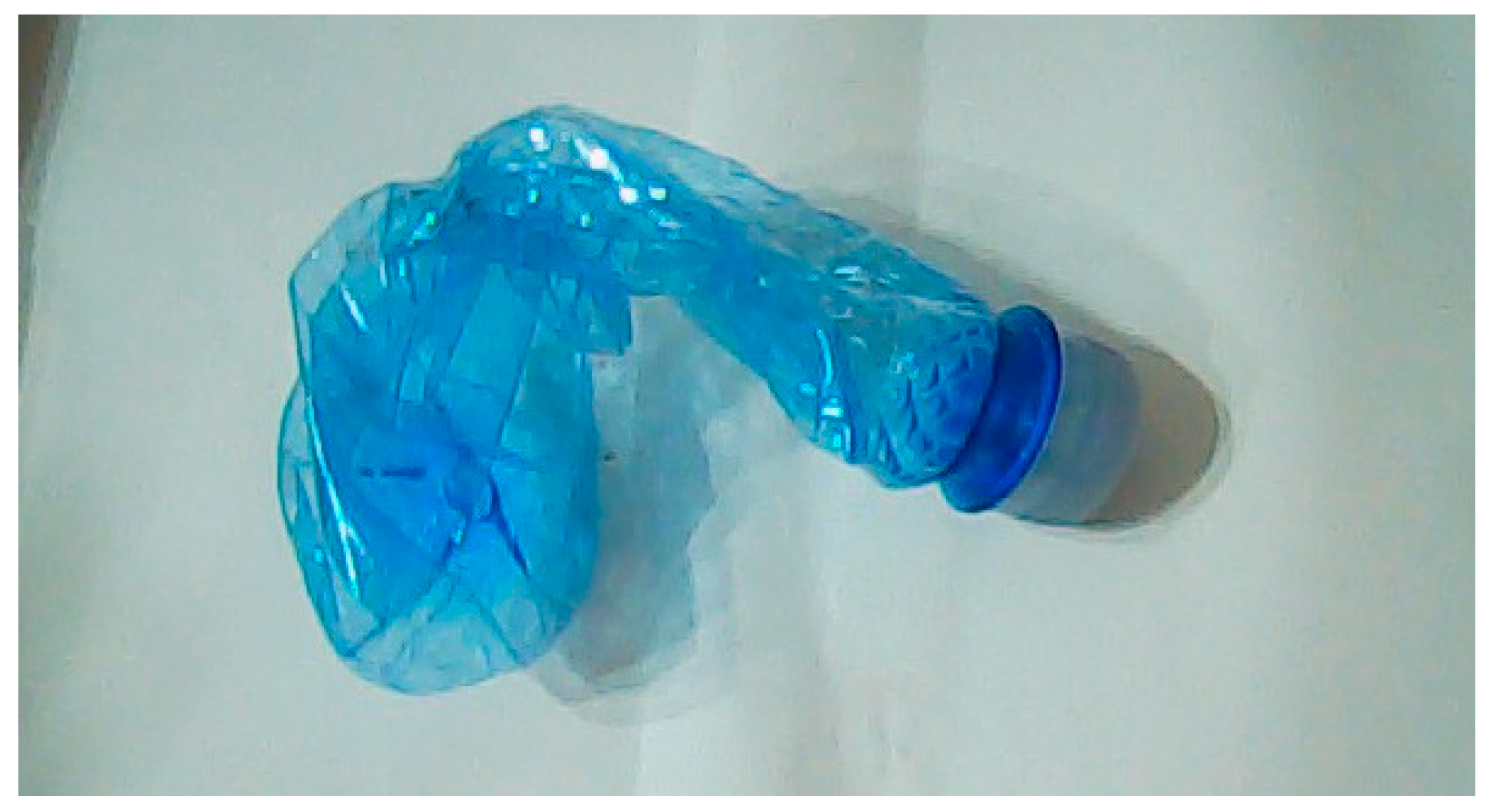
Figure 11 shows a plastic bottle that is flattened. Suppose this image is sent to ACVS by placing the bottle in different positions and oriented at various angles (similar to the images in Figure 10). In that case, ACVS will not have the ability to identify that it is the same bottle.

To recognize a flattened plastic bottle, ACVS needs to be trained with numerous bottles in different positions and at various angles. Moreover, using a flattened plastic bottle of a different color requires a separate dataset during the training phase to successfully perform the recognition. This behavior suggests the low capacity of the service regarding generalization, meaning the ability to extrapolate the features of objects identified during training. The degree of flattening of the bottle is another factor that affects the recognition capability. Essentially, if the bottle is flattened differently, there is a chance it will not be recognized correctly. Furthermore, another object from a different sorting category could be misidentified as a flattened plastic bottle if it shares more similarities with that object than with the training images in the plastic class.

Table 2. Performance parameters for each category of ACVS.

Category	Accuracy (%)	Precision (%)	Recall (%)	F1-Score (%)
Cardboard	99.00	97.06	99.00	98.02
Glass	94.25	82.91	97.00	89.40
Metal	96.50	89.09	98.00	93.33
Plastic	90.75	94.37	67.00	78.36
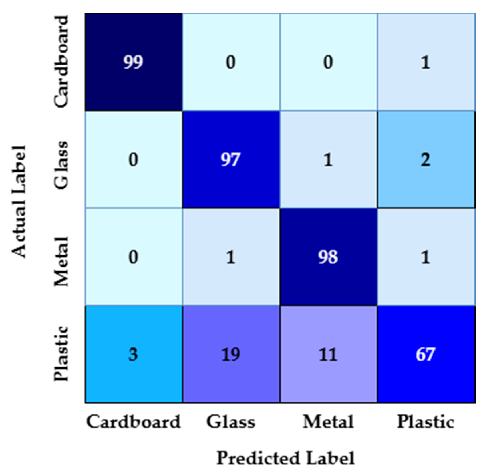
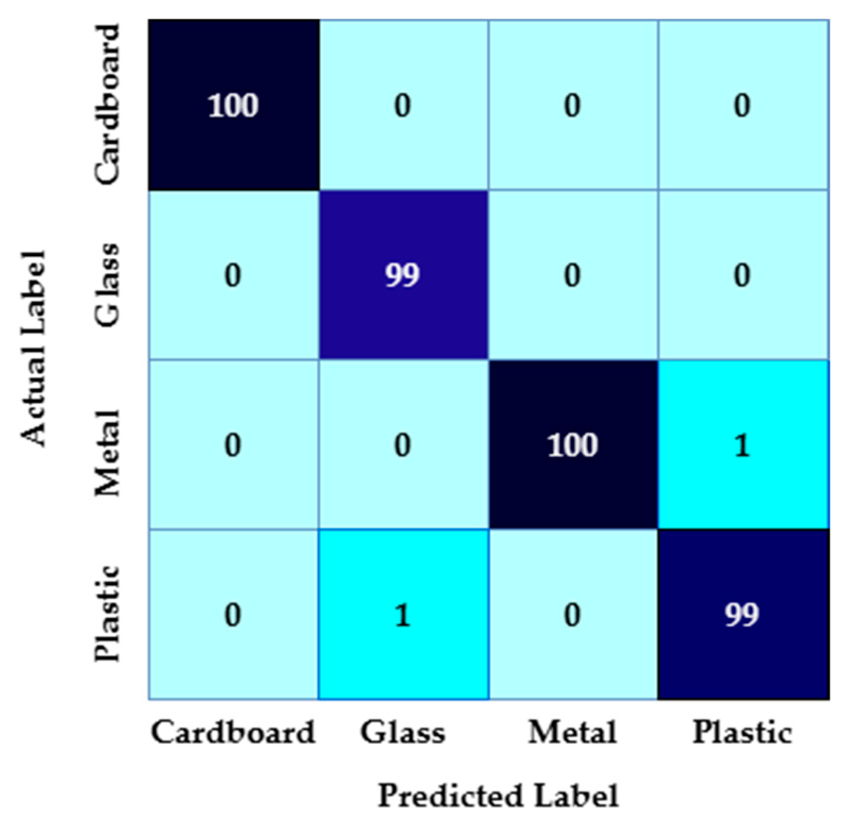
Total	95.13	90.86	90.25	90.55

presents the results for 400 unseen images after the training (which involved 1000 images, 250 for each category). Out of the one hundred tests for metal, ninety-eight were recognized as metal, one was identified as glass, and one was identified as plastic. For the cardboard tests, ninety-nine of one hundred were recognized as cardboard, while one was recognized as plastic. Ninety-seven were correctly identified for the glass tests, while two were identified as plastic and one as metal. For the plastic tests, sixty-seven were identified as plastic, eleven as metal, nineteen as glass, and three as cardboard (Figure 12).

ACVS demonstrates moderate performance in classifying a never-seen object from a category. The confusion matrix is presented in Figure 12. The precision is calculated at 90.86%. In this context, the ACVS model avoids many false positives (FPs), meaning that it is often correct when it predicts a certain category. The accuracy of ACVS for never-before-seen objects is 95.13%.

4.2. Testing the Custom Waste Sorting Model

The CWSM is a hybrid model incorporating a first component for object description and a second component including a classification model based on the previous description. While the first component is an automated process performed by GVAS, an external service, the second component is a local service performed by the Microsoft ML.NET tool. The second component is locally trained and evaluated using five algorithms. 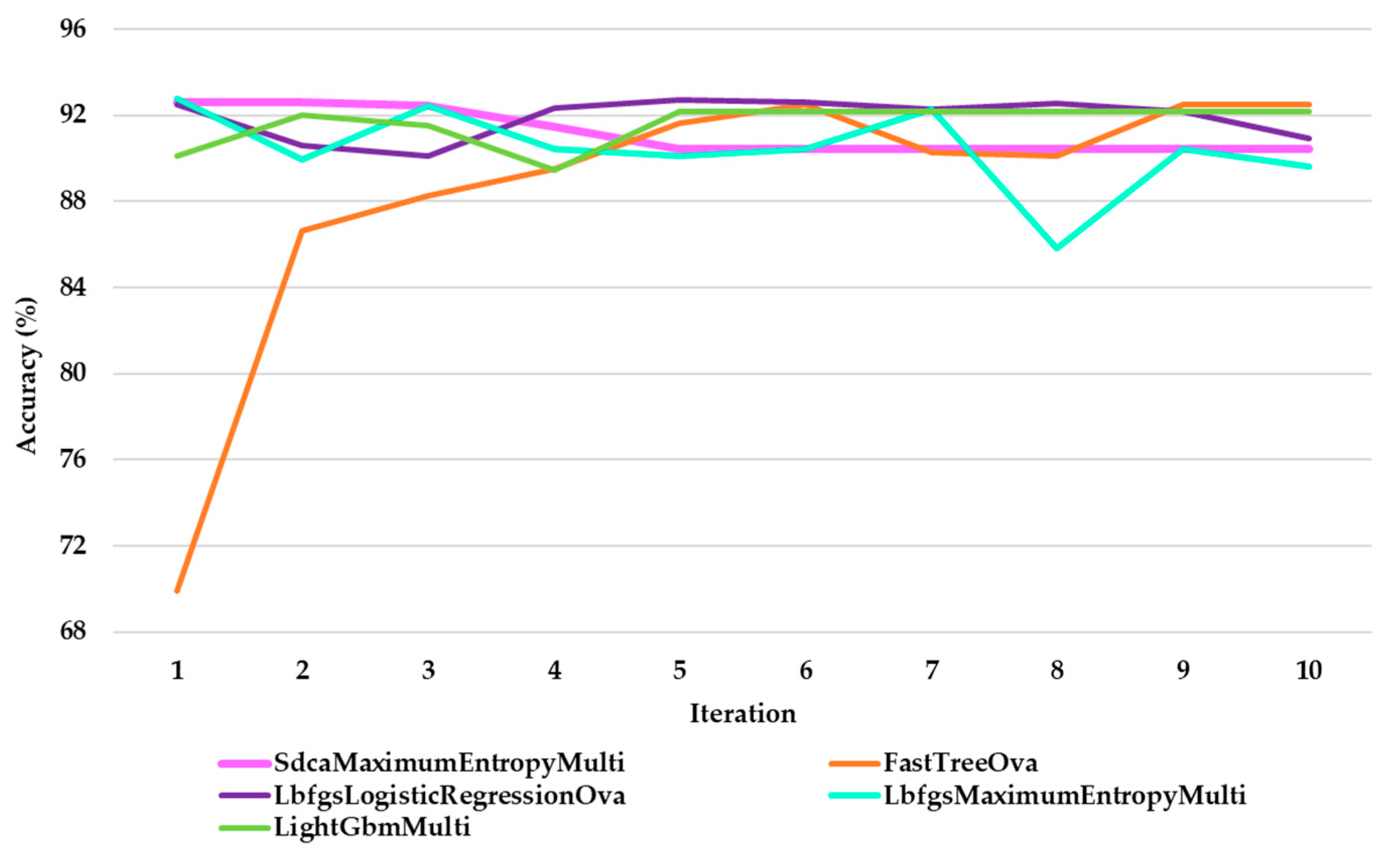Figure 13 presents the accuracy for all evaluated algorithms through multiple iterations. Thus, the superiority of LbfgsMaximumEntropyMulti is visible in Figure 13. This algorithm calculated an accuracy of 92.79% for the classification, indicating that the model predicts most of the analyzed categories.

The LbfgsMaximumEntropy algorithm represents a variant of multiclass logistic regression based on Maximum Entropy. This method is optimized using the Limited-memory Broyden–Fletcher–Goldfarb–Shanno (L-BFGS) algorithm. It is suitable for text classification because it maximizes the probability of an object belonging to one of the defined classes: plastic, glass, metal, and paper.

LbfgsMaximumEntropy provided the best results for text classification because this algorithm excels in solving multiclass problems. Unlike standard algorithms, such as the SVM, which is more suitable for binary classification and requires a one-versus-one approach, LbfgsMaximumEntropy uses reduced complexity, facilitating integration into real-time decision making. Random forest, one of the most analyzed algorithms in the specialized literature, is not ideal for textual data because it works better with discrete features than with continuous representations, such as text vectors. LbfgsMaximumEntropy maximizes the probability of belonging to a class, converges quickly due to L-BFGS, and automatically adjusts through L1/L2 regularizations, preventing overfitting. Therefore, LbfgsMaximumEntropy does not have the architecture of a classical neural network with layers. However, it uses specific hyperparameters for training, whose values are set as follows:

• The L1 regression parameter (Lasso) is set to 5.20%. This controls the sparsity of the model, forcing some coefficients to be 0 to reduce model complexity;
• The L2 regression parameter (Ridge) is set to 18.75%. This parameter adds an extra penalty for large coefficients, preventing overfitting.

Since the LbfgsMaximumEntropy algorithm uses L-BFGS optimization, which automatically adjusts learning steps for fast convergence, it does not require the specific parameters of a neural network.

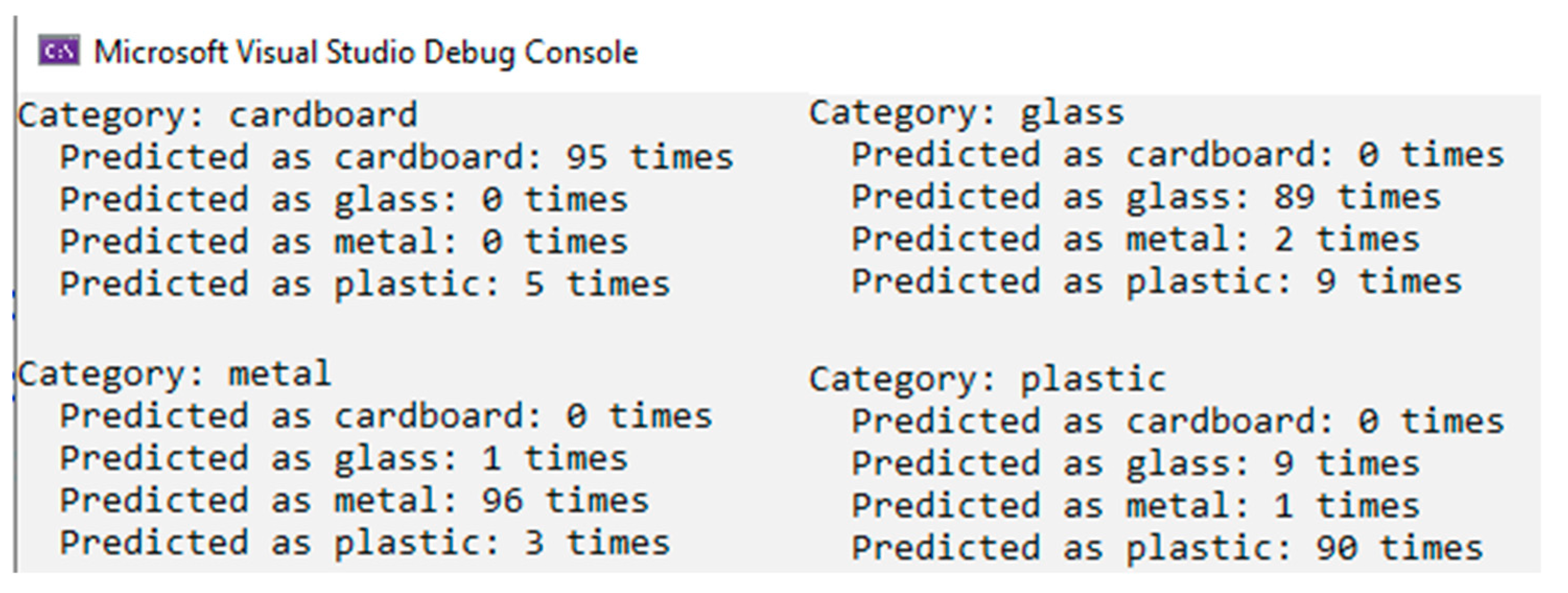
The CWSM is examined using the same unseen object for the training dataset. The script execution using the ML.NET tool, C# programming language, and Visual Studio development environment is presented in Figure 14. The results are identified as follows (Figure 14):

• Cardboard recognition achieves accuracy at 98.75%. This result reflects that the CWSM can recognize cardboard objects. This performance suggests that the defining characteristics of the cardboard class are well represented in the training data;
• The glass category has an accuracy of 94.75%. The CWSM performs reasonably well, but there is room for improvement in handling more diverse or challenging glass-related features. This score reflects the confusion with the plastic category;
• Metal is identified with a 98.25% accuracy rate, showcasing strong performance in identifying metallic objects;
• Plastic has approximately the same accuracy as the glass category. The accuracy for plastic stands at 93.25%, indicating poor performance.

Table 3. Performance parameters for each category of the CWSM.

Category	Accuracy (%)	Precision (%)	Recall (%)	F1-Score (%)
Cardboard	98.75	95.00	100	97.44
Glass	94.75	89.00	89.90	89.45
Metal	98.25	96.00	96.97	96.48
Plastic	93.25	90.00	84.11	86.96
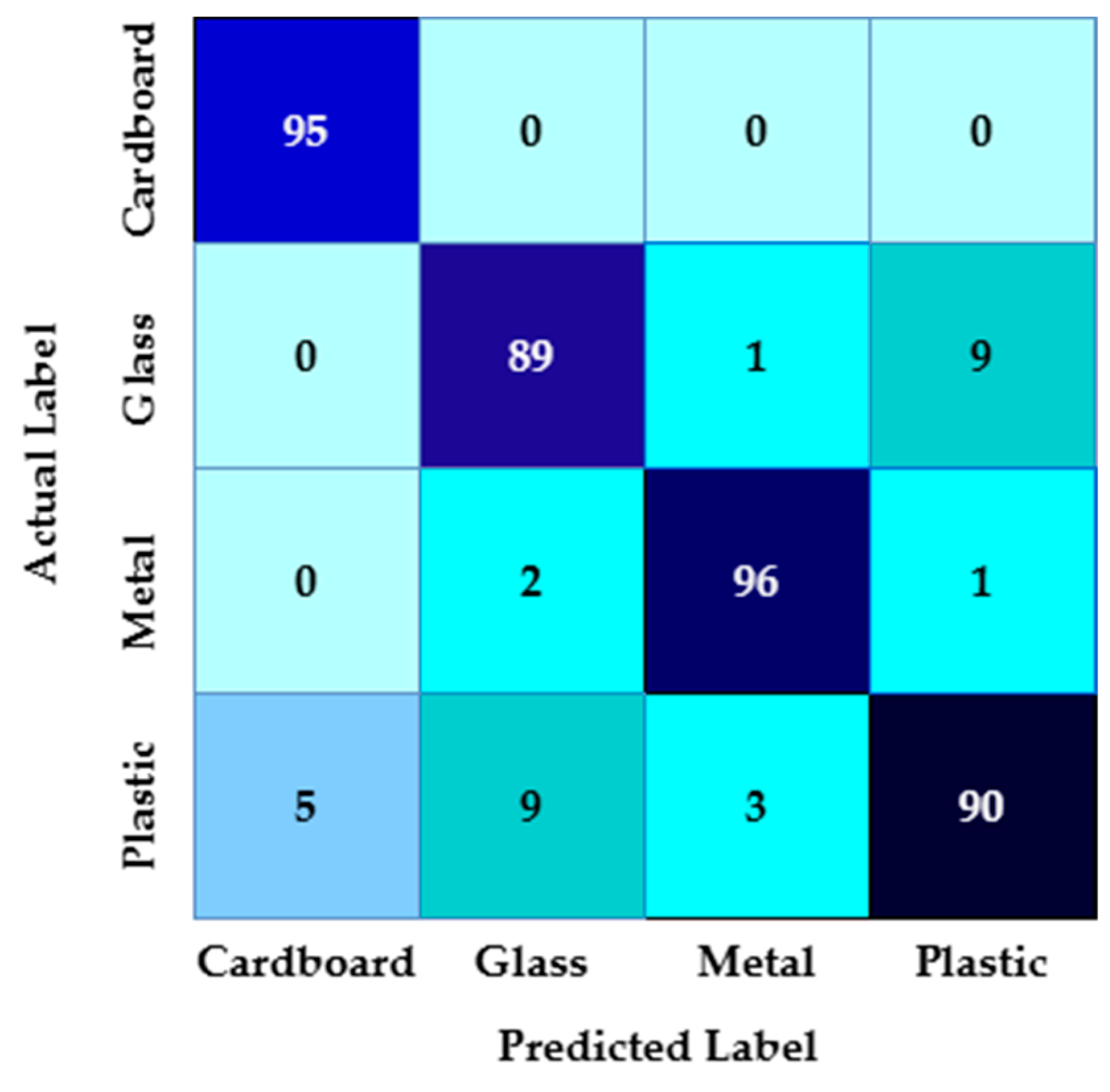
Total	96.25	92.50	92.75	92.62

presents the performance parameters for each waste category of the CWSM before applying the WCCS. The CWSM’s total accuracy is approximately 96.25%, which indicates its high performance. The confusion matrix presented in Figure 15 shows that cardboard has ninety-five true positives, and zero are misclassified. Glass has eighty-nine true positives; one is misclassified as metal and nine are misclassified as plastic. Metal has ninety-six true positives; two are misclassified as glass and one is misclassified as plastic. Plastic shows ninety true positives; five are misclassified as cardboard, nine are misclassified as glass, and three are misclassified as metal.

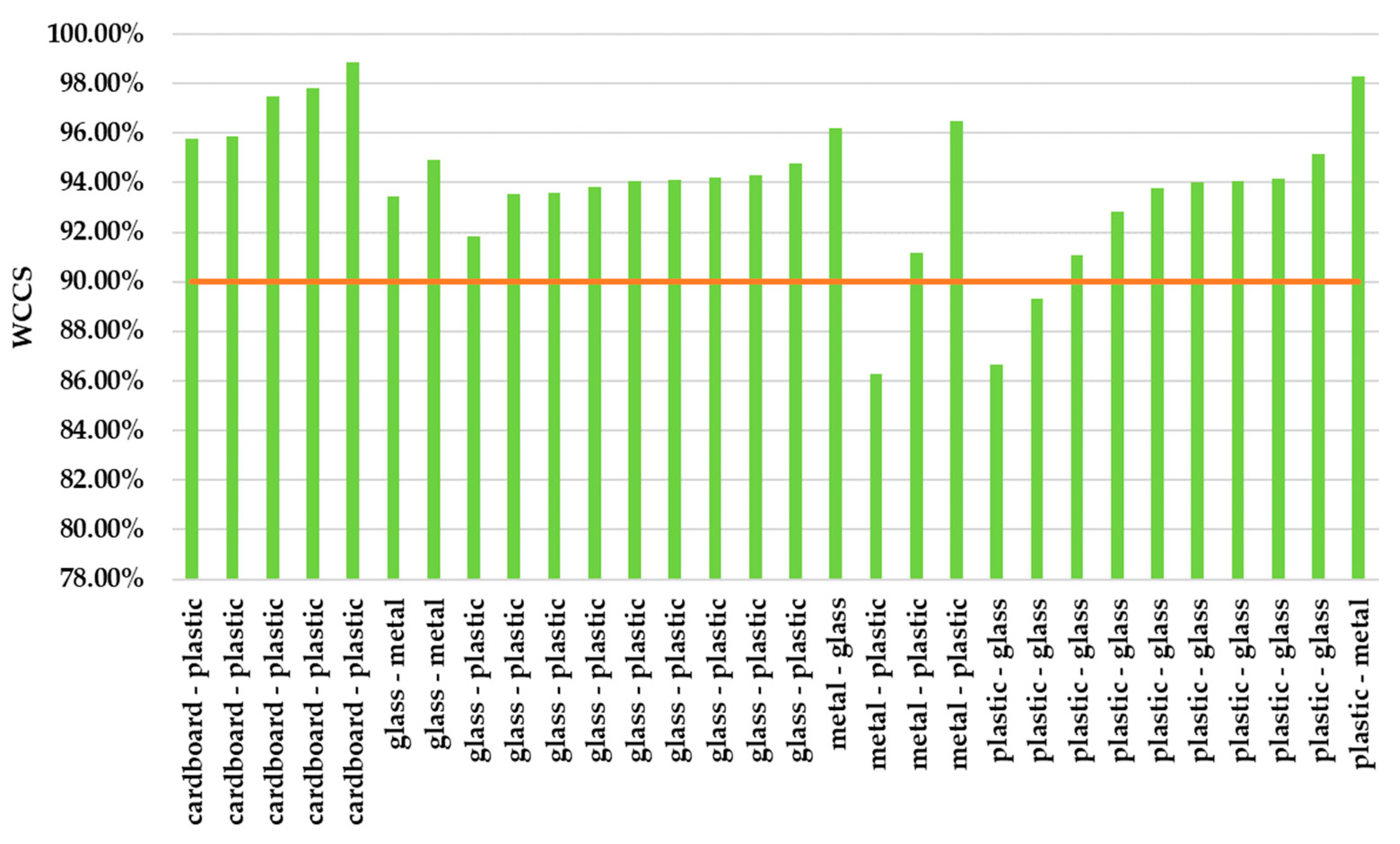
For the CWSM, we have imposed a 90% threshold of the WCCS (the red horizontal line in Figure 16). Suppose that when the WCCS level is higher than 90%, additional inspection is needed, such as in the cases in Figure 16. Thus, the thirty misclassified elements are represented, and it is seen that after applying the WCCS, only two elements will remain misclassified. Therefore, Figure 17 presents the confusion matrix obtained after applying the WCCS.

Table 4. Performance parameters for each category of the CWSM after applying the WCCS.

Category	Accuracy (%)	Precision (%)	Recall (%)	F1-Score (%)
Cardboard	100	100	100	100
Glass	99.75	99.00	100	99.50
Metal	99.75	100	99.01	99.50
Plastic	99.50	99.00	99.00	99.00
Total	99.75	99.50	99.50	99.50

presents the performance parameters after applying the WCCS.

The results in Table 4 show a significant improvement in the performance metrics for all four categories. Thus, the overall accuracy obtained for the CWSM after applying the WCSS for all four categories is 99.75%, with a precision of 99.50%, a recall of 99.50%, and an F₁-Score of 99.50%. This is because when the CWSM does not have a sufficiently high confidence level in classifying an object, it relies on the user’s final decision.

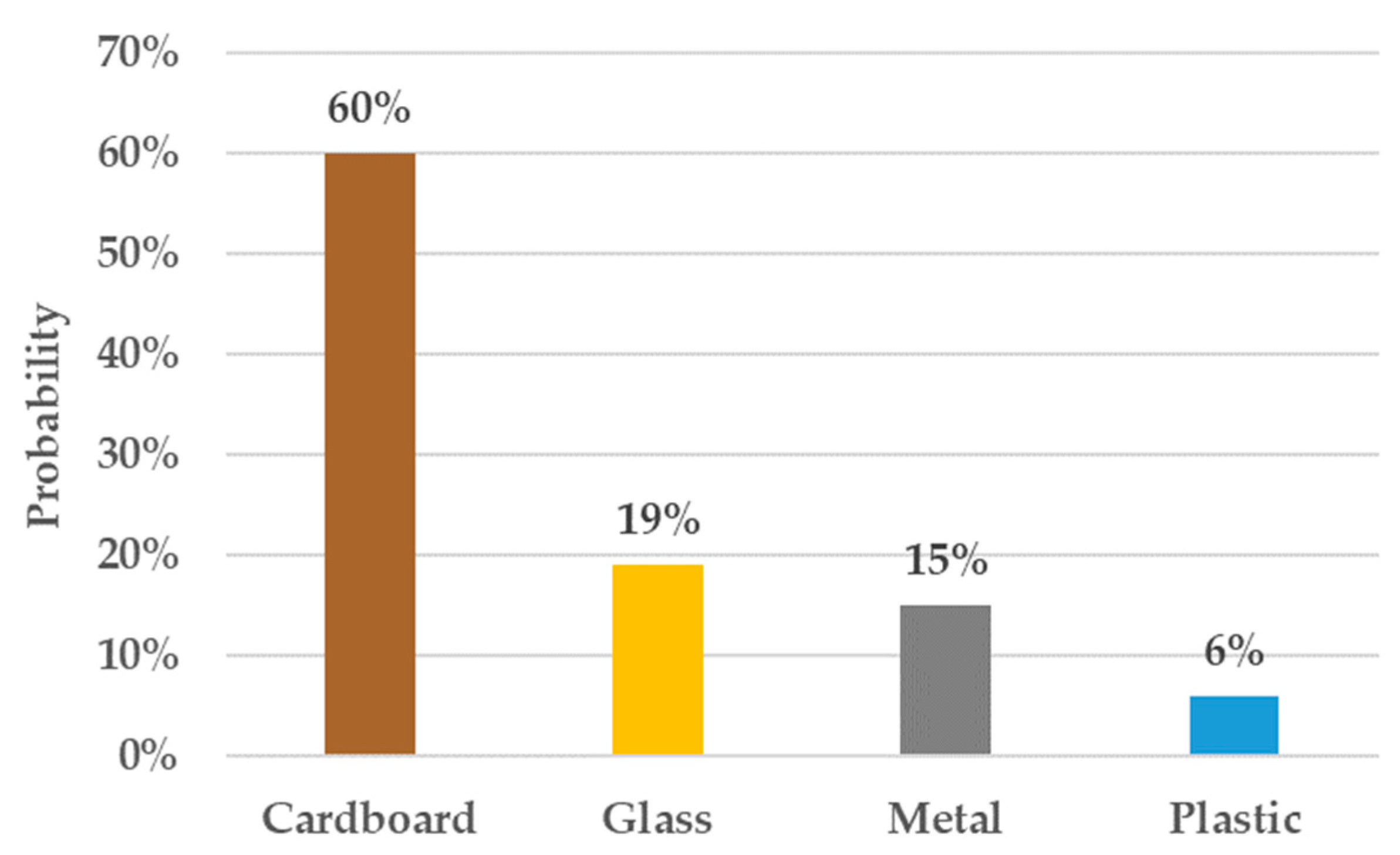
In what follows, we detail the computation of the WCCS for two scenarios. The first scenario presents when the CWSM correctly identifies the object waste category. We analyze cardboard objects, identified as cardboard, with the probabilities provided by GVAS (Figure 18).

Because there are no multiple identifications for the same class, the mean probability μ is 0.25. The variance is 0.043 as follows:

$$Variance={\displaystyle \frac{{(0.60-0.25)}^2+{(0.19-0.25)}^2+{(0.15-0.25)}^2+{(0.06-0.25)}^2}{4}}=0.043$$

Using this variance value, the WCSS is as follows:

$$WCCS={\displaystyle \frac{0.60+0.19+0.15+0.06}{1+0.043}}\times 100=0.959\times 100=95.9\%$$

This value indicates the necessity of checking manually whether the CWSM made a valid identification.

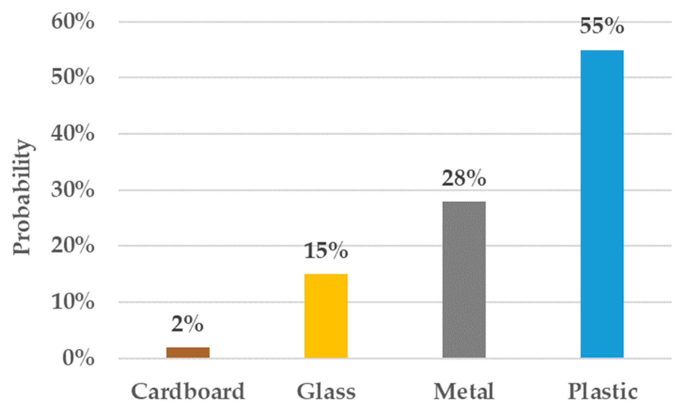
The second scenario corresponds to an incorrect evaluation. We evaluated a glass object that was identified as plastic (Figure 19).

The mean probability is 0.25, and the variance is calculated at 0.03. The WCCS of 96.3% reflects high confidence in the dominant category (plastic, 55%), with some probability spread indicating uncertainty.

Exceeding the value of 0.90 indicates particular attention to identification. It does not mean an incorrect classification. It rather highlights a degree of uncertainty regarding the way the class was identified. Mathematically, this threshold value indicates a boundary where the CWSM’s confidence becomes less evenly distributed across categories, resulting in a higher concentration of probability in one or more specific classes.

The threshold of 0.90 is derived to balance confidence with variability (measured as variance). A WCCS above this threshold suggests that the classifier has a dominant waste category. At the same time, it shows inconsistency in distributing probabilities across other potential waste categories. Exceeding the 90% value points out ambiguities in the feature space and data patterns that challenge the CWSM’s decision-making process.

4.3. Architectural Differences and Real-Time Performance Comparision

ACVS is a pre-trained service configured for image classification. It uses a CNN to categorize an image into a specific category. The programmer declares these categories, but the networks are not customized, except by manually adding image labels. The ACVS service automatically processes distinctive features between images belonging to different categories.

Table 5. Key Comparative elements between ACVS and the CWSM.

Metric	ACVS	CWSM
Classification type	CNN	Hybrid
Methodology	Pattern identification	Text feature extraction
Object processing	Key pattern distinctive category extraction	Features comparison among categories
Flexibility	Extended training dataset	High generalization on a reduced dataset

presents the key comparative elements between the two models.

In contrast to ACVS, the CWSM has a hybrid approach. The first stage analyzes the current image and performs descriptive extraction through GVAS. The description consists of semantic characteristics. In the second stage, the CWSM processes and assigns the textual description to one of the four defect categories in the training phase and then predicts the category based on the validation description.

ACVS is an architecture suitable for applications specific to controlled environments, i.e., when the testing images are similar to the training ones. A concrete example is the one disseminated by the authors in [58], where defect detection at the level of gear wheels is performed. In this case, the images for identifying the defect significantly differ from the training images. On the other hand, in the case of a basket, the images have too much variability. This variability causes a system to be unable to generalize to such an extent that it can accurately identify all objects.

ACVS trains using the following procedures:

• Load all images;
• Mark in all images the area containing the object and associate the label with the corresponding category of the object;
• Train the model.

Analyzing these steps of the training procedure reveals that the programmer lacks flexibility in developing the model. On the other hand, this procedure is advantageous from the perspective of relieving the programmer of the burden of implementing image processing mechanisms and from the perspective of the Microsoft service’s capability for auto-tuning model parameters to generate the best metrics.

GVAS has a superior generalization capability to ACVS, as it uses semantic descriptions rather than pixel-level analyses. Unlike ACVS, GVAS is more efficient in real-time processing because it does not require an extensive database of images for comparison. Text-based processing is much faster due to reduced time–space complexity. Moreover, the CWSM, including GVAS as a first layer, has higher accuracy than ACVS, even for unknown objects, as it classifies based on descriptive characteristics, not just visual ones. This behavior demonstrates the superior generalization ability of the CWSM compared to ACVS. One final comparative advantage is the enhanced adjustability of the GVAS model in terms of optimizations. This is possible by improving the labels provided by GVAS, given that the first component of the model is text based.

Therefore, the CWSM performs better in real-time applications due to its reduced inference time, high generalization capability, and ability to improve under varying conditions. ACVS must compare each provided image with the training dataset. This complex process makes the ACVS model slow and dependent on cloud infrastructure. In contrast, the CWSM classifies based on semantic characteristics, resulting in reduced processing time.

The ACVS model cannot recognize objects it did not see during training. On the other hand, the CWSM analyzes object descriptions, allowing it to generalize better and identify new categories without additional training.

The image-level analysis makes ACVS sensitive to lighting, angle, and image quality variations, which affect classification. The CWSM, using textual labels, reduces the impact of these factors, ensuring that the model’s accuracy remains consistent in varied environments.

4.4. ANOVA Performance Comparison

The TrashNet model [60] analyzes the accuracy for the same categories the CSWM employs. The comparative data are presented in

Table 6. Accuracy comparison between the TrashNet model and the CWSM.

Category	TrashNet (%)	CWSM (%)
Cardboard	97.6	100
Glass	94.4	99.75
Metal	88.7	99.75
Plastic	81.3	99.50
Total	91.7	99.75

. The analysis of variance (ANOVA) comparative model is provided compared to the TrashNet model to maintain the same evaluation categories.

The defined ANOVA hypotheses are as follows:

• Null Hypothesis (H₀). The mean accuracy difference between the models across categories is not relevant;
• Alternative Hypothesis (H₁). The mean accuracy difference between the models across categories is relevant.

The mean of TrashNet and the CWSM are computed as follows:

$${Mean}_{TrashNet}={\displaystyle \frac{88.7+81.3+97.6+94.4}{4}}=90.5$$

$${Mean}_{CWSM}={\displaystyle \frac{99.75+99.50+100.00+99.75}{4}}=99.75$$

The overall mean is as follows:

$${Mean}_{Overall}={\displaystyle \frac{88.7+81.3+97.6+94.4+99.75+99.50+100.00+99.75}{8}}=95.12$$

Next, we compute sums of squares using Equation (9) [61] as follows:

$$SSB=n_1{(\overline{x_1}-\overline{x})}^2+n_2{(\overline{x_2}-\overline{x})}^2,$$

(9)

where

SSB is the Sum of Squares;

n₁ is the number of observations in TrashNet;

n₂ is the number of observations in the CWSM;

$\overline{x_1}$ is the mean of TrashNet;

$\overline{x_2}$ is the mean of the CWSM;

$\overline{x}$ is the overall mean.

By applying Equation (9), the following is obtained:

$$SSB=4{(90.5-95.12)}^2+4{(99.75-95.12)}^2=85.36+85.36=170.72$$

Next, we calculate the Within-Groups Sum of Squares (SSW) using Equation (10) [61] as follows:

$$SSW={\sum }_{i=1}^4{(\overline{X_i}-\overline{x_g})}^2,$$

(10)

where

SSW is the Within-Groups Sum of Squares;

X_i is the accuracy of the corresponding category for the analyzed model;

$\overline{x_g}$ is the mean of the analyzed model.

By applying Equation (10), the following are obtained:

$${SSW}_{TrashNet}={(97.6-90.5)}^2+{(94.4-90.5)}^2+{(88.7-90.5)}^2+{(81.3-90.5)}^2=153.5$$

$${SSW}_{CWSM}={(100-99.75)}^2+{(99.75-99.75)}^2+{(99.5-99.75)}^2+{(99.75-99.75)}^2=0.125$$

$$SSW=153.5+0.125=153.62$$

Next, we calculate the Between-Groups Degrees of Freedom (dfB), where the number of groups is g = 2 using Equation (11), and the Within-Groups Degrees of Freedom (dfW), where a total number of observations is k = 8 using Equation (12) [61].

$$dfB=g-1=2-1=1$$

(11)

$$dfW=k-g=8-2=6$$

(12)

Next, we calculate the Between-Groups Mean Square (MSB) and Within-Groups Mean Square (MSW) using Equations (13) and (14) [61] as follows:

$$MSB={\displaystyle \frac{SSB}{dfB}}={\displaystyle \frac{170.72}{1}}=170.72$$

(13)

$$MSW={\displaystyle \frac{SSW}{dfW}}={\displaystyle \frac{153.62}{6}}=25.60$$

(14)

We calculate the F-statistic using Equation (15) [61] and determine the critical value for F at a significance level of 0.05 with dfB = 1 and dfW = 6. We identify the critical value at 5.99 using the Excel function FINV(0.05, 1, 6), where 0.5 is the significance level, 1 is the dfB, and 6 is the dfW. Since the calculated F = 6.668 > 5.99, we reject the null hypothesis.

$$F={\displaystyle \frac{MSB}{MSW}}={\displaystyle \frac{170.72}{25.60}}=6.668$$

(15)

By rejecting the null hypothesis, it is accepted that the CWSM yields superior results compared to similar models in the literature, as evidenced by the comparison with the TrashNet model. The ANOVA statistical analysis validates this comparison.

5. Discussion

This research analyses two object identification models and their classification into cardboard, glass, plastic, and metal categories. The biggest issue with these classifications is the distinction between glass and plastic. The research shows that although the ACVS model has high accuracy on the trained data, it demonstrates a value of 95.13% in real-time applications, which means 5% of objects are deployed in the wrong compartment.

The paper also analyses the issue of the number of images used in training the model. From the tests, it is found that an increase in the number of images for a specific waste category can destabilize the model’s accuracy to the detriment of others. Also, from the tests, it was found that some classes, such as glass and plastic, share common characteristics that make it impossible to distinguish between the two classes. Moreover, adding additional images for these two categories does not solve the problem, as the model becomes even more confused in the distinction, becoming overestimated. Conversely, using too few images will cause the model to be undertrained.

A second model, the CWSM, which had an accuracy of 96.25% before the proposed WCCS, has demonstrated real-time usability by increasing the accuracy to 99.75% after applying the indicator. The CWSM is designed through descriptive identification of the object in the image, and then the category is identified through a second model. Initially, the description is obtained using the GVAS model, which analyses the object at the image processing level. Then, the CWSM is used, a custom model based on predicates and thus text-level processing. The algorithm used by the CWSM is LbfgsMaximumEntropyMulti, which achieved an accuracy of 92.79% during training. Furthermore, the model is evaluated through a unique tool specially designed for this type of classification, specifically for this research. This indicator, the WCCS, varies between 84.2% and 100%. A value of 84.2% indicates a certain classification in a specific category, with no doubts regarding allocating to the class. On the opposite side, a value of 100% indicates an uncertain capacity of the CWSM. RBin uses the CWSM in residential waste sorting.

Several studies have been analyzed in the specialized literature that aim to classify waste automatically. The paper by Bobulski and Piatkowski [62] presents the WaDaBa model for the classification of plastic waste, achieving an accuracy of 87.44%. The paper by Yuan and Liu [60] presents the TrashNet prototype, which achieved an accuracy of over 90%. In comparison with these models, the CWSM offers an innovative approach through the use of text-based labels. Classification algorithms enabled an accuracy of 99.75% to be reached. This value demonstrates, on the one hand, the superiority of the developed algorithm and, on the other hand, the feasibility of using textual descriptions instead of direct image-based training. The innovative aspect of this research lies in demonstrating the use of text descriptions extracted from images, as opposed to training directly on images. The TrashNet model used 2527 images, the WaDaBa model used 4000 images, and the CWSM used only 1000 images due to the superiority of the text extraction services. Using this reduced dataset in relation to the model’s high performance highlights the advantage of this approach.

The research highlights the importance of developing a custom model based on the description of the identified object. For the data engineer, using models that utilize unknown features makes pattern management unpredictable.

The paper outlines that the model based on ACVS cannot be used in practice. At the same time, GVAS was used to build the customized model further, representing a successful formula. Also, this research underlines that the theory stating that 75% of the data is used for training and the remaining 25% for model validation does not demonstrate the possibility of practical use. The research demonstrates the superiority of using a model that is based on identifying common features of objects belonging to the same class but distinguishes them from other categories. The paper also demonstrates that the processing techniques implemented by pre-implemented AI models are not sufficient for use in real-time applications, as they cannot extrapolate for objects that have never been used before. Furthermore, the custom algorithms implemented must also contain mechanisms to prevent situations involving overlapping common features between classes, such as the case of glass–plastic. This research materialized these mechanisms through the WCCS indicator, demonstrating the ability to identify these exceptional situations.

The WCCS indicator proposed in this study assesses the confidence in classifying an object. Unlike other model performance evaluation methods, the WCCS penalizes model uncertainty. Compared to traditional performance evaluation methods, the WCCS has the following advantages.

Unlike precision and recall, the WCCS incorporates probabilities for each category and normalizes the results. This approach provides a detailed view of performance per category, different from precision and recall, which do not offer insight into the model’s uncertainty regarding specific categories.

• The F₁-Score is another traditional metric for evaluating model performance. Even if the model has a good F1 score, its classifications may still be uncertain. Unlike the F₁-Score, if the model is indecisive between two categories, the WCCS establishes an additional degree of confidence;
• The Brier score is another metric that measures how well a model’s probabilities are calibrated. It does not differentiate between a slightly uncertain model and a completely wrong one. Unlike the Brier score, the WCCS heavily penalizes uncertainty and over-confidence in incorrect predictions.
• Entropy is another tool for measuring a model’s probability distribution. It does not normalize the results based on the dominant category. In contrast, the WCCS introduces normalization based on category importance and probability variation.

The WCCS, together with standard model evaluation metrics, provides an advanced means of assessment compared to traditional metrics.

The paper analyses current reference technologies in the AI field through the Custom Vision services implemented by Azure Custom Vision and Google. The authors believe these two services offer features that cannot be replaced by custom development with a few programmers. Still, they have limited capabilities if not integrated into a customized solution, like the one proposed in this paper.

The comparative analysis reveals the evident limitations of ACVS, which requires a large volume of training data. GVAS demonstrates superiority in the context of being integrated as part of the CWSM in the classification problem. The research limitations are given by the number of images used in training and testing. Even if we employed 1000 images for training and 400 images for testing from all four waste categories, it is impossible to test all types of waste (because they have particular shapes, colors, sizes, etc., even in the same waste category) that are produced worldwide and to acquire images from different angles, light types, brightness levels, and shadows.

RBin’s internet connection influences the processing speed of the CWSM since the model uses GVAS for object labeling at the image level. In the case of a slow connection, the classification process may experience delays. Still, these do not affect the practical use of the system, as user interaction with the waste bin does not require immediate real-time processing. System latency is not an issue because users do not dispose of waste at speeds exceeding a computing system’s processing capacity. Even in high volumes of waste scenarios, the classification process is fast enough to meet user requirements. Regarding scalability, the CWSM can handle large datasets because it uses text-level processing faster than pixel-to-pixel comparative analyses. Adjusting the WCCS weights modifies the model’s performance based on the scenario and the diversity of the dataset.

The scientific value of the RBin prototype lies in the impact that cloud technologies, along with ML methods, have on everyday life, an aspect demonstrated through their application in the field of waste classification. The demonstration was possible by developing a hybrid model, combining automatic object labeling via GVAS and its classification using ML.NET. The model performing the actual classification is based on LbfgsMaximumEntropyMulti. The functionality of the RBin prototype demonstrates the superior capabilities offered by custom-made solutions, which also integrate pre-trained technologies with applicability in recognizing categories of waste (cardboard, glass, metal, plastic). The proposed model generates the WCCS that enhances the reliability of classification decisions. This score manages situations where multiple categories may be assigned to the same object, reducing the risk of incorrect classification. The impact on the field of automated recycling comes from the improvement in classification accuracy, reaching 99.75% after applying the WCCS.

6. Conclusions

The paper analyses key topics in the specialized literature on sorting and recycling. The research follows two major directions: hardware-based approaches that use sensors and software-based approaches that use AI models trained to distinguish between different categories of objects specific to sorting classes. Subsequently, this paper proposes a configuration that allows for the creation of low-cost hardware for an intelligent bin, RBin, which enables residential sorting by classifying objects into cardboard, glass, plastic, and metal categories. The prototype used was made for the sum of 563 EUR. The setup includes the latest version of the Raspberry Pi device. At the same time, a display for showing messages is added to the setup, but it could be omitted for the commercial versions, having, as a result, a cost reduction.

After the assembly was completed, tests were performed by sending commands, and it was realized that the prototype could be 100% functional if it used an appropriate object classification algorithm, demonstrating the assembly’s feasibility. ACVS was trained using 1000 images (250 for each category) and evaluated using 400 images (100 for each category).

In the following, the research continues with the issue of identifying the optimal number of images for training an AI service using ML. Initially, ACVS was evaluated by employing 100 images for each category. The second test involved an imbalanced number of images for each category, and the result demonstrated poor values in metrics performance indicators. The last test trained the model using 250 images per category, containing objects with different characteristics and scenarios. The problem with this reporting was that it was demonstrated to be associated exclusively with the objects in the training set. In other words, the service cannot extrapolate for objects it has never seen before, meaning it cannot learn from the typical characteristics of trained objects. Therefore, the service can only learn from the attributes of trained objects. This approach is unsuitable for the sorting problem, which may include objects the service has never seen during the training stage. For these reasons, the research continues with reasoning that involves extracting standard features of the classes and being able to distinguish these classes based on features.

In what follows, GVAS extracted the features of the objects identified in the images. Thus, 1000 objects were analyzed, 250 for each category, and the same images were evaluated for the ACVS model. The output of this model is a label–description correlation in JSON format. Next, a custom model was developed based on predicates, i.e., text-level evaluations. The model used the LbfgsMaximumEntropyMulti algorithm. The ML.NET tool evaluated the five algorithms using 75% of the training-provided data for the training process and 25% for a comparative evaluation of the algorithms using the same training-provided data. The ratio of 75–25% is an internal setup of the ML.NET tool as a comparative measure among the evaluated algorithms. Again, 750 tests were used for training, uniformly distributed across the four analyzed classes, and the remaining 250 were used for internal first validation. Under these conditions, the CWSM achieved an accuracy of only 96.25%, which is considered sensible and superior to the previously developed ACVS model. Subsequently, a practical evaluation was performed on a sample of 400 images never seen before, 100 for each category. The CWSM’s accuracy is accounted for by the WCCS indicator, which, when values are higher than 90%, indicates potential insecurities of the CWSM and requires the assistance of a human operator to decide on the classification. This indicator allows the model to resolve the issue that arises from the inability of the classes’ common attributes to distinguish the objects being analyzed. The accuracy of the CWSM after applying the WCCS was 99.75%.

The general conclusions of the article focus on the inability of AI models to extract distinctive features when a large number of characteristics are involved based on images so that they can make extrapolations that allow them to identify objects they have never seen before. Customized models are necessary to perform such tasks, as demonstrated by the research presented in this article. Equally, choosing an optimal number of data that does not lead to underfitting or overfitting is an experimental matter that falls within the responsibility of the AI engineer. Additionally, using a customized indicator specific to the problem ensures the identification of cases not recognized by the service. The article demonstrates, through the prototype created at low costs and the uniqueness of the proposed CWSM, the superiority of customized models over pre-implemented services developed by companies such as Google LLC, Mountain View, CA, USA or Microsoft Corporation, Redmond, WA, USA.

Future research should integrate spectrometry sensors into RBin, which, in combination with the algorithm proposed in this paper, aim to achieve 100% accuracy in waste classification. New categories, such as food waste collection for compost production, are also being considered. The authors propose to investigate the possibility of integrating infrared spectroscopy to distinguish between different plastic, cardboard, and metal types, even when the objects are deformed or damaged. Additionally, X-ray fluorescence is another idea the authors wish to explore as a research direction for the rapid detection of metals. Integrating these sensors into RBin would represent a classification process that would eliminate confusion between visually similar materials. Moreover, developing a multimodal classification system is an important research direction the authors propose for improving RBin. This direction would enable a smart system capable of detecting the physical properties of waste (density, weight, recyclability) through IoT sensors. Furthermore, using ML technologies on edge devices (e.g., Raspberry Pi + AI accelerators) to classify waste without requiring a cloud connection would represent an evolutionary step for RBin, while transmitting data to a centralized waste management platform would allow for generating statistics about the types of collected waste and providing recommendations for improving recycling. This multimodal approach would enable better management in the recycling process and represents another research direction for the authors.