1. Introduction
With the acceleration of urbanisation and the diversification of residents’ travel needs, rail transit, as a high-capacity and high-efficiency urban transport mode, is playing an increasingly important role in easing urban traffic congestion and promoting coordinated regional sustainable development. At the same time, low-altitude economy, as an emerging mode of economic development, is gradually becoming an important force to promote urban economic growth and enhance the efficiency of urban management. Low-altitude economy not only involves new service forms such as drone delivery but also covers the demand for operating space for low-altitude vehicles, all of which bring new challenges and opportunities for urban built environment planning. Understanding and predicting rail traffic is crucial for optimising the allocation of public transport resources and improving operational efficiency and service quality. It is of great practical significance to clarify the relationship between built environment factors and ridership generation patterns and their influence mechanisms in order to optimise the planning layout of the rail transit system, improve operational efficiency, and ensure traffic safety. Therefore, this study takes the Shenzhen rail transit system as an example to explore the influence mechanism of built environment factors on ridership generation and distribution around stations, which will provide stronger theoretical support for the planning and effective management of urban public transportation systems and help realise a more intelligent and sustainable urban transportation optimisation scheme.
However, the factors affecting the ridership of rail transit are complex and diverse, including both internal factors of rail transit system, such as train frequency and service quality, and external built environment factors, such as land use pattern, population distribution, house price level, and layout of public service facilities. The existing studies on the impact of the built environment on rail transit ridership have primarily focused on linear models and spatial heterogeneity [
1,
2]. At the same time, these studies often overlook the nonlinear effects and the combined influence of internal and external environmental factors. Specifically, current research rarely considers the nonlinear effects of built environment factors in conjunction with spatial heterogeneity. Additionally, there is a lack of analysis using three-dimensional partial dependence plots.
Taking Shenzhen as an example, this paper applies the MGWR model and GBDT model based on the automatic fare collection (AFC) card swipe records and a variety of built environment variables to explore the impact of different built environment factors on the ridership in and out of the rail transit stations under different research perspectives. In order to consider the spatial heterogeneity, this study firstly adopts a multiscale geographically weighted regression (MGWR) model to visualise the spatial heterogeneity of built environment factors on inbound and outbound ridership. A machine learning model, Gradient Boosted Decision Tree (GBDT), was introduced with the aim of exploring the nonlinear relationship of the factors influencing ridership in rail transit. The marginal effects between the independent variables and the dependent variables are demonstrated through partial dependency diagrams (PDP), with the aim of comprehensively analysing the influence mechanism of rail transit ridership and providing scientific basis and technical support for relevant policy formulation.
This study aims to systematically investigate the nonlinear mechanism and spatial heterogeneity of built environment factors on the total ridership and inbound and outbound ridership of Shenzhen rail transit by integrating the multiscale geographically weighted regression (MGWR) model and the gradient boosting decision tree (GBDT) model, with a view to providing data-driven scientific basis for optimising the synergistic planning of the built environment and the rail transit and for enhancing the operational efficiency of the public transportation system. The study is aimed at providing data-driven scientific basis for optimising the synergistic planning of urban built environment and rail transit and enhancing the operational efficiency of public transportation system.
The innovations of this paper are as follows: (1) This study combines the spatial heterogeneity analysis of Multiscale Geographically Weighted Regression (MGWR) with the nonlinear modelling capabilities of Gradient Boosted Decision Trees (GBDT) to investigate the influence of built environment factors on ridership. MGWR captures local spatial heterogeneity, while GBDT analyses the nonlinear threshold effects in high-dimensional data. This approach overcomes the limitations of traditional linear models in addressing complex interactions. (2) For the first time, we construct three-dimensional partial dependence plots that integrate building floor area ratio (FAR) and accessibility. These plots quantify the nonlinear effects of various built environment factors on ridership in different directions (inbound and outbound). Based on the identified thresholds of nonlinear effects, we propose policy recommendations for urban transportation planning and public transit development to promote more orderly urban growth.
Following the introduction,
Section 2 provides a literature review of the selection of built environment factors for rail transit ridership and the modelling approaches that have been used.
Section 3 describes the research methodology used in this paper.
Section 4 presents a case study of rail transit in Shenzhen.
Section 5 analyses the results of the study and gives policy recommendations.
Section 6 summarises the full paper.
2. Literature Review
To more deeply analyse the spatial heterogeneity of various built environment factors on the ridership of Shenzhen’s rail transit stations, the selection of factors influencing the ridership of rail transit stations and the use of modelling methods are two very important aspects. This section will review and summarise both the built environment factors affecting ridership at rail transit stations in previous studies, and the modelling approach of the study.
2.1. The Selection of Built Environment Factors Affecting Ridership
In recent years, scholars at home and abroad have carried out extensive research on the influencing factors and influencing mechanisms of rail traffic flow. The factors affecting the ridership of rail transit mainly include internal and external factors of rail transit system. A large number of studies have proved that the influence of external influencing factors on ridership of rail transit system is generally greater than that of internal influencing factors [
1,
2]. Built environment factors are the main external factors of public transport systems, which have a significant impact on urban public travel behaviour [
3,
4]. Built environment influences are divided into three main categories: socioeconomic factors, land use factors and station characteristics [
5]. In terms of socioeconomic factors: Wang et al. (2023) [
6] used a geographically weighted regression model (GWR) to analyse the spatial heterogeneity of the factors influencing morning peak ridership in the Shenzhen Metro by taking into account the factor of house prices and found that the factor of house prices had a significant negative correlation with the commuter ridership [
7]. In terms of land use factors, Wang et al. (2022) [
8] used the MGWR model to analyse the built environment variables within the Beijing metro buffer zone from category ‘5D’ to category ‘7D’, and found that office facilities, catering facilities, floor area ratio (FAR), number of car parks, number of parking lots, number of buses, and number of buses in the metro buffer zone were significantly negatively correlated with commuter flow [
9]. It was found that office facilities, food and beverage facilities, floor area ratio (FAR), number of car parks, and whether or not the underground station is interchangeable are all significantly correlated with the outbound ridership of the station. In terms of station characteristics, Liu et al. (2023) [
10] considered station characteristics, such as bus routes, interchange stations, car parks, terminals, intercity stations, etc. and used a geographically weighted regression (GWR) model to compare the effects of built environment factors on rail traffic flow under different calendar events in the Shenzhen Metro. The results showed that the traffic flow during different calendar events showed the following pattern: unofficial holidays (Valentine’s Day) > weekdays > weekends > public holidays (Spring Festival).
As an integrated learning method, GBDT can not only effectively fit complex nonlinear relationships, but also provide an assessment of the importance of variables and help to identify the most significant influencing factors. GBDT models illustrate the relationship between independent and dependent variables by generating partial dependency graphs, while showing the marginal effect of the independent variables’ characteristics on the dependent variables [
11]. Currently, the GBDT model is used to analyse the impact of single built environment influences on ridership mainly using two-dimensional partial dependency plots. Although Doan et al. (2024) [
9] and Yan et al. (2024) [
12] compared the fit of linear (MGWR model) and nonlinear models (GBDT model, XGBoost) respectively, confirming the advantage of nonlinear models, there are relatively few studies on the analysis of three-dimensional partial dependency graphs under the influence of two-factor linkage, which cannot consider multidimensional the influence of built environment factor ridership.
2.2. Modeling Approach Used in Past Studies
The modelling approach is one of the main methods to study the relationship between built environment factors and traffic flow [
13]. Currently, the most widely used modelling approaches to study rail traffic flow mainly include discrete choice models, such as logit models, etc.; regression models (e.g., OLS models, GWR models, and MGWR models); etc. Eldeeb et al. (2021) [
14] used data collected from 4739 respondents in Hamilton, Canada, using an online survey using a nested logit model and found that pavement density was positively associated with walking and public transport use, while bike lane density was negatively associated with public transport use. Li et al. (2020) [
15] used k-means clustering to identify different station types and applied GWR modelling to gain an in-depth understanding of the impact of built environment factors at a fine scale on the rail traffic flow at each classified station. Li et al. (2023) [
16] used the MGWR model and found that segmented buffer zones can better explain the spatial impact of built environment factors on rail traffic flow and that there are spatial differences in the range of influence of the effects of the independent variables. Although these studies analysed the spatial heterogeneity of built environment factors on rail traffic flow in detail, they generally ignored the nonlinear effects of built environment factors on rail traffic flow.
With the continuous development of big data mining technology, machine learning models represented by GBDT model perform well in exploring the influence of built environment factors on ridership characteristics. Although Doan et al. [
9] and Tu et al. [
13] used the GBDT model to rank the relative importance of built environment factors, and demonstrated the nonlinear effect of built environment factors on carpooling ridership through PDP bias dependency graphs, they did not consider spatial heterogeneity in the effect of built environment factors on ridership. An in-depth analysis of the spatial heterogeneity of the impact of built environment factors on the use of rail transit can help to formulate a more scientific and reasonable urban spatial development plan. Considering only the nonlinear influence mechanism of built environment factors on ridership cannot fully explain the influence of built environment factors on rail transport ridership.
3. Modelling and Parameterisation
In this section, two different approaches are presented that analyse the spatial heterogeneity and nonlinear effects of built environment factors on rail transit ridership. First, a multiscale geographically weighted regression (MGWR) model is used to capture the spatially varying relationships between variables. Second, a gradient boosted decision tree (GBDT) model is used to explore complex nonlinear interactions. Combining these models allows for a dual perspective—dealing with both local spatial patterns and global nonlinear dynamics—to enhance the robustness of the analytical results. Each model is described in detail in the following subsections, while the parameters of the model are determined through sensitivity analyses.
3.1. Multiscale Geographically Weighted Regression (MGWR) Model
Regression models describe the dependent variable through the quantitative relationship among two or more interdependent variables. They include the ordinary least squares (OLS) model, generalised linear regression (GLR) model, geographically weighted regression (GWR) model, and multiscale geography weighted egression (MGWR) model. This article focuses on the OLS, GWR, and MGWR models.
The OLS model is a fundamental and widely used model in station ridership prediction. Its model expression is as shown in Equation (1) below:
where
yi represents the dependent variable corresponding to the
i-th rail transit station;
xij represents the
j-th independent variable corresponding to the
i-th rail transit station;
β0 is the intercept;
βj is the regression coefficient for the
j-th independent variable; n is the number of independent variables;
ɛi is the random error.
According to the first law of geography: everything is spatially related, and closer things are more related. When analysing each sample, it is necessary to include samples within a certain spatial range around it [
17]. In GWR regression analysis, the fixed bandwidth is mainly used to limit the scope of the regression model analysis.
The GWR model, as shown in
Figure 1, builds on the OLS model by considering the spatial heterogeneity of ridership distribution at urban rail transit stations. The regression coefficients for each station vary due to geographical differences, and the model expression is as shown in Equation (2) below:
where (
ui,
vi) are the latitude and longitude coordinates of site
i,
represents the regression coefficient for the
j-th independent variable at station i. It can be seen that, when the regression coefficients for the same independent variable are equal, i.e.,
, the GWR model can be transformed into the OLS model. The GWR model is a manifestation of the spatial heterogeneity of the OLS model.
The first law of geography states that everything is spatially related, with closer things being more related. When analysing each sample, it is necessary to include samples within a certain spatial range around it [
18]. In GWR regression analysis, the fixed bandwidth is mainly used to limit the scope of the regression model analysis.
The multiscale geographically weighted regression (MGWR) model was proposed by Fotheringham in 2017 [
19] and further refined by Yu et al. in 2019 for statistical inference [
20]. MGWR is an improvement on the GWR model. MGWR relaxes the single-scale assumption in all modelling processes and allows each parameter surface to have its own bandwidth. The bandwidth is estimated during model calibration and interpreted as the spatial scale at which conditional relationships (or spatial processes) operate. The smaller the bandwidth, the more localised the spatial process and vice versa [
21]. MGWR runs with both local and global variables. The specific formula for MGWR is as shown in Equation (3) below:
where
yi is the dependent variable for the
i-th station; (
ui,
vi) are the spatial geographic coordinates of the
i-th station;
Ui is the longitude coordinate of the
i-th sample point, and
vi is the latitude coordinate of the
i-th sample point.
Xij is the individual independent variable;
εi is the random error term; P represents the number of global independent variables;
βij represents the regression coefficients for each variable.
In this study, MGWR 4.0 software was used to obtain the regression results of MGWR [
22]. Model parameter selection was determined by sensitivity analysis, as shown in
Table 1.
The sensitivity analysis of
Table 1 on the MGWR model resulted in the finalisation of the operation as follows: The MGWR model was used as the base estimation in this study. The finalised operations are as follows: In this study, the MGWR model is used as the base estimation. For bandwidth optimisation, a dynamic bandwidth determination algorithm based on sample point adaptation is introduced, in which the bandwidth search uses the golden section optimisation algorithm for efficient optimisation, the spatial kernel function is selected as a quadratic function, and the bandwidth selection criterion is based on the Corrected Akaike Information Criterion (AIC
C). To address the convergence problem of the model, by comparing the strictness of different convergence criteria, it is found that SOC-f has stronger convergence constraints than SOC-RSS, so the SOC-f criterion is preferred as the convergence criterion. In order to improve the prediction accuracy of the model, the convergence threshold is set to 10
−5 orders of magnitude, and the model is judged to have reached the convergence state when the root mean square change of the regression coefficients is lower than this threshold during successive iterations.
3.2. Gradient Boosting Decision Tree (GBDT) Model
The Gradient Boosting Decision Tree (GBDT) model is a major class of algorithms in Boosting. It draws on the idea of gradient descent, with the basic principle of training new weak classifiers based on the negative gradient information of the current model’s loss function and then combining the trained weak classifiers additively into the existing model. In other words, it makes decisions through the iteration of multiple trees. The core of GBDT is that each tree learns the residual of the sum of the conclusions of all previous trees, which is an additive amount that can yield the true value after adding the predicted value. It can make up for the shortcomings of the MGWR model’s multivariate linear regression prediction and capture the nonlinear relationships between independent variables [
23]. The algorithm process of this model is as follows [
11]:
Step 1: For the loss function
L(
P,
f(
x)), set an initial constant model to minimise it, as shown in Equation (4) below:
where
Pi is the dependent variable,
L(
Pi,
c) is the expression of the loss function, and c is the initial constant value that minimises
f0(
x).
Step 2: Calculate the negative gradient direction, as shown in Equation (5) below:
where
rim is the residual obtained by calculating the negative gradient direction of the loss function at the (
m − 1)-th iteration.
Step 3: Calculate the optimal step size for gradient descent, as shown in Equation (6) below:
where
hm(
xi) is the estimated value corresponding to the
m-th tree,
is the change step length of the model’s gradient iterative descent, and
is the step length that minimises the loss function corresponding to this iteration.
Step 4: Iteratively calculate f
m(x), where the learning rate is
η, as shown in Equation (7) below:
where
fm(x) represents the value obtained after the
m-th iteration,
η is the iterative learning rate, and 0 <
η < 1.
Step 5: Determine whether the model result meets the precision requirement. If the precision requirement is met, stop the calculation; otherwise, return to step 1.
Step 6: Output the final estimated result of the model,, as shown in Equation (8) below:
where
F(x) is the final estimated function value,
x is the independent variable, M is the number of decision trees, c
m and h(x, cm) are the corresponding parameters and estimated results of the
m-th tree, and r
m is the weight of the
m-th tree.
In this study, the optimal parameter combinations were determined by sensitivity analysis to obtain the optimal model effect values. According to the above GBDT model algorithm flow, a grid search [
17] is performed for the parameter combinations, and the model performance metrics (e.g., R
2) are recorded for different parameters.
Table 2,
Table 3 and
Table 4 show the sensitivity analyses for different numbers of decision trees (M = 100, 200, and 300) with learning rates (η) of 0.01., 0.05, and 0.10 and maximum depths of 1, 2, and 3, respectively.
The model is optimal when the R
2 value of the model is the maximum. With the sensitivity analysis data in
Table 2,
Table 3 and
Table 4, the computational cost was taken into account: The learning rate was determined to be η = 0.05, the number of decision trees M = 200, and the maximum depth of the tree as the optimal combination of parameters.
3.3. Relative Importance and Partial Dependence of Independent Variables
The relative importance of the independent variable
Q2xi is obtained by calculating the average of the output results of all decision trees, as shown in Equations (9) and (10) below:
where
T is the
m-th tree in the model, M is the total number of trees in the model,
j is the branch node, and
dj represents the increase in squared error at the branch node
j of the independent variable during the
m-th iteration.
The GBDT model can output the nonlinear relationship between rail transit ridership and each built environment independent variable through partial dependence plots (PDP).
Taking a certain independent variable
Xb as an example, by marginalising the output results of the model on the feature distribution of other variables
Xi, its partial dependence
on ridership can be obtained, as shown in Equation (10) below:
where
represents the partial dependence value between the target variable
Xb and the dependent variable obtained by marginalising other variables
Xi. The Monte Carlo method is generally used to estimate it with the average value of the training data.
3.4. Research Framework
The research framework of this paper is divided into five main phases. (1) Extraction of data on rail traffic flows and the built environment independent variables associated with them, which involved transforming the coordinate system and analysing behaviour based on encrypted data. (2) An 800-m buffer zone with the metro station as centre of mass was created and the number of respective variables within the buffer zone was calculated. (3) Quantifying the characteristics of the built environment by collecting and analysing data from route networks, POIs, and urban street landscapes using tools such as ArcGIS and PSPNET. (4) Linear regression and MGWR models were used to analyse the spatial heterogeneity between built environment factors and riderships. (5) Biased dependency graphs analysed using the GBDT model were used to investigate the nonlinear relationship between built environment elements affecting patronage in order to understand the dynamics and factors contributing to spatial heterogeneity. The research framework is shown in
Figure 1.
In this paper, the model analysis and results will be discussed based on this research framework using Shenzhen Railway ridership data.
4. Research Case
Shenzhen, a sub-provincial city in Guangdong Province, is a Special Economic Zone in China. It borders Hong Kong to the south and is contiguous with Dongguan and Huizhou to the north. Compared to megacities such as Guangzhou, Shanghai, and Beijing, Shenzhen’s average one-way commuting distance by rail transit in 2023 was only 8.5 km [
24]. This reflects the role of Shenzhen’s rail transit in short-distance commuting within the city and underscores the new requirements for the interconnected development of public transportation posed by cross-city commuting in Shenzhen. Consequently, exploring the impact of various types of built environment factors on rail transit passenger generation in Shenzhen as a case study holds special significance.
4.1. Overview of the Study Area
The subject of this study primarily includes all operational railway and subway stations within the administrative boundaries of Shenzhen as of June 2019, as illustrated in
Figure 2. The research sample consists of 166 subway stations located along eight rail transit lines across ten administrative districts in Shenzhen.
4.2. Data Sources and Data Processing
This section provides a systematic analysis of the data sources and processing methods for both dependent and independent variables. Given their distinct characteristics and collection approaches, the variables will be examined separately to ensure methodological clarity.
4.2.1. Dependent Variable Data Sources and Processing
The research data primarily come from the Automatic Fare Collection (AFC) system of Shenzhen’s rail transit, including swipe records with information such as entry time, entry line, entry station name, exit time, exit line, and exit station name, as shown in
Table 5. The available AFC data cover a continuous week from 15 June to 21 June 2019. Given that peak ridership times are concentrated between 08:00 and 09:00 on weekdays [
7], data from 17 June to 21 June during this time frame were selected for analysis as the dependent variable. This ensures the focus on high traffic periods for accurate assessment.
This study uses Python version 3.10 for AFC data cleaning, with the following specific methods:
Field Selection: Retain core fields such as entry and exit times, lines, and station names while deleting irrelevant fields.
Time Logic Verification: Remove records where entry time is later than exit time (e.g., entry at 09:00 and exit at 08:30).
Operational Hours Filtering: Exclude records outside operational periods (before 06:00 or after midnight).
Cross-Day Record Removal: Delete trips where entry and exit dates differ (e.g., entry on 15 June at 23:50 and exit on 16 June at 12:10).
Excessively Long Trip Filtering: Remove records of trips lasting more than 3.5 h (Shenzhen Metro regulations require an additional fee of CNY 14 for stays over 3.5 h).
Same Station Entry-Exit Removal: Delete invalid trips where entry and exit stations are the same (e.g., both entry and exit at “Futian Station”).
Missing Value Handling: Remove records with zeros or empty values in critical fields such as station names and times.
4.2.2. Independent Variable Data Sources and Processing
Based on previous studies [
25,
26], we established an 800-m radius buffer zone around the rail transit station. This study collected POI data within 800-m buffer areas centred at metro stations, using ArcGIS for spatial statistics and analysis of independent variables affecting the dependent variable.
Considering Shenzhen’s urban public transportation patterns and its polycentric built environment development characteristics, we selected 15 built environment factors as independent variables following existing research framework. These variables fall into three categories: socioeconomic variables, built environment variables, and station characteristic variables [
27]. The data sources and processing procedures are detailed below:
- (1)
Socioeconomic variables
The larger the population size, the greater the transportation pressure borne by rail transit. Consequently, population is one of the significant factors influencing ridership at rail transit stations. Reasonable housing prices contribute to optimising urban resource allocation, enhancing land use efficiency, and improving the built environment, which, in turn, affect ridership at stations.
- (2)
Building Environment Variables
Points of interest (POI) within land use types represent crucial components of the built environment. In this study, POI data for Shenzhen, China, were systematically obtained using Python programming language through the open platform interface of Gaode Maps (AMAP). Gaode Maps categorises POI data into 23 primary categories. Based on these POI types, and in conjunction with urban land use classification standards [
28], we classified land use into six major categories: commercial services, scenic spots, public services, government and corporate offices, residential land, and transportation facilities.
The floor area ratio (FAR) is a key indicator measuring the intensity of land use development. It reflects to some extent the level of economic development and the density of resident activities within a region, serving as one of the important variables in describing built environment characteristics.
The mixed diversity of land use can impact residents’ travel patterns. The land use mix index, which indicates land use conditions, is often represented using the Shannon–Wiener Index and is also considered a built environment variable.
Road network density is a significant indicator measuring the external accessibility of rail transit stations, directly reflecting the convenience of road travel for residents. The road network density complements and competes with the rail transit system, indirectly affecting ridership at rail transit stations, and is also included as a built environment variable.
- (3)
Station Characterisation Variables
The number of entries and exits, accessibility (specifically, the average travel time for residents to reach a target station from other stations within the rail transit network in this context), bus route layout, and bus stop configuration constitute the primary characteristics of rail stations. These factors significantly influence the transfer and connectivity between stations and their external environment, including other rail transit stations and other public transport modes. They describe the station features and affect the ridership at rail transit stations, thus serving as station characteristic variables.
In this study, open-source data platforms such as AMAP open platform and OpenStreetMap (2021) [
29,
30] were utilised to obtain raw data covering various aspects, including points of interest (POI), urban road networks, bus routes, and urban land use. Leveraging the powerful spatial geographic analysis capabilities of ArcGIS, we calculated the specific values of each relevant variable within an 800-m buffer zone. Descriptive statistics for each variable are presented in
Table 6.
5. Results and Analysis
The sensitivity analysis and parametric modelling of the MGWR model and GBDT model were used to obtain this part of the model results and discuss the analysis, with the help of software tools such as Python version 3.10, ArcMap 10.8 and SPSSAU 24.0. The nonlinear effect of built environment factors on ridership is demonstrated through the PDP.
5.1. Spatial Heterogeneity of Built Environment Factors Under the MGWR Model
Through the analysis of the multicollinearity test, variables with a Pearson correlation coefficient greater than 0.8 were removed. Utilising the SPSSAU online software, a collinearity analysis among the independent variables was conducted [
31]. The thickness of the lines in the diagram, as shown in
Figure 3, represents the degree of correlation between the independent variables. Ultimately, eight independent variables were identified: road network density, population, accessibility, bus lines, bus stops, land use mix, office types, and residential types. These variables were analysed to examine the spatial heterogeneity influencing ridership into and out of rail transit stations.
Before conducting the MGWR model analysis, a spatial autocorrelation test was performed on the built environment factors surrounding each rail transit station. The results of the spatial autocorrelation test, presented in
Table 7, indicate that each built environment variable exhibits significant positive spatial correlation. The MGWR model was then employed to explore whether the impact of various types of built environments on ridership exhibits spatial heterogeneity. Prior to the calculation, the independent variables underwent standardisation. The results of this standardisation process are shown in
Table 7.
Using weekday peak hour ridership at each station (both entering and exiting) as the dependent variable, and road network density, population, accessibility, bus lines, bus stops, land use mix, office types, and residential types as independent variables, we substituted these into the MGWR model. The fitted coefficients for urban rail transit ridership (both entering and exiting stations) were obtained, as shown in
Table 8. The statistics presented in the table include the mean, standard deviation (STD), minimum (Min), maximum (Max), bandwidth (BD), and
p-value. The fitted coefficients can explain the degree of influence each independent variable has on the dependent variable. A positive coefficient indicates that the built environment factor positively promotes ridership at the station, with a larger absolute value indicating a greater degree of influence. Conversely, a negative coefficient indicates that the built environment factor hinders ridership, with a larger absolute value also indicating a greater degree of influence. The bandwidth reflects the spatial heterogeneity of the influence of the independent variables on the dependent variable. A smaller bandwidth suggests a localised impact of the independent variable on the dependent variable, while a larger bandwidth indicates a global impact.
The local regression coefficients of inbound and outbound ridership were calculated by using Equation (3) of the MGWR model. The distribution of local regression coefficients was visualised by ArcMap 10.8, and spatial heterogeneity distribution maps were obtained in
Figure 4 and
Figure 5, which show the spatial heterogeneity of built environment factors on inbound and outbound riderships of Shenzhen rail transit under the MGWR model.
Figure 4 shows that there is spatial heterogeneity in the effects of population, bus stops, and residence types on inbound passenger flows. Density, accessibility, land use mix, and office types are globally negatively correlated with inbound traffic, while bus lines are globally positively correlated.
Figure 5 shows that road network density, accessibility, bus lines, land use mix, office types, and residential types have spatially heterogeneous effects on outbound passenger flows. Population and bus stops are globally negatively correlated with outbound passenger flows.
By analysing
Table 8,
Figure 4 and
Figure 5 comprehensively, it can be observed that, for inbound ridership, population, bus stops, and residential types have local impacts. Accessibility, bus lines, land use mix, and office types exhibit global effects. For outbound ridership, accessibility, bus lines, and office types have local impacts. Road network density, population, bus stops, and residential types demonstrate global effects. These findings reveal the spatial heterogeneity of built environment factors on both inbound and outbound ridership.
5.2. Different Model Results and Comparison
Table 9 presents the modelling results of the impact of the built environment on inbound and outbound ridership during weekday peak hours. In this study, various models including OLS, GWR, MGWR, and GBDT were employed to fit the ridership data. The performance of these models was evaluated and compared using metrics such as R
2 and Adjusted R
2 [
12].
The GWR model, an extension of traditional OLS regression, accounts for spatial non-stationarity by allowing regression coefficients to vary across geographical locations. Both R2 and Adjusted R2 of the GWR model are higher than those of the OLS model.
The MGWR model further extends the GWR model by allowing each explanatory variable to have its own bandwidth at different scales, thus capturing more refined spatial heterogeneity and complex multiscale effects. Consequently, the R2 and Adjusted R2 of the MGWR model are higher than those of the GWR model.
The GBDT model, with the highest fit among the four models, outperforms the MGWR model, highlighting the fitting advantages of machine learning models represented by GBDT in handling high-dimensional and complex data. The established literature Tu et al. (2021) [
13] used the GBDT model to study the nonlinear characteristics of the commuter flow in Chengdu metro, and the R
2 reached 0.714. Compared with it, the R
2 obtained in this paper using the GBDT model (0.877 for inbound and 0.908 for outbound) are larger than those of their study.
Therefore, this study utilises the machine learning model GBDT to analyse the impact of built environment factors on rail transit ridership.
5.3. Analysis of the Relative Importance of Factors Affecting the Built Environment
This study employs the SHAP method to investigate the nonlinear impact of built environment factors on rail transit ridership. To further explore the influence of morning peak ridership on built environment factors, we analyse the distribution of SHAP values.
Figure 6 displays the distribution of SHAP values for different influencing factors. The horizontal axis represents the positive and negative SHAP values, which explain the positive and negative feedback effects of different factors on total ridership. On the vertical axis, the sum of the absolute SHAP values decreases gradually from top to bottom, indicating a decrease in the relative importance of the influencing factors. Each coloured dot represents an independent sample, and darker colours indicate higher feature values of the built environment factors. The relative importance of these factors is illustrated in
Figure 6. As can be seen in
Figure 6, the six predictors stand out as having significant relative importance, ranked from highest to lowest as follows: office types, accessibility, road network density, floor area ratio (FAR), public services, and residential types.
As shown in
Figure 7, regarding the impact of office types, rail transit stations surrounded by a high density of office-related built environments exhibit positive SHAP values, indicating that these stations tend to have higher total ridership. This aligns with Shenzhen’s status as a special economic zone, where office-related built environments are abundant.
For accessibility, SHAP values are predominantly positive in the lower range of
Figure 7 and predominantly negative in the higher range. This suggests that stations with better accessibility attract larger ridership.
From
Figure 7, it can also be seen that rail transit stations with higher road network density, floor area ratio (FAR), public services, and residential types primarily show positive SHAP values. Road network density, to some extent, reflects the road capacity, which positively influences total ridership at rail transit stations. This suggests a synergistic relationship between rail transit and public buses. The floor area ratio (FAR), an important indicator of land development intensity, indicates that greater land development intensity leads to higher total ridership on rail transit. Additionally, areas with dense public services and residential built environments tend to have higher ridership at rail stations.
Other built environment factors have relatively weaker impacts on total rail transit ridership. Therefore, six factors—office types, accessibility, road network density, floor area ratio, public services, and residential types—are selected to analyse the nonlinear relationship with inbound and outbound ridership at rail transit stations.
5.4. Mechanism of the Nonlinear Effect of Built Environment Factors on Ridership
In this section, we use the GBDT model Equation (10) in
Section 3 method to generate the PDP dependency diagrams in
Figure 8,
Figure 9,
Figure 10,
Figure 11,
Figure 12 and
Figure 13 to analyse the nonlinear impacts of the six influencing factors, such as office type, accessibility, network density, building volume ratio, public services, and residential type, on the total rail traffic and inbound and outbound ridership.
Figure 8a–c through
Figure 13a–c show the partial dependence plots of the nonlinear impacts of each built environment on the total rail traffic and inbound and outbound riderships, respectively. At the same time, they quantify the nonlinear queuing effect.
5.4.1. Office Types
Figure 8a–c show the partial dependence of office type on the total passenger flow and inbound and outbound passenger flow in the morning peak on weekdays, and it can be seen that the office type has a nonlinear effect on them. It can be seen that office type has a nonlinear positive relationship on both total passenger flow and outbound passenger flow, and a nonlinear negative relationship on inbound passenger flow. For both total and outbound passenger flow, the total passenger flow tends to be saturated when the number of office type facilities exceeds 800 (as shown in
Figure 8a). Where the outbound passenger flow peaks at 1200 office facilities (as shown in
Figure 8c) and saturates, which may be due to the fact that when there are too many office facilities, the area may become overcrowded, resulting in a shift to other modes of transport such as self-driving or shared trips, which reduces the need to use the rail to exit the station.
Therefore, if the total passenger flow tends to be saturated after the number of office facilities exceeds 800 and the outbound passenger flow peaks and becomes saturated when it reaches 1200, the layout of the office area should be optimised to avoid traffic congestion caused by over-intensive office facilities in a certain area; at the same time, the carrying capacity and efficiency of the public transport system should be improved, and the pressure during peak hours should be reduced by promoting demand management strategies such as telecommuting, staggered commuting, and encouraging green travel modes such as shared bikes as supplements. At the same time, we will enhance the carrying capacity and efficiency of the public transport system and reduce the pressure during peak hours by promoting demand management strategies such as staggered peak commuting and encouraging green modes of travel such as bicycle sharing and walking as a complementary measure, so as to ensure the sustainable development and efficient operation of the urban transport system.
Figure 8.
The nonlinear influence of office types on total ridership and inbound and outbound ridership. (a) On total ridership; (b) on inbound ridership; (c) on outbound ridership.
Figure 8.
The nonlinear influence of office types on total ridership and inbound and outbound ridership. (a) On total ridership; (b) on inbound ridership; (c) on outbound ridership.
5.4.2. Accessibility
Figure 9a–c show the partial dependence of reachability on total passenger flow and inbound and outbound passenger flow in the morning peak on weekdays, which shows the nonlinear effect of reachability on them.
For total passenger flow and outbound passenger flow: When the accessibility time is before 25 min, the accessibility time has a negative correlation on passenger flow. By 25 min, the total passenger flow and outbound passenger flow become zero (as shown in
Figure 9a,c). This indicates that the psychological upper limit of commuting time for passengers in the morning peak is about 25 min. Above this threshold, metro trips are abandoned due to the inability to meet on-time demand, or they are employed nearby or switch to other modes of transport.
For inbound traffic: the reachable time starts at 32 min with a sharp drop in traffic, with a negative correlation until 45 min when traffic becomes zero (as shown in
Figure 9b). This may be due to the fact that inbound traffic is mostly from suburban or peripheral residential areas, where passengers are more tolerant of long commuting distances, but 32 min becomes the upper limit of what is acceptable. By 45 min, passengers will choose to give up travelling to work by rail.
Since the upper limit of commuting time for passengers in the morning peak is about 25 min, for total and outbound passenger flows, priority should be given to the development of a rapid transit system and the optimisation of route design to ensure that commuting times in key areas do not exceed this threshold, and to promote policies, such as proximity to employment, that reduce the need for long-distance commuting. For inbound passengers, who begin to show a markedly negative reaction to commute times of 32 min or more and abandon rail altogether at 45 min, the construction of transport hubs in suburban and peripheral residential areas can be strengthened in order to shorten the actual commute time and increase the competitiveness of rail.
Figure 9.
The nonlinear influence of accessibility on total ridership and inbound and outbound ridership. (a) On total ridership; (b) on inbound ridership; (c) on outbound ridership.
Figure 9.
The nonlinear influence of accessibility on total ridership and inbound and outbound ridership. (a) On total ridership; (b) on inbound ridership; (c) on outbound ridership.
5.4.3. Road Network Density
Figure 10a–c show the partial dependence of road network density on total passenger flow and inbound and outbound passenger flow in the morning peak on weekdays, which shows the nonlinear effect of accessibility on them.
For total passenger flow and outbound passenger flow, road and rail transport have a complementary effect when the road network density is ≥30 km/km
2 (as shown in
Figure 10a,c). This indicates that the accessibility of the last kilometre is effectively improved by roads that are connected by walking or cycling. The high density network of side streets and secondary roads significantly reduces the walking/cycling connection distance and extends the catchment area of the metro station.
For inbound passenger flow, there is a significant negative correlation between the density of the road network and the density of the road network between 0 and 13 as the density of the road network increases. When the network density is close to 0, the metro attracts up to 1300 passengers; when the network density increases to 13, the inbound passenger flow drops to zero. This indicates that at this stage, the city’s rail system is not yet fully developed, and urban residents tend not to choose the metro as a mode of travel.
When the network density reaches between 22 and 24, the impact pattern shifts to an inverted U-shaped curve, with a brief peak at about 23. This means that when the network density reaches a more developed level, it attracts more residents who do not normally use the railways to reach the metro stations via short connections, thus increasing the number of metro passengers. However, once the road network density exceeds 24, the excessive passenger flow will cause traffic congestion, which, in turn, inhibits more people from choosing the metro for travelling, leading to a decline in passenger flow. This phenomenon reveals the importance of rational planning of road network density in enhancing the efficiency of public transport.
Figure 10.
The nonlinear influence of road network density on total ridership and inbound and outbound ridership. (a) On total ridership; (b) on inbound ridership; (c) on outbound ridership.
Figure 10.
The nonlinear influence of road network density on total ridership and inbound and outbound ridership. (a) On total ridership; (b) on inbound ridership; (c) on outbound ridership.
Therefore, in areas with a road network density of ≥30 km/km2, the service area of metro stations should be expanded by strengthening the construction of pedestrian and cycling connections to enhance accessibility in the ‘last kilometre’. For areas with a road network density between 0 and 13, this indicates that the current rail system is not yet mature and that urban residents tend not to choose the metro as a mode of travel, so priority should be given to the development of infrastructure facilities, the gradual increase in the number of metro routes and frequency of service, and the improvement of ground transportation conditions to attract passengers. When the road network density reaches 22 to 24, the metro passenger flow can be significantly increased by optimising short-distance connections, but we must be alert to the traffic congestion that may be caused by a road network density of more than 24, which requires us to find the optimal road network density balance point in our planning, to avoid new congestion caused by overdevelopment, and to ensure efficient operation of the public transport system and quality of service.
5.4.4. Floor Area Ratio
Figure 11a–c show the partial dependence of building volume ratio on total passenger flow and inbound and outbound passenger flow in the morning peak on weekdays, and it can be seen that the building volume ratio has a nonlinear effect on them.
It can be seen that the floor area ratio has a nonlinear positive relationship on both total passenger flow and outbound passenger flow and a U-shaped nonlinear relationship on inbound passenger flow. For both total and outbound passenger flow, the total passenger flow saturates and peaks after the building volume ratio reaches 3 (as shown in
Figure 8a). This means that, as the building density (i.e., floor area ratio) increases, the number of people using the underground also increases, but after the floor area ratio reaches 3, this growth trend begins to level off and peaks. This indicates that, as buildings become taller and denser, more people tend to choose the metro as their mode of travel, but this effect is no longer significantly stronger after a floor area ratio of 3.
The inbound passenger flow decreases and then increases, with the floor area ratio between 1.5 and 2.5. This means that, at a floor area ratio of 1.5, a certain number of people choose the metro for travelling in relatively low building densities; however, when the floor area ratio increases to 2, the inbound passenger flow decreases to the lowest point, which may be due to the fact that medium-density building areas may be inaccessible, congested, or have other factors that lead to a lesser tendency to choose the metro as a mode of travelling. As the floor area ratio of 2 gradually increases to 2.5, the inbound traffic begins to increase to a maximum value and then drops to zero. This suggests that medium-density building areas are less conducive to attracting people to use the metro, possibly because Shenzhen is a working city and there may be traffic congestion or other inconveniences in these areas, whereas very high or low-density building areas are more conducive to the gathering of metro commuters.
Figure 11.
The nonlinear influence of floor area ratio (FAR) on total ridership and inbound and outbound ridership. (a) On total ridership; (b) on inbound ridership; (c) on outbound ridership.
Figure 11.
The nonlinear influence of floor area ratio (FAR) on total ridership and inbound and outbound ridership. (a) On total ridership; (b) on inbound ridership; (c) on outbound ridership.
Therefore, in high-density (FAR > 2.5) built-up areas, the frequency and capacity of metro services should continue to be strengthened, and pedestrian and cycling connections should be optimised to ensure the convenience of the ‘last kilometre’ and to further enhance the metro’s status as a major mode of travel. Meanwhile, in medium-density (1.5 ≤ FAR ≤ 2.5) built-up areas, the focus should be on solving traffic congestion problems, for example, by improving road design, increasing public transport routes, or introducing intelligent traffic management systems to alleviate traffic pressure, as well as promoting flexible working hours and telecommuting to reduce the need for commuting during peak hours. In addition, taking into account the phenomenon that very high or low-density building areas are more conducive to the gathering of metro commuters, new development projects should pay more attention to a balanced distribution, avoiding the over-concentration of high-rise buildings, so as to achieve an optimal match between the spatial layout of the city and the traffic-carrying capacity and to promote the sustainable development of the overall urban transport system.
5.4.5. Public Services
Figure 12a–c show the partial dependence of public services on total and inbound and outbound weekday morning peak passenger flows, and the nonlinear effect of accessibility on them can be seen.
It can be seen that public services have a nonlinear positive relationship on both total and inbound passenger flows and a nonlinear inverted U-shaped relationship on outbound passenger flows. For both total and inbound passenger flow, the total passenger flow saturates when the number of public services exceeds 1200 (as shown in
Figure 8a,b).
The pattern affecting outbound passenger flow shifts to an inverted U-shaped curve when the public service reaches between 850 and 900, with a brief peak at about 900 public services, followed by a decline (as shown in
Figure 8c). This indicates that outbound passenger flows peak when the number of public services is moderate.
Figure 12.
The nonlinear influence of public services on total ridership and inbound and outbound ridership. (a) On total ridership; (b) on inbound ridership; (c) on outbound ridership.
Figure 12.
The nonlinear influence of public services on total ridership and inbound and outbound ridership. (a) On total ridership; (b) on inbound ridership; (c) on outbound ridership.
Therefore, the frequency and capacity of metro services should continue to be strengthened in areas with high service (Number of public services > 1200) areas, and pedestrian and cycling feeder facilities should be optimised to ensure the convenience of the ‘last kilometre’ and to further enhance the metro’s status as a major mode of travel. At the same time, in order to avoid the need for residents to travel long distances due to a lack of facilities, which would discourage outbound demand, or to reduce travelling efficiency due to overcrowding and redundancy (e.g., multiple competing facilities of the same type), a balanced layout should be emphasised in the planning of new public service facilities to ensure that the number and type of public services in each area meet the daily needs of the residents without wasting resources or over-concentrating them.
5.4.6. Commercial Housing
Figure 13a–c show the partial dependence of the type of residence on the total and inbound and outbound weekday morning peak passenger flows, which shows the nonlinear effect of accessibility on them.
It can be seen that office type has a nonlinear positive relationship on both total and inbound passenger flow and a nonlinear U-shaped relationship on outbound passenger flow. For both total and inbound passenger flows, total and inbound passenger flows tend to saturate when the number of residential types exceeds 340 (as shown in
Figure 12a,b). It shows that high-density residential areas do promote more people to choose the metro as their main travelling mode.
Therefore, the frequency and capacity of metro services should continue to be strengthened in these areas, and pedestrian and cycling connections should be optimised to ensure the convenience of the ‘last kilometre’ and to further enhance the metro’s status as a major mode of travel.
Figure 13.
The nonlinear influence of residential types on total ridership and inbound and outbound ridership. (a) On total ridership; (b) on inbound ridership; (c) on outbound ridership.
Figure 13.
The nonlinear influence of residential types on total ridership and inbound and outbound ridership. (a) On total ridership; (b) on inbound ridership; (c) on outbound ridership.
For outbound passenger flow, using 240 as the queue value, when the number of dwelling types is less than 240, the outbound passenger flow decreases significantly with the increase in the number of housing units, probably due to the lack of supporting facilities in new residential areas and the residents’ reliance on other means of transport. For this reason, it is necessary to prioritise the improvement of infrastructure and services in new residential areas to increase the convenience and willingness of residents to use the metro.
The gradual rebound in patronage between 240 and 250 reflects the increased use of the metro after the improvement of supporting facilities, but the magnitude of the rebound is limited. It suggests the need for continuous attention and improvement of service quality.
When the number of dwellings exceeds a critical value (e.g., 300), the change in passenger flow tends to slow down, reflecting the boundary of resource carrying capacity. At this point, attention should be focused on avoiding over-concentration of high-rise housing and preventing a new round of traffic congestion problems caused by high population density. Through a balanced layout and the development of multi-functional mixed-use neighbourhoods, the efficient operation of the urban transport system can be maintained while meeting the needs of residents.
5.5. The Joint Nonlinear Effect of the Floor Area Ratio (FAR) and Accessibility on Ridership
When the MGWR and GBDT models are used to capture the linear and nonlinear influences on local spatial heterogeneity affecting passenger flow, respectively, it is found that accessibility is one of the main factors affecting passenger flow, while the building plot ratio mainly characterises the development density of the built environment [
32]. In order to deeply investigate the nonlinear effects on total passenger flow and inbound and outbound passenger flow under the condition of linkage of building volume ratio and accessibility built environment factors, this study creates three-dimensional bias dependency diagrams of total passenger flow and inbound and outbound passenger flow under the condition of linkage of the building volume ratio and accessibility built environment factors, as shown in
Figure 14a–c.
As can be seen in
Figure 14a, the peaks in total passenger flow are concentrated in areas with FAR > 2 and accessibility < 25 min, indicating that the combination of high development density and short commuting time significantly attracts passenger flow. Areas with FAR > 2 and accessibility < 25 min can be targeted for further optimisation of public transport services to shorten commuting time and increase the attractiveness of these areas.
As can be seen in
Figure 14b, accessibility takes values from 0 to 65 min in the main, and when the building volume ratio is certain, the change in accessibility time is not significant. This indicates that, in a fixed area, or within a certain range of accessibility, metro inbound traffic is mainly influenced by building volume ratio. When the accessibility time is certain, the inbound passenger flow tends to increase and then decrease with the building volume ratio, and the peak occurs at the accessibility ≈ 56 min. This indicates that, as the building density increases, more and more people tend to use the metro, but after reaching a certain peak, as the buildings become denser, the inbound passenger flow starts to decrease instead. This may be due to the fact that over-dense buildings bring problems such as traffic congestion and crowdedness, which reduces people’s willingness or efficiency to use the metro. Therefore, for areas with high building density, it is necessary to consider how to alleviate traffic congestion caused by over-densification of buildings to ensure the efficient operation of the metro system.
Figure 14c shows that accessibility is insensitive to changes in outbound traffic at FAR = 1.5, highlighting the stability of outbound demand in office-concentrated areas. This suggests that the distribution of office areas is relatively stable within the lower building density zones and that the demand for travelling out of these zones is not significantly affected by the time taken to reach their destinations. The attractiveness of these areas can be further enhanced by improving accessibility and public transport facilities.
When the FAR is between 1.5 and 3, the combination of the building plot ratio and accessibility does not attract much outbound traffic. This suggests that, for medium building density areas, there should theoretically be more people needing to travel via the metro to reach these places, but in practice, there is not a significant increase. Possible reasons for this include traffic congestion and capacity constraints of public transport facilities offsetting the potential increase in travel demand due to increased building density. Traffic congestion and public transport carrying capacity issues can be focussed on to unlock potential travel demand in these areas through rational transport planning and infrastructure development. At the same time, the impact of new developments on the existing transport system should be fully assessed during the approval process to ensure sustainable urban development.
6. Conclusions
In this study, the nonlinear influence of built environment factors on the rail traffic flow and spatial heterogeneity characteristics in Shenzhen City were thoroughly investigated by integrating the multiscale geographically weighted regression (MGWR) model and gradient boosted decision tree (GBDT) model. The importance of built environment factors was investigated using SHAP values, and the top six key factors were identified according to their importance: office type, accessibility, road network density, building volume ratio, public services, and residential type, which, together, contribute to the total, inbound, and outbound passenger flows. It was found that the above built environment factors showed significant nonlinear effects on rail passenger flows. Analysed using PDP plots, the number of office facilities is positively correlated with passenger flow and saturates after reaching 800 while suppressing inbound passenger flow. The commuting time exceeds a threshold (25 min), and the passenger flow decreases sharply. A network density of ≥30 km/km2 improves connectivity, but there is a risk of congestion between 22 and 24 km/km2. The peak flows are reached at 900 for public services and 340 for residential types. Analysing the three-dimensional partial dependency plot of the combined effect of accessibility and FAR on passenger flow, combinations with FAR > 2 and accessibility < 25 min significantly attract passenger flow. In contrast, areas with FAR 1.5–3 have limited traffic growth due to congestion. These threshold effects provide a scientific basis for differentiated planning and an important guiding direction for urban transport planning.
Based on this study’s in-depth exploration of the nonlinear effects of built environment factors, we propose a number of transport planning policy recommendations for specific threshold effects. The specific policy advice in the context of urban transport planning and development is set out below:
- (1)
There is a clear threshold for the number of office facilities (800), and the efficient operation of the transport system needs to be ensured through optimal layout, staggered management, and green travel. When the number of office facilities exceeds 800, the total passenger flow tends to be saturated, and the outbound passenger flow peaks and tends to be saturated when the number of office facilities reaches 1200. Therefore, urban planners should optimise the layout of office areas to avoid traffic congestion caused by the concentration of office facilities in a certain area and reduce the pressure during peak hours by promoting demand management strategies such as telecommuting and staggered commuting, as well as encouraging green modes of travel such as bicycle sharing and walking as a supplement to ensure the sustainable development and efficient operation of the urban transport system.
- (2)
There are key thresholds for accessibility (25 min for total passenger flow/32 min for inbound passenger flow) that need to be met through optimisation of the rail network, enhancement of hub construction, and proximity employment policies to ensure travel efficiency. Studies have shown that the psychological upper limit of commuting time in the morning peak is around 25 min; beyond which, passengers abandon metro journeys; 32 min becomes the acceptable upper limit for inbound traffic, which disappears completely after 45 min. Priority is therefore given to the development of rapid transit systems in key areas to ensure that commuting times do not exceed 25 min and to promote proximity employment policies to reduce the need for long-distance commuting. At the same time, the construction of transport hubs in suburban and peripheral residential areas should be strengthened to shorten the actual commuting time and enhance the competitiveness of rail transport, so as to ensure that residents can use public transport conveniently.
- (3)
For different road network density zones (low density <13 km/km2, medium density 22–24 km/km2, and high density ≥30 km/km2), differentiated connection strategies are adopted to optimise the effect of passenger attraction. When the density of the road network reaches 30 km/km2 or more, roads and railways form a complementary effect, improving the accessibility of the ‘last kilometre’. However, between 0 and 13 km/km2, the number of passengers entering the station decreases with the increase of the network density, and between 22 and 24 km/km2, there is a short-term peak and then a drop in the number of passengers due to traffic congestion. Therefore, it is important to rationalise the density of the network, especially in high-density areas (≥30 km/km2), to expand the catchment area of the metro stations by enhancing pedestrian and cycling connections. For low-density areas, it is necessary to gradually increase the number of metro lines and frequency of service and improve ground transportation conditions to attract passengers.
- (4)
There is an optimal combination of floor area ratio and accessibility (FAR > 2 and accessibility <25 min), which requires hierarchical control and multi-modal connection optimisation to balance development intensity and traffic efficiency. The study shows that total traffic peaks when the FAR is greater than 2 and accessibility is less than 25 min. However, when the plot ratio reaches 3, the total passenger flow tends to be saturated, and the medium-density area fails to significantly increase the outbound passenger flow due to traffic congestion and other problems. Therefore, it is crucial to manage development intensity hierarchically and optimise multi-modal transport connections to avoid new congestion problems caused by high-density development. In urban planning, the synergy between plot ratio and accessibility should be emphasised to ensure that high development densities are combined with short commuting times, in order to maximise the use of public transport resources and improve the efficiency and service quality of the urban transport system.
This study has several limitations. First, the model construction did not incorporate the quantified impact of transportation policies on ridership as an independent variable, potentially underestimating the potential role of policy interventions. Second, while focusing on the physical characteristics of built environments (e.g., floor area ratio (FAR) and accessibility), the research did not fully account for residents’ personal travel preferences (subjective factors like time costs and comfort levels). Future studies could integrate psychological variables to enhance analytical comprehensiveness. Additionally, although the study identified correlations between low-altitude economy and built environments, it lacked in-depth exploration of regulatory frameworks for coordinated planning and spatial resource allocation mechanisms.
Future research should focus on three key areas: multi-source data integration and model validation, incorporate real-time mobility data (mobile signalling and shared travel records) and cross-city datasets (neighbouring cities like Dongguan and Huizhou) to verify model generalisability across different spatiotemporal scales. For dynamic spatiotemporal analysis, combine socioeconomic variables (income levels and travel behaviour patterns) with temporal dynamics (seasonal variations and event-driven demand fluctuations) to investigate nonlinear spatiotemporal heterogeneity in built environment impacts. For low-altitude economy and transportation system synergy, examine the reverse impact mechanisms of drone delivery systems and low-altitude node layouts on urban built environments. Develop adaptive threshold standards for floor area ratios (FARs) and accessibility in three-dimensional transportation networks.
Author Contributions
W.W., as a key participant of this project, was mainly responsible for writing this article, data collection, and part of the experimental procedure; H.W. and S.W. provided technical and writing guidance; J.X., C.L. and Q.M. were mainly involved in the scientific research mapping and data organisation. All authors have read and agreed to the published version of the manuscript.
Funding
This research was financially supported by the National Key R&D Program of China (2020YFB1712400), the National Natural Science Foundation of China (52272423), and the Shandong Province Transportation Science and Technology Plan Project (2023B97-02).
Institutional Review Board Statement
Not applicable.
Informed Consent Statement
Not applicable.
Data Availability Statement
The original contributions presented in the study are included in the article, further inquiries can be directed to the corresponding author.
Acknowledgments
The authors appreciate the reviewers for their insightful comments and constructive suggestions on our research work. The authors also want to thank the editors for their patient and meticulous work on our manuscript.
Conflicts of Interest
Author Chengfa Liu was employed by the company Shenzhen Metro Operation Group Co., Ltd. Author Qing Miao was employed by the company China Railway First Survey & Design Institute Group Co., Ltd. The remaining authors declare that the research was conducted in the absence of any commercial or financial relationships that could be construed as a potential conflict of interest.
References
- Chakraborty, A.; Mishra, S. Land Use and Transit Ridership Connections: Implications for State-Level Planning Agencies. Land Use Policy 2013, 30, 458–469. [Google Scholar] [CrossRef]
- Taylor, B.D.; Miller, D.; Iseki, H.; Fink, C. Nature and/or Nurture? Analyzing the Determinants of Transit Ridership Across US Urbanized Areas. Transp. Res. Part A Policy Pract. 2009, 43, 60–77. [Google Scholar] [CrossRef]
- Wang, D.; Zhou, M. The Built Environment and Travel Behavior in Urban China: A Literature Review. Transp. Res. Part D Transp. Environ. 2017, 52, 574–585. [Google Scholar] [CrossRef]
- Sun, L.S.; Wang, S.W.; Yao, L.Y.; Rong, J.; Ma, J.M. Estimation of Transit Ridership Based on Spatial Analysis and Precise Land Use Data. Transp. Lett. 2016, 8, 140–147. [Google Scholar] [CrossRef]
- He, Y.; Zhao, Y.; Tsui, K.L. Geographically Modeling and Understanding Factors Influencing Transit Ridership: An Empirical Study of Shenzhen Metro. Appl. Sci. 2019, 9, 4217. [Google Scholar] [CrossRef]
- Wang, J.; Wan, F.; Dong, C.; Yin, C.; Chen, X. Spatiotemporal Effects of Built Environment Factors on Varying Rail Transit Station Ridership Patterns. J. Transp. Geogr. 2023, 109, 103597. [Google Scholar] [CrossRef]
- Wang, W.; Wang, H.; Liu, J.; Liu, C.; Wang, S.; Zhang, Y. Estimating Rail Transit Passenger Flow Considering Built Environment Factors: A Case Study in Shenzhen. Appl. Sci. 2024, 14, 10799. [Google Scholar] [CrossRef]
- Wang, Z.; Song, J.; Zhang, Y.; Li, S.; Jia, J.; Song, C. Spatial Heterogeneity Analysis for Influencing Factors of Outbound Ridership of Subway Stations Considering the Optimal Scale Range of “70” Built Environments. Sustainability 2022, 14, 16314. [Google Scholar] [CrossRef]
- Doan, Q.C.; Vu, K.H.; Trinh, T.K.T.; Bui, T.C.N. Examining the nonlinear and threshold effects of the 5Ds built environment to land values using interpretable machine learning models. J. Geogr. Sci. 2024, 34, 2509–2533. [Google Scholar] [CrossRef]
- Liu, Z.; Liu, J.; Hu, R.; Yang, B.; Huang, X.; Yang, L. Calendar Events’ Influence on the Relationship Between Metro Ridership and the Built Environment: A Heterogeneous Effect Analysis in Shenzhen, China. Tunn. Undergr. Space Technol. 2023, 141, 105388. [Google Scholar] [CrossRef]
- Friedman, J.H. Greedy Function Approximation: A Gradient Boosting Machine. Ann. Stat. 2001, 29, 1189–1232. [Google Scholar] [CrossRef]
- Yan, Y.; Chen, Q. Spatial Heterogeneity and Nonlinearity Study of Bike-Sharing to Subway Connections from the Perspective of Built Environment. Sustain. Cities Soc. 2024, 114, 105766. [Google Scholar] [CrossRef]
- Tu, M.; Li, W.; Orfila, O.; Li, Y.; Gruyer, D. Exploring Nonlinear Effects of the Built Environment on Ridesplitting: Evidence from Chengdu. Transp. Res. Part D Transp. Environ. 2021, 93, 102776. [Google Scholar] [CrossRef]
- Eldeeb, G.; Mohamed, M.; Páez, A. Built for Active Travel? Investigating the Contextual Effects of the Built Environment on Transportation Mode Choice. J. Transp. Geogr. 2021, 96, 103158. [Google Scholar] [CrossRef]
- Li, S.; Lyu, D.; Huang, G.; Zhang, X.; Gao, F.; Chen, Y.; Liu, X. Spatially Varying Impacts of Built Environment Factors on Rail Transit Ridership at Station Level: A Case Study in Guangzhou, China. J. Transp. Geogr. 2020, 82, 102631. [Google Scholar] [CrossRef]
- Li, M.; Kwan, M.-P.; Hu, W.; Li, R.; Wang, J. Examining the Effects of Station-Level Factors on Metro Ridership Using Multiscale Geographically Weighted Regression. J. Transp. Geogr. 2023, 113, 103720. [Google Scholar] [CrossRef]
- Malakouti, S.M.; Menhaj, M.B.; Suratgar, A.A. Applying Grid Search, Random Search, Bayesian Optimization, Genetic Algorithm, and Particle Swarm Optimization to Fine-Tune the Hyperparameters of the Ensemble of ML Models Enhances Its Predictive Accuracy for Mud Loss. J. Pet. Sci. Eng. 2024, 232, 106123. [Google Scholar] [CrossRef]
- Goodchild, M.F. First Law of Geography. In International Encyclopedia of Human Geography, 2nd ed.; Kobayashi, A., Ed.; Elsevier: Amsterdam, The Netherlands, 2009; Volume 4, pp. 179–182. [Google Scholar]
- Fotheringham, A.S.; Yang, W.; Kang, W. Multiscale Geographically Weighted Regression (MGWR). Ann. Am. Assoc. Geogr. 2017, 107, 1247–1265. [Google Scholar] [CrossRef]
- Yu, H.; Fotheringham, A.S.; Li, Z.; Oshan, T.; Wolf, L.J. Inference in Multiscale Geographically Weighted Regression. Geogr. Anal. 2019, 52, 87–106. [Google Scholar] [CrossRef]
- Chen, L.; Zhong, Q.; Li, Z. Analysis of spatial characteristics and influence mechanism of human settlement suitability in traditional villages based on multi-scale geographically weighted regression model: A case study of Hunan province. Ecol. Indic. 2023, 154, 110828. [Google Scholar] [CrossRef]
- Oshan, T.M.; Li, Z.; Kang, W.; Wolf, L.J.; Fotheringham, A.S. mgwr: A Python Implementation of Multiscale Geographically Weighted Regression for Investigating Process Spatial Heterogeneity and Scale. ISPRS Int. J. Geo-Inf. 2019, 8, 269. [Google Scholar] [CrossRef]
- Liu, J.; Wang, B.; Xiao, L. Non-Linear Associations Between Built Environment and Active Travel for Working and Shopping: An Extreme Gradient Boosting Approach. J. Transp. Geogr. 2021, 92, 103034. [Google Scholar] [CrossRef]
- Sohu. China’s Major Cities Commuting Monitoring Report 2023. Sohu News. 24 August 2023. Available online: https://www.sohu.com/a/714074984_121757514 (accessed on 24 August 2023).
- Zhou, J.; Yang, Y. Does Yesterday’s Accessibility Shape Today’s TOD-Nesses in Metro Station Areas? A Tale of Shenzhen, China. J. Transp. Land Use 2024, 17, 483–510. [Google Scholar] [CrossRef]
- Yang, Y.; Zeng, J.; Yin, J.; Wu, P.; Xu, G.; Jing, C.; Zhou, J.; Wen, X.; Reinders, J.; Amatyakul, W.; et al. Metro Stations as Catalysts for Land Use Patterns: Evidence from Wuhan Line 11. Sustainability 2024, 16, 6320. [Google Scholar] [CrossRef]
- Yang, H.; Li, X.; Li, C.; Huo, J.; Liu, Y. How Do Different Treatments of Catchment Area Affect the Station Level Demand Modeling of Urban Rail Transit? J. Adv. Transp. 2021, 2021, 2763304. [Google Scholar] [CrossRef]
- GB 50137-2011; Code for Classification of Urban Land Use and Planning Standards of Development Land. Ministry of Housing and Urban-Rural Development of China: Beijing, China, 2011.
- Zhu, Z.; Zhang, Y.; Qiu, S.; Zhao, Y.; Ma, J.; He, Z. Ridership Prediction of Urban Rail Transit Stations Based on AFC and POI Data. J. Transp. Eng. Part A Syst. 2023, 149, 04023077. [Google Scholar] [CrossRef]
- OpenStreetMap Contributors. OpenStreetMap. 2021. Available online: https://www.openstreetmap.org (accessed on 15 May 2024).
- Cai, Y.; Zhao, Y.; Yang, J.; Wang, C. A Bus Passenger Flow Estimation Method Based on POI Data and AFC Data Fusion. In Proceedings of the Big Data and Security: First International Conference, ICBDS 2019, Nanjing, China, 20–22 December 2019; Springer: Berlin/Heidelberg, Germany, 2020; pp. 352–367. [Google Scholar]
- Kim, T.; Sohn, D.-W.; Choo, S. An Analysis of the Relationship Between Pedestrian Traffic Volumes and Built Environment Around Metro Stations in Seoul. KSCE J. Civ. Eng. 2016, 21, 1443–1452. [Google Scholar] [CrossRef]
| Disclaimer/Publisher’s Note: The statements, opinions and data contained in all publications are solely those of the individual author(s) and contributor(s) and not of MDPI and/or the editor(s). MDPI and/or the editor(s) disclaim responsibility for any injury to people or property resulting from any ideas, methods, instructions or products referred to in the content. |
© 2025 by the authors. Licensee MDPI, Basel, Switzerland. This article is an open access article distributed under the terms and conditions of the Creative Commons Attribution (CC BY) license (https://creativecommons.org/licenses/by/4.0/).


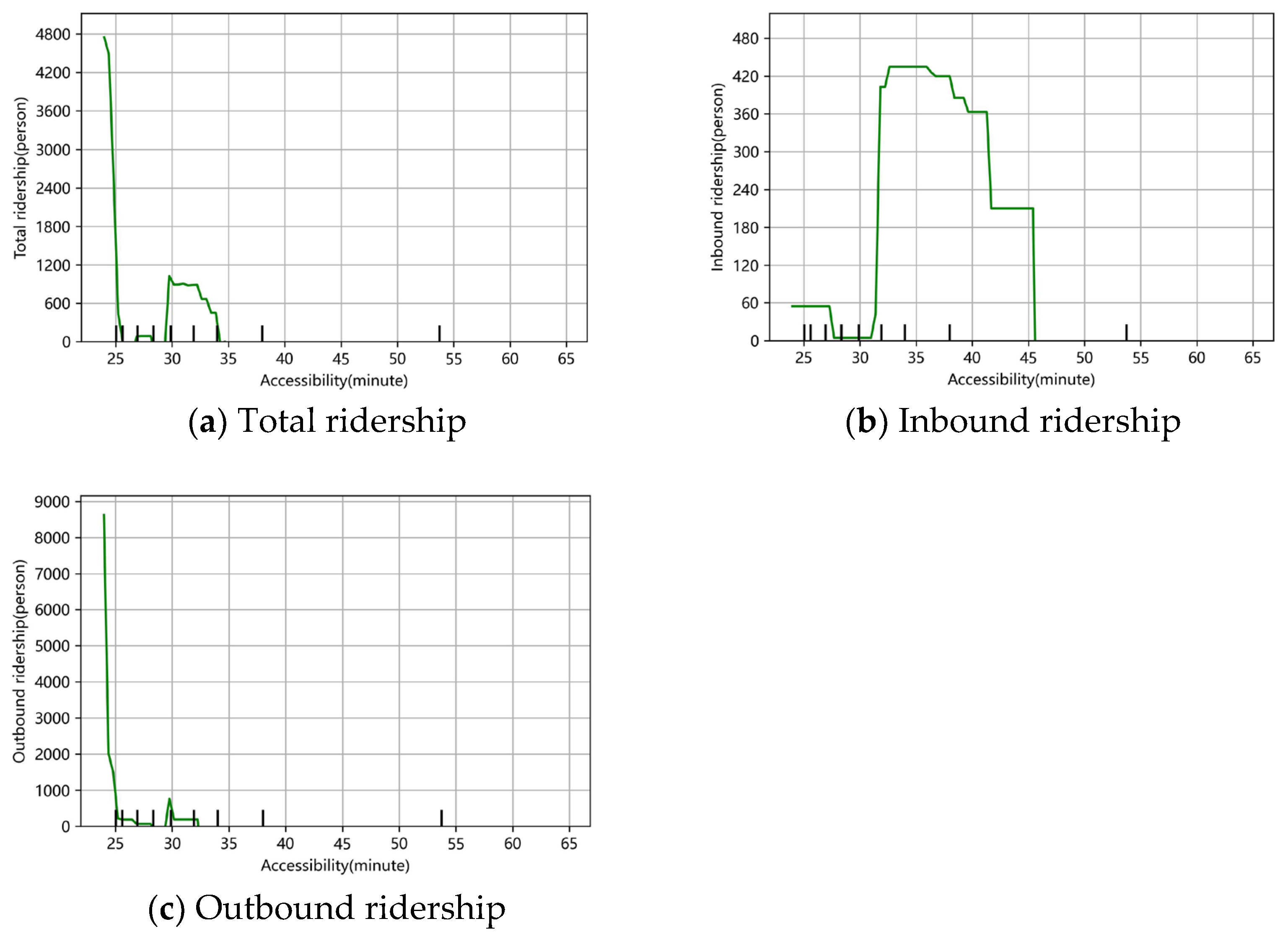
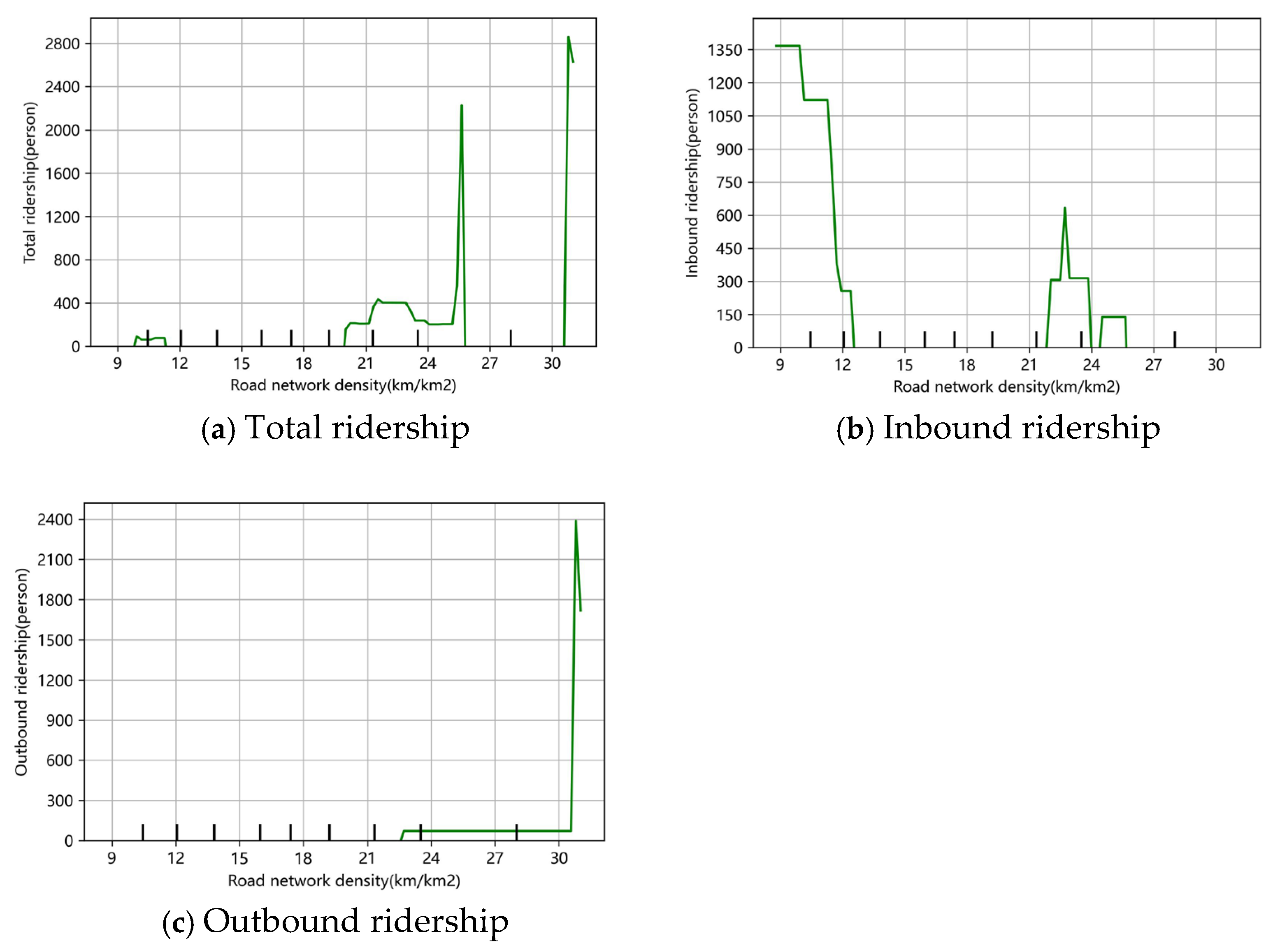
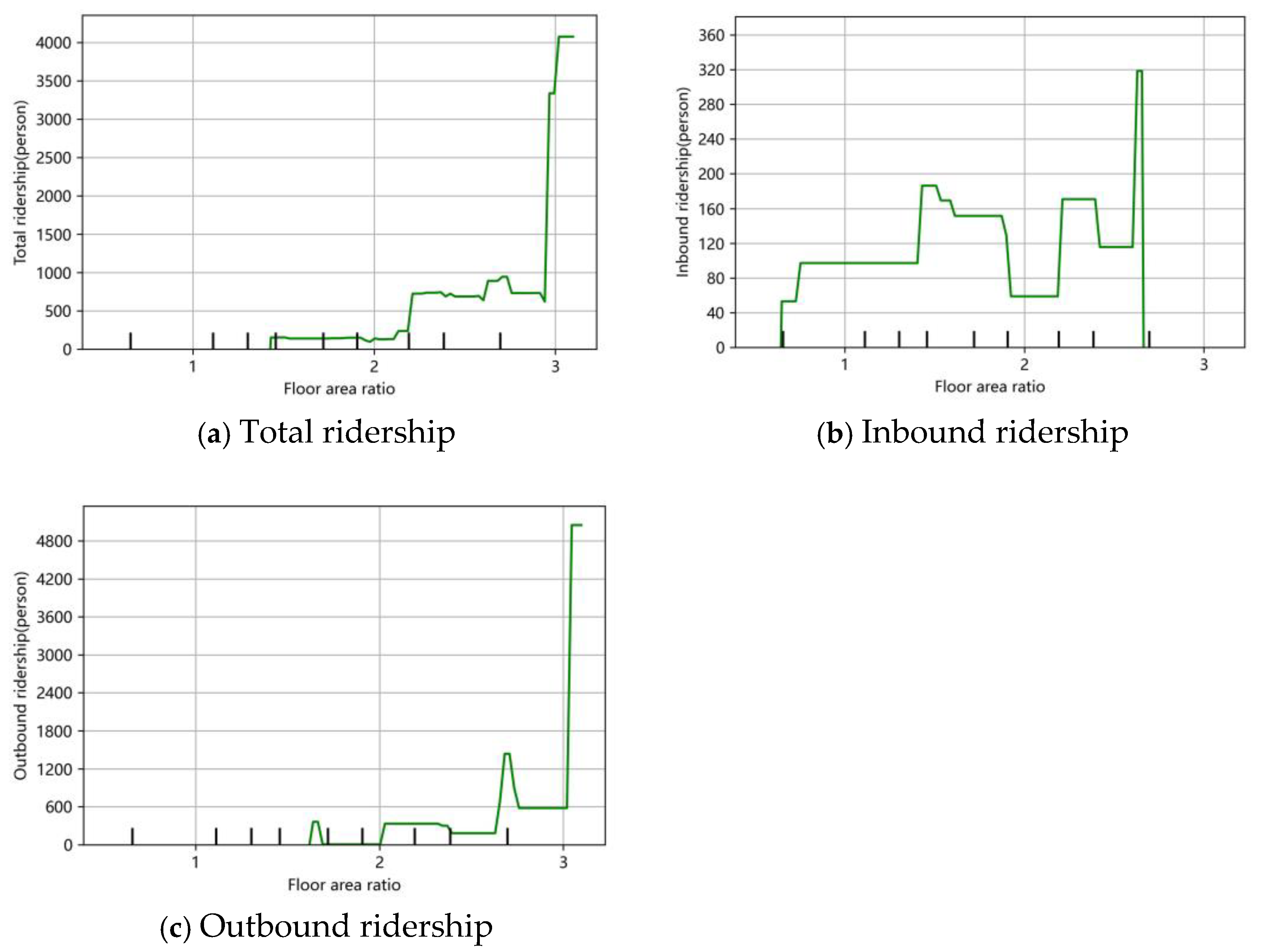
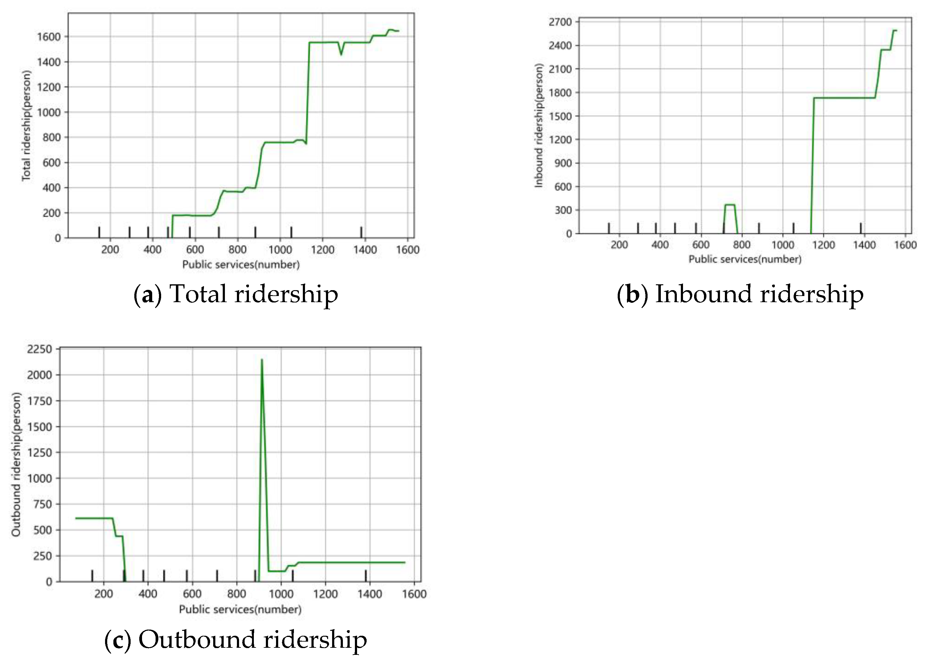
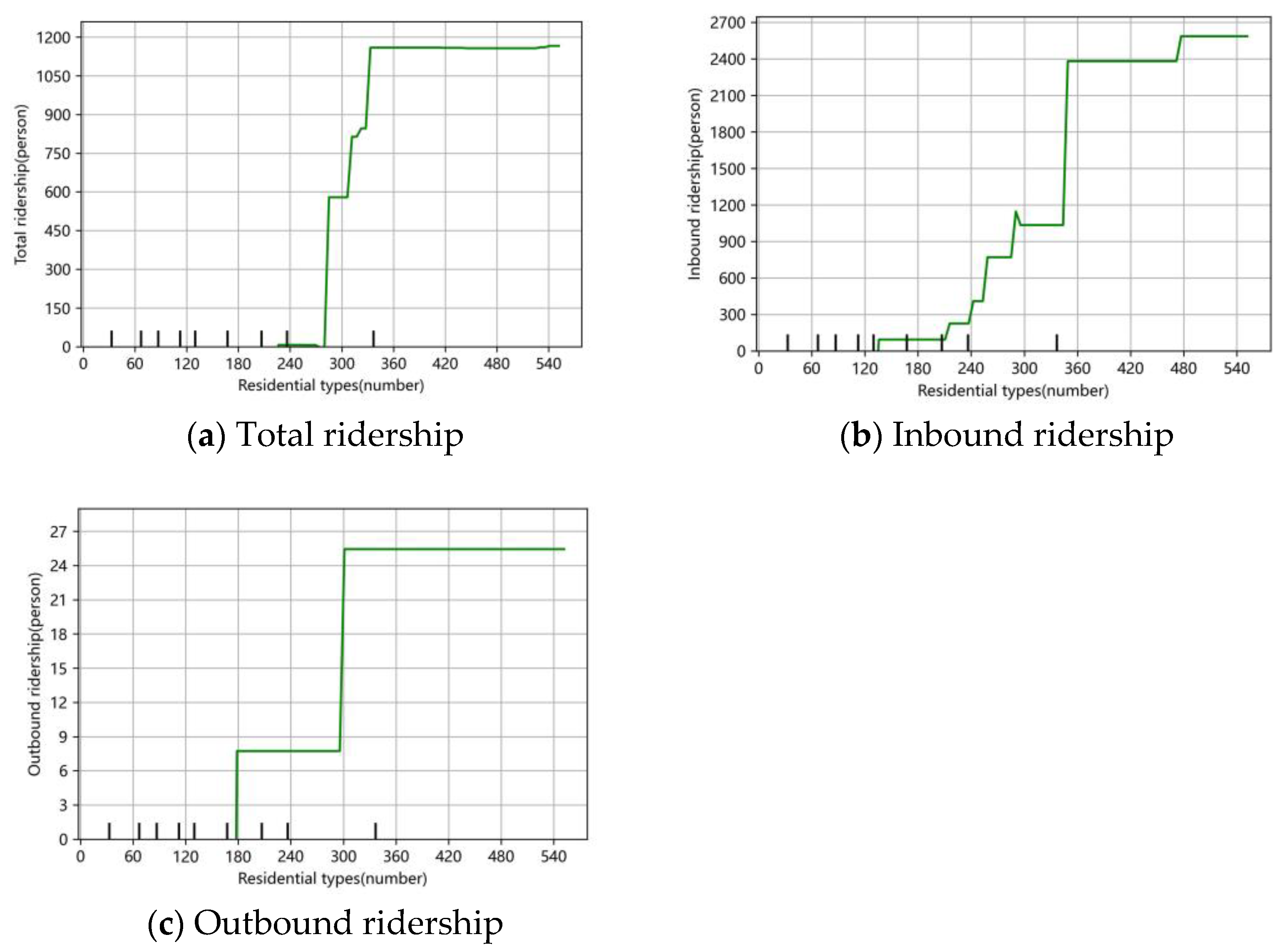


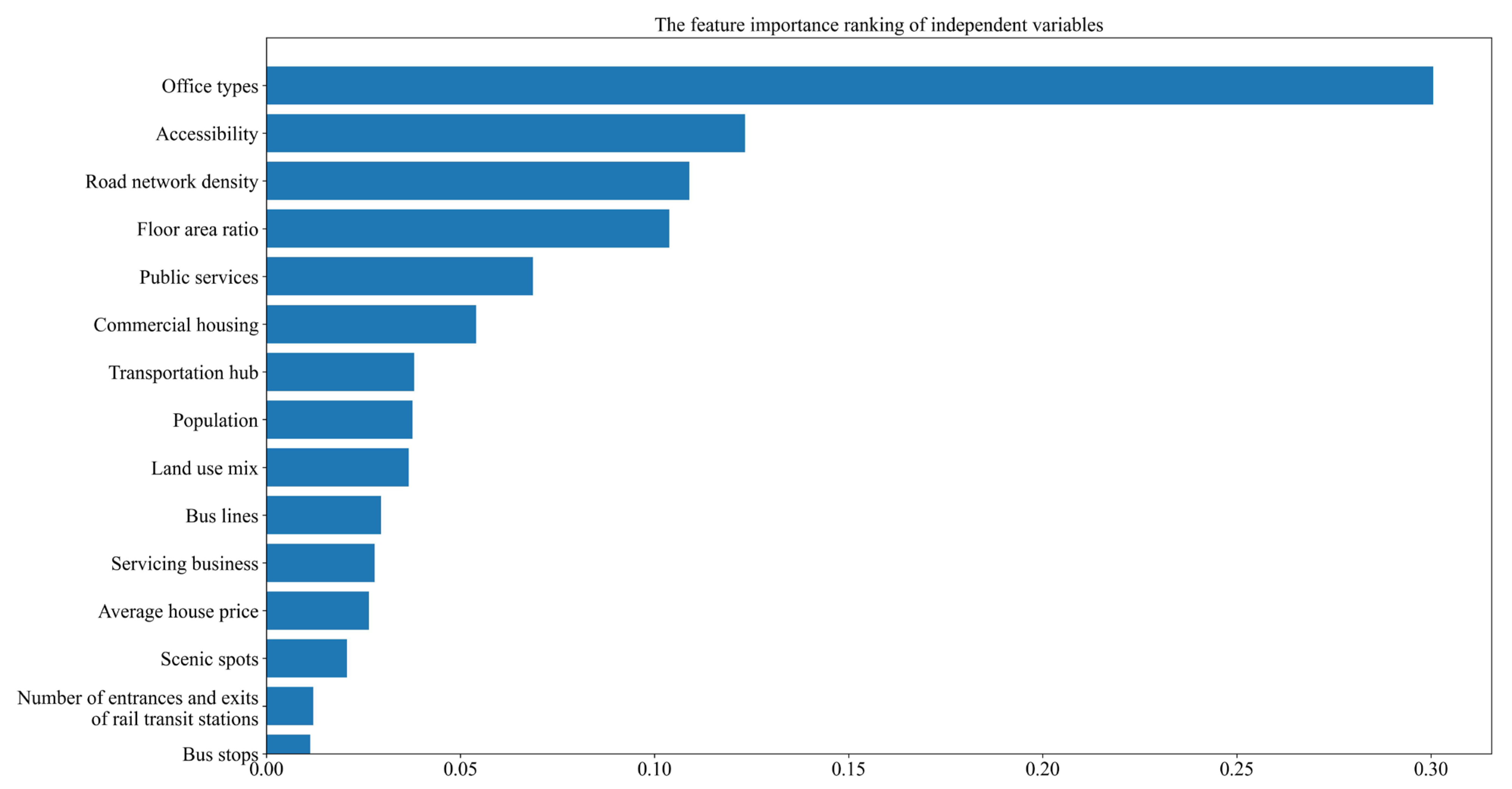

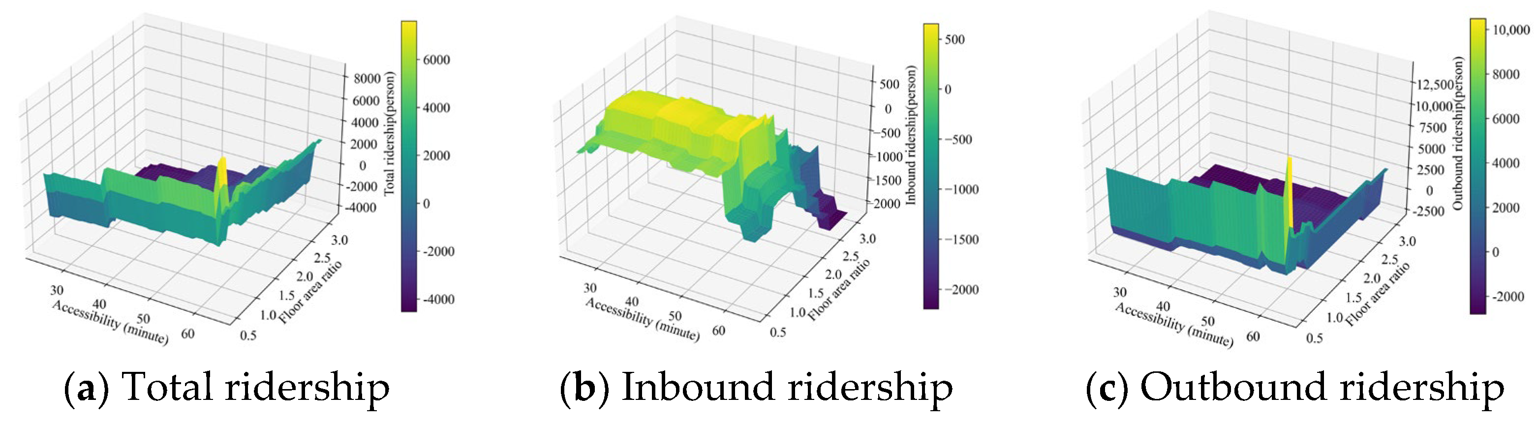
