Abstract
Accurate time series forecasting is crucial in fields such as business, finance, and meteorology. To achieve more precise predictions and effectively capture the potential cycles and stochastic characteristics at different scales in time series, this paper optimizes the network structure of the Autoformer model. Based on multi-scale convolutional operations, a multi-scale feature fusion network is proposed, combined with date–time encoding to build the MD–Autoformer time series forecasting model, which enhances the model’s ability to capture information at different scales. In forecasting tasks across four fields—apparel sales, meteorology, finance, and disease—the proposed method achieved the lowest RMSE and MAE. Additionally, ablation experiments demonstrated the effectiveness and reliability of the proposed method. Combined with the TPE Bayesian optimization algorithm, the prediction error was further reduced, providing a reference for future research on time series forecasting methods.
1. Introduction
1.1. Literature Review
For a long time, time series forecasting has been a key research focus in various fields, including business, industry, transportation, finance, and meteorology [1], to understand the underlying trends and patterns of data through data points [2]. Accurate time series forecasting helps enterprises seize market opportunities, prepare for potential challenges in advance, and effectively regulate resource allocation, thereby reducing costs and increasing efficiency [3]. In finance, time series prediction methods strongly support stock price forecasting [4,5] and macroeconomic indicator forecasting [6], offering references for investors’ decision-making [7]. Therefore, time series forecasting is not only an efficient data analysis technique but also an extremely valuable decision-support tool. It plays a vital role in various fields of modern society, and its importance goes without saying.
Currently, time series forecasting methods can generally be divided into two categories: statistical methods and machine learning methods [8,9,10]. Statistical methods are commonly used for forecasting tasks with lower-complexity time series data, such as ARIMA [11], SARIMA [12], and Grey Model (GM) [13], among others, which are quantitative forecasting methods. These statistical methods are usually simple and easy to implement, making them suitable for medium-and short-term predictions. For instance, in reference [14], the SFOR-ELM model based on data mining effectively predicted e-commerce sales data through grey relational analysis and optimization algorithms, thereby improving the efficiency of e-commerce management. Traditional machine learning methods, when combined with statistical approaches, can be applied to small-scale, rapid-forecasting tasks. For example, Zhou et al. [15] proposed a Bass model for rapid apparel demand forecasting based on the similarity of clothing and consumer preferences, combined with statistical principles, providing a reference for apparel sales forecasting.
However, the main bottlenecks of such research are manifested in two aspects: First, while traditional statistical methods perform reasonably well on low-complexity time series datasets, in practical time series forecasting tasks, the target sequences are often influenced by many exogenous factors such as seasonal trends. Traditional statistical-based methods struggle to achieve precise modeling [16]. Second, the above-mentioned methods have the insufficient capability to extract implicit features from data, making it difficult to uncover long-term cyclical patterns embedded in the data. They are also susceptible to short-term fluctuations and noise, which can lead to larger prediction errors and consequently affect corporate inventory management and sales.
With the development of machine learning, researchers have proposed hybrid models like GRU-Prophet [17], SARIMA-CNN-LSTM [18], and ARIMA-LSTM [19,20,21] to overcome the limitations of traditional statistical methods and improve time series forecasting accuracy. These models combine machine learning and statistical methods to capture time series information more comprehensively and have been widely applied in practice.
In deep learning research, the authors of [22] presented the Autoformer model based on the Transformer, innovatively developing the self-correlation attention mechanism for periodic feature extraction and adaptive frequency component selection in the frequency domain. Many scholars have improved and applied the Autoformer. The authors of [23] combined a genetic algorithm and an elite voting operator to create the GA-Autoformer model, which significantly enhanced pollution prediction accuracy in smart city management. Literature [24] built a hybrid ECA-CAE and Autoformer architecture, achieving high-precision life-span prediction for mechanical systems even with incomplete degradation data. These studies confirm the effectiveness of Autoformer-based time-series prediction methods, especially for long-period periodic data, where their superior performance is evident.
1.2. Research Hypotheses and Methodology
Autoformer, despite its good performance in many forecasting tasks, has three main limitations in time-series forecasting: imperfect embedding of temporal feature information; a single-scale convolution-based seasonal decomposition pattern with limited representation for complex multi-scale periodic patterns and difficulty in capturing dynamic trends; and model parameter configuration reliant on human expertise, restricting cross-domain applications.
To address Autoformer’s limitations and verify the hypotheses, this paper makes the following key contributions:
- A multi-scale feature fusion network suitable for time series is proposed. Based on convolutions at different scales, it can effectively extract multi-scale features of time series.
- Based on the above-mentioned feature fusion network, combined with date–time encoding [25], a time-series prediction method, MD–Autoformer, is proposed. Comparative experiments and ablation experiments are carried out with baseline models on real-world clothing sales datasets and time-series datasets from multiple fields, verifying the effectiveness of the method proposed in this paper.
- We optimized the MD–Autoformer’s hyperparameters using the TPE-based Bayesian algorithm, identifying the best parameters to enhance its prediction performance, making it more reliable and effective across diverse tasks.
The key research hypotheses explored in this study include:
Research Hypothesis 1 (RH1):
Introducing date–time encoding as a covariate can enhance the Autoformer model’s ability to perceive time information.
Research Hypothesis 2 (RH2):
Using a multi-scale feature fusion network can strengthen the model’s ability to perceive dynamic trends, reduce significant errors, and improve prediction accuracy.
Research Hypothesis 3 (RH3):
The hybrid MD–Autoformer model offers better performance than either adding a date–time coding module alone or a single multi-scale feature fusion module.
Research Hypothesis 4 (RH4):
Applying the Bayesian hyperparameter optimization algorithm can further enhance the model’s performance.
2. Materials and Methods
2.1. Data Source
This paper collected 3 million real sales records of a large mall in a certain country from the Kaggle data platform (https://www.kaggle.com/competitions/store-sales-time-series-forecasting/data, accessed on 16 February 2025), screened the apparel category, and aggregated it daily. The final dataset has 1683 apparel sales records from 2 January 2013 to 15 August 2017, measured daily. It was split into training, validation, and test sets in a 7:1:2 ratio, with 1176, 168, and 336 records, respectively.
During preprocessing, we first cleaned the data to remove missing values. Then, we standardized it to eliminate dimensional differences between features. Finally, we performed outlier detection to ensure data quality.
There is a close correlation between apparel sales and fashion trends. Therefore, to predict sales trends more accurately, this paper introduces Google Trends data as an auxiliary variable in the sales prediction task. The multi-dimensional features of data are crucial for improving the accuracy of time-series forecasting. As a supplementary information source, Google Trends data has been proven to be capable of effectively capturing socioeconomic dynamics and consumer behavior patterns. The authors of [26,27] jointly confirm the importance and effectiveness of Google Trends data in the apparel sales prediction task. By integrating multiple sales-related data sources, the model can comprehensively understand market dynamics, enabling more accurate sales predictions in the highly competitive fashion market.
The economy of the region where the dataset is sourced is significantly dependent on the export of the oil industry. Therefore, fluctuations in international oil prices and the US dollar index have a significant impact on the country’s macro-economy and consumption patterns. In this paper, we further expand the scope of data collection to include Google Trends data for keywords related to apparel categories in this region, aiming to uncover the potential correlations between consumer interests and economic variables. The features included in the dataset and their specific meanings are shown in Table 1.

Table 1.
Feature descriptions.
In feature engineering, we thoroughly analyzed the data to select features that best reflect apparel sales trends and related factors. We created multiple features, including historical sales data, the Google Trends index, oil prices, and the US Dollar Index, which are described in Table 1. Figure 1 shows the correlations between different variables in the final apparel sales dataset we built. To ensure the stationarity of the time series data, we conducted stationarity tests on all datasets. Specifically, we used the ADF (Augmented Dickey–Fuller) test to determine if the time series has a unit root and thus assess its stationarity. For non-stationary series, we applied differencing until the series met the stationarity requirements as indicated by the ADF test. Additionally, considering the common presence of seasonality in time series data, we also performed seasonal decomposition to further enhance the model’s forecasting performance.
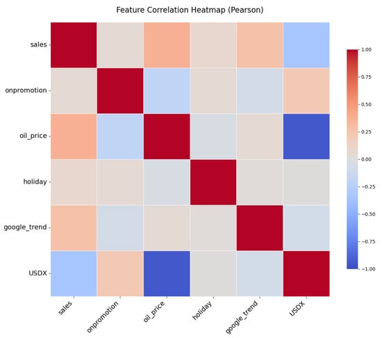
Figure 1.
Correlation matrix of the considered variables.
2.2. Autoformer Network Structure
Given the remarkable success of the Autoformer model in time series forecasting tasks, this paper adopts it as the foundational algorithm for our study. The Autoformer model employs an encoder–decoder architecture that integrates an autocorrelation network, a seasonal decomposition network, and a feed-forward neural network. The seasonal feature information generated by the encoder serves as the input for the decoder’s autocorrelation network. The encoder is dedicated to seasonal modeling, extracting periodic features through the use of autocorrelation and seasonal decomposition networks, while the feed-forward network further delves into extracting more profound features. The initial input to the decoder comprises both seasonal and trend components, with the trend being refined incrementally through the decomposition process, utilizing the crossover information yielded by the encoder. The detailed mathematical formulations for the seasonal decomposition network are presented in Equations (1) and (2). In Equation (1), denotes the original input time series. The term Padding refers to a bilateral padding operation, which is implemented to maintain the sequence length consistent with the required input length. The trend component is derived by employing an average pooling operation, denoted as AvgPool. In Equation (2), the original time series input is adjusted by subtracting the trend component , which was previously derived in Equation (1). This subtraction process isolates the seasonal component, denoted as , from the original data.
The implementation of the autocorrelation mechanism is facilitated through the Fast Fourier Transform (FFT), which enables the efficient computation of the sequence’s autocorrelation in the frequency domain. The autocorrelation coefficient is then derived by the formulation presented in Equation (3). In Equation (3), signifies the autocorrelation coefficient, indicates the total length of the observed time series, represents the value of the time series at time point , and denotes the time lag interval. Consequently, Equation (3) serves to measure the degree of similarity between the time series before and after the lag is applied. Time series that exhibit potential cyclical patterns are characterized by high similarity values. The autocorrelation coefficient can be computed by the Wiener–Khinchin theorem [28], utilizing the Fast Fourier Transform as detailed in Equations (4) and (5).
In Equation (4), represents the Fourier transform of the autocorrelation, where signifies the Fast Fourier Transform (FFT) and denotes the conjugate operation. Moving to Equation (5), corresponds to the autocorrelation value of the time series at a lag of , and represents the inverse Fourier transform. By applying the inverse Fourier transform to Equation (4), we can convert the frequency–domain autocorrelation to the time–domain autocorrelation coefficient.
The autocorrelation mechanism analyzes the autocorrelation under different time lags, identifies the periodic patterns of the sequence, and selects representative lags. These time lags are used to align similar subsequences and global information is extracted through weighted aggregation. This method reduces the computational load and improves the efficiency of information utilization through sequence aggregation. The time-series prediction method based on the autocorrelation mechanism can focus on the seasonal components in the time series, effectively enhancing the model’s ability to extract data patterns and trends.
2.3. Proposed Method
2.3.1. Multi-Scale Feature Fusion Network
Time series data exhibits multi-scale characteristics encompassing long-term trends, short-term fluctuations, periodic patterns, and transient anomalies. Traditional single-scale convolutional operations struggle to capture these diverse temporal dependencies simultaneously. To address this limitation, we propose a multi-scale feature fusion network that systematically integrates hierarchical temporal features through parallel convolutional branches. As illustrated in Figure 2, the architecture comprises two principal components:
- The 1 × 1 convolutional branch specializes in inter-channel interactions and cross-scale feature recalibration. Through adaptive average pooling along the temporal dimension, this branch extracts compressed global contextual information while preserving channel interdependencies.
- The 3 × 3 convolutional branch extends the receptive field along the temporal axis, enabling the model to capture both localized temporal patterns and extended dependencies. This configuration facilitates the identification of seasonal patterns and macro-trends while discriminating between high-frequency noise and low-frequency trends through differentiated frequency responses of convolutional kernels [29].
The feature fusion mechanism employs grouped processing of feature maps with subsequent pooling, convolution, and normalization operations. This architecture maintains channel interdependencies while enhancing multi-scale feature extraction capabilities, which proves essential for modeling complex temporal dynamics where cross-scale information interactions occur.
The multi-scale feature fusion network effectively enhances the model’s ability to extract multi-scale features from time series data by integrating features from different convolutional kernels. It provides more comprehensive and accurate feature representations for time series forecasting tasks. This allows the model to better learn both short-term and long-term dependencies in time series data and extract temporal features at different scales.
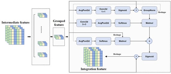
Figure 2.
The structure of time series-based multi-scale feature fusion networks, the symbol * denotes element-wise multiplication between tensors of the same shape.
2.3.2. Date–Time Encoding
In time-series prediction tasks, accurately capturing and modeling the inherent periodicity and dynamic trends of time-series data is one of the core challenges. For most time-series data, there are often certain operating rules and periodicity. Therefore, making full use of the periodic time information in the data can provide strong support for trend prediction. In this paper, the date–time encoding method is adopted. The date and month variables in the time variables are mapped within one period of the sine and cosine functions to become new static covariates. Based on the continuity and periodicity of trigonometric functions, the new encoding ensures uniqueness while maintaining continuity and periodicity, aiming to improve the model’s sensitivity to temporal dynamics and prediction accuracy. From the perspective of model input architecture, conventional Transformer models typically adopt element-wise addition between encoded features and embedding vectors, while we introduce encoded multi-dimensional temporal features as independent covariate channels. This feature fusion strategy allows temporal information to participate in feature interactions as explicit covariates, effectively enhancing the model’s ability to characterize periodic temporal patterns.
The specific calculation formula for the date encoding values is shown in Equations (6)–(9), with the encoding range being [−1, 1], where m represents the month and d represents the day.
2.3.3. Prediction Model
Integrating the sub-methods proposed above, this paper presents a time-series prediction model, named MD–Autoformer, which is based on Autoformer. This model incorporates multi-scale feature fusion and date–time encoding techniques, and its network structure is shown in Figure 3. The input data of the model includes multiple features closely related to apparel sales. The input of the encoder is denoted as , where represents the length of the sequence and d represents the dimension of the data. The input of the decoder mainly consists of two parts: the seasonal component input and the trend component input . Both parts are provided by the encoder with extracted information of length , where is a placeholder used to fill in the initial values of the predicted sequence. The mathematical expressions of the model’s input are shown in Equations (10)–(12). and represent the zero-padding placeholder and the mean value of , respectively.
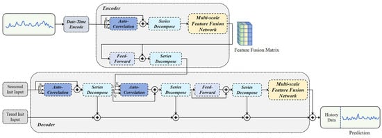
Figure 3.
The network architecture of MD–Autoformer.
The multi-scale feature fusion matrix processed by the encoder is combined with the seasonally initialized input and the trend-initialized input. It is then processed again through the automatic correlation mechanism and the sequence decomposition module. Finally, the seasonal decomposition module and the multi-scale feature fusion network further extract deep features, enhancing the model’s nonlinear expression capability and generating the final prediction results. This process not only takes into account the seasonality and trend components of the time series, but also captures the subtle features in the sequence through the multi-scale feature fusion network, thereby improving the model’s ability to explain the periodicity and random disturbances of the time series.
The MD–Autoformer addresses stationarity and seasonality through the following mechanisms: First, the seasonal decomposition module in the Autoformer framework separates time series into seasonal and trend components using moving average operations to isolate periodic patterns. Second, the multi-scale feature fusion network enhances multi-periodicity modeling through parallel convolutional branches with varying receptive fields. For stationarity, two practical measures are implemented: (1) input normalization stabilizes statistical properties across features, and (2) in data preprocessing, we conduct the Augmented Dickey–Fuller (ADF) test for stationarity. Non-stationary series undergo first-order differencing until passing the ADF test. This combined strategy ensures robust handling of both stationary and non-stationary components in time series.
3. Results
3.1. Experimental Parameters and Evaluation Metrics
3.1.1. Experimental Parameters
The experimental setup was equipped with a 13th Gen Intel(R) Core(TM) i7-13700KF processor (Intel, Santa Clara, CA, USA), operating at a speed of 3.40 GHz, complemented by an NVIDIA GeForce RTX 4070 Ti SUPER GPU (Nvidia, Santa Clara, CA, USA) for accelerated graphics processing. The system ran on Windows 11 and was configured with a deep learning development environment based on CUDA 11.8.
In the course of the experiments, the batch size for model training was configured at 32. The optimization algorithm employed was Adam, with the early-stopping criterion set to a patience of 3 epochs. The training was conducted utilizing the L2 loss function, with the learning rate set to . Our model was trained with specific architectural parameters: a model dimensionality of 512, a hidden layer dimensionality of 2048, 8 heads in the multi-head attention mechanism, 2 layers in the encoder, 1 layer in the decoder, and the GELU activation function was used throughout the model.
3.1.2. Evaluation Metrics
In this paper, to assess the performance of the time series forecasting model, we utilize Root Mean Squared Error (RMSE) and Mean Absolute Error (MAE) as our evaluation metrics. RMSE calculates the square root of the average of the squared differences between predicted and actual values, and it is measured in the same units as the original data, thereby directly reflecting the standard deviation of the discrepancies between predictions and actuals. On the other hand, MAE evaluates the average of the absolute differences between predicted and actual values, giving equal weight to all error magnitudes and offering an unbiased estimate of the prediction errors. A comprehensive analysis using both RMSE and MAE metrics allows for a more objective and precise evaluation of the model’s predictive accuracy. The formulas corresponding to these evaluation metrics are presented in Equations (13) and (14).
In which and represent the true value and the predicted value of the target sequence, respectively, and denotes the number of samples.
3.2. Clothing Sales Forecasting: Case Study
To evaluate the effectiveness of the proposed method on the apparel sales forecasting task, we conducted a comparative experiment between the proposed method and Autoformer, Informer [30], Reformer [31], and DLinear [32] on a real apparel sales forecasting task, and the experimental results are shown in Table 2.
Table 2.
Comparative experimental results for different prediction step sizes on Apparel Sales.
The experiments were conducted independently multiple times, and the average values were taken to minimize the potential interference of random factors on the model evaluation results. The experimental results show that our proposed method outperforms other classical methods in most cases. Specifically, at 24-step forecasting, our method achieves a RMSE of 2.165 and an MAE of 0.761, which are significantly lower than the other models compared, and have higher forecasting accuracy. From the trend analysis of errors, compared to Autoformer, when the prediction step size is 24, MD–Autoformer achieved a 24.47% reduction in RMSE and a 39.33% reduction in MAE; when the prediction step size increased to 60, the RMSE decreased by 22.36%, and the MAE decreased by 24.93%. DLinear also performs well. In the experiment with a prediction length of 60, DLinear’s RMSE is 2.852 and MAE is 1.146, which is more accurate than Autoformer’s prediction. This indicates that MD–Autoformer has a significant advantage in short-term apparel sales forecasting, particularly excelling in reducing the mean absolute error.
Due to the lack of ability to extract time series information for different scales with seasonal trend prediction, the experimental errors demonstrated by Informer and Reformer gradually expand with increasing prediction steps, while our method has a lower growth rate of errors in 36, 48, and 60-step prediction, which further verifies that multi-scale feature fusion networks with date–time coding can effectively extract the hidden information of time series of different lengths, which overall improves the prediction performance for long-time apparel sales tasks.
In the Apparel Sales forecasting experiment, we focus not only on the prediction accuracy of the model but also on its stability and reliability. For this purpose, we have conducted a standard deviation analysis of the experimental results of each model.
As shown in Table 3, the MD–Autoformer model has relatively small standard deviations in RMSE and MAE across different prediction steps. This indicates that the model performs consistently in multiple experiments with little fluctuation in prediction errors. In contrast, other models like Informer and Reformer have larger standard deviations, meaning their prediction results vary more significantly across different experiments, making them less stable.
Table 3.
Standard deviation of each model in apparel sales forecasting experiment.
In summary, the MD–Autoformer model not only excels in prediction accuracy but also demonstrates a clear advantage in stability. This makes the model more reliable for practical applications, providing stable decision-making support for tasks like apparel sales forecasting.
Figure 4 provides a detailed comparison of our proposed forecasting method with other models in the task of apparel sales forecasting. Upon comparative analysis, it is evident that our method demonstrates a significant advantage in overall predictive accuracy. Particularly when dealing with long-term forecasting tasks, our approach more accurately approximates the actual apparel sales data, indicating that our model possesses a stronger capability in capturing the long-term dependencies and seasonal patterns of time series data.
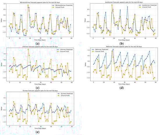
Figure 4.
Prediction results of different models when the prediction time step is 60. (a) MD–Autoformer; (b) Autoformer; (c) Informer; (d) Reformer; (e) DLinear.
The experimental results highlight the better performance of our method in mitigating the fluctuations that may occur in long-term forecasting and the resultant extreme prediction errors. This is especially crucial for datasets with pronounced seasonality and trends, such as those in apparel sales forecasting, where higher demands are placed on the precision and robustness of the forecasting models. The experimental outcomes further substantiate the effectiveness of our method in practical applications, particularly in commercial environments where accurate predictions are essential for guiding inventory management and the formulation of sales strategies.
3.3. Method Validation on Diverse Data
To fully evaluate the proposed method’s effectiveness, this paper conducts comparative experiments in three fields: disease, finance, and meteorology, where time-series forecasting methods are widely used. In the experiment, the datasets are split into training, validation, and test sets in a 7:1:2 ratio. Additionally, the RMSE and MAE values reported in this section are averages obtained from multiple repeated experiments.
3.3.1. Prediction Experiments in the Disease Field
In real life, the spread of infectious diseases and apparel sales are both closely related to seasonal changes. Their time-series data features are affected by seasonal and trending factors, showing certain patterns. Therefore, we give priority to the disease-related dataset for testing. In the disease field, we chose the Illness (ILI) dataset for time-series prediction. The ILI dataset contains weekly records of influenza-like illness (ILI) patients from the US Centers for Disease Control and Prevention during 2002–2021, reflecting the proportion of ILI patients among all patients.
On the ILI dataset, the MD–Autoformer model shows superior predictive performance. As shown in Table 4, MD–Autoformer has lower RMSE and MAE values than other models at different prediction steps. For instance, at 24-step prediction, MD–Autoformer’s RMSE is 1.385 and the MAE is 0.834, compared to 1.866, 2.401, 2.098, and 1.489 for RMSE, and 1.287, 1.677, 1.382, and 1.084 for the MAE of Autoformer, Informer, Reformer, and DLinear, respectively. This indicates that the MD–Autoformer can capture the periodicity and trending characteristics of disease data more accurately.
Table 4.
Experimental results of different models on ILI dataset.
Moreover, the MD–Autoformer has smaller standard deviations at different prediction steps, showing higher stability. For example, at 60-step prediction, its RMSE standard deviation is ±0.039, and the MAE standard deviation is ±0.015. A low standard deviation indicates that MD–Autoformer maintains a stable level of precision in repeated experiments.
As shown in Figure 5, MD–Autoformer, Autoformer, and DLinear all effectively capture the upward and downward trends in disease data, with their changing trends being consistent with the true values at multiple peaks or troughs. Although DLinear has slightly higher RMSE and MAE than MD–Autoformer, its ability to capture sequence trends is commendable.
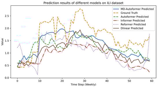
Figure 5.
Experimental results of different models on ILI dataset.
In summary, MD–Autoformer outperforms other models on the ILI dataset, particularly in capturing long-term dependencies and seasonal patterns. This is mainly due to its multi-scale feature fusion network and date–time encoding module, which effectively extracts key information from time-series data to improve prediction accuracy and stability.
3.3.2. Prediction Experiments in the Financial Field
Finance is closely related to time series prediction. Accurate time series prediction can inform investment decisions in stocks [33,34], gold [35], and currencies [36], and enable more in-depth predictions when combined with financial indices [37,38], with broad applications.
Exchange [39] is a widely used dataset for time series methodology evaluation, containing daily exchange rates for eight countries from 1990 to 2016. We conducted a comparison experiment with four different prediction lengths on the Exchange dataset. During the experiments, the lookback window lengths were set to 96 for Transformer-based models and 336 for DLinear.
The results are presented in Table 5 and Figure 6. Based on error metrics, DLinear achieved the lowest RMSE and MAE values. Although MD–Autoformer ranked second to DLinear, it demonstrated higher prediction accuracy than Autoformer. As shown in Figure 6, while DLinear exhibited higher volatility, it delivered more precise predictions at most time points. MD–Autoformer’s fluctuations closely followed actual trend variations and aligned better with true values at peaks and troughs. In contrast, Autoformer struggled to capture subtle trend changes and generated more outlier errors. Both Reformer and Informer underperformed significantly.
Table 5.
Experimental results of different models on Exchange.
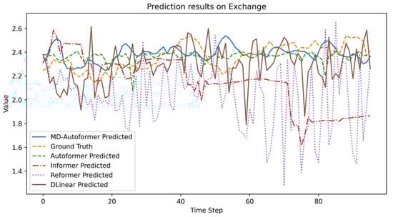
Figure 6.
Experimental results of different models on the Exchange.
To further validate the capability of MD–Autoformer in high-frequency financial time series forecasting tasks, we collected data from QQQ, an ETF managed by Invesco Ltd. (Atlanta, GA, USA) that tracks the NASDAQ-100 Index. The dataset spans from 10 March 1999 to 10 November 2017 and includes daily metrics such as open, close, high, and low prices, and trading volume. We conducted comparative experiments targeting the prediction of closing prices over a 60-day horizon.
During the experiments, the lookback window lengths of baseline models were allowed to vary. This design accounts for the observation that Transformer-based models tend to overfit with extended lookback windows, while DLinear exhibits underfitting tendencies. Consequently, the lookback window length was set to 96 for Transformer-based models and 336 for DLinear. Each model underwent 30 trial runs, and the mean values and variances of RMSE and MAE were calculated. Detailed experimental results are presented in Table 6 and Figure 7.
Table 6.
Performance comparison of different models in 60-day closing price forecasting on QQQ.
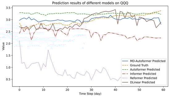
Figure 7.
The prediction results of QQQ-ETF closing price by different models.
As shown in Table 6, compared with Autoformer, MD–Autoformer reduces RMSE by 10.41% and MAE by 6.29%, indicating a marked rise in forecasting accuracy. DLinear and Autoformer also show low RMSE and MAE, meaning their prediction values are close to the true values. Figure 7 reveals that MD–Autoformer and DLinear have trends closer to the true values. Despite its high forecasting efficiency, DLinear’s simple network structure causes large prediction fluctuations. Informer detects market downturns but has high errors. Autoformer suffers from over-smoothing and cannot reflect market trends well.
Although the MD–Autoformer can capture the general trend of ETFs, its sensitivity and accuracy are insufficient for real-market transactions in high-frequency trading scenarios. Thus, improvements are required in future work.
3.3.3. Prediction Experiments in the Meteorological Field
In the weather forecasting experiment, we used the Weather dataset, a common dataset in time series prediction, for comparative experiments. This dataset, sourced from the meteorological field, includes 21 weather-related indicators. Each record covers a 10-min time span, and the entire dataset spans one year.
The experimental results of different models on the Weather dataset are shown in Table 7 and Figure 8. Since the Weather dataset has 21 correlated variables, it contains a large volume of information and poses higher prediction difficulty. In the experiment with a prediction step of 192, none of the models mentioned in this paper performed ideally. From the evaluation metrics, MD–Autoformer and DLinear performed well, with their predicted values roughly following the trend of the ground truth. DLinear has slightly lower RMSE and MAE than MD–Autoformer, mainly due to its higher prediction stability. Although the predicted values of MD–Autoformer have some fluctuations, they still fit the trend of the ground truth well.
Table 7.
Experimental results of different models on Weather dataset.
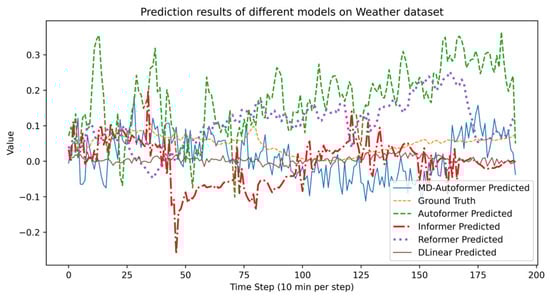
Figure 8.
Experimental results of different models on the Weather.
As shown by the experimental results in multiple fields, MD–Autoformer can capture time information at different scales more precisely, especially on datasets with significant periodicity and trends. Compared to Autoformer, it enhances prediction stability and accuracy while maintaining the ability to capture sequence trends.
3.4. Model Performance Evaluation
3.4.1. Convergence
Figure 9 presents the training and validation loss curves of MD–Autoformer across four datasets. The model shows good convergence on all datasets, with both training and validation losses decreasing during training and then stabilizing, indicating effective feature learning and fitting on datasets.
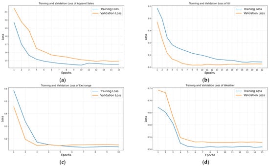
Figure 9.
Loss curves of MD–Autoformer on various datasets. (a) Apparel Sales; (b) ILI; (c) Exchange; (d) Weather.
For MD–Autoformer, when trained on small datasets (e.g., Apparel Sales and ILI), it needs more training epochs to converge. This is because it is harder to learn the data’s underlying patterns and the model usually has smaller hidden dimensions. In contrast, when trained on larger datasets (e.g., Exchange and Weather), the abundance of data allows the model to quickly learn sequence patterns. Meanwhile, higher hidden dimensions help faster convergence, so fewer training epochs are needed.
During model training, to prevent overfitting, we used several effective strategies. First, we applied Dropout technology, randomly deactivating some neurons in fully connected layers. This enhanced the model’s generalization ability. Second, we adopted early stopping, closely monitoring the validation set loss. Training was terminated early when the loss stopped decreasing, preventing overfitting to training data. Last, we properly adjusted the hidden layer dimensions during training to avoid overfitting caused by too many parameters. Using these methods together ensured the model could learn useful data information fully while effectively avoiding overfitting. This resulted in better generalization and prediction accuracy in practical applications.
3.4.2. Computational Time Analysis
Table 8 compares the average epoch time cost of different models across four datasets. MD–Autoformer shows a time cost increase of approximately 4.8% in Apparel Sales, 3.9% in ILI, 17.2% in Exchange, and 5.6% in Weather compared to Autoformer. This indicates that the MD–Autoformer achieves higher accuracy with only a slight increase in computational time, which is acceptable. DLinear, with its linear network structure, demonstrates high computational efficiency and good accuracy, such as taking only 2.882 s on the weather dataset. In conclusion, the trade-off between accuracy improvement and time cost increase in MD–Autoformer is reasonable, while DLinear maintains good accuracy with high efficiency, making them suitable for different scenarios.
Table 8.
Comparison of average epoch time cost for Maximum Step Prediction Tasks on different datasets.
3.4.3. Parameter Sensitivity
To evaluate the impact of different hyper-parameters on the MD–Autoformer’s performance, we focused on the number of channels divided in the MSFFN (denoted as ) and conducted experiments across four datasets. The experimental results are shown in Table 9.
Table 9.
MD–Autoformer performance under different choices of hyper-parameter in the MSFFN. We adopt the forecasting setting as input-36-predict-48 for the ILI and Apparel Sales datasets, and input-96-predict-336 for the other datasets.
For small-scale datasets like Apparel Sales and ILI, increasing the number of channel divisions in the MSFFN allows the model to learn more inter-channel interaction features, thereby improving performance. However, for large-scale datasets such as Weather and Exchange, excessive channel division may lead to the loss of interaction information between original hidden dimensions, resulting in decreased model performance.
In summary, the optimal number of channel divisions in the MSFFN varies by dataset scale. Small datasets benefit from more channel divisions to capture inter-channel interactions, while large datasets require a balance to avoid losing critical interaction information.
3.5. Statistical Significance Analysis
To verify the statistical significance of the model improvements, this study selected experimental results with the longest prediction horizon from each dataset: Apparel Sales (60 steps), ILI (60 steps), Exchange (720 steps), and Weather (720 steps). Paired t-tests were performed between MD–Autoformer and Autoformer to demonstrate the statistical significance of our improvements. The experimental data consisted of the MAE metric from 30 independent runs in each scenario.
As shown in Table 10, MD–Autoformer achieves significantly lower MAE than Autoformer across all datasets. For the Apparel Sales and ILI datasets, the t-statistics are 57.63 and 47.91, respectively, with p-values less than the critical value α = 0.01, indicating extremely significant differences. Similarly, for the Exchange and Weather datasets, the t-statistics are 20.70 and 20.95, respectively, also with p-values less than α = 0.01. These results demonstrate that the improvements of MD–Autoformer over Autoformer are not only statistically significant but also highly reliable. The mean differences in MAE further confirm that MD–Autoformer provides more accurate forecasts than Autoformer.
Table 10.
Statistical significance analysis of MD–Autoformer vs. Autoformer.
3.6. Ablation Study
The ablation experiments are mainly aimed at evaluating the contributions of the multi-scale feature fusion network and the date–time encoding module to the overall performance of the MD–Autoformer model. The results of the ablation experiments are shown in Table 11.
Table 11.
Results of ablation experiments.
According to the results of the ablation experiments, in three datasets with different lengths and from different fields, MD–Autoformer, which simultaneously incorporates the multi-scale feature fusion network and the date-encoding module, outperforms other models in terms of the Root Mean Square Error (RMSE) and Mean Absolute Error (MAE) metrics, achieving the optimal performance level of the model. As the prediction step size continuously increases, the impact of the multi-scale feature fusion module on RMSE and MAE becomes more and more significant. This is particularly evident in the Exchange dataset. When the prediction step size is 720, compared with Autoformer, the MSE decreases by approximately 9.73% and the MAE decreases by approximately 11.26%. The effect is more obvious compared to short-term prediction tasks.
On the one hand, the introduction of date–time encoding enhances the model’s ability to capture time-related periodic information in the sequence. On the other hand, the multi-scale feature fusion module can mitigate the prediction errors caused by short-term fluctuations in the original sequence. It also reduces the interference of random components in the original data and decreases extreme errors, thus making the trend of the prediction results closer to the actual values.
3.7. Bayesian Hyperparametric Optimization Experiments
In hyperparameter optimization, genetic algorithms have the advantage of global search in high-dimensional parameter spaces and avoiding local optima. However, they require generating and evaluating many individuals each generation, consuming significant computing resources and increasing optimization time. In time-series forecasting research, many scholars have enhanced forecasting accuracy using Bayesian hyperparameter optimization. For example, Zulfiqar et al. [40] improved BNN-based electricity load forecasting accuracy with this algorithm. Jiang et al. [41] used it to boost the accuracy of the Attention-LSTM method for room temperature forecasting. Du et al. [42] enhanced the accuracy of the BODE in multiple fields through Bayesian optimization. These studies show the algorithm’s good performance in time-series forecasting.
After evaluation, we chose the TPE-based Bayesian optimization algorithm. It uses computing resources more efficiently, quickly exploring the hyperparameter space with less consumption. Especially with large hyperparameter spaces, TPE converges to good solutions quickly, greatly improving optimization efficiency. Bayesian optimization algorithm (BOA) is a model-based method that builds conditional probability models of validation performance via surrogate functions [43]. Its core includes five elements: hyperparameter space, objective function, acquisition function, evaluation history, and surrogate function. The TPE-based method avoids re-evaluating poor hyperparameters by tracking historical assessments, unlike grid or random search.
The core innovation of the TPE method is the use of non-parametric density estimation technology, whose mathematical expression is shown in Formula (15). Here, represents the hyperparameters to tune, is the hyperparameter space, and are kernel density estimates (KED) based on historical good and ordinary samples, and is the observed data from the search process. The algorithm splits historical data into a good subset and a bad subset , building separate KED models. This dual-density approach better guides the exploration and exploitation of the hyperparameter space.
In this paper, to fully exploit MD–Autoformer’s potential in time series forecasting, we conduct experiments using the TPE-based Bayesian hyperparameter optimization algorithm, targeting MSE minimization. Algorithm 1 outlines the simplified TPE-based Bayesian optimization algorithm (BOA).
| Algorithm 1: TPE-based BOA for MD–Autoformer turning |
| Require: Objective function , hyperparameter space , maximum number of trials Ensure: Optimal , Minimal loss 1: Initialize observations 2: for to do 3: Partition into 4: Build density models: , 5: Select hyperparameters: 6: Evaluate hyperparameters: 7: Update observed data: 8: end for 9: return and ; |
Table 12 lists the key optimization parameters and their semantic interpretations for this study. The Dropout parameter controls the ratio of randomly dropped neurons during training to prevent overfitting. The Learning rate determines the step size for parameter updates. The train epoch indicates the number of training iterations. The MSFFN factor is the scaling coefficient for channel grouping in the multi-scale feature fusion network. During experiments, models are trained and evaluated using hyperparameter combinations generated by the BOA, which dynamically adjusts the sampling strategy based on previous results to approach the optimal solution.
Table 12.
The name and value range of the hyperparameter.
The hyperparameter optimization results of different datasets are presented in Table 13. Judging from the experimental results, in terms of Dropout settings, the larger the scale of the dataset, the richer the information it contains. An excessively high Dropout rate will lead to the loss of data information. For relatively small-scale datasets such as Apparel Sales, appropriately increasing the Dropout rate can effectively prevent the model from over-fitting. For small datasets, the model achieves optimal performance when the MSFFN channel number is 16, while for large datasets, it is 4. For datasets like Weather with a large number of variables, the correlations among the channel features of variables are extremely complex. It is not advisable to divide them into too many feature channel groups, otherwise, it is likely to cause the loss of data-associated features.
Table 13.
Parameter optimization results on different datasets.
The performance improvement of MD–Autoformer after hyperparameter optimization is depicted in Figure 10. The prediction errors of the optimized model decrease on all datasets. Specifically, the reduction in the MSE indicator for the Exchange dataset is the most significant, reaching 13.71%. The reduction in the MAE indicator for the Apparel Sales dataset is also quite notable, at 7.18%. In addition, the ILI dataset shows a consistent decreasing trend in all three indicators, with a 5.83% reduction in RMSE, a 7.43% reduction in MAE, and an 11.22% reduction in MSE. On the Weather dataset, the performance improvement of MD–Autoformer after hyperparameter optimization is relatively small. It is speculated that the reason is that the Weather dataset contains a large number of variables, and more rounds of TPE optimization are required to find the optimal parameters. Overall, the Bayesian hyperparameter optimization algorithm improves the prediction performance of MD–Autoformer and avoids the operation of manual parameter adjustment.
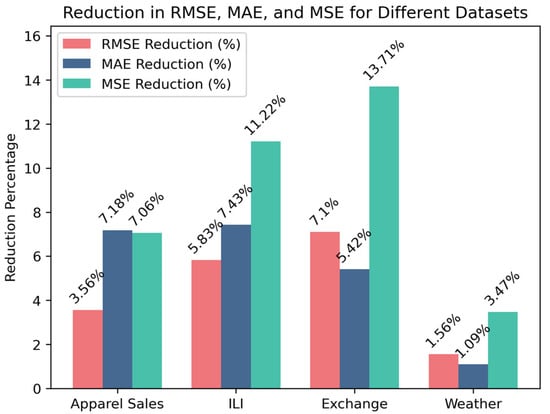
Figure 10.
Experimental results of MD–Autoformer after hyperparameter optimization on different datasets.
4. Discussion
This study proposes a time-series tailored multi-scale feature fusion network and develops the MD–Autoformer model based on an enhanced Autoformer architecture. By integrating multi-scale feature fusion and date–time encoding, the model significantly improves its capability to capture dynamic trends and seasonal patterns in data. Experimental results demonstrate that MD–Autoformer achieves average reductions of 22.23% in RMSE and 29.73% in MAE compared to the baseline Autoformer on the apparel sales dataset. Furthermore, MD–Autoformer exhibits robust predictive performance on public datasets spanning diverse domains including meteorology, finance, and disease epidemiology. Statistical significance analysis (p < 0.05) confirms the validity of the proposed methodology.
The following conclusions are drawn from the experiments conducted in this study:
- RH1: Ablation and comparative experiments demonstrated that incorporating date–time encoding enhanced the model’s ability to recognize periodic temporal patterns, thereby supporting RH1.
- RH2: The multi-scale feature fusion network improved Autoformer’s prediction accuracy by extracting both local and global temporal features. Ablation studies confirmed that this approach effectively reduced error accumulation in scenarios with multi-scale seasonality, supporting RH2.
- RH3: Statistical significance analysis (p < 0.05) revealed that combining date–time encoding with the multi-scale fusion network led to a statistically significant improvement in prediction performance, validating RH3.
- RH4: The TPE-based Bayesian hyperparameter optimization improved the prediction accuracy of MD–Autoformer across datasets from multiple distinct domains, thereby validating RH4.
The experimental results further reveal that the multi-scale feature fusion network based on multi-scale convolutions can effectively extract the key features of time series from different time scales, accurately capturing multi-level information from short-term fluctuations to long-term trends. Meanwhile, the introduction of date–time encoding enables the model to focus on the potential relationships between data and time, thereby enhancing its perception of dynamic trend changes. Combining with the Bayesian hyperparameter optimization method further improves the performance of the model.
We think that hybrid models have an edge in scenarios with high data volatility. Autoformer-based models, focusing on long-term seasonal trends, may generate overly smooth forecast curves, struggling to track sequence changes flexibly. So, we will explore combining simple neural networks with transformer-based models in future research. Based on our experimental results, we recommend using the MD–Autoformer for time-series forecasting with clear seasonality or periodicity, such as in fashion sales, power demand, and disease prediction.
In future work, we will continue to refine our methodology to enable its application in more complex prediction tasks (e.g., economic policies, and market sentiment) and enhance its adaptability to volatile data. This advancement aims to improve the reliability of our model for sophisticated applications such as stock risk prediction.
Author Contributions
Conceptualization, X.M. and H.Z.; formal analysis, X.M.; methodology, X.M.; resources, X.M. and H.Z.; supervision, H.Z.; validation, X.M.; writing—original draft, X.M.; writing—review and editing, X.M. and H.Z. All authors have read and agreed to the published version of the manuscript.
Funding
This research was funded by “Pioneer” and “Leading Goose” R&D Program of Zhejiang, grant number 2022C01220, 2025C01067.
Institutional Review Board Statement
Not applicable.
Informed Consent Statement
Not applicable.
Data Availability Statement
The original contributions presented in this study are included in the article. Further inquiries can be directed to the corresponding author.
Acknowledgments
This research benefited greatly from the contributions of Huaxiong Zhang, whose valuable revisions and feedback during the revision stage significantly improved the manuscript.
Conflicts of Interest
The authors declare no conflicts of interest. The funders had no role in the design of this study; in the collection, analyses, or interpretation of data; in the writing of the manuscript; or in the decision to publish the results.
Abbreviations
The following abbreviations are used in this manuscript:
| ILI | Influenza-Like Illness |
| MSFNN | Multi-scale Feature Fusion Network |
| DE | Date–Time Encoding |
References
- Waqas, M.; Humphries, U.W.; Hlaing, P.T.; Ahmad, S. Seasonal WaveNet-LSTM: A Deep Learning Framework for Precipitation Forecasting with Integrated Large Scale Climate Drivers. Water 2024, 16, 3194. [Google Scholar] [CrossRef]
- Torres, J.F.; Hadjout, D.; Sebaa, A.; Martínez-Álvarez, F.; Troncoso, A. Deep learning for time series forecasting: A survey. Big Data 2021, 9, 3–21. [Google Scholar] [PubMed]
- Tanaka, K.; Akimoto, H.; Inoue, M. Production risk management system with demand probability distribution. Adv. Eng. Inform. 2012, 26, 46–54. [Google Scholar]
- Staffini, A. Stock price forecasting by a deep convolutional generative adversarial network. Front. Artif. Intell. 2022, 5, 837596. [Google Scholar] [CrossRef]
- Ahmad, Z.; Bao, S.; Chen, M. DeepONet-Inspired Architecture for Efficient Financial Time Series Prediction. Mathematics 2024, 12, 3950. [Google Scholar] [CrossRef]
- Staffini, A. A CNN–BiLSTM Architecture for Macroeconomic Time Series Forecasting. Eng. Proc. 2023, 39, 33. [Google Scholar] [CrossRef]
- Hyndman, R. Forecasting: Principles and Practice, 3rd ed.; OTexts: Melbourne, Australia, 2021. [Google Scholar]
- Ristanoski, G.; Liu, W.; Bailey, J. A time-dependent enhanced support vector machine for time series regression. In Proceedings of the 19th ACM SIGKDD International Conference on Knowledge Discovery and Data Mining, Chicago, IL, USA, 11–14 August 2013; pp. 946–954. [Google Scholar]
- Cortez, P. Sensitivity analysis for time lag selection to forecast seasonal time series using neural networks and support vector machines. In Proceedings of the 2010 International Joint Conference on Neural Networks (IJCNN), Barcelona, Spain, 18–23 July 2010; pp. 1–8. [Google Scholar]
- Cerqueira, V.; Torgo, L.; Soares, C. Machine learning vs statistical methods for time series forecasting: Size matters. arXiv 2019, arXiv:1909.13316. [Google Scholar]
- Box, G.E.; Pierce, D.A. Distribution of residual autocorrelations in autoregressive-integrated moving average time series models. J. Am. Stat. Assoc. 1970, 65, 1509–1526. [Google Scholar]
- Zhao, J.; Zhang, C. Research on Sales Forecast Based on Prophet-SARIMA Combination Model. J. Phys. Conf. Ser. 2020, 1616, 012069. [Google Scholar]
- Wei, J.; Zhu, J.; Huang, C.; Tang, Y.; Lin, X.; Mao, C. A novel prediction model for sales forecasting based on grey system. In Proceedings of the 2016 IEEE 9th International Conference on Service-Oriented Computing and Applications (SOCA), Macau, China, 4–6 November 2016; pp. 10–15. [Google Scholar]
- Zhang, B.; Tseng, M.-L.; Qi, L.; Guo, Y.; Wang, C.-H. A comparative online sales forecasting analysis: Data mining techniques. Comput. Ind. Eng. 2022, 176, 108935. [Google Scholar] [CrossRef]
- Zhou, X.; Meng, J.; Wang, G.; Xiaoxuan, Q. A demand forecasting model based on the improved Bass model for fast fashion clothing. Int. J. Cloth. Sci. Technol. 2020. ahead-of-print. [Google Scholar]
- Thomassey, S. Sales Forecasting in Apparel and Fashion Industry: A Review; Springer: Berlin/Heidelberg, Germany, 2014. [Google Scholar]
- Li, Y.; Yang, Y.; Zhu, K.; Zhang, J. Clothing sale forecasting by a composite GRU–Prophet model with an attention mechanism. IEEE Trans. Ind. Inform. 2021, 17, 8335–8344. [Google Scholar]
- He, K.; Ji, L.; Wu, C.W.D.; Tso, K.F.G. Using SARIMA–CNN–LSTM approach to forecast daily tourism demand. J. Hosp. Tour. Manag. 2021, 49, 25–33. [Google Scholar]
- Xu, D.; Zhang, Q.; Ding, Y.; Zhang, D. Application of a hybrid ARIMA-LSTM model based on the SPEI for drought forecasting. Environ. Sci. Pollut. Res. 2022, 29, 4128–4144. [Google Scholar]
- Dave, E.; Leonardo, A.; Jeanice, M.; Hanafiah, N. Forecasting Indonesia exports using a hybrid model ARIMA-LSTM. Procedia Comput. Sci. 2021, 179, 480–487. [Google Scholar]
- Fan, D.; Sun, H.; Yao, J.; Zhang, K.; Yan, X.; Sun, Z. Well production forecasting based on ARIMA-LSTM model considering manual operations. Energy 2021, 220, 119708. [Google Scholar]
- Wu, H.; Xu, J.; Wang, J.; Long, M. Autoformer: Decomposition transformers with auto-correlation for long-term series forecasting. Adv. Neural Inf. Process. Syst. 2021, 34, 22419–22430. [Google Scholar]
- Pan, K.; Lu, J.; Li, J.; Xu, Z. A Hybrid Autoformer Network for Air Pollution Forecasting Based on External Factor Optimization. Atmosphere 2023, 14, 869. [Google Scholar] [CrossRef]
- Zhong, J.; Li, H.; Chen, Y.; Huang, C.; Zhong, S.; Geng, H. Remaining Useful Life Prediction of Rolling Bearings Based on ECA-CAE and Autoformer. Biomimetics 2024, 9, 40. [Google Scholar] [CrossRef]
- Ma, S.; He, J.; He, J.; Feng, Q.; Bi, Y. Forecasting air quality Index in yan’an using temporal encoded Informer. Expert Syst. Appl. 2024, 255, 124868. [Google Scholar]
- Silva, E.S.; Hassani, H.; Madsen, D.Ø.; Gee, L. Googling fashion: Forecasting fashion consumer behaviour using google trends. Soc. Sci. 2019, 8, 111. [Google Scholar] [CrossRef]
- Skenderi, G.; Joppi, C.; Denitto, M.; Cristani, M. Well googled is half done: Multimodal forecasting of new fashion product sales with image-based google trends. J. Forecast. 2024, 43, 1982–1997. [Google Scholar] [CrossRef]
- Wiener, N. Generalized harmonic analysis. Acta Math. 1930, 55, 117–258. [Google Scholar]
- Ouyang, D.; He, S.; Zhang, G.; Luo, M.; Guo, H.; Zhan, J.; Huang, Z. Efficient multi-scale attention module with cross-spatial learning. In Proceedings of the ICASSP 2023—2023 IEEE International Conference on Acoustics, Speech and Signal Processing (ICASSP), Rhodes Island, Greece, 4–10 June 2023; pp. 1–5. [Google Scholar]
- Zhou, H.; Zhang, S.; Peng, J.; Zhang, S.; Li, J.; Xiong, H.; Zhang, W. Informer: Beyond efficient transformer for long sequence time-series forecasting. In Proceedings of the AAAI Conference on Artificial Intelligence, Virtually, 2–9 February 2021; pp. 11106–11115. [Google Scholar]
- Li, S.; Jin, X.; Xuan, Y.; Zhou, X.; Chen, W.; Wang, Y.-X.; Yan, X. Enhancing the locality and breaking the memory bottleneck of transformer on time series forecasting. In Proceedings of the 32nd Conference on Neural Information Processing Systems (NeurIPS 2019), Vancouver, BC, Canada, 8–14 December 2019; Advances in Neural Information Processing Systems 32. Volume 7 of 20. [Google Scholar]
- Zeng, A.; Chen, M.; Zhang, L.; Xu, Q. Are transformers effective for time series forecasting? In Proceedings of the AAAI Conference on Artificial Intelligence, Washington, DC, USA, 7–14 February 2023; pp. 11121–11128. [Google Scholar]
- Ślusarczyk, D.; Ślepaczuk, R. Optimal Markowitz Portfolio Using Returns Forecasted with Time Series and Machine Learning Models; Working Papers 2023-17; Faculty of Economic Sciences, University of Warsaw: Warsaw, Poland, 2023. [Google Scholar]
- Kashif, K.; Ślepaczuk, R. Lstm-arima as a hybrid approach in algorithmic investment strategies. arXiv 2024, arXiv:2406.18206. [Google Scholar]
- Michańków, J.; Sakowski, P.; Ślepaczuk, R. Hedging Properties of Algorithmic Investment Strategies using Long Short-Term Memory and Time Series models for Equity Indices. arXiv 2023, arXiv:2309.15640. [Google Scholar]
- Stefaniuk, F.; Ślepaczuk, R. Informer in Algorithmic Investment Strategies on High Frequency Bitcoin Data. arXiv 2025, arXiv:2503.18096. [Google Scholar]
- Kryńska, K.; Ślepaczuk, R. Daily and Intraday Application of Various Architectures of the LSTM model in Algorithmic Investment Strategies on Bitcoin and the S&P 500 Index. Working Papers of Faculty of Economic Sciences, Univeristy of Warsaw, WP 25/2022 (401). Available online: https://papers.ssrn.com/sol3/papers.cfm?abstract_id=4628806 (accessed on 16 February 2025).
- Roszyk, N.; Ślepaczuk, R. The Hybrid Forecast of S&P 500 Volatility ensembled from VIX, GARCH and LSTM models. arXiv 2024, arXiv:2407.16780. [Google Scholar]
- Lai, G.; Chang, W.-C.; Yang, Y.; Liu, H. Modeling long-and short-term temporal patterns with deep neural networks. In Proceedings of the 41st International ACM SIGIR Conference on Research & Development in Information Retrieval, Ann Arbor, MI, USA, 8–12 July 2018; pp. 95–104. [Google Scholar]
- Zulfiqar, M.; Gamage, K.A.; Kamran, M.; Rasheed, M.B. Hyperparameter optimization of bayesian neural network using bayesian optimization and intelligent feature engineering for load forecasting. Sensors 2022, 22, 4446. [Google Scholar] [CrossRef]
- Jiang, B.; Gong, H.; Qin, H.; Zhu, M. Attention-LSTM architecture combined with Bayesian hyperparameter optimization for indoor temperature prediction. Build. Environ. 2022, 224, 109536. [Google Scholar]
- Du, L.; Gao, R.; Suganthan, P.N.; Wang, D.Z. Bayesian optimization based dynamic ensemble for time series forecasting. Inf. Sci. 2022, 591, 155–175. [Google Scholar]
- Snoek, J.; Larochelle, H.; Adams, R.P. Practical bayesian optimization of machine learning algorithms. In Proceedings of the Advances in Neural Information Processing Systems, Lake Tahoe, NV, USA, 3–6 December 2012; pp. 2951–2959. [Google Scholar]
Disclaimer/Publisher’s Note: The statements, opinions and data contained in all publications are solely those of the individual author(s) and contributor(s) and not of MDPI and/or the editor(s). MDPI and/or the editor(s) disclaim responsibility for any injury to people or property resulting from any ideas, methods, instructions or products referred to in the content. |
© 2025 by the authors. Licensee MDPI, Basel, Switzerland. This article is an open access article distributed under the terms and conditions of the Creative Commons Attribution (CC BY) license (https://creativecommons.org/licenses/by/4.0/).