Article

MOIRA-UNIMORE Bearing Data Set for Independent Cart Systems

1
Department of Engineering Sciences and Methods, University of Modena and Reggio Emilia (UNIMORE), Via Amendola 2, Pad-Morselli, 42122 Reggio Emilia, Italy
2
Tetra Pak Packaging Solutions, 41123 Modena, Italy
*
Author to whom correspondence should be addressed.
Appl. Sci. 2025, 15(7), 3691; https://doi.org/10.3390/app15073691
Submission received: 7 February 2025 / Revised: 20 March 2025 / Accepted: 24 March 2025 / Published: 27 March 2025
(This article belongs to the Special Issue Fault Diagnosis and Detection of Machinery)

Abstract

:
This paper introduces a comprehensive and publicly accessible data set from an experimental study on an independent cart system powered by linear motors. The primary objective is to advance research in machine health monitoring, predictive maintenance, and stochastic modeling by providing the first data set of its kind. Vibration signals were collected using sensors placed along the track, alongside key system variables such as cart position, following error, speed, and set current. Experiments were conducted under a wide range of operating conditions, including different fault types, fault severities, cart speeds, and fault orientations, for both single-cart and multi-cart configurations. The data set captures the relationship between vibration signatures, system variables, and fault characteristics across diverse speed profiles. The data set includes inner race (IR) and outer race (OR) faults in both the top and bottom bearings, with fault severities of 0.25 mm, 0.5 mm, 1.0 mm, and 1.5 mm in width. Eight different types of experiments were performed, classified based on the number of carts used, the section of the guide rail traversed, and the type of movement exhibited. Each experiment was conducted at two distinct nominal speeds of 1000 mm/s and 2000 mm/s, with acquisition durations ranging from 30 s to 2 min. Many experiments included multiple realizations to ensure statistical reliability. Data were recorded at a sampling frequency of 50 kHz with a resolution of 24 bits. For single-cart experiments, 5 system variables were captured, while for three-cart experiments, 15 system variables were recorded along with nine vibration channels. The total data set is approximately 400 GB, offering an extensive resource for data-driven research. Independent cart systems present unique challenges such as non-synchronous operation, speed reversals, and modularity, with each cart containing multiple bearings. In industrial applications where hundreds of carts may operate simultaneously, monitoring a large number of bearings becomes highly complex, making fault identification and localization particularly difficult. Unlike conventional rotary systems, where bearings are fixed around a rotating shaft, independent cart systems involve bearings that both rotate and translate along the track. This fundamental difference makes existing data sets and methodologies inadequate, emphasizing the need for specialized research. By addressing this gap, this work provides a critical resource for benchmarking and developing novel algorithms for fault diagnosis, signal processing, and machine learning in industrial transport applications. The outcomes of this study lay the foundation for future research in the condition monitoring of linear motor-driven transport systems.

1. Introduction

The advancement in linear motors has led to the emergence of novel independent cart systems [1,2,3,4] that have overcome the limitations of traditional transport systems, such as conveyors, rollers and chain-driven mechanisms, which rely heavily on gears, chains, and belts. These conventional systems often require numerous mechanical components distributed along the entire transport pathway, including motors, pulleys, rollers, and sprockets, to achieve transportation. The interconnected nature of these systems introduces significant mechanical complexity, making it challenging to monitor, maintain, and optimize their operation. In addition, the need for constant lubrication, frequent adjustments, and the inherent wear and tear of moving parts increase downtime and maintenance costs. Traditional systems also exhibit inefficiencies such as high friction losses, energy wastage, and reduced accuracy in motion control. These limitations make it difficult for such systems to adapt to modern industrial demands that require high-speed, precise, and flexible transportation solutions.
Independent cart technology addresses these challenges by using linear motors to independently move carts along a predetermined track. The carts are designed with permanent magnets, while the linear motors are equipped with coils that generate a magnetic field, enabling synchronized movement with the changing magnetic pattern. Using magnets, independent cart technology achieves precise control over motion with a minimal number of mechanical components compared to conventional conveyor systems. The current study differs significantly from the systems described in [3,4] in two key aspects. First, the configuration of the system in [3,4] involves a guide rail directly attached to the motor module, while the current study examines a system in which the guide rail is positioned in parallel to the motor modules. This difference in mechanical configuration results in distinct dynamic behaviors and vibration characteristics. Second, the outer race of the bearing in [3,4] is made of plastic, which influences the propagation of faults and vibration patterns differently compared to the steel bearings used in the current study. A notable feature of this technology is its frictionless propulsion mechanism, which eliminates physical contact between the cart and the linear motor coils. This significantly minimizes the wear and tear on individual parts and streamlines the transportation or movement process. This efficient solution reduces energy consumption and operational costs and enables quick start and stop capabilities without compromising movement control, providing a distinct advantage over traditional conveyors. The reduction in mechanical complexity also allows for improved condition monitoring and fault detection, enhancing the reliability and longevity of the system. Additionally, this feature increases system throughput while mitigating risks, such as material loss or damage associated with stopping and starting operations. The versatility of independent cart technology allows for precise and seamless manipulation and movement across a wide range of speeds, making it highly suitable for various industrial applications. Its ability to adapt to diverse operational requirements further enhances productivity and offers potential optimization of industrial processes. While this study focuses on the development of a novel data set for bearing faults in independent cart systems, recent advances in related fields provide valuable information. For example, Ref. [5] introduces a lightweight model for the detection of defects in ultrasonically welded wire terminations, highlighting the importance of efficient fault detection methodologies. Similarly, Ref. [6] revisits the historical development of rolling bearing life formulas, offering a comprehensive perspective on bearing performance evaluation. Furthermore, Ref. [7] explores the simulation of thermal conductivity in bearing assemblies, emphasizing the role of thermal effects in bearing behavior. Although these studies address different aspects of fault detection and bearing performance, they collectively underscore the importance of innovative approaches in condition monitoring and predictive maintenance. Despite these advantages, independent cart systems introduce unique challenges for fault diagnosis due to their translational motion, speed variability, and modularity. Traditional fault detection techniques developed for rotary systems may not be directly applicable, necessitating novel approaches that leverage advanced predictive maintenance strategies.
The latest progress in predictive maintenance and fault diagnosis has notably enhanced the surveillance of industrial equipment through the use of machine learning and deep learning techniques [8,9,10]. Approaches like deep convolutional networks, bidirectional LSTM (Bi-LSTM), and deep belief networks (DBNs) have been investigated for applications involving rolling element bearings and rotating machinery, attaining cutting-edge accuracy in fault detection and RUL forecasting [11,12,13]. Moreover, to tackle challenges in cross-domain fault classification, deep transfer learning and domain adaptation (DA) methodologies have been introduced [14,15,16]. Nonetheless, the use of these sophisticated methods for autonomous cart systems has not been extensively studied, with current research predominantly centered on standard rotary machinery. Additionally, there has been growing interest in cluster-based techniques for unsupervised and semi-supervised fault diagnosis, which enhance feature selection, class separability, and novelty detection [17,18,19]. Tactics like affinity propagation (AP), density-based spatial clustering (DBSCAN), and subspace clustering have effectively been utilized in rotating machinery for feature extraction and identification [20,21,22,23]. Despite their success, these techniques must be tailored to suit independent cart systems because of their highly variable, non-synchronous movement and changes in speed. Additionally, one major obstacle in condition monitoring is the presence of imbalanced data sets, which can significantly impact the accuracy of classifiers. Methods such as Cluster-MWMOTE [24] and SMOTE with PCA [25] have been suggested to counter bias in fault classification, especially in cases where some fault conditions are more prevalent. Considering that independent cart systems may have multiple bearings per cart, data set imbalances and class representation can be decisive issues in developing reliable fault detection algorithms. To improve automated fault detection, multisensor fusion has been investigated within industrial condition monitoring. Techniques such as frequency domain multilinear principal component analysis (FDMPCA) [26] and graph-based manifold learning [27] have proven to be effective when integrating vibration, acoustic and various sensor modalities for enhanced fault diagnosis. Despite this, independent cart systems add further complexity due to interactions among multiple bearings, guide rails, and system variables. This complexity may necessitate new multisensor fusion approaches for efficient fault detection.
Despite advances in fault detection methodologies, their practical implementation in independent cart systems remains challenging due to the complex motion dynamics of the system and the economic consequences of prolonged downtime. Given the substantial initial investment required for these systems, uninterrupted operation is critical for economic feasibility. However, unexpected failures can severely impact productivity and profitability. Therefore, continuous condition monitoring is essential to prevent costly breakdowns, ensure early fault detection, reduce downtime, and protect long-term operational efficiency.
Although independent cart systems are increasingly replacing traditional conveyor belt systems, research on condition monitoring for such systems remains limited. This gap is largely due to confidentiality concerns, often enforced by non-disclosure agreements, which restrict the sharing of vibration, acoustic, or other relevant data. Consequently, there are no public repositories or databases for conducting condition monitoring studies on independent cart systems. To the best of the authors’ knowledge, there is almost no academic research available in this domain. This study addresses this critical gap by providing a comprehensive analysis and a publicly accessible data set that serves as a foundational resource for future research in this emerging field. The unique contribution of this paper lies in its focus on independent cart systems, a topic that has been largely overlooked, and its provision of valuable data and insights that were previously unavailable. These factors underscore the significance and novelty of this work, making it a strong candidate for publication.
Furthermore, the inherent challenges associated with the condition monitoring of independent cart systems further underscore the need for this research. These systems are highly non-synchronous, with speed variations ranging from a few millimeters per second to several meters per second. For example, the system under study can achieve cart speeds of up to 4 m per second. Moreover, independent cart systems allow for speed reversal, enabling changes in direction. The complexity is further compounded by the modular nature of these systems, where each cart contains multiple bearings. For example, the system under study includes three bearings per cart, and with the addition of each cart, the total number of bearings increases by three. In practical industrial applications, where hundreds of carts may be in operation, this translates into monitoring the condition of hundreds of bearings. This makes fault identification and location significantly more challenging.
Another significant motivation for this research lies in the fundamental differences between independent cart systems and conventional rotary machinery, which form the basis for most publicly available rolling element bearing data sets. In conventional systems, the bearings are fixed around a rotating shaft, and most data sets, such as those referenced in [28,29,30,31], are designed for fault detection in these stationary configurations. Throughout the years, numerous publicly accessible data sets have been developed to assist in diagnosing faults in rotary systems. Notable examples include the XJTU-SY data set for rolling bearings [32], the SEU gearbox data set aimed at detecting gear faults [33], and the Airbus PHM challenge data set [34], which is dedicated to prognostics and health management. These data sets offer invaluable tools for assessing the condition of conventional machinery. Nonetheless, they fail to tackle the specific challenges presented by independent cart systems, where the movement involves both rotational and translational dynamics along a track. Unlike rotary machinery, where fault progression is primarily influenced by rotational dynamics, independent cart systems introduce a complex interaction between translational motion, system variability, and fault propagation. This fundamental difference makes independent cart systems depart significantly from standard data sets and methodologies, emphasizing the need for specialized research in this area.
The data set presented in this study offers significant benefits in advancing research on condition monitoring and predictive maintenance for independent cart systems. It provides a comprehensive and publicly accessible resource that captures the unique dynamics of these systems, including vibration signatures, internal system variables, and fault characteristics in various speed profiles. This enables researchers to develop and benchmark novel algorithms for fault diagnosis, signal processing, and machine learning in industrial transport applications. However, there are potential difficulties in applying this data set to other industrial systems. First, the data set is specifically tailored to independent cart systems with linear motors, which differ fundamentally from conventional rotary systems in terms of mechanical configuration and operational dynamics. Systems with different designs or bearing materials may exhibit different vibration patterns and fault behaviors, which limits the direct applicability of the data set. Second, the data set assumes a specific set of parallel guide rails and steel bearings, which may not align with the configurations of other industrial systems. Finally, the reliance of the data set on specific fault types and severities may require adaptation or extension to address the unique fault scenarios encountered in other systems.

Key Contributions

  • This is the first publicly available data set specifically designed for bearing fault diagnosis in independent cart systems.
  • A comprehensive system description is given, including experimental setup, experimental configurations, sensor configurations, and fault injection methodology.
  • It is a multisensor data set capturing vibration signals and system variables under varied operating conditions.
  • The data set is structured to support future research in condition monitoring, feature extraction, and predictive maintenance.
The organization of this paper is as follows. Section 2 provides a comprehensive description of the experimental system, including its key components and associated parameters. Section 3 presents the experimental campaign, detailing the phases of data collection, fault injection strategies, and improvements made over time. Section 4 outlines the methodology for injecting controlled bearing defects, describing the fault injection procedures. Section 5 covers the experimental data acquisition process, explaining the configurations and protocols used to collect the data set. Section 6 introduces the data set repository, describing the structure of the collected data and how it is organized for further analysis. Section 7 presents feature extraction and preprocessing techniques, followed by Section 8, which discusses data analysis and visualization. Section 9 summarizes the findings and their implications, serving as the conclusion. Appendix A explains the file and variable naming conventions and provides details on exporting data files into the desired formats for further analysis. Finally, the references are included in a separate section.

2. Description of the Experimental Setup

This study used an independent cart system based on the Extended Transport System (XTS) [1]. The system comprises several key components (Figure 1 and Figure 2): a fixed set of linear motors (stators), movable carts (movers) equipped with permanent magnets, a guide rail running parallel to the fleet of linear motors that enables the carts to glide, a set of five strategically placed vibration sensors, an analog input acquisition system, a control circuit for programming and motion profiling of the movable carts, and software for real-time control and data handling. In this work, our primary focus is on the mechanical aspects of the system that directly influence the vibration signatures and system variables.

2.1. Linear Motor Modules

For the experimental setup, we use a closed loop track configuration, consisting of ten linear motor modules—eight straight modules and two 180-degree clothoid (curved) modules—as illustrated in Figure 1. Each straight module has a length of 250 mm, while each curved module spans 500 mm. This configuration results in a total track length of 3000 mm, enabling the carts to traverse a complete loop under varying test conditions. The track is divided into four main sections, each serving a specific purpose and contributing uniquely to the system’s dynamics.

2.1.1. Upper Straight Modules Section

This section extends between the absolute positions of 750 mm and 1750 mm and is located in the upper part of the system. A notable feature of this module is the presence of a lock, which allows the addition or removal of carts from the guide rail. This lock introduces a physical discontinuity in the track, resulting in distinctive impulsive vibration signals caused by bearing impacts as the cart traverses this area. Consequently, the vibration signals captured in this section differ significantly from those in the lower straight section, providing valuable information on the system response to irregularities in the track.

2.1.2. Curved Modules

The track includes two curved modules located on the left and right sides. The first curved module connects the absolute positions of 250 mm and 750 mm, while the second spans the positions between 1750 mm and 2250 mm. These modules introduce additional complexities to the cart’s motion, such as varying inertial forces due to changes in direction and speed. The curved sections play a critical role in evaluating the system’s performance under nonlinear motion profiles.

2.1.3. Lower Straight Modules Section
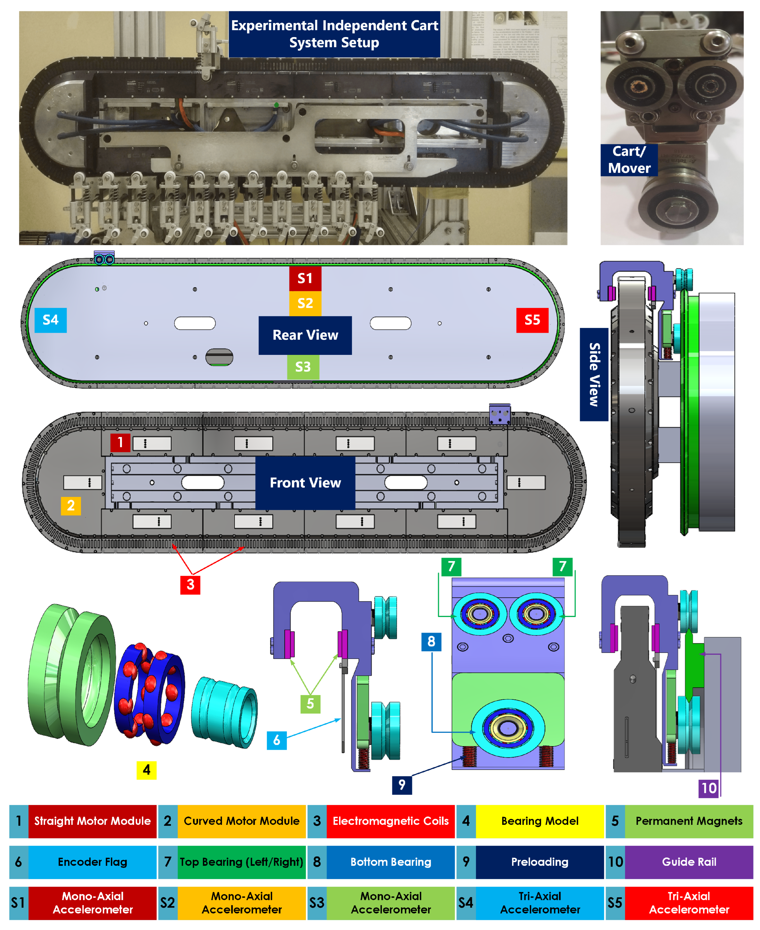
Situated in the lower part of the system, this straight motor module covers the absolute positions between 2250 mm and 3000 mm. Unlike the upper section, this part of the track lacks physical discontinuities, resulting in smoother vibration signals. The comparison of signals between the upper and lower straight sections highlights the impact of track features, such as locks, on the system dynamics.

2.2. Cart/Mover

Each cart in the system is equipped with four primary components that contribute to its functionality and precise motion control:
  • Magnetic Plates: Each cart has a pair of magnetic plates, with five magnets on each plate. These magnets define the cart’s length along the track as 50 mm and interact with the linear motor’s magnetic field to enable controlled motion.
  • Encoder Flag: The cart is equipped with an encoder flag that provides real-time feedback on its actual position along the track. This ensures precise tracking and synchronization of the cart movement with the overall system.
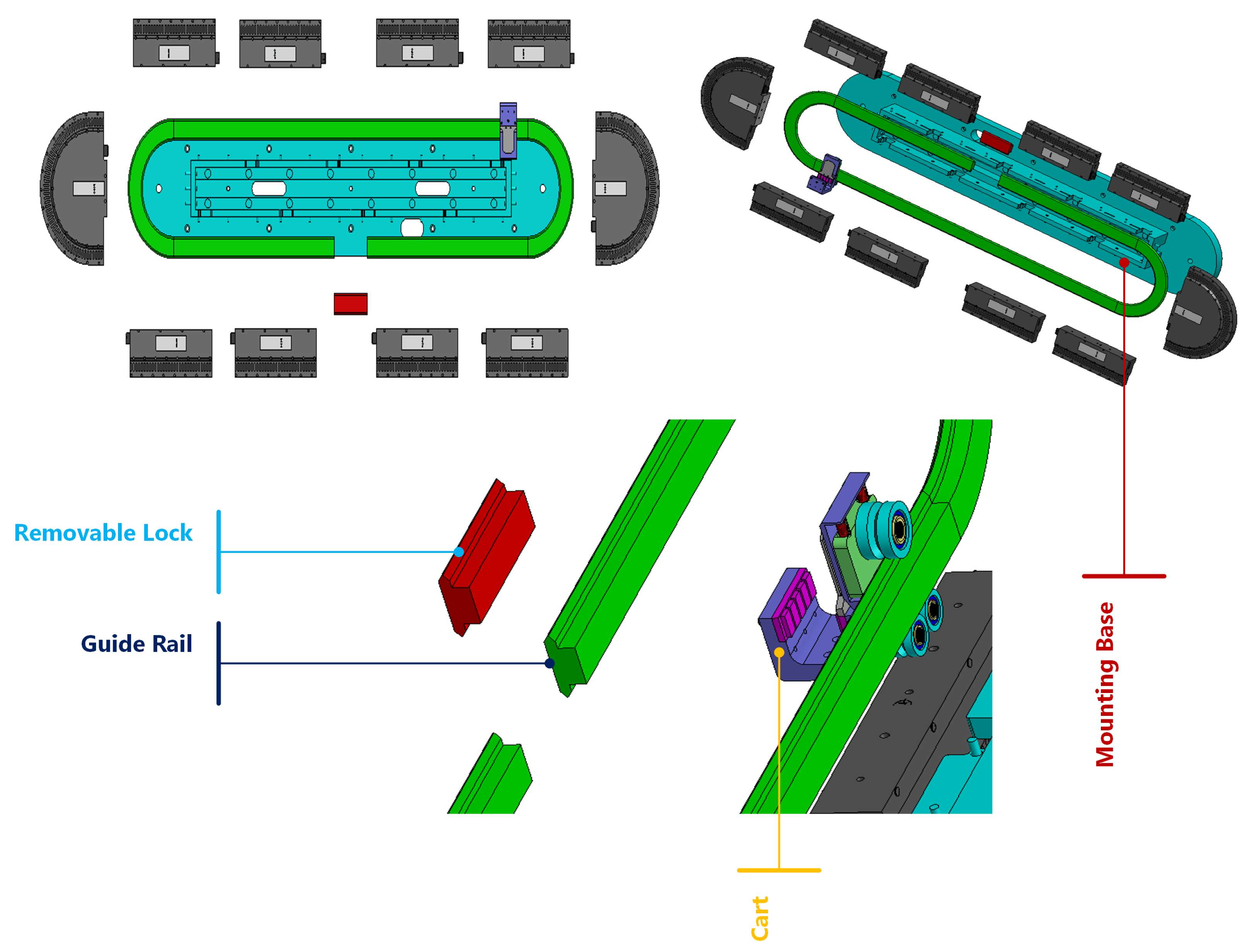
  • Rolling Element Bearings: The cart is supported by three rolling element bearings arranged to maintain stability and proper alignment with the guide rail. The configuration includes two smaller, identical bearings positioned on the top and one larger bearing at the bottom. This arrangement secures the cart to the guide rail, ensuring smooth and stable movement. All bearings share the same design characteristics: they feature two rows of deep grooves on the inside and a V-shaped groove on the outer race that matches the profile of the guide rail. In this setup, the bearing’s outer race rotates while the inner race remains stationary. The dimensions and parameters of the bearings used in the experimental setup are detailed in Table 1, providing essential information to understand the mechanical characteristics of the system. The bearings used in this study are part of the GFX Hepco guidance systems for Beckhoff XTS. Detailed specifications regarding the bearing materials, including the types of materials in contact (e.g., steel-on-steel), are provided in the manufacturer’s documentation [35]. This information is critical for understanding the material interactions and operational conditions of the bearings during the experiments.
  • Preloading Mechanism: A spring-like preload mechanism is incorporated to adjust grip and evenly distribute forces across the top and bottom bearings. This mechanism improves stability and provides the necessary radial forces for the bearings, ensuring consistent contact with the guide rail under varying load conditions.
Table 1. Bearing dimensions and parameters.
Bearing TypeNumber of RowsNumber of BallsBall Diameter (mm)OR Diameter (mm)IR Diameter (mm)Pitch Diameter (mm)
Top Bearing27, 73.952510.7514.70
Bottom Bearing27, 75.553414.6020.15
In addition, the cart can be customized to attach an end effector for transporting payloads, provided the weight remains within the maximum allowable limits. Furthermore, since the cart magnets do not come into direct contact with the motor coils but instead interact through a magnetic field, friction and wear are significantly minimized during operation. Together, these features ensure that the cart delivers reliable, efficient, and precise motion while reducing maintenance requirements, making the system highly suitable for demanding industrial applications. Although some defects, such as chipped magnets, have been reported, the primary focus of condition monitoring in this study is bearing faults, as they represent the most stressed components in this experimental configuration.

2.3. Accelerometers

The experimental setup included five vibration sensors (see Table 2) strategically placed to monitor the system’s vibration signature. Two triaxial accelerometers were mounted on sections of the guide rail parallel to each of the two curved modules (Left: 356B21, Right: 356A02). In addition, two monoaxial accelerometers (353B18) were installed on the guide rail sections near the upper and lower straight modules, approximately midway along the track. Another monoaxial accelerometer (VSP001) was positioned on an aluminum rod directly attached to the guide rail on the upper side of the system, located midway along the straight section. This sensor arrangement ensured comprehensive coverage for capturing vibration signals across different sections of the track.

2.4. Acquisition System

For data acquisition, we used the Beckhoff ELM3602-0002 module (Beckhoff Automation GmbH & Co., Verl, Germany), a high-performance analog input terminal specifically designed for IEPE (Integrated Electronics Piezo-Electric) sensors and accelerometers. This module features 24-bit resolution, ensuring precise and accurate measurements, and supports sampling rates of up to 50 ksps (kilo samples per second). The high resolution and fast sampling capability make it ideal for capturing detailed vibration signals and dynamic responses critical for condition monitoring and fault diagnosis in industrial applications. This advanced hardware ensures that even subtle changes in vibration signatures are effectively recorded, providing a robust foundation for data analysis and modeling.

2.5. Motion Control and System Programming

The programming for motion control and data acquisition was carried out using the TwinCAT 3 programming environment, which offers advanced tools for real-time automation and control. However, the technical details of the programming process are beyond the scope of this study, as the primary focus is on the recorded data set itself. This study aims to present the data along with the experimental conditions under which they were collected, rather than delving into the intricacies of the motion control programming or the data acquisition configurations. The emphasis is placed on the unique data set and the methodologies used to create it, ensuring it serves as a valuable resource for researchers and practitioners.

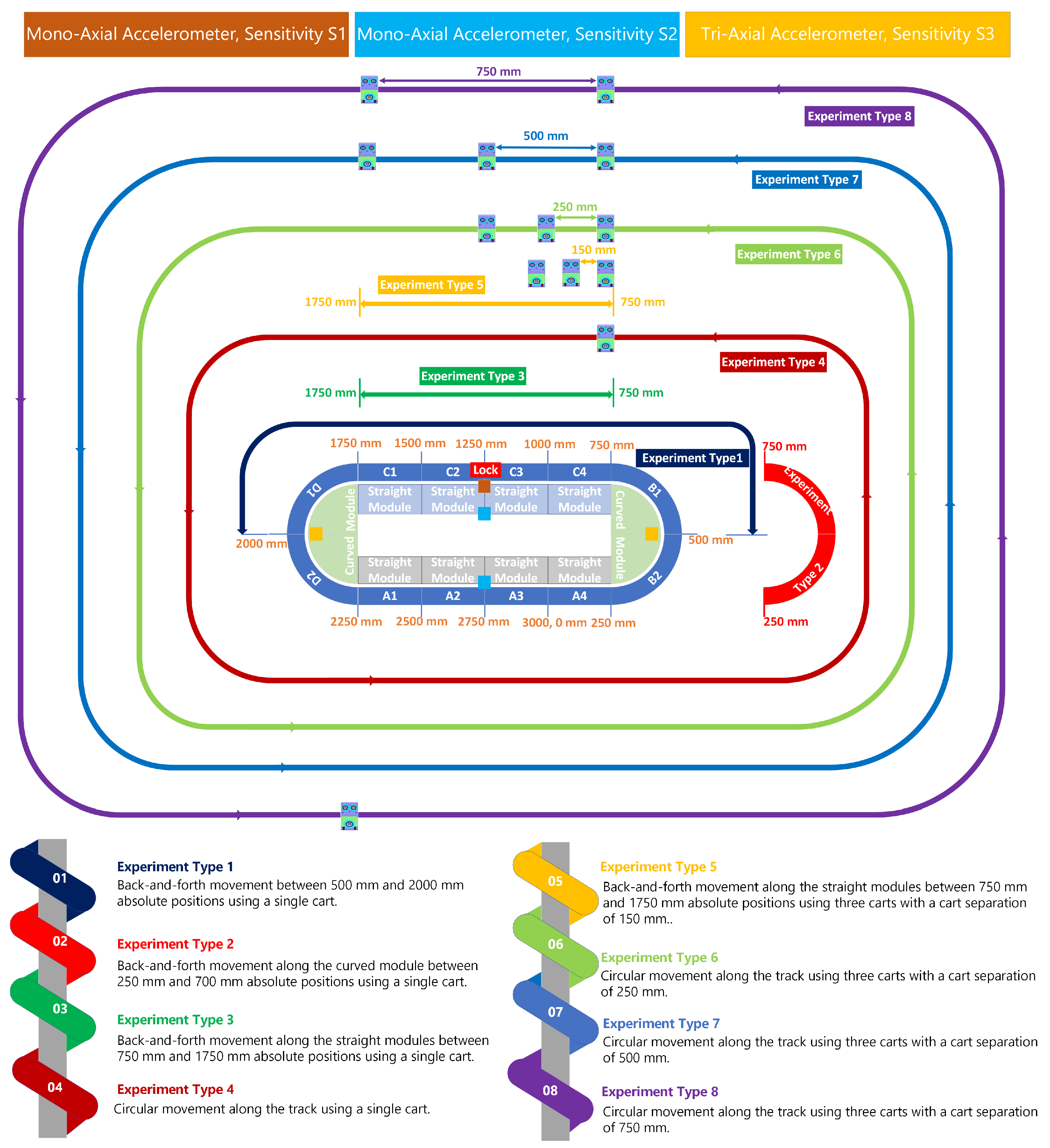
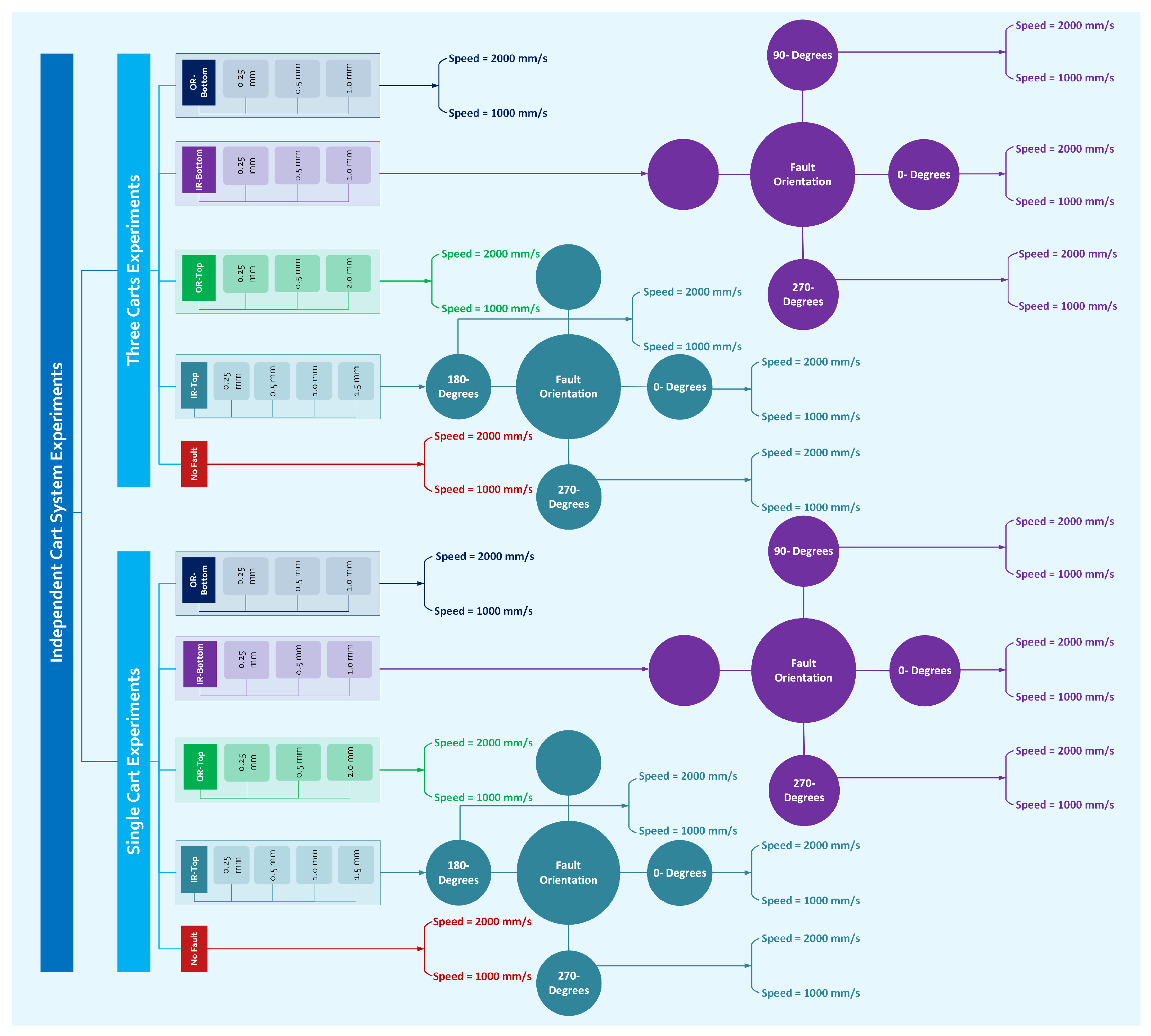
3. Experimental Campaign

In this study, data collection was conducted over several months, involving multiple iterations of experiments. Initially, various test runs were performed, and some data sets were discarded due to inadequate fault injection, insufficient resolution of the data acquisition system, or weak vibration signals that did not provide meaningful insights. Additionally, different experimental conditions were explored, including variations in the number of carts and loading mechanisms. Based on these observations, the data acquisition system was eventually upgraded to a 24-bit resolution with a 50 kHz sampling frequency. Faults were later introduced using laser-based precision techniques to ensure repeatability and accuracy in the fault injection process. The experimental campaign could be categorized into two main aspects, fault injection and data acquisition under varying conditions, including different cart configurations, speed profiles, fault sizes, and fault locations. Fault injection experiments were further classified into two types: non-invasive fault injection, where the bearings remained intact, and invasive fault injection, where the bearings were disassembled before introducing faults. A summary of the experimental phases, challenges encountered, and improvements implemented is presented in Table 3. The fault injection methodology is discussed in detail in the next section.

4. Fault Injection Methodology
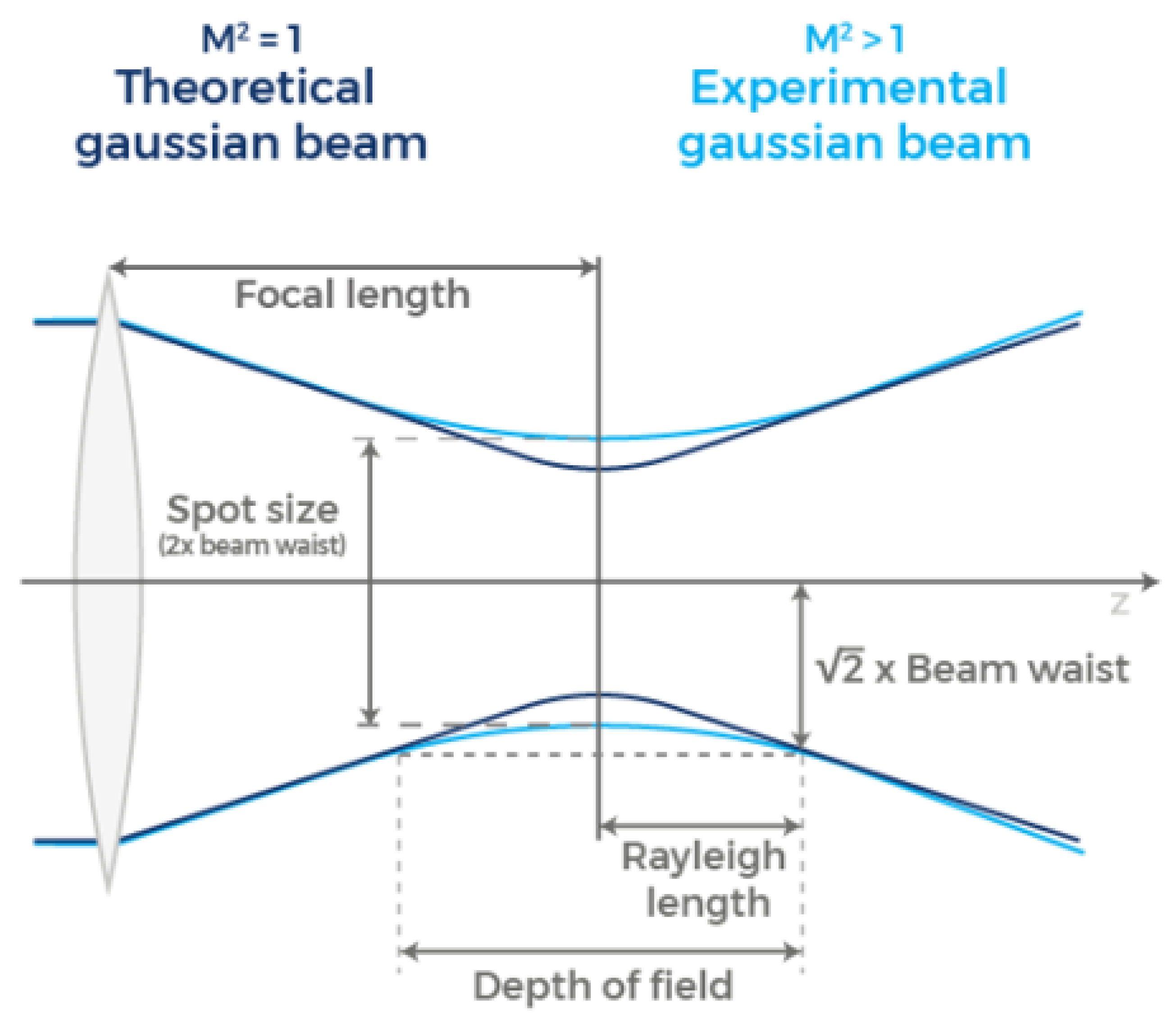
Fault injection was performed using two methods: non-disassembled and fully dismantled bearings. Initially, faults were introduced using a Lab-available drill mill without dismantling the bearings. However, the limited maneuverability of the drill mill head, the proximity of the bearing races, and the inherent rigidity of the stainless steel material made it difficult to create significant faults. As a result, the faults were of an incipient nature and did not fully encompass the grooves. To overcome this limitation, a picosecond laser (EKSPLA Atlantic 50) was used to create controlled faults without dismantling. The EKSPLA Atlantic 50 generated a Gaussian beam profile at an infrared (IR) wavelength of 1064 nm (see Figure 3). This laser source produces ultrashort pulses in the picosecond range, enabling the precise ablation of both the inner and outer races by creating accurately shaped grooves. Notably, this process is not limited by the hardness of the material being processed. The diameter of the laser beam at the focal point is set at ϕ 10 μm, measured at the 1 / e 2 intensity level. A dedicated optical path for the IR wavelength ensures that the laser beam is efficiently delivered from the source to the scanning head. The system employs a Raylase SuperScan IV galvanometric scanner coupled with an 80 mm F-theta lens, providing a square working area with a side length of 39 mm. Movements outside this scanning area are facilitated by the translation of a stage in the X and Y directions, on which the bearings to be processed are mounted. Additionally, the Z-axis translation ensures that the bearings are processed at the correct focal height. The entire setup, located in the BrightLab laboratory of the DISMI Department, is illustrated in Figure 4. Preliminary tests were conducted to assess the material’s response to infrared radiation. These tests were crucial for identifying and defining the optimal process parameters to achieve damage with specific geometry, dimensions, and prescribed depth. The laser parameters used in the process are summarized in Table 4. Although effective, this method presented challenges, particularly in damaging the inner and outer races. The first challenge stemmed from the shielding effect of the bearing components, which obstructed laser radiation and limited defect creation along the full axial extension. The second involved the difficulty of forming grooves with predetermined depths on inclined surfaces (Figure 5).
To address these limitations and ensure consistent damage results across various bearing components—comparable to those achieved in preliminary planar tests—an assessment of the allowable depth of focus was necessary. Specifically, by assuming a beam quality factor M 2 of 1.5 and a laser beam diameter (measured at 1 / e 2 intensity) of D 0 = 14 mm on the lens, the following calculations were performed:
  • Rayleigh length z f , as the distance from the beam waist, where the beam radius is increased by a factor of the 2 :
z f = π D 0 2 2 M 2 λ 100 μ m
  • Depth of field (D.O.F.) as the distance on either side of the beam waist, D 0 , over which the beam diameter grows by 5%
D . O . F . = ± 0.08 π D 0 2 M 2 λ 118 μ m
The relatively small depth of field (D.O.F.) of our laser, calculated at 118 μ m, made it impossible to damage the bearing components in a single laser pass. As a result, a multi-pass approach was adopted. This method involves focusing the laser beam on a specific target area of the component to be damaged. The process is defined by achieving the desired depth in the focused region, while areas outside the focal zone remain untreated due to insufficient energy deposition for proper material ablation. Consequently, the processing area is confined to a rectangle with a height equal to the previously calculated depth of field. Regions outside this height remain unprocessed because the laser beam is out of focus. To achieve the required depth incrementally, the height of the galvanometric head was adjusted, and the X position was compensated for by advancing the XY table. By refocusing the laser on a lower area, additional ablation could be performed. This process was repeated continuously until the desired damage geometry was achieved, with a depth tolerance of ± 0.15 mm from the nominal shape. To address the limitations discussed earlier, the bearings were fully disassembled. This allowed individual components to be exposed, enabling precise and controlled fault injection. Disassembly eliminated obstructions, such as balls between the inner and outer races, which previously hindered access to the target areas. As a result, more accurate and well-defined flat-bottom grooves were created using the multi-pass strategy described above. The final fault dimensions and geometry were characterized using an optical microscope (Model: Nikon LV100ND). By adjusting the depth of focus, detailed measurements were obtained. Further methodological details on fault characterization can be found in [36]. Figure 6 shows a microscopic view of some faults created without disassembling the bearings. As can be observed, the depth of the faults varies inconsistently, a result of the challenges previously discussed.

5. Experimental Data Acquisition

The acquisition system for this study employs five accelerometers, comprising monoaxial and triaxial types, categorized into three groups according to the number of channels and the levels of sensitivity. A monoaxial accelerometer (Sensitivity S1), with a sensitivity of 100 mV/g, is mounted midway along the upper straight section of the system. This sensor is not directly attached to the guide rail; instead, it is mounted on an aluminum rod securely fastened to the guide rail. Two monoaxial accelerometers (Sensitivity S2), each with a sensitivity of 10 mV/g, are positioned midway along the upper and lower sections of the track. In addition, two triaxial accelerometers are mounted on the left and right curved modules, each channel offering a sensitivity of approximately 10 mV/g. These sensors are carefully mounted at important points along the track to capture vibration signals effectively. In addition to vibration data, system variables such as cart position, speed, following error, and set current are recorded for each cart, enriching the data set for advanced condition monitoring and fault diagnostics. Detailed specifications for these accelerometers can be found on the manufacturer’s website using the part numbers provided in the system description section.
The data acquisition strategy was carefully designed to collect complete data sets from an independent cart transport system operating under a variety of fault conditions, speed profiles, and cart configurations. The experiments were organized into two main categories: single-cart and three-cart fleet experiments. Each category was further divided into four distinct experimental types, covering variations in fault locations, fault orientations, fault severities, motion patterns, and operating speeds. These experimental classifications aimed to comprehensively capture the dynamic behavior of the system in various operational scenarios as illustrated in Figure 7. This structured approach ensures that the data accurately represent the interplay of system variables and fault characteristics in different configurations. The data were acquired at two cart speeds: 1000 mm/s and 2000 mm/s. The speed of 1000 mm/s was defined as the minimum speed at which vibration signals become clearly observable and measurable. Below this threshold, the vibration signals were found to be too weak or inconsistent for reliable analysis. The speed of 2000 mm/s was chosen, as it represents half of the system’s maximum operational speed. This allows for a comparative analysis of how vibration signals change as the speed doubles, providing insights into the relationship between speed and vibration behavior. Both speeds are within the operational limits of the experimental setup, ensuring that the system can reliably achieve and maintain these speeds without compromising data quality or experimental integrity.
Experiments were conducted both with and without bearing faults to ensure a comprehensive analysis. For small bearings, faults were always introduced on the top right bearing, and only one bearing was faulty at a time. Additionally, across all experiment types, either one of the top bearings or the bottom bearing carried an inner race (IR) or outer race (OR) fault, ensuring controlled and consistent fault conditions. The same cart was used for all tests, both in faulted and non-faulted conditions. To maintain experimental consistency, the same speed profile and program settings were applied for each type of experiment. The development of the test setup was an iterative process over several months, incorporating refinements such as improved fault injection techniques and data acquisition enhancements. These aspects are detailed in the experimental campaign section, which outlines the phases of data collection, improvements made, and the rationale behind the experimental design.

5.1. Single-Cart Experiments

Experiment Types 1 to 4 are single-cart experiments, each designed to explore specific movement patterns along the track. Experiment type 1 involves back-and-forth movement between absolute positions 500 mm and 2000 mm. Experiment type 2 focuses on the back-and-forth movement between absolute positions 250 mm and 750 mm, corresponding to the right curved module. Experiment type 3 covers the back-and-forth movement between absolute positions 750 mm and 1750 mm, while experiment type 4 involves continuous circular motion along the entire track. All these experiments are conducted at two speed profiles: 1000 mm/s and 2000 mm/s.

5.2. Three-Cart Fleet Experiments

Experiment types 5 to 8 are three-cart fleet experiments, each designed to capture the vibration signatures and system behavior with multiple carts operating simultaneously. Experiment type 5 involves back-and-forth movement between absolute positions 750 and 1750 mm, with each cart separated by 150 mm. In this setup, Cart 1 begins its motion from the initial position of 750 mm and moves to 1400 mm, while the third cart, originally positioned at 1050 mm, reaches 1750 mm. Experiment type 6 features continuous circular motion along the entire track, with carts separated by 250 mm. Similarly, experiment types 7 and 8 involve circular motion along the full track, with cart separations of 500 mm and 750 mm, respectively. All these experiments are conducted at two speed profiles: 1000 mm/s and 2000 mm/s.

5.3. Bearing Defects

Bearing defects can be classified into four categories: inner race fault of the top bearing (IR-Top), outer race fault of the top bearing (OR-Top), inner race fault of the bottom bearing (IR-Bottom), and outer race fault of the bottom bearing (OR-Bottom). Each of these fault categories is further divided into specific fault severities. For example, IR-Top faults include severities with widths of 0.25 mm, 0.5 mm, 1.0 mm, and 1.5 mm, while OR-Top faults have severities of 0.25 mm, 0.5 mm, and 2.0 mm. Similarly, IR-Bottom faults have severities of 0.25 mm, 0.5 mm, and 1.0 mm, and OR-Bottom faults include severities of 0.25 mm, 0.5 mm, and 1.0 mm. It is important to note that the IR-Top and IR-Bottom fault categories are further classified based on the orientation of the fault with respect to the radial axis. For IR-Top, the fault orientations are categorized as 0 °, 180°, and 270°. Similarly, for the IR-Bottom, the orientations are classified as 0°, 90°, and 270°. The fault signature analysis indicates that for IR-Top, the 270° orientation exhibits the strongest vibration signature, highlighting that this section of the inner race is subjected to greater stress and is therefore more prone to damage and wear. Likewise, for the IR-Bottom, the fault signature is strongest in the 90° orientation, indicating that this region experiences the highest stress levels and is the most vulnerable to damage. These observations emphasize the importance of fault orientation in determining the stress distribution and potential failure points within bearings. The difference in fault behavior between the top IR and bottom IR based on the fault orientation is probably influenced by the spring-like preload mechanism incorporated into the cart design. This mechanism applies radial forces that pull the top bearings downward and push the bottom bearings upward against the V-shaped edges of the guide rail upon which the bearings glide. This force distribution ensures a stable connection between the bearings and the rail but also creates varying stress concentrations at different orientations. As a result, the top bearing experiences increases stress at the 270° position, while the bottom bearing is more stressed at the 90° position. Understanding these dynamics is crucial for accurately diagnosing and predicting faults based on the vibration signatures associated with these orientations.
Remark 1.
Note that fault orientation is not applicable for the outer race (OR) faults of the top and bottom bearings. This is because the outer race rotates according to the operational speed profile and cannot be fixed in a stationary position.
Remark 2.
It is important to note that the data set contains folder names with IR fault orientation labels such as 3-O’Clock, 6-O’Clock, 9-O’Clock, and 12-O’Clock. Here, 3-O’Clock denotes the 0° orientation, 12-O’Clock denotes 90°, 9-O’Clock represents 180°, and 6-O’Clock denotes 270°.
Remark 3.
In the case of three-cart experiments, the middle cart, referred to as Mover M2, is always designated as the faulty one. Regardless of the type of experiment, whether in single-cart or three-cart configurations, only one of the three bearings on the faulty cart contains a defect at a time, which can be either an inner race (IR) or an outer race (OR) fault.
A generalized overview of the experimental configuration, including fault types, sizes, fault orientations, and speed profiles, is presented in Figure 8 and Figure 9. Table 5 provides a comprehensive overview of the experimental configurations, detailing the fault types, sizes, orientations, and corresponding speed profiles across various experiment classes. This table also highlights the experiment types conducted under different conditions, facilitating a clear understanding of the data set structure and experimental conditions.

6. Data Set Repository

The data set titled MOIRA-Unimore Bearing data set for Independent Cart Systems has been uploaded to Zenodo. Due to upload limits, the data set is divided into five separate uploads, each with a unique subtitle. The subtitles are as follows: “Experiment Type 1 and 2”, “Experiment Type 3 and 4”, “Experiment Type 5 and 6”, “Experiment Type 7”, and “Experiment Type 8”. These resources are freely available to the research community and can be accessed at Experiment Type 1 and 2 [37], Experiment Type 3 and 4 [38], Experiment Type 5 and 6 [39], Experiment Type 7 [40], and Experiment Type 8 [41] to replicate the analysis or extend the findings of this study.

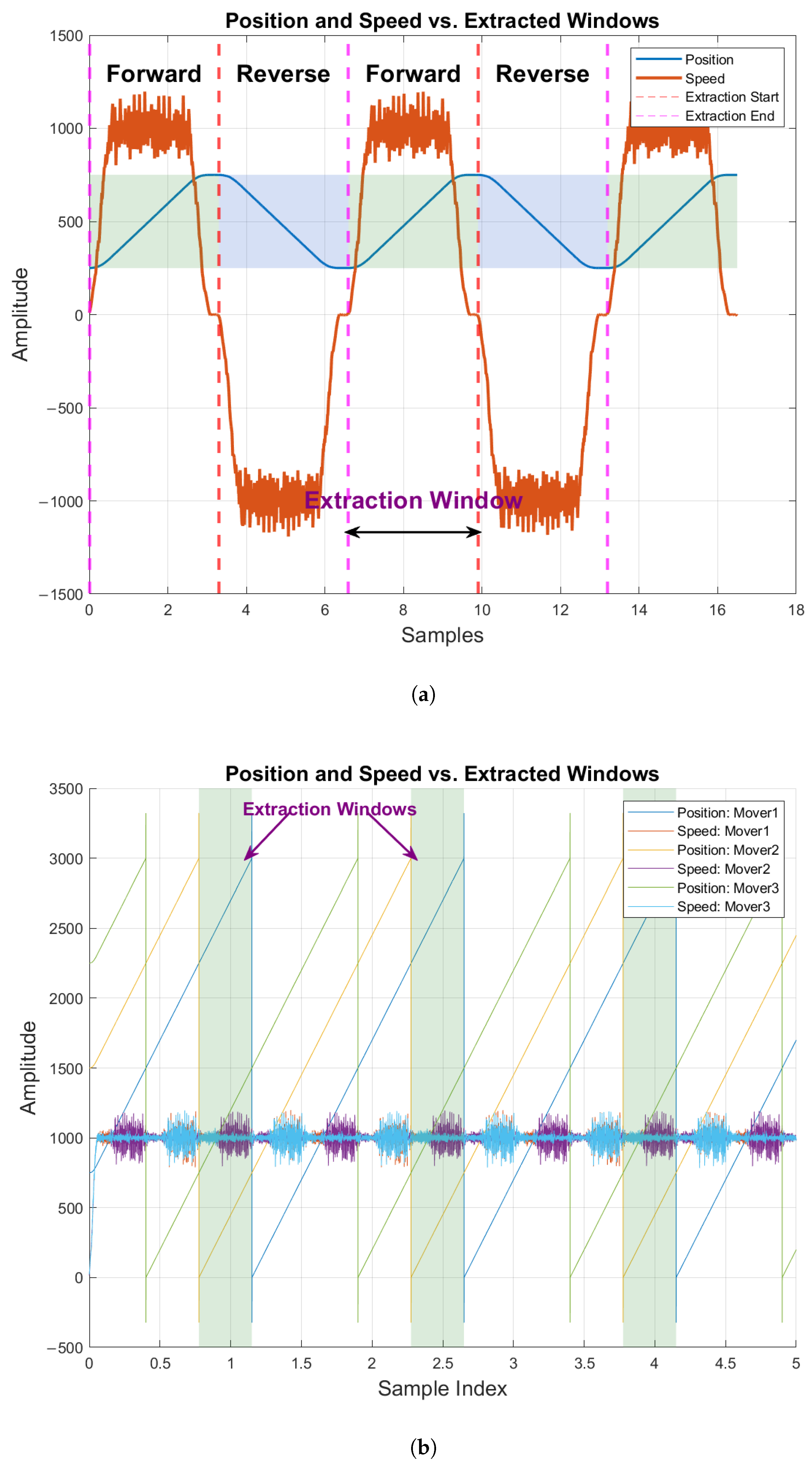
7. Preprocessing Methodology

Given the enormity of the data set, it is not feasible to include a detailed analysis for each experiment within the scope of this article. Instead, a selection of representative experiments is chosen for presentation in this section. These experiments illustrate the system’s behavior under varying experimental conditions and fault sizes.
The statistical features listed in Table 6 are extracted for each realization of the experiment, covering both fault-free and faulty conditions with varying fault sizes (see Table 7). For single-cart experiments, the data set includes five system variables: cart position, following error, actual velocity, velocity error, and set current of the cart. Additionally, nine vibration channels are recorded from five different accelerometers, resulting in 156 features per realization (excluding cart speed and velocity, as these channels were not considered for feature extraction). In the case of three-cart experiments, the number of vibration channels remains the same, but the system variables increase by a factor of three (one set per cart). This leads to an even higher-dimensional feature set compared to single-cart experiments. Given the large dimensionality of the data set for each experiment, visualizing the impact of individual features becomes challenging. To address this, we employ a feature ranking method prior to applying feature reduction techniques. Feature ranking helps identify the most significant features that contribute to the detection and characterization of faults, thereby reducing computational complexity and improving the interpretability of the results. This approach ensures that the most relevant features are retained for further analysis, enabling efficient and accurate fault diagnosis.

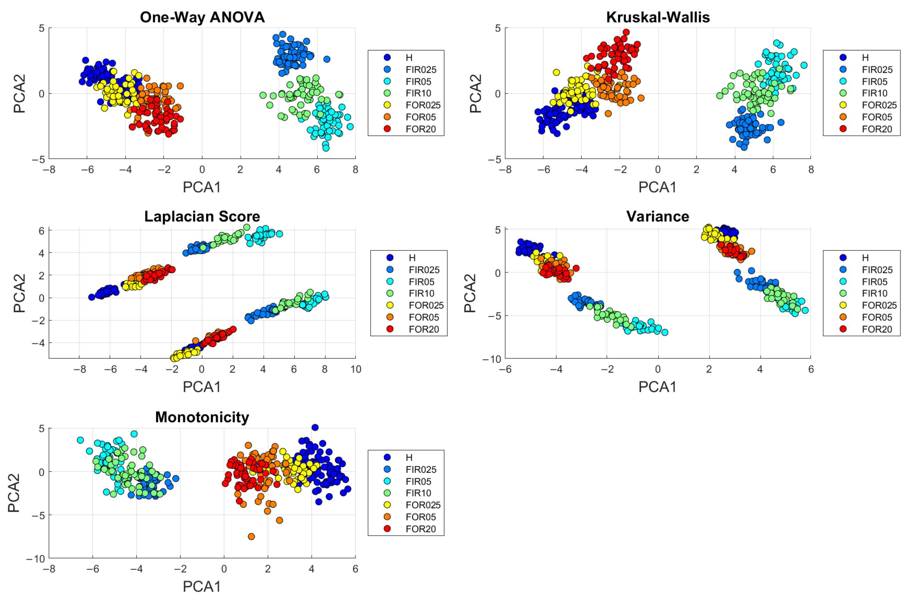
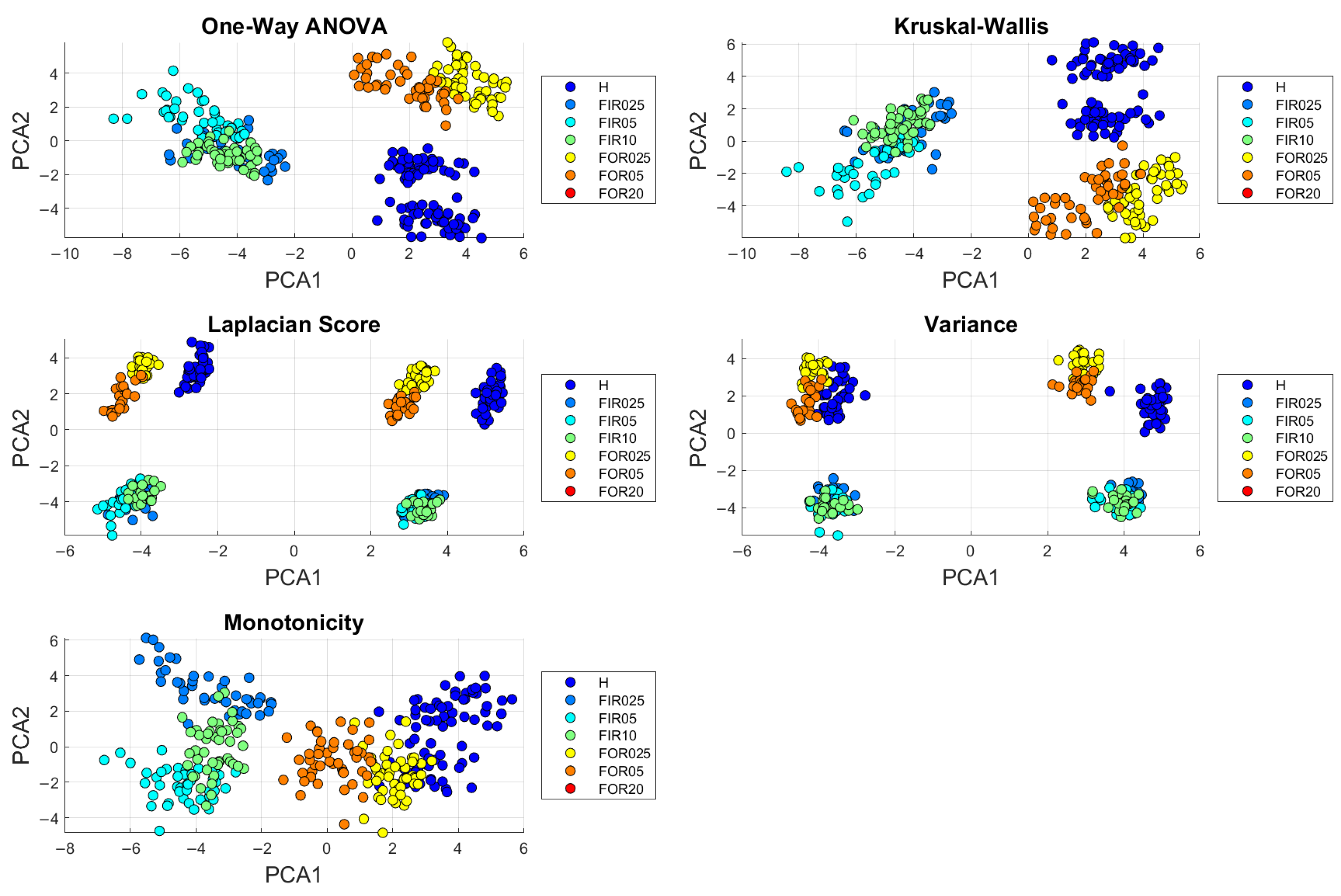
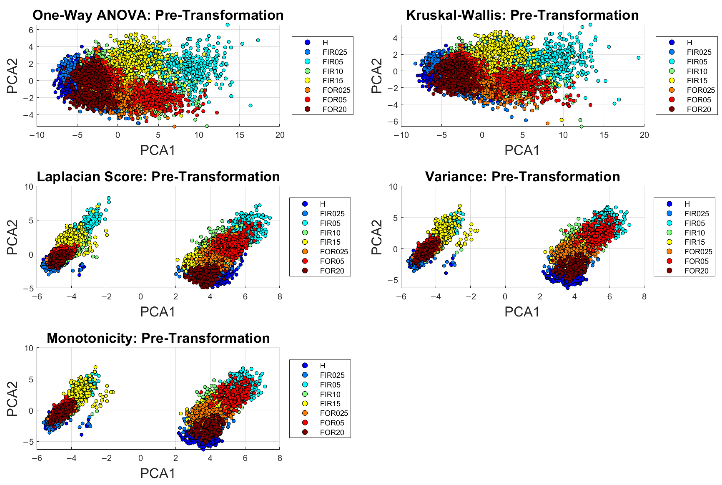
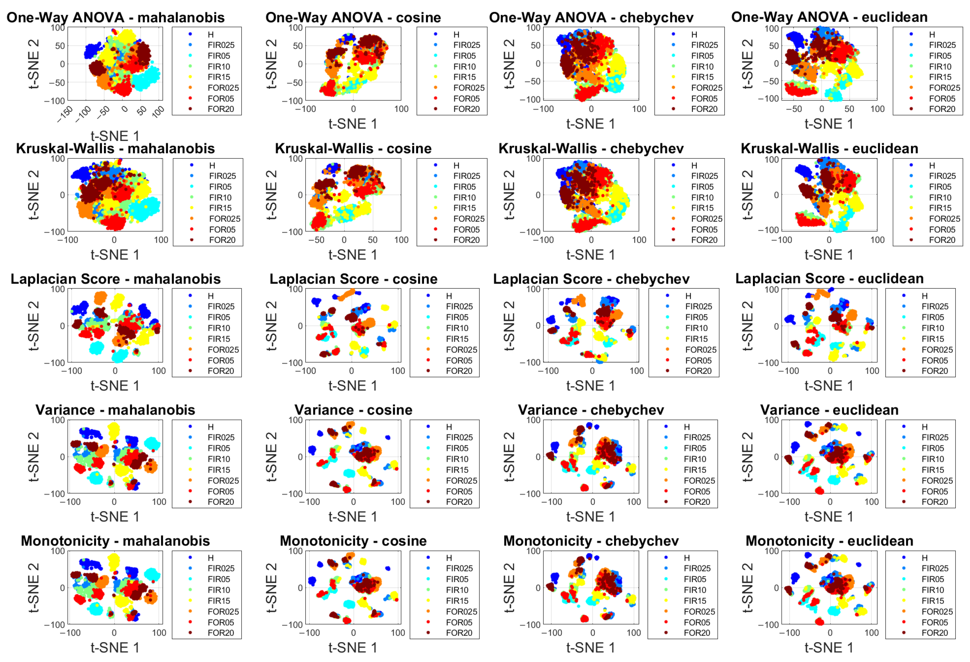
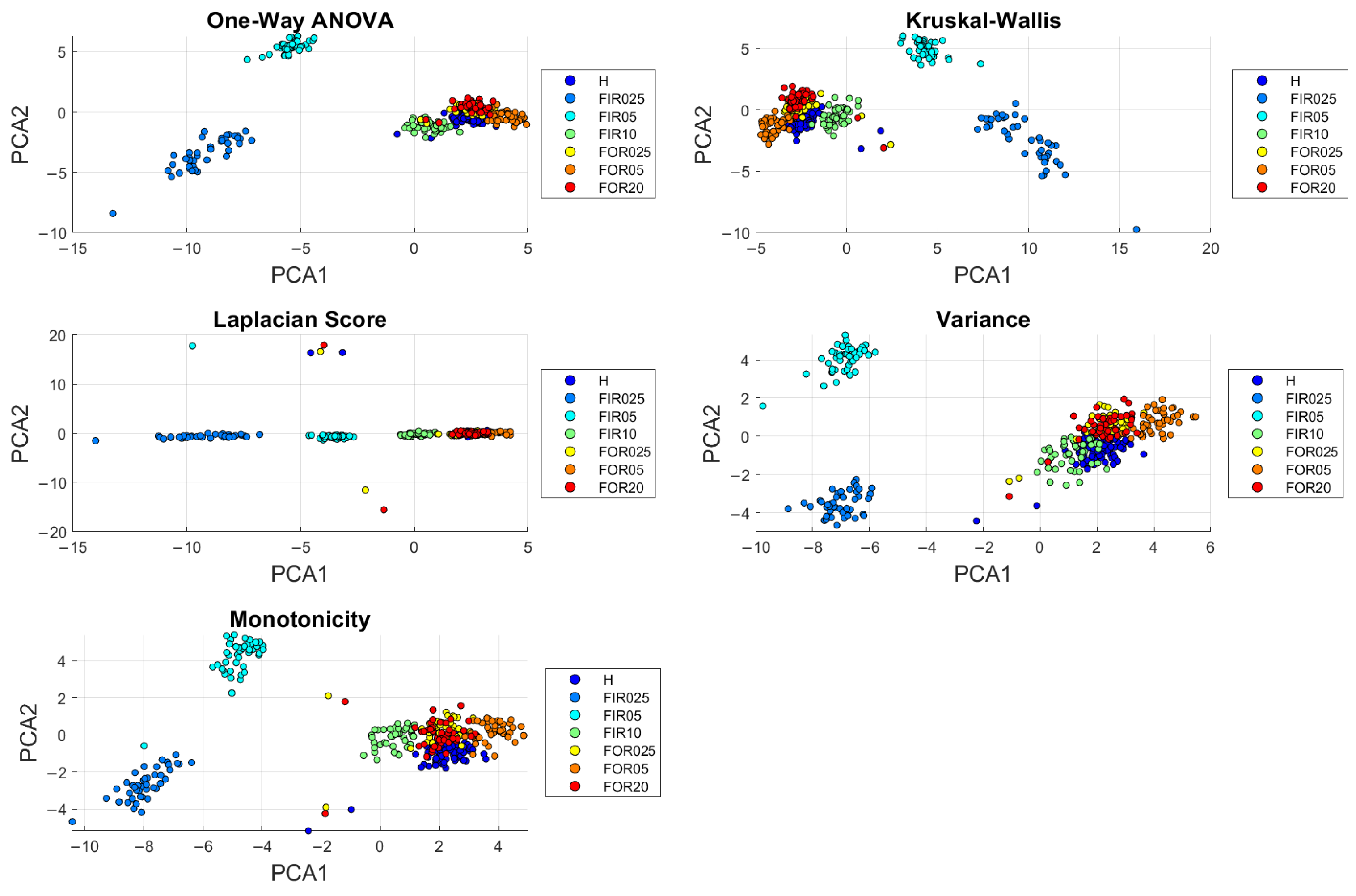
7.1. Feature Ranking Methods

Five feature-ranking methods, spanning both supervised and unsupervised approaches, were used to evaluate the importance of features to distinguish patterns and trends in the data set, while also reducing the computational cost for large data sets.

7.1.1. One-Way ANOVA

The One-Way Analysis of Variance (ANOVA) [42,43,44] is a statistical method used to identify significant differences between the means of two or more groups. In the context of feature ranking, ANOVA evaluates the relationship between a feature and the target variable, ranking features based on their ability to distinguish between different classes or groups. It assumes that the data within each group follow a normal distribution and that the variances are homogeneous between the groups. Mathematically, the test statistic for One-Way ANOVA is derived by partitioning the total variance of the data into variance between groups and variance within groups. For a feature X divided into k groups with n total samples, the statistic F is calculated as
F = Variance Between Groups Variance Within Groups = 1 k 1 i = 1 k n i ( X ¯ i X ¯ ) 2 1 n k i = 1 k j = 1 n i ( X i j X ¯ i ) 2
where X ¯ i is the mean of group i, X ¯ is the overall mean, n i is the number of samples in group i, k is the number of groups, and X i j is the j-th sample in group i. A higher F-statistic indicates that the feature effectively discriminates between groups, making it more relevant for classification or regression tasks. Features are ranked based on their corresponding F-statistics.

7.1.2. Kruskal–Wallis

The Kruskal–Wallis test [45,46] is a nonparametric method to test whether multiple independent samples originate from the same distribution. It is often used for feature ranking in data sets where the assumptions of parametric tests, such as normality and homogeneity of variances, may not hold. The test assesses whether there are statistically significant differences between the medians of groups for a given feature. Mathematically, for a feature X with k groups and n total observations, the Kruskal–Wallis test computes a test statistic H as
H = 12 n ( n + 1 ) i = 1 k R i 2 n i 3 ( n + 1 )
where n i is the number of observations in group i, R i is the mean rank of group i, and n is the total number of observations, given by n = i = 1 k n i . To compute H, the data are ranked in all groups, and these ranks are used to calculate the mean rank R i for each group. Under the null hypothesis that all groups come from the same distribution, the test statistic H approximately follows a chi-square ( χ 2 ) distribution with k 1 degrees of freedom, provided the sample size is large. A higher H statistic indicates that the feature effectively differentiates between groups, making it more relevant for the selection of features. The features are ranked according to their corresponding H statistics, with higher values indicating greater discriminatory power.

7.1.3. Laplacian Score

The Laplacian score [47] is a feature ranking method designed to evaluate the relevance of individual features based on their ability to preserve the intrinsic geometric structure of the data. Unlike methods that rely on labeled data, the Laplacian score is particularly effective for unsupervised learning, as it identifies features that maintain the locality information in the feature space. This makes it highly suitable for applications such as clustering, dimensionality reduction, and other tasks where preserving the data’s manifold structure is critical. Given a data set X R n × d , where n is the number of samples and d is the number of features, the method begins by constructing a similarity graph, which represents the relationships between the data points. For two data points x i and x j , the similarity W i j is computed using a Gaussian kernel, defined as
W i j = e x i x j 2 t , if x i N ( x j ) 0 , otherwise
where t is a scaling parameter, and N ( x i ) denotes the neighbors of x i . The diagonal degree matrix D is then calculated as D i i = j W i j , and the graph Laplacian matrix L is derived as L = D W . For a given feature F j , the Laplacian score is mathematically expressed as
S j = i , j ( x j , i x ¯ j ) ( x j , j x ¯ j ) W i j i ( x j , i x ¯ j ) 2 D i i
where x j , i is the value of the j-th feature for the i-th sample and x ¯ j is the mean of the j-th feature. Features with lower Laplacian scores preserve the locality of the data better and are ranked higher, making them more suitable for tasks such as clustering or dimensionality reduction.

7.1.4. Variance

The variance ranking method is a simple, yet effective approach for feature selection, primarily used in unsupervised learning scenarios. This method ranks features based on their variance under the assumption that features with higher variance contain more information and are more likely to be useful for distinguishing between data points. Variance is often used as a baseline method for feature selection because of its computational simplicity and intuitive nature. For a given data set X R n × d , where n is the number of samples and d is the number of features, the variance of the j-th feature F j is computed as
σ j 2 = 1 n i = 1 n ( x j , i μ j ) 2
where σ j 2 is the variance of the j-th feature, x j , i is the i-th sample of the j-th feature, and μ j is the mean of the j-th feature. The variance measures the dispersion of the data points around the mean of each feature. Features with higher variance are ranked higher, as they indicate greater variability and potential discriminatory power. Despite its simplicity, the variance ranking method has proven useful in a variety of applications, including dimensionality reduction, clustering, and preprocessing steps for more complex feature selection techniques. However, it assumes that high variance correlates with high relevance, which may not always hold true, especially in data sets with nonlinear relationships or noisy features.

7.1.5. Monotonicity

The monotonicity ranking method [48] evaluates the degree to which a feature changes consistently with respect to time or degradation progression, making it particularly useful for fault diagnosis and prognostics. Monotonicity can be computed using two approaches, depending on the specified method: the Signum method and Spearman’s rank correlation coefficient method. The Signum method measures monotonicity based on the consistency of directional changes (increases or decreases) in a feature over time. Mathematically, it is computed as
Monotonicity = 1 M j = 1 M 1 N j 1 k = 1 N j 1 sgn ( x j ( k + 1 ) x j ( k ) )
where x j represents the vector of measurements for a feature on the j-th system, M is the total number of systems monitored, N j is the number of measurements on the j-th system, and sgn ( · ) is the signum function. The method evaluates the fraction of consistent changes in the feature in all monitored systems, with higher values indicating stronger monotonicity. The Spearman rank method computes monotonicity based on the correlation between the ranks of the feature measurements and their corresponding time points. The formula for monotonicity using this method is
Monotonicity = 1 M j = 1 M corr ( rank ( x j ) , rank ( t j ) )
where x j represents the feature measurement vector on the j-th system, t j is the vector of time points corresponding to the measurements x j , M is the total number of systems monitored, and rank ( · ) denotes the ranking of elements in a vector.

7.2. Dimensionality Reduction

To address the high dimensionality of the data set, principal component analysis (PCA) and t-Distributed Stochastic Neighbor Embedding (t-SNE) were employed. These methods were chosen for their complementary strengths and widespread use in the literature. PCA is a well-established, computationally efficient method for linear dimensionality reduction. It is particularly effective for capturing global structures in high-dimensional data by identifying orthogonal directions of maximum variance [49,50]. Mathematically, PCA identifies orthogonal directions (principal components) by solving the eigenvalue decomposition of the covariance matrix of the data, thereby ensuring that the majority of the information is retained in a reduced set of dimensions. In the context of condition monitoring and fault diagnosis, PCA has proven invaluable for reducing noise and highlighting dominant patterns in the data [51]. On the other hand, t-SNE excels at preserving local structures and revealing clusters in high-dimensional data, making it highly suitable for visualizing complex relationships. t-SNE works by minimizing the Kullback–Leibler divergence between the high- and low-dimensional distributions of pairwise similarities. This approach is particularly effective for uncovering clusters, patterns, and relationships in complex data sets, making it well suited for this study [52,53]. Unlike PCA, t-SNE is capable of capturing nonlinear relationships, which are often critical for understanding fault patterns in mechanical systems [54]. By employing both PCA and t-SNE separately on the same data set, the unique strengths of each method are leveraged. PCA is utilized for efficient dimensionality reduction and noise reduction, enabling the identification of dominant patterns and global structures in the data. In contrast, t-SNE is applied for detailed visualization and cluster analysis, as it excels at preserving local structures and revealing nonlinear relationships. This dual approach allows for a comprehensive exploration of the data set from different perspectives, enhancing the ability to detect and diagnose faults robustly.

7.3. Speed Profiles

The speed profiles in these experiments exhibit non-synchronous behavior, particularly during the back-and-forth motion, where rapid speed changes occur because the cart decelerates as it stops before reversing direction and then accelerates as it changes direction until reaching the nominal speed again. This phenomenon becomes even more significant as the nominal speed increases. Figure 10 illustrates the speed profiles observed in various experimental configurations. Figure 10a shows the nominal speed profile of 1000 mm/s along the curved module of the system, representative of Experiment Type 2. In particular, this speed profile is consistent with other experiments involving back-and-forth movements, such as Experiment Types 1, 3, and 5. The primary distinction is that Experiment Type 5 features three movers, while Experiment Types 1, 2, and 3 involve a single mover. Figure 10b, on the other hand, represents the characteristic speed profiles of Experiment Types 4, 6, 7, and 8. In Experiment Type 4, a single mover continuously circulates along the track, whereas Experiment Types 6, 7, and 8 involve three movers executing similar continuous movements. The comparison across these profiles highlights the impact of varying the number of movers on the system’s dynamic behavior while maintaining consistency in movement patterns.

8. Data Visualization and Analysis

Results are provided for selected single-cart and three-cart experiments, focusing on varying defect sizes and IR fault orientations. The analysis explores key patterns in vibration signals and system variables, offering a comparative perspective in different experimental configurations. The original feature set, summarized in Table 4, was computed using all channels, including the following error, the velocity error, the set current for the movers, and the vibration channels, while excluding the position and speed of the cart. The exclusion of position and speed channels is based on the assumption that these are periodic and deterministic in nature. Consequently, while the reduced feature set excludes these deterministic channels, it does not solely represent vibration data, as it still incorporates other system-level variables. The defect labels corresponding to the experiments are detailed in Table 5, providing clarity on the types of faults and their respective sizes.

8.1. Single Cart Experiments

Scatter plots derived from Experiment Types 1 and 2 are presented to analyze the distribution of features in single-cart configurations. All plots correspond to a nominal cart speed of 1000 mm/s. For Experiment Type 1, only the PCA scatter plots are included, as the no-fault profile (or normal profile) can easily be distinguished from the abnormal profile in most fault categories using PCA alone. Figure 11 and Figure 12 illustrate that the PCA features corresponding to the healthy bearing state form a distinct cluster, clearly separated from the IR fault categories of all sizes. This distinction highlights the ability of PCA to reduce dimensionality while preserving the separability of the fault data. However, OR fault categories appear closer to the no-fault boundary, indicating overlapping feature distributions. Although this overlap suggests challenges in differentiating OR faults from the healthy state using PCA alone, further processing or advanced clustering techniques could help achieve a more compact and distinct representation for these fault classes. For Experiment Type 2 (Figure 13 and Figure 14), both PCA and t-SNE scatter plots are utilized to provide a more comprehensive visualization of the feature set. These plots represent experimental data for which the IR fault orientation information is unknown, as it was not recorded during the experiment. PCA applied to data sets ranked by one-way analysis of variance (ANOVA) and Kruskal–Wallis methods results in highly scattered features, with limited separability observed across all fault classes of the top bearing, including IR and OR faults. This outcome indicates the limitations of PCA when applied to these specific feature rankings. In contrast, PCA applied to data sets ranked by unsupervised methods—Laplacian Score, Variance, and Monotonicity—yields a bimodal distribution, suggesting a better representation of the underlying structure for these rankings. Similarly, the t-SNE reduced feature sets exhibit consistent bimodal distributions in nearly all distance metrics, including Mahalanobis, Cosine, Chebyshev, and Euclidean. These visualizations demonstrate that t-SNE effectively captures the underlying patterns in the feature set, revealing separability across fault categories, even under varying distance metrics. This underscores the significance of dimensionality reduction techniques, particularly for nonlinear methods such as t-SNE, in visualizing and analyzing high-dimensional data sets. However, the bimodal nature of the distributions in both PCA and t-SNE suggests that further processing is necessary to transform the feature distributions into Gaussian-like clusters. Such transformations could lead to more compact clustering and improved classification performance, which remains an area for future work.

8.2. Three Cart Experiments

For the three-mover experiments, the plots (Figure 15 and Figure 16) correspond to Experiment Type 8, conducted at a nominal cart speed of 1000 mm/s, with the relative distance between the movers set to 750 mm. The PCA-reduced feature set effectively distinguishes the normal profile from the FIR025 and FIR05 fault categories of the top bearing in all ranking methods, except the Laplacian score. In this case, the Laplacian Score performs poorly, failing to provide meaningful separability between the fault and no-fault states. This limitation may be attributed to the unsupervised nature of the Laplacian score, which prioritizes preserving the local data structure but may struggle to differentiate fault classes in complex data sets. Additionally, the FIR10 fault category appears closer to the OR fault classes in the PCA-reduced space, suggesting some overlap in the feature distributions. This overlap highlights the challenges in using PCA for separating fault types, particularly when the severity of the fault increases or when the faults share similarities in their vibration signatures. In contrast, t-SNE scatter plots offer superior fault separability for Experiment Type 8, providing a clearer visualization of the distinctions between normal and fault conditions. The t-SNE-reduced feature set demonstrates robust clustering across nearly all distance metrics, including Mahalanobis, Cosine, Chebyshev, and Euclidean. This improved separation underscores the strength of t-SNE in capturing nonlinear relationships within the high-dimensional feature set. In particular, t-SNE is able to resolve the overlap between FIR10 and OR fault classes observed in the PCA plots, providing a more distinct representation of the underlying feature space. These results highlight the importance of selecting appropriate dimensionality reduction techniques and distance metrics for effectively analyzing fault data in multicart configurations. Further work could focus on refining clustering techniques to enhance the compactness and separability of fault categories, particularly in cases where fault distributions exhibit overlap.

9. Conclusions

This study presents a comprehensive data set and analysis framework for the monitoring of the condition of independent cart systems, addressing the unique challenges posed by their complex configurations and motion dynamics. A key aspect of these systems is their scalability, where the addition of each cart increases the number of bearings by three, significantly amplifying the complexity of fault detection and localization. Furthermore, the unique translational and rotational dynamics of bearings, as they glide along the track, introduce challenges that differ fundamentally from the conventional rotary machinery. Through a systematic experimental campaign, data sets were collected under varying fault types, severities, and configurations, with a focus on single-cart and three-cart setups. The analysis employed classical statistical parameters, including mean, skewness, kurtosis, crest factor, and similar metrics, ensuring a straightforward yet effective approach for fault identification. Dimensionality reduction techniques such as PCA and t-SNE were also used to analyze the high-dimensional feature set, revealing critical insights into fault separability across different classification methods and experimental conditions. The results demonstrate the ability of PCA to distinguish between normal and faulty states, particularly for simpler configurations and smaller fault sizes. However, for complex scenarios, such as the three-cart experiments with overlapping fault distributions, t-SNE provided superior separability and visualization, especially when combined with robust distance metrics. These findings highlight the value of combining classical statistical features with modern dimensionality reduction techniques to provide simple but effective solutions for fault identification in industrial settings. The study also highlights the limitations of existing techniques in achieving compact clustering and fault localization, particularly for overlapping fault distributions and unsupervised ranking methods like the Laplacian score. Future work will focus on developing advanced clustering and transformation techniques to address these challenges, with a particular emphasis on resolving the issue of overlapping fault distributions. This includes enhancing fault discrimination between closely spaced fault conditions by leveraging adaptive feature transformations, improved metric learning, and advanced decision boundary refinement methods. These developments aim to improve the interpretability of fault signatures and ensure more reliable fault classification, even in complex multi-cart configurations.
The potential for failure prediction under broader experimental conditions is an important direction for future research. While the current study primarily focused on speed profiles of 1000 mm/s and 2000 mm/s, the developed methodology can be extended to a wider range of operating conditions. Future work could explore varying load conditions, acceleration profiles, and adaptive speed scenarios, which are more representative of real-world industrial settings. Additionally, incorporating environmental factors such as temperature variations, lubrication conditions, and external disturbances could further enhance the generalizability of the proposed approach. Furthermore, the inclusion of detailed experimental data in an open-access repository ensures that this work serves as a valuable resource for the research community, fostering innovation in predictive maintenance and machine health monitoring for modern industrial transport systems. By making the data set openly accessible, this study provides a foundation for further research in predictive maintenance and condition monitoring, not only for independent cart systems but also for other industrial applications.

Author Contributions

Conceptualization, A.J., M.C., G.D., D.B., J.C.C.M., M.S. and R.R.; Methodology, A.J., L.C. and J.C.C.M.; Software, A.J., G.D., L.C. and J.C.C.M.; Validation, A.J. and G.D.; Resources, D.B. and L.C.; Data curation, A.J. and L.C.; Writing—original draft, A.J.; Writing—review & editing, M.C., G.D., J.C.C.M., M.S. and R.R.; Supervision, M.C. and D.B. All authors have read and agreed to the published version of the manuscript.

Funding

This research was funded by the European Commission for its support of the Marie Sklodowska Curie Program through the H2020 ETN MOIRA project (GA 955681).

Institutional Review Board Statement

Not applicable.

Informed Consent Statement

Not applicable.

Data Availability Statement

The data presented in this study are openly available in Zenodo at the links provided in the references [37,38,39,40,41].

Acknowledgments

The authors gratefully acknowledge the European Commission for its support of the Marie Sklodowska Curie Program through the H2020 ETN MOIRA project (GA 955681). The authors also thank Giovanni Paladini at Beckhoff Italy for his support in troubleshooting the hardware and motor firmware-related aspects of the experimental setup.

Conflicts of Interest

Authors Davide Borghi, Luca Capelli and Jacopo Cavalaglio Camargo Molano were employed by the company Tetra Pak Packaging Solutions. The remaining authors declare that the research was conducted in the absence of any commercial or financial relationships that could be construed as a potential conflict of interest.

Appendix A

Appendix A.1. Data Variables Naming Conventions

Appendix A.1.1. System Variables

  • For single-cart experiments, variables are not suffixed with cart numbers.
  • For three-cart experiments, the variables are suffixed with _M1, _M2, and _M3 to denote individual carts.

Appendix A.1.2. Vibration Channels

Mono-Axial Accelerometers 

  • mono_PCB_Top: PCB-manufactured accelerometer mounted on the top section of the guide rail, positioned halfway along the track.
  • mono_ifm_Top: ifm-manufactured accelerometer, also near the top section of the guide rail on an aluminum rod, positioned halfway along the track.
  • mono_PCB_Bottom: PCB-manufactured accelerometer mounted on the bottom section of the guide rail, positioned halfway along the track.

Tri-Axial Accelerometers 

  • Sensors capturing vibrations in the X, Y, and Z directions, mounted on the left and right sides of the guide.
Table A1. Data variable classification and naming convention by experiment type.
CategoryVariable TypeSingle-Cart ExperimentsThree-Cart Experiments
System VariablesPositionActHwPosActHwPos_M1
ActHwPos_M2
ActHwPos_M3
Following ErrorActFollowingErrorActFollowingError_M1
ActFollowingError_M2
ActFollowingError_M3
VelocityActVeloActVelo_M1
ActVelo_M2
ActVelo_M3
Velocity ErrorActVeloErrorActVeloError_M1
ActVeloError_M2
ActVeloError_M3
Set CurrentSetCurrSetCurr_M1
SetCurr_M2
SetCurr_M3
Vibration ChannelsMono-Axialmono_PCB_Top
mono_ifm_Top
mono_PCB_Bottom
mono_PCB_Top
mono_ifm_Top
mono_PCB_Bottom
Tri-AxialX_Guide_Left
Y_Guide_Left
Z_Guide_Left
X_Guide_Right
Y_Guide_Right
Z_Guide_Right
X_Guide_Left
Y_Guide_Left
Z_Guide_Left
X_Guide_Right
Y_Guide_Right
Z_Guide_Right

Appendix A.2. File Naming Conventions for Experimental Data

The file naming convention systematically encodes the details of each experiment, making it easy to identify the type of experiment, the fault conditions, the speed profiles and other critical parameters. The file names are classified into two main categories: single-mover experiments (Experiment Types 1–4) and three-cart experiments (Experiment Types 5–8). The convention follows a structured format:

Appendix A.2.1. Experiment Type 1–4

<Fault Condition>_<Experiment Category>_<Experiment Description>_<Speed>_ <Fault Details>_<Fault Location>_<Trial Number>

Appendix A.2.2. Experiment Type 5–8

<Fault Condition>_<Experiment Category>_<Experiment Description>_<Separation Details>_<Speed>_ <Fault Details>_<Fault Location>_<Trial Number>

Appendix A.3. Description of File Names

Each element of the file names conveys specific information about the corresponding experiment, such as the type of experiment, fault conditions, and speed profiles. The meaning of each element is systematically encoded and can be interpreted as described below.

Fault Condition

  • H: No Fault (Healthy).
  • F: Bearing Fault.

Experiment Category

  • SingleMover: Single-cart experiments.
  • 3Movers: Three-cart experiments.

Experiment Description

  • StraightTop: Straight path back-and-forth movement along the upper section of the guide rail.
  • Curved: Back-and-forth movement limited to the curved module only.
  • CompleteRotation: Circular movement along the track.

Separation Details

  • 150mmSeparation: The relative distance between two carts is150 mm.
  • 250mmSeparation: The relative distance between two carts is 250 mm.
  • 500mmSeparation: The relative distance between two carts is 500 mm.
  • 750mmSeparation: The relative distance between two carts is 750 mm.

Speed

  • 1000: Nominal cart speed profile of 1000 mm/s.
  • 2000: Nominal cart speed profile of 2000 mm/s.

Fault Details

  • Fault Type: IR (Inner Race), OR (Outer Race).
  • Fault Severity: Fault width, 025 (0.25 mm), 05 (0.5 mm), 10 (1.0 mm), 15 (1.5 mm) and 20 (2.0 mm).

Fault Location

  • Top: Top bearing.
  • Bottom: Bottom bearing.

Trial Number

  • Denotes the trial or realization number for the specific experiment (e.g., Real1).

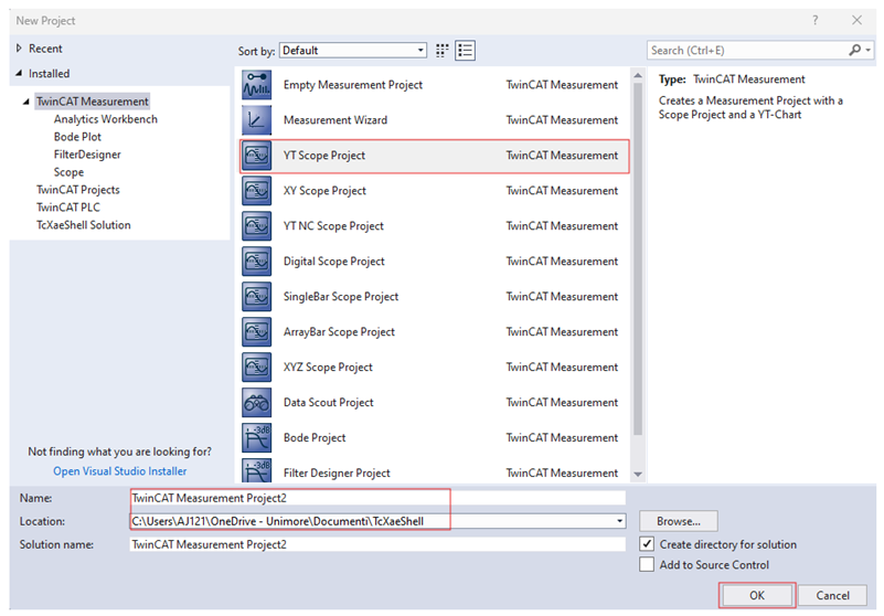
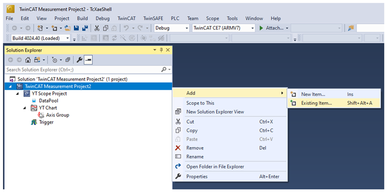
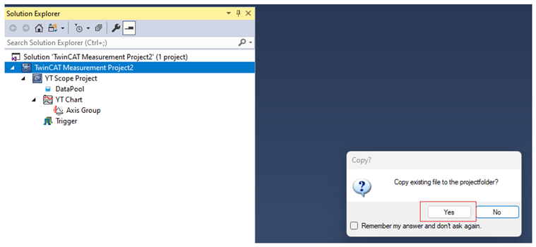
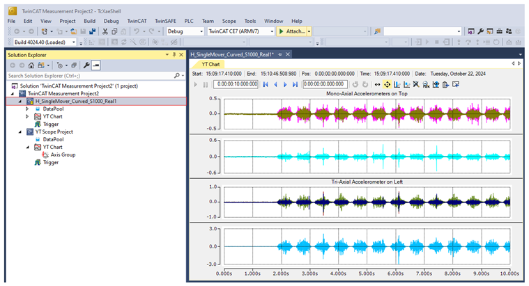
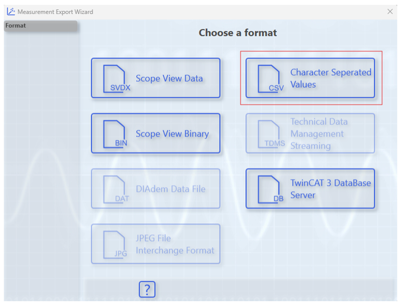
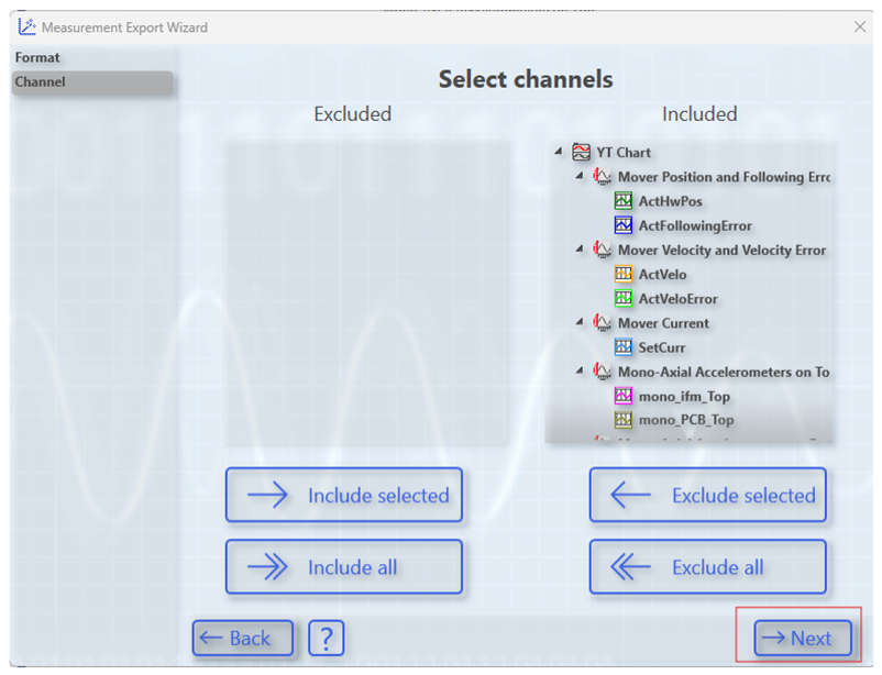
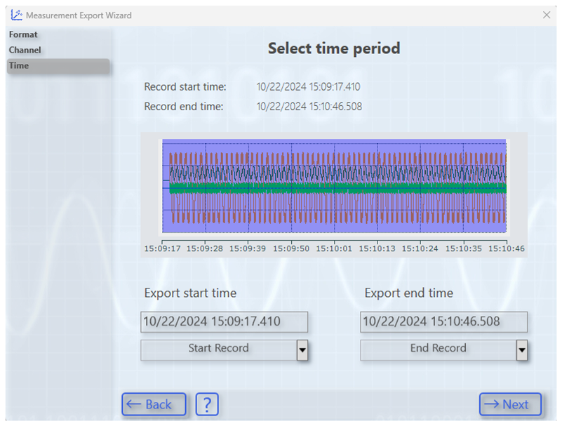
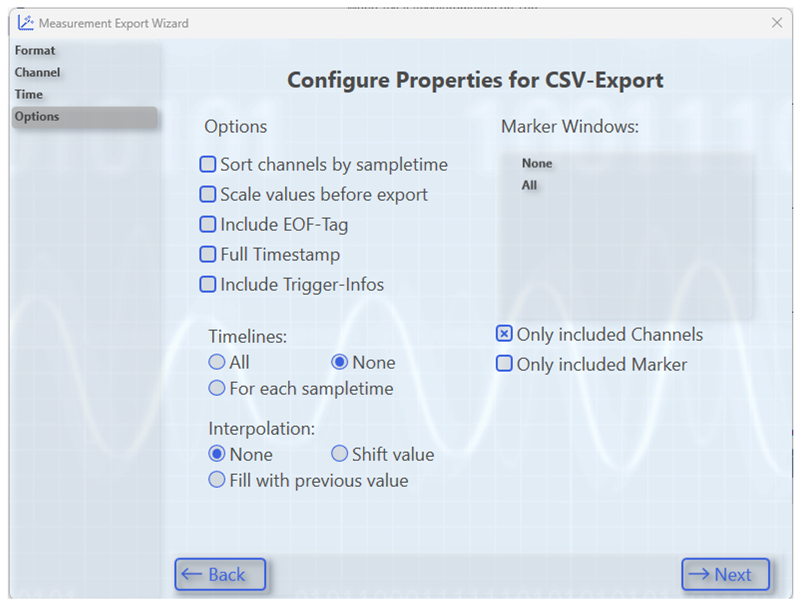
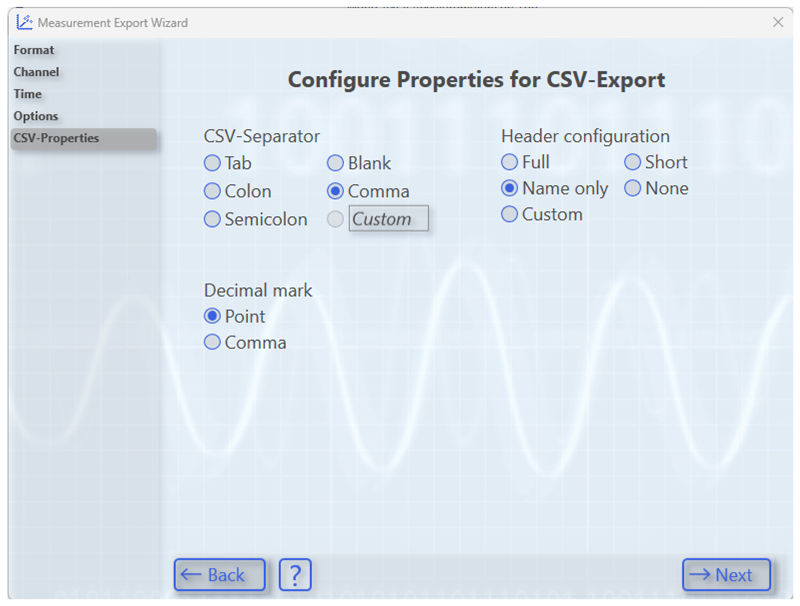
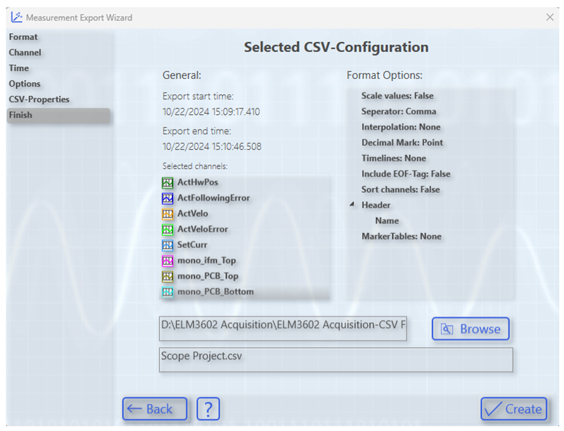
Appendix A.4. Creating and Exporting a YT Scope Project in TwinCAT XAE Shell

TwinCAT, developed and licensed by Beckhoff, stands for Windows Control and Automation Technology. It is advanced automation software that transforms almost any PC-based system into a real-time control platform, supporting multiple runtime PLC, NC, CNC, and robotics systems. The latest version, TwinCAT 3, was utilized to record the data set in this study. TwinCAT 3 is freely available for download from the Beckhoff website. Although it requires a weekly renewal of the license, this process is straightforward and cost-free. Users simply enter an automatically generated code into a dialog box to extend the license.
Step 1—Create New Measurement Project: Open the TwinCAT XAE shell and select New Measurement Project to begin.
Applsci 15 03691 i001
Step 2—Name and Save the Project: Choose the type of measurement project, which in this case is the YT Scope Project. Provide a name for the project and specify the save directory.
Applsci 15 03691 i002
Step 3—Add Existing Files to the Project: After creating the project, add existing “.svdx” files from the save directory as shown in the accompanying image. Multiple files can be added simultaneously. For this example, we load a single file.
Applsci 15 03691 i003
Step 4—Copy Files to the Project Directory: Choose whether to copy the selected files to the project directory. It is recommended to copy them for easier management. Once the files are converted to the desired format, you can delete the original “.svdx” files to free up memory.
Applsci 15 03691 i004
Step 5—Visualize the YT Scope Project: To visualize the data channels, left-click on the file “.svdx” in the project tree.
Applsci 15 03691 i005
Step 6—Export Project: To export the project in the desired format, go to the Scope tab in the options bar at the top and select Scope –> Export.
Applsci 15 03691 i006
Step 7—Choose Format: A new window will appear, guiding you through the format conversion steps. Start by selecting the desired data format. In this example, we select the Character Separated Values (CSV) format.
Applsci 15 03691 i007
Step 8—Select Channels: After selecting the format, choose the data channels to be exported and proceed by clicking Next.
Applsci 15 03691 i008
Step 9—Select Time Duration: Specify the time range for data conversion. For this example, we select End of Record.
Applsci 15 03691 i009
Step 10—Configure CSV Options: Choose the metadata settings for export. In this example, we select Only Included Channels under Marker Windows, None for Timelines, and None for Interpolation.
Applsci 15 03691 i010
Step 11—Configure CSV Properties: Set CSV-specific properties, such as the Separator and Decimal Mark, to suit your preferences.
Applsci 15 03691 i011
Step 12—Name and Save File: Finally, provide a name for the converted file and choose a save directory to complete the export process.
Applsci 15 03691 i012

References

  1. Beckhoff Automation. Extended Transport Systems (XTS). Available online: https://www.beckhoff.com/en-en/products/motion/xts-linear-product-transport/?msclkid=fd69f89dec35190c45d89f054681eef2 (accessed on 20 January 2025).
  2. Rockwell Automation. Independent Cart Technology. Available online: https://www.rockwellautomation.com/en-us/products/hardware/independent-cart-technology.html (accessed on 20 January 2025).
  3. Jabbar, A.; D’Elia, G.; Cocconcelli, M. Experimental Setup for Non-stationary Condition Monitoring of Independent Cart Systems. In International Congress and Workshop on Industrial AI and eMaintenance; Kumar, U., Karim, R., Galar, D., Kour, R., Eds.; Springer Nature: Cham, Switzerland, 2024; pp. 517–530. [Google Scholar] [CrossRef]
  4. Jabbar, A.; Cocconcelli, M.; d’Elia, G.; Strozzi, M.; Rubini, R. Results on Experimental Data Analysis of Independent Cart Systems in Non-Stationary Conditions. In Surveillance, Vibrations, Shock and Noise; Institut Supérieur de l’Aéronautique et de l’Espace [ISAE-SUPAERO]: Toulouse, France, 2023; hal-04165905. [Google Scholar]
  5. Xu, J.; Zhao, L.; Ren, Y.; Li, Z.; Abbas, Z.; Zhang, L.; Islam, M.S. LightYOLO: Lightweight model based on YOLOv8n for defect detection of ultrasonically welded wire terminations. Eng. Sci. Technol. Int. J. 2024, 60, 101896. [Google Scholar] [CrossRef]
  6. Lazović, T.; Marinković, A.; Atanasovska, I.; Sedak, M.; Stojanović, B. From Innovation to Standardization—A Century of Rolling Bearing Life Formula. Machines 2024, 12, 444. [Google Scholar] [CrossRef]
  7. Pastukhov, A.; Timashov, E. Procedure for Simulation of Stable Thermal Conductivity of Bearing Assemblies. Adv. Eng. Lett. 2023, 2, 58–63. [Google Scholar] [CrossRef]
  8. Kamat, P.; Kumar, S.; Sugandhi, R. Vibration-based anomaly pattern mining for remaining useful life (RUL) prediction in bearings. J. Braz. Soc. Mech. Sci. Eng. 2024, 46, 290. [Google Scholar] [CrossRef]
  9. Wu, Y.; Zhao, R.; Jin, W.; Deng, L.; He, T.; Ma, S. Rolling Bearing Fault Diagnosis Using a Deep Convolutional Autoencoding Network and Improved Gustafson-Kessel Clustering. Shock Vib. 2020, 2020, 8846589. [Google Scholar] [CrossRef]
  10. Barcelos, A.S.; Cardoso, A.J.M. Current-based bearing fault diagnosis using deep learning algorithms. Energies 2021, 14, 2509. [Google Scholar] [CrossRef]
  11. Ma, J.; Zhang, H.; Yang, S.; Jiang, J.; Li, G. An Improved Robust Sparse Convex Clustering. Tsinghua Sci. Technol. 2023, 28, 989–998. [Google Scholar] [CrossRef]
  12. Chen, J.; Wang, G.; Lv, J.; He, Z.; Yang, T.; Tang, C. Open-Set Classification for Signal Diagnosis of Machinery Sensor in Industrial Environment. IEEE Trans. Ind. Inform. 2023, 19, 2574–2584. [Google Scholar] [CrossRef]
  13. He, D.; Zhao, J.; Jin, Z.; Huang, C.; Zhang, F.; Wu, J. Prediction of bearing remaining useful life based on a two-stage updated digital twin. Adv. Eng. Inform. 2025, 65, 103123. [Google Scholar] [CrossRef]
  14. Sun, Y.; Tao, H.; Stojanovic, V. Pseudo-label guided dual classifier domain adversarial network for unsupervised cross-domain fault diagnosis with small samples. Adv. Eng. Inform. 2025, 64, 102986. [Google Scholar] [CrossRef]
  15. Chang, Q.; Fang, C.; Zhou, W.; Meng, X. A multi-order moment matching-based unsupervised domain adaptation with application to cross-working condition fault diagnosis of rolling bearings. Struct. Health Monit. 2024. [Google Scholar] [CrossRef]
  16. Xu, H.; Peng, X.; Wang, J.; Liu, J.; He, C. Adaptive graph-guided joint soft clustering and distribution alignment for cross-load and cross-device rotating machinery fault transfer diagnosis. Meas. Sci. Technol. 2024, 35, 045009. [Google Scholar] [CrossRef]
  17. Wang, G.; Huang, J.; Zhang, F. Ensemble clustering-based fault diagnosis method incorporating traditional and deep representation features. Meas. Sci. Technol. 2021, 32, 095110. [Google Scholar] [CrossRef]
  18. Wu, J.; Lin, M.; Lv, Y.; Cheng, Y. Intelligent fault diagnosis of rolling bearings based on clustering algorithm of fast search and find of density peaks. Qual. Eng. 2023, 35, 399–412. [Google Scholar] [CrossRef]
  19. Lu, Y.; Wang, Z.; Zhu, D.; Gao, Q.; Sun, D. Bearing Fault Diagnosis Based on Clustering and Sparse Representation in Frequency Domain. IEEE Trans. Instrum. Meas. 2021, 70, 3513914. [Google Scholar] [CrossRef]
  20. Xu, F.; Fang, Y.J.; Wang, D.; Liang, J.Q.; Tsui, K.L. Combining DBN and FCM for Fault Diagnosis of Roller Element Bearings without Using Data Labels. Shock Vib. 2018, 2018, 3059230. [Google Scholar] [CrossRef]
  21. Xu, F.; Tse, P.W. Combined deep belief network in deep learning with affinity propagation clustering algorithm for roller bearings fault diagnosis without data label. JVC/J. Vib. Control 2019, 25, 473–482. [Google Scholar] [CrossRef]
  22. Zhao, X.; Jia, M. A novel deep fuzzy clustering neural network model and its application in rolling bearing fault recognition. Meas. Sci. Technol. 2018, 29, 125005. [Google Scholar] [CrossRef]
  23. Wen, H.; Guo, W.; Li, X. A novel deep clustering network using multi-representation autoencoder and adversarial learning for large cross-domain fault diagnosis of rolling bearings. Expert Syst. Appl. 2023, 225, 120066. [Google Scholar] [CrossRef]
  24. Wei, J.; Huang, H.; Yao, L.; Hu, Y.; Fan, Q.; Huang, D. New imbalanced fault diagnosis framework based on Cluster-MWMOTE and MFO-optimized LS-SVM using limited and complex bearing data. Eng. Appl. Artif. Intell. 2020, 96, 103966. [Google Scholar] [CrossRef]
  25. Hang, Q.; Yang, J.; Xing, L. Diagnosis of rolling bearing based on classification for high dimensional unbalanced data. IEEE Access 2019, 7, 79159–79172. [Google Scholar] [CrossRef]
  26. Mamun, A.A.; Bappy, M.M.; Mudiyanselage, A.S.; Li, J.; Jiang, Z.; Tian, Z.; Fuller, S.; Falls, T.C.; Bian, L.; Tian, W. Multi-channel sensor fusion for real-time bearing fault diagnosis by frequency-domain multilinear principal component analysis. Int. J. Adv. Manuf. Technol. 2023, 124, 1321–1334. [Google Scholar] [CrossRef]
  27. Wang, C.; Nie, J.; Yin, P.; Xu, J.; Yu, S.; Ding, X. Unknown fault detection of rolling bearings guided by global–local feature coupling. Mech. Syst. Signal Process. 2024, 213, 111331. [Google Scholar] [CrossRef]
  28. Hu, B. Bearing data set. IEEE Dataport 2023. [Google Scholar] [CrossRef]
  29. Lee, J.; Qiu, H.; Yu, G.; Lin, J.; Rexnord Technical Services. IMS, University of Cincinnati. “Bearing Data Set”; NASA Prognostics Data Repository, NASA Ames Research Center: Moffett Field, CA, USA, 2007.
  30. Daga, A.P.; Fasana, A.; Marchesiello, S.; Garibaldi, L. The Politecnico di Torino rolling bearing test rig: Description and analysis of open access data. Mech. Syst. Signal Process. 2019, 120, 252–273. [Google Scholar] [CrossRef]
  31. Case Western Reserve University CWRU) Bearing Data Center. Available online: https://engineering.case.edu/bearingdatacenter (accessed on 20 January 2025).
  32. Wang, B.; Lei, Y.; Li, N.; Li, N. A Hybrid Prognostics Approach for Estimating Remaining Useful Life of Rolling Element Bearings. IEEE Trans. Reliab. 2020, 69, 401–412. [Google Scholar] [CrossRef]
  33. Shao, S.; McAleer, S.; Yan, R.; Baldi, P. Highly Accurate Machine Fault Diagnosis Using Deep Transfer Learning. IEEE Trans. Ind. Inform. 2018, 15, 2446–2455. [Google Scholar]
  34. Nectoux, P.; Gouriveau, R.; Medjaher, K.; Ramasso, E.; Morello, B.; Zerhouni, N.; Varnier, C. PRONOSTIA: An Experimental Platform for Bearings Accelerated Life Test. In Proceedings of the IEEE International Conference on Prognostics and Health Management, Denver, CO, USA, 18–21 June 2012. [Google Scholar]
  35. Hepco Motion. GFX- Guidance System for Backhoff XTS Linear Transport System. Available online: https://www.hepcomotion.com/product/driven-track-systems/gfx-guidance-system-for-beckhoff-xts-linear-transport-system (accessed on 20 January 2025).
  36. Jabbar, A.; Mazzonetto, M.; Orazi, L.; Cocconcelli, M. Ultrafast laser damaging of ball bearings for the condition monitoring of a fleet of linear motors. In Proceedings of the PHM Society European Conference 2024, Prague, Czech Republic, 3–5 July 2024; Volume 8, p. 10. [Google Scholar] [CrossRef]
  37. MOIRA-UNIMORE Bearing Data Set for Independent Cart Systems—Experiment Type 1 and 2. Available online: https://zenodo.org/records/14753683 (accessed on 29 January 2025).
  38. MOIRA-UNIMORE Bearing Data Set for Independent Cart Systems—Experiment Type 3 and 4. Available online: https://zenodo.org/records/14755761 (accessed on 29 January 2025).
  39. MOIRA-UNIMORE Bearing Data Set for Independent Cart Systems—Experiment Type 5 and 6. Available online: https://zenodo.org/records/14761243 (accessed on 29 January 2025).
  40. MOIRA-UNIMORE Bearing Data Set for Independent Cart Systems—Experiment Type 7. Available online: https://zenodo.org/records/14764717 (accessed on 29 January 2025).
  41. MOIRA-UNIMORE Bearing Data Set for Independent Cart Systems—Experiment Type 8. Available online: https://zenodo.org/records/14765815 (accessed on 29 January 2025).
  42. Fisher, R.A. Statistical Methods for Research Workers; Oliver and Boyd: Edinburgh, UK, 1925. [Google Scholar]
  43. Montgomery, D.C. Design and Analysis of Experiments; John Wiley & Sons: Hoboken, NJ, USA, 2017. [Google Scholar]
  44. Neter, J.; Kutner, M.H.; Nachtsheim, C.J.; Wasserman, W. Applied Linear Statistical Models, 4th ed.; Irwin Press: Chicago, IL, USA, 1996. [Google Scholar]
  45. Kruskal, W.H.; Wallis, W.A. Use of ranks in one-criterion variance analysis. J. Am. Stat. Assoc. 1952, 47, 583–621. [Google Scholar] [CrossRef]
  46. Sheskin, D.J. Handbook of Parametric and Nonparametric Statistical Procedures; Chapman & Hall/CRC: Boca Raton, FL, USA, 2003. [Google Scholar]
  47. He, X.; Cai, D.; Niyogi, P. Laplacian Score for Feature Selection. Adv. Neural Inf. Process. Syst. 2005, 18, 507–514. [Google Scholar]
  48. Coble, J.; Hines, J.W. Identifying Optimal Prognostic Parameters from Data: A Genetic Algorithms Approach. In Proceedings of the Annual Conference of the Prognostics and Health Management Society, San Diego, CA, USA, 28 September–1 October 2009. [Google Scholar]
  49. Pořízka, P.; Klus, J.; Képeš, E.; Prochazka, D.; Hahn, D.W.; Kaiser, J. On the utilization of principal component analysis in laser-induced breakdown spectroscopy data analysis, a review. Spectrochim. Acta Part At. Spectrosc. 2018, 148, 65–82. [Google Scholar] [CrossRef]
  50. Jolliffe, I.T.; Cadima, J. Principal component analysis: A review and recent developments. Phil. Trans. R. Soc. A 2016, 374, 20150202. [Google Scholar] [CrossRef] [PubMed]
  51. Kitao, A. Principal Component Analysis and Related Methods for Investigating the Dynamics of Biological Macromolecules. J 2022, 5, 298–317. [Google Scholar] [CrossRef]
  52. Jung, S.; Dagobert, T.; Morel, J.; Facciolo, G. A Review of t-SNE. Image Process. Line 2024, 14, 250–270. [Google Scholar] [CrossRef]
  53. van der Maaten, L.; Hinton, G. Visualizing Data using t-SNE. J. Mach. Learn. Res. 2008, 9, 2579–2605. [Google Scholar]
  54. Gove, R.; Cadalzo, L.; Leiby, N.; Singer, J.M.; Zaitzeff, A. New guidance for using t-SNE: Alternative defaults, hyperparameter selection automation, and comparative evaluation. Vis. Inform. 2022, 6, 87–97. [Google Scholar] [CrossRef]
Figure 1. The experimental independent cart system, illustrating all components, including the linear motors, carts, bearings, and guide rail.
Applsci 15 03691 g001
Figure 2. The experimental independent cart system, illustrating its modular nature.
Applsci 15 03691 g002
Figure 3. Picosecond laser beam profile.
Applsci 15 03691 g003
Figure 4. A schematic of the laser ablation system.
Applsci 15 03691 g004
Figure 5. Positioning of bearings on an ad hoc support. The operating principle of the multi-altitude approach for progressive focusing is explained in the enlarged image.
Applsci 15 03691 g005
Figure 6. Microscopic view of bearing faults: (a) Incipient version IR fault of bottom bearing, (b) Incipient version OR fault of bottom bearing, (c) Lase version 0.5 OR fault of top bearing, (d) Lase version 1.0 OR fault of bottom bearing, (e) Lase version 0.5 IR fault of bottom bearing.
Applsci 15 03691 g006
Figure 7. Experimental configuration detailing the number of carts used in each experiment, the relative distances between carts, sensor placements, and the specified movement patterns of the carts.
Applsci 15 03691 g007
Figure 8. High-level data acquisition strategy illustrating single-mover and three-mover experiments, including fault size details and speed profiles.
Applsci 15 03691 g008
Figure 9. Bearing assembly highlighting the inner race fault and its four angular orientations (0°, 90°, 180°, 270°) used for experimental fault positioning.
Applsci 15 03691 g009
Figure 10. Speed vs. Position profiles of the independent cart system with highlighted extraction windows, illustrating variations across different experimental configurations. (a) Single-cart experiment showing the velocity-position relationship for one cart. (b) Multi-cart experiment involving three carts, demonstrating the combined effect of multiple carts on the motion profile. Position is measured in millimeters (mm), and speed in millimeters per second (mm/s).
Applsci 15 03691 g010
Figure 11. PCA representation of the ranked feature set from Experiment Type 1, illustrating the IR and OR faults of the top bearing, with the IR fault oriented at 3 O’Clock.
Applsci 15 03691 g011
Figure 12. PCA representation of the ranked feature set from Experiment Type 1, illustrating the IR and OR faults of the bottom bearing, with the IR fault oriented at 3 O’Clock.
Applsci 15 03691 g012
Figure 13. PCA representation of the ranked feature set from Experiment Type 2, illustrating the IR and OR faults of the top bearing, without consideration of the IR fault orientation.
Applsci 15 03691 g013
Figure 14. t-SNE representation of the ranked feature set from Experiment Type 2, illustrating the IR and OR faults of the top bearing, without consideration of the IR fault orientation.
Applsci 15 03691 g014
Figure 15. PCA representation of the ranked feature set from Experiment Type 8, illustrating the IR and OR faults of the top bearing, with the IR fault oriented at 3 O’Clock. The features are computed for each complete cycle of the M1 mover.
Applsci 15 03691 g015
Figure 16. t-SNE representation of the ranked feature set from Experiment Type 8, illustrating the IR and OR faults of the top bearing, with the IR fault oriented at 3 O’Clock. The features are computed for each complete cycle of the M1 mover.
Applsci 15 03691 g016
Table 2. Accelerometer configuration in the experimental independent cart system.
Part NumberManufacturerTypeLocationDescription
356B21PCB Piezotronics. Depew, NY, USATri-AxialLeft curved moduleMounted on the left curved module of the guide rail
356A02PCB Piezotronics. Depew, NY, USATri-AxialRight curved moduleMounted on the right curved module of the guide rail
353B18PCB Piezotronics. Depew, NY, USAMono-AxialUpper straight sectionMounted midway along the upper straight section of the guide rail
353B18PCB Piezotronics. Depew, NY, USAMono-AxialLower straight sectionMounted midway along the lower straight section of the guide rail
VSP001ifm efector, inc. Malvern, PA, USAMono-AxialAluminum rod on the upper straight sectionMounted on an aluminum rod attached to the guide rail, midway along the upper straight section
Table 3. Experimental timeline and improvements over different phases.
PhaseDescriptionIssues EncounteredImprovements Implemented
Initial ExperimentsFaults injected manually; data collected with early acquisition systemPoor fault injection; low-resolution data; low sampling frequencyBaseline experiments with initial setup
Refined ExperimentsDifferent cart numbers and loading mechanisms testedVariability in results due to inconsistent loads and cart configurationsStandardized loading mechanisms
Data Acquisition UpgradeUpgraded to 24-bit resolution with 50 kHz samplingImproved resolution, but inconsistent manual fault sizesLaser Fault Injection
Laser Fault InjectionLaser fault injection without dismantling the bearingsResult variability due to partial fault coverage from inner-outer race proximityBearings were disassembled
Final ExperimentsLaser-based fault injection with bearing disassemblyNoneFinal data set used for analysis
Table 4. Laser parameters used during experiments.
ParameterUnit of MeasureValue
Wavelength, λ nm1064
Average Output Power, PW13.32
Pulse Frequency, fkHz300
Pulse energy, EµJ44.4
Pulse duration, τ ps10
Pulse fluence, FJ/cm256.56
Line spacing, sµm5
Marking speed, v s m/s1
Number of passes on each groove, p 150
Table 5. Experimental configuration matrix: fault types, sizes, orientations, speed profiles, and categories. (✓) indicates the experiment was performed under the specified condition; (✗) indicates it was not.
Experiment ClassSpeed ProfileFault TypeFault Size (mm)Fault OrientationExperiment Type
(mm/s) 0.250.51.01.52.0 0 90 180 270 12345678
Single Cart1000IR-Top
OR-TopNot Applicable
IR-Bottom
OR-BottomNot Applicable
2000IR-Top
OR-TopNot Applicable
IR-Bottom
OR-BottomNot Applicable
Three Carts1000IR-Top
OR-TopNot Applicable
IR-Bottom
OR-BottomNot Applicable
2000IR-Top
OR-TopNot Applicable
IR-Bottom
OR-BottomNot Applicable
Table 6. Summary of statistical parameters.
Statistical ParameterMathematical Expression
Mean μ = 1 N i = 1 N x i
RMS x rms = 1 N i = 1 N | x i | 2
Standard Deviation x std = 1 N 1 i = 1 N | x i μ | 2
Shape Factor x shape = x rms 1 N i = 1 N | x i |
Kurtosis x kurt = 1 N i = 1 N ( x i μ ) 4 1 N i = 1 N ( x i μ ) 2 2
Skewness x skew = 1 N i = 1 N ( x i μ ) 3 1 N i = 1 N ( x i μ ) 2 3 2
Peak Value x p = max i | x i |
Impulse Factor x I F = x p 1 N i = 1 N | x i |
Crest Factor x crest = x p 1 N i = 1 N x i 2
Clearance Factor x clear = x p 1 N i = 1 N | x i | 2
Signal-to-Noise Ratio SNR = 10 log 10 P x P noise
Total Harmonic Distortion THD = 10 log 10 i = 2 N P i P 1
Signal-to-Noise And Distortion Ratio SINAD = 10 log 10 P signal P noise + distortion
Table 7. List of the bearing defect labels.
LabelDefectDimension (mm)
HNo Fault
FIR025Inner Race Fault0.25
FIR05Inner Race Fault0.5
FIR10Inner Race Fault1.0
FIR15Inner Race Fault1.5
FOR025Outer Race Fault0.25
FOR05Outer Race Fault0.5
FOR10Outer Race Fault1.0
FOR20Outer Race Fault2.0
Disclaimer/Publisher’s Note: The statements, opinions and data contained in all publications are solely those of the individual author(s) and contributor(s) and not of MDPI and/or the editor(s). MDPI and/or the editor(s) disclaim responsibility for any injury to people or property resulting from any ideas, methods, instructions or products referred to in the content.

