Full Information Numerical Simulation of Two-Dimensional Steady Ground Temperature Field

Abstract

An efficient and precise numerical simulation method of geothermal field is of great significance for the exploitation, evaluation, and sustainable development of geothermal resources. In the face of complex geological conditions, the conventional numerical simulation algorithm of geothermal field has many problems, such as large memory consumption and long calculation times. To solve these problems, this paper proposes an efficient and high-precision numerical simulation method for a full information geothermal field. The temperature field is divided into background field and anomalous field for calculation from the perspective of the superposition of temperature field. The background field is a uniform layered medium, and the anomalous field is converted into one-dimensional ordinary differential equations under different wavenumbers via one-dimensional full information Fourier transform. Memory consumption and computational time are significantly reduced. The equations under different wavenumbers are independent of each other and highly parallel, while retaining vertical spatial domain, with strict upper and lower boundary conditions, which can adapt to the needs of complex terrain simulation. The finite element method is used to solve the one-dimensional ordinary differential equation, and the Thomas algorithm is used to efficiently solve the linear equations with fixed bandwidth, which improves the computational efficiency and realizes the efficient and high-precision numerical simulation of the ground temperature field. The results of the algorithm were compared with COMSOL Multiphysics finite element simulation software to verify the correctness of the algorithm and compare and analyze the improvement of the algorithm in computation time and memory consumption under the same mesh division.

1. Introduction

Geothermal resources constitute a crucial form of clean and renewable energy [1], characterized by their abundant reserves and the climate- and season-independent nature of extraction, the exploitation of geothermal energy can not only alleviate the energy crisis, but also protect the environment. However, geothermal resource exploitation faces challenges such as resource waste and overexploitation. Therefore, an efficient and high-precision numerical simulation method for geothermal fields can significantly enhance our understanding of subsurface geothermal fluid distribution, which is of critical importance for geothermal resource assessment and sustainable development strategies.

Current approaches to solving geothermal field problems primarily include analytical methods, numerical methods, and machine learning techniques integrated with geological and geophysical features to predict geothermal resource distribution. However, in practical scenarios, geothermal models are often highly complex, and analytical solutions can only be derived by neglecting numerous secondary processes and mutual interactions. Machine learning requires extensive real-world geological datasets to train models for achieving accurate and rapid predictions of geothermal resource distribution [2,3]. In contrast, numerical methods are more widely applied in practical problems due to their capability to adapt to complex geological conditions. The numerical simulation methods of geothermal field mainly include the finite element method, finite difference method, and finite volume method. Smith used the finite element method to explore the influence of the convective effect on the distribution of the ground temperature field in groundwater [4]. Zyvoloski proposed two finite element algorithms suitable for the numerical simulation of geothermal reservoirs [5], and the comparison with the finite difference method showed that the proposed algorithms had certain competitiveness. Zhang Ju-Ming systematically described the application of the finite element method in the numerical simulation of geothermal field [6], and analyzed the heat transfer process by using the finite element method; in Chapter 8 of the book Finite Element Method in Geophysics [7], Xu Shi-Zhe derived the relevant calculation formulas of the finite element method of geothermal field in detail; Nadukandi constructed a new weight function on the basis of the linear basis function of the standard finite element method to eliminate the numerical oscillation caused by the convection term [8,9], suggesting that the characteristic line method and the improved characteristic line method were affected by grid generation and time step selection. Lovera successfully simulated the evolution process of the magmatic reservoir by establishing a two-dimensional finite difference thermodynamic model [10]. Faraz proposed a new thermal reservoir modeling method [8], which realized the numerical simulation of the heat transfer process in geothermal reservoirs by using the finite difference discrete grid. Guerrero-Martinez used the finite volume method to study the three-dimensional model of the Las Tres Virgenes geothermal system in Mexico [11].

These methods are all solved in the spatial domain. When the medium is large in scale, it is often necessary to carry out fine subdivision of the model to achieve high accuracy, and the number of subdivision units is large, the memory requirement is large, and the calculation time is long. In order to solve these problems, this paper intends to obtain a series of one-dimensional ordinary differential equations satisfied by wavenumber through one-dimensional Fourier transform of the temperature field governing equation. The equations under different wavenumbers are mutually independent and exhibit high parallelism, enabling the proposed method to address the limitations of traditional approaches such as finite element methods and GPU-accelerated FFT solvers, which often struggle with complex geological structures and strong thermal contrasts. Furthermore, the method is highly compatible with GPU parallel computing, allowing for efficient GPU acceleration to significantly enhance computational speed and overall efficiency, achieving faster convergence and higher scalability for large-scale simulations. At the same time, the vertical is retained as the spatial domain, and the boundary conditions with strict up–down ratio can adapt to the needs of complex terrain simulation. The finite element method is used to solve one-dimensional ordinary differential equations, and the Thomas algorithm is used to efficiently solve linear equations with fixed bandwidth, which further improves computational efficiency. In addition, the accuracy and efficiency of the proposed algorithm were verified by comparing the results of the algorithm, the memory occupied in the calculation process, and the calculation time under the same mesh size with the finite element numerical simulation software COMSOL Multiphysics.

2. Principle of Methods

2.1. Derivation of Control Equation

When the medium temperature change caused by thermal radiation is ignored and only the influence of heat conduction and heat convection is considered, the governing equation of temperature field can be written as follows [12]

$$\nabla \cdot \left(\lambda \nabla T\right)-\nabla \cdot \left({\mu }_{\varpi }T\nu \right)+A=\mu {\displaystyle \frac{\mathsf{\partial }T}{\mathsf{\partial }t}}.$$

(1)

In Formula (1), $\lambda$ represents the thermal conductivity $\left(\mathrm{W}/\mathrm{m}\cdot °\mathrm{C}\right)$, ${\mu }_{\varpi }$ represents the volumetric heat capacity of the fluid $\left(\mathrm{J}/{\mathrm{m}}^3\cdot °\mathrm{C}\right)$, $v$ represents the velocity of the fluid $\left(\mathrm{m}/\mathrm{s}\right)$, $\mathrm{A}$ represents the heat generation rate $\left(\mathrm{W}/{\mathrm{m}}^3\right)$, and $T$ represents the temperature field $\left(°\mathrm{C}\right)$. According to the superposition of the temperature field, we can divide Equation (1) into background field and anomalous field, respectively, to solve, in which the background field is generated by a uniform medium or a layered medium, and its governing equation is

$$\nabla \cdot \left({\lambda }_p\nabla T_p\right)+A_p=0.$$

(2)

In Formula (2), ${\lambda }_p$ is the background thermal conductivity, $T_p$ is the background temperature field, and $A_p$ is the background heat generation rate. For the uniform medium and the layered medium, the thermal conductivity is constant in the horizontal direction (x direction) and only changes in the z direction. By subtracting Equation (2) from Equation (1), we obtain the governing equation for the anomalous field

$$\nabla \cdot \left({\lambda }_p\nabla T_s\right)+\nabla \cdot \left({\lambda }_s\nabla T\right)-\nabla \cdot \left({\mu }_{\varpi }T\nu \right)+A_s=0.$$

(3)

In Formula (3) $T_s$ denotes anomalous temperature field, $T_s=T-T_p$, ${\lambda }_s$ is anomalous thermal conductivity. ${\lambda }_s=\lambda -{\lambda }_p$, and $A_s$ is anomalous heat generation rate, $A_s=A-A_p$.

2.2. Holographic Fourier Transform Principle

One-dimensional Fourier transforms can be expressed as [13]

$$\left\{\begin{array}{l}F(k_x)={\displaystyle {\int }_{-\infty }^{\infty }f(x)e^{-i{k}_{x}x}dx}\\ f\left(x\right)={\displaystyle \frac{1}{2\pi }}{\displaystyle {\int }_{-\infty }^{\infty }F\left(k_x\right)e^{i{k}_{x}x}d{k}_x}\end{array}\right..$$

(4)

where $k_x$ represents wavenumber in the $x$ direction, $f(x)$ is spatial domain function, and $F\left(k_x\right)$ is wavenumber spectrum. The positive transform integral in Equation (4) is discretized to obtain

$$F\left(k_x\right)={\displaystyle \sum _{j=1}^M{\displaystyle \underset{x_{\mathrm{j}}}{\overset{x_{j+2}}{\int }}f\left(x\right)e^{-i{k}_x{x}_j}dx}}.$$

(5)

where M represents the number of units, and $j$ represents the unit $j$.

When the quadratic interpolation form function is used in the unit to fit, the coordinates of the three nodes inside any unit are $x_1,x_2,x_3$, respectively, $x_1+x_3=2x_2$, the midpoint, satisfied, the nodes in the unit are shown in Figure 1 [14]:

The values on each node are respectively $f\left(x_1\right),f\left(x_2\right),f\left(x_3\right)$, and $f\left(x\right)$ can be obtained by using a quadratic function

$$f\left(x\right)=N_{1}f\left(x_1\right)+N_{2}f\left(x_2\right)+N_{3}f\left(x_3\right).$$

(6)

where,

$$N_1={\displaystyle \frac{\left(x-x_2\right)\left(x-x_3\right)}{\left(x_1-x_2\right)\left(x_1-x_3\right)}}, N_2={\displaystyle \frac{\left(x-x_1\right)\left(x-x_3\right)}{\left(x_2-x_1\right)\left(x_2-x_3\right)}}, N_3={\displaystyle \frac{\left(x-x_1\right)\left(x-x_2\right)}{\left(x_3-x_1\right)\left(x_3-x_2\right)}}.$$

(7)

Thus, Formula (7) can be written as

$$F(k_x)={\displaystyle \sum _{j=1}^M[{\displaystyle {\int }_{x_1}^{x_3}{N}_{1}f\left(x_1\right)}{e}^{-i{k}_{x}x}dx+{\displaystyle {\int }_{x_1}^{x_3}{N}_{2}f\left(x_2\right)}{e}^{-i{k}_{x}x}dx+{\displaystyle {\int }_{x_1}^{x_3}{N}_{3}f\left(x_3\right)e^{-i{k}_{x}x}}dx}].$$

(8)

Let $W_1={\displaystyle {\int }_{x_1}^{x_3}{N}_1{e}^{-i{k}_{x}x}dx}$, $W_2={\displaystyle {\int }_{x_1}^{x_3}{N}_2{e}^{-i{k}_{x}x}dx}$, $W_3={\displaystyle {\int }_{x_1}^{x_3}{N}_3{e}^{-i{k}_{x}x}dx}$ is the Fourier transform node coefficient within the unit, then Equation (8) can be abbreviated as

$$F(k_x)={\displaystyle \sum _{j=1}^M\left[f\left(x_1\right)W_1+f\left(x_2\right)W_2+f\left(x_3\right)W_3\right]}.$$

(9)

When the wavenumber is not 0, the Formula (9) is substituted into $W_1,W_2,W_3$, the internal Fourier transform node coefficient of the unit can be obtained as

$$\begin{array}{l}{W}_1={\displaystyle \frac{1}{{(x_1-x_3)}^2}}[2{\displaystyle {\int }_{x_1}^{x_3}{x}^2{e}^{-i{k}_{x}x}dx}-\left(x_1+3x_3\right){\displaystyle {\int }_{x_1}^{x_3}x{e}^{-i{k}_{x}x}dx}+\left(x_1+x_3\right)x_3{\displaystyle {\int }_{x_1}^{x_3}{e}^{-i{k}_{x}x}dx}]\\ W_2=-{\displaystyle \frac{4}{{(x_1-x_3)}^2}}[{\displaystyle {\int }_{x_1}^{x_3}{x}^2{e}^{-i{k}_{x}x}dx}-(x_1+x_3){\displaystyle {\int }_{x_1}^{x_3}x{e}^{-i{k}_{x}x}dx}+x_1{x}_3{\displaystyle {\int }_{x_1}^{x_3}{e}^{-i{k}_{x}x}dx}]\\ W_3={\displaystyle \frac{1}{{(x_1-x_3)}^2}}[2{\displaystyle {\int }_{x_1}^{x_3}{x}^2{e}^{-i{k}_{x}x}dx}-\left(3x_1+x_3\right){\displaystyle {\int }_{x_1}^{x_3}x{e}^{-i{k}_{x}x}dx}+\left(x_1+x_3\right)x_1{\displaystyle {\int }_{x_1}^{x_3}{e}^{-i{k}_{x}x}dx}]\end{array}$$

(10)

When the wavenumber is 0, $W_1^0={\displaystyle {\int }_{x_1}^{x_3}{N}_{1}dx}$, $W_2^0={\displaystyle {\int }_{x_1}^{x_3}{N}_{2}dx}$, $W_3^0={\displaystyle {\int }_{x_1}^{x_3}{N}_{3}dx}$ can be integrated to obtain the Fourier transform node coefficient under zero wavenumber as

$$W_1={\displaystyle \frac{1}{6}}(x_3-x_1),W_2={\displaystyle \frac{2}{3}}(x_3-x_1),W_3={\displaystyle \frac{1}{6}}(x_3-x_1).$$

(11)

The final one-dimensional positive Fourier transform result can be obtained by summating the analytic expressions of different elements. In addition, when the division of spatial domain and frequency domain is unchanged, the Fourier transform node coefficients $W_1$ and $W_2$ also remain unchanged. Calculating and storing the Fourier transform coefficients in advance can reduce repeated calculation and improve the efficiency of the algorithm, which is also one of the advantages of this algorithm.

In addition, since the form of the forward and inverse transform is the same, the final expression result of the Fourier transform is similar to the expression of the forward transform, so it is not necessary to go into details.

2.3. Wavenumber Sampling Rules

Any Fourier transform method treats the Fourier transform as an integral, discretizes the integral, fits the original function by shape function for each element, and obtains the analytic expression of the element, so as to obtain the Fourier transform solution. Therefore, the essence of the sampling rule is the degree of fitting of the original function by the division of the element. This section introduces the sampling rules of arbitrary Fourier transform by using quadratic interpolated shape function as an example.

2.3.1. Positive Transform Sampling Rules

The sampling rule of the forward transform is related to the property of the original function of the spatial domain. If the spatial domain function changes quickly, the division needs to be encrypted; if the spatial function changes gently, it can be appropriately sparse.

Let the sampling interval of the spatial domain be $\Delta x_j$, the sampling interval is $N$, the sampling number is 2N + 1, and the coordinates of the first sampling point are $x_0$, then the sampling coordinates of the spatial domain are $x_j$, and we have

$$\left\{\begin{array}{l}{x}_{2j-1}=x_0+j\Delta x_j\\ x_{2j}=x_0+\left(j+1\right)\Delta x_j\\ x_{2j+1}=x_0+2j\Delta x_j\end{array}\right.\hspace{1em}j=1,2,\cdots ,N.$$

(12)

If it is divided at equal intervals, the $\Delta x_i$ value is fixed; if a non-equal interval is used, $\Delta x_i$ is changed, set the minimum sampling interval to be $\Delta x_{min}$, and the maximum sampling interval to be $\Delta x_{max}$.

2.3.2. Inverse Transform Sampling Rule

Inverse transform sampling is related to the distribution of the spectrum; the division is flexible, and it has a relationship with the spatial domain sampling. According to the sampling theorem, the maximum value of the wavenumber domain is

$$k_{max}={\displaystyle \frac{\pi }{\Delta x_{min}}},$$

(13)

$k_{max}$, also known as cutoff frequency, sampling within the cutoff frequency can ensure that all spectrum information can be sampled. When the spectrum changes sharply, the maximum wavenumber needs to be reached, and when the spectrum changes slowly and the energy is relatively concentrated, the maximum wavenumber range can not be reached, thus reducing the number of sampling points to improve the calculation efficiency.

Sampling in the wavenumber domain can be divided into equal interval sampling and non-equal interval sampling. According to the sampling theorem of discrete Fourier transform, when sampling at equal intervals, wavenumber is arranged as

$$k_j=p\Delta k,j=1,2,\cdots ,M.$$

(14)

where $k_j$ is the wavenumber arrangement, $j$ is the serial number of the sampling point, $\Delta k$ is the sampling interval, and $M$ is the number of sampling points in the wavenumber domain.

When the number of sampling points $M$ is even, $p=-{\displaystyle \frac{M}{2}},-{\displaystyle \frac{M}{2}}+1,\cdots ,-1,0,1,\cdots ,{\displaystyle \frac{M}{2}}-1$; when the number of sample points $M$ is odd, $p=-{\displaystyle \frac{M-1}{2}},-{\displaystyle \frac{M-1}{2}}+1,\cdots ,-1,0,1,\cdots ,{\displaystyle \frac{M-1}{2}}$.

In equal-interval sampling, two common strategies are segmented uniform sampling and logarithmic-interval sampling. Segmented uniform sampling is based on uniform division, in the spectrum changes sharply and energy strong several interval encryption, in the spectrum changes slowly interval sparse sampling. Logarithmic interval sampling is suitable for spectrum concentration and strong energy in the small wavenumber region, and the spectrum decays rapidly with the wavenumber energy or the large wavenumber energy concentration, and the energy decays rapidly when the wavenumber decreases.

For logarithmic interval sampling, let the wavenumber selection range be $[-k_{max},k_{max}]$, the wavenumber domain sampling number is $2M+1$, in the logarithmic domain sampling equal interval sampling, the sampling interval is

$$\Delta k={\displaystyle \frac{lg(k_{max})-lg(k_{min})}{M}}.$$

(15)

where $k_{min}$ is a decimal number, generally ${10}^{-6}~{10}^{-3}$.

Wavenumber is arranged on $[-k_{max},0]$ as

$$-k_{max},~-{10}^{lg(k_{min})+(M-1)\Delta k}~-{10}^{lg(k_{min})+(M-2)\Delta k}~\cdots ~-{10}^{lg(k_{min})+\Delta k}~0.$$

(16)

Wavenumber arranged on $[0,k_{max}]$ as

$$0~{10}^{lg(k_{min})+\Delta k}~{10}^{lg(k_{min})+2\Delta k}~\cdots ~{10}^{lg(k_{min})+(M-1)\Delta k}~k_{max}.$$

(17)

For frequency spectrum changes that are slow and violent, the equal interval and non-equal interval can be combined for sampling. According to the logarithmic function change law, the sampling with fast energy change is encrypted, and the sampling where the energy transformation is slow is sparse, and the sampling is flexible, taking into account the calculation accuracy and efficiency.

2.4. Solution of Anomalous Field

By applying the one-dimensional full information Fourier transform to Equation (3) along the x direction, the governing equation of the anomalous temperature field $T_s$ can be written as

$$-{\lambda }_p{k}_x^2{\tilde{T}}_s\left(k_x,z\right)+{\displaystyle \frac{\mathsf{\partial }}{\mathsf{\partial }z}}\left({\lambda }_p{\displaystyle \frac{{\tilde{T}}_s\left(k_x,z\right)}{\mathsf{\partial }z}}\right)+{\tilde{A}}_s\left(k_x,z\right)=\tilde{g}\left(k_x,z\right)+\tilde{h}\left(k_x,z\right).$$

(18)

where $k_x$ is the wavenumber in the $x$ direction, ${\tilde{T}}_s$ is the anomalous temperature field in the spatial wavenumber mixing domain, ${\tilde{A}}_s$ is the anomalous heat generation rate in the spatial wavenumber mixing domain, where $\tilde{g}\left(k_x,z\right)$ is satisfied

$$\tilde{g}\left(k_x,z\right)=-i{k}_x{\tilde{\eta }}_x-{\displaystyle \frac{\mathsf{\partial }{\tilde{\eta }}_z}{\mathsf{\partial }z}}.$$

(19)

In Formula (19), ${\tilde{\eta }}_x={\mathit{F}}_x\left({\lambda }_s{\displaystyle \frac{\mathsf{\partial }T}{\mathsf{\partial }x}}\right)$, ${\tilde{\eta }}_z={\mathit{F}}_x\left({\lambda }_s{\displaystyle \frac{\mathsf{\partial }T}{\mathsf{\partial }z}}\right)$, where ${\mathit{F}}_x$ is the Fourier transform symbol, and $i$ is the imaginary number unit.

$\tilde{h}\left(k_x,z\right)$ is satisfied

$$\tilde{h}\left(k_x,z\right)={\mathit{F}}_x\left({\displaystyle \frac{\mathsf{\partial }}{\mathsf{\partial }x}}\left({\mu }_{\varpi }T\nu \right)+{\displaystyle \frac{\mathsf{\partial }}{\mathsf{\partial }z}}\left({\mu }_{\varpi }T\nu \right)\right).$$

(20)

The use of finite element to divide the interior of the medium, if it is assumed that the internal thermal physical parameters of each small unit are constant, then $\tilde{h}\left(k_x,z\right)$ can be written as

$$\tilde{h}\left(k_x,z\right)={\mathit{F}}_x\left({\mu }_{\varpi }\nu {\displaystyle \frac{\mathsf{\partial }}{\mathsf{\partial }x}}\left(T\right)+{\mu }_{\varpi }\nu {\displaystyle \frac{\mathsf{\partial }}{\mathsf{\partial }z}}\left(T\right)\right).$$

(21)

3. Boundary Conditions

According to the superposition principle of temperature field, not only do the background field and anomalous field meet the superposition principle, but the boundary conditions of the background field and the anomalous field meet the superposition principle as well, so the boundary conditions of the background field and the anomalous field are unified. When the background field and the anomalous field satisfy the first kind of boundary condition

$$\left\{\begin{array}{l}{T}_p{|}_{\mathit{boundary}}=T_p^{\prime }\left(x,z\right)\\ T_s{|}_{\mathit{boundary}}=T_s^{\prime }\left(x,z\right)\end{array}\right..$$

(22)

In Formula (22), $T_p^{\prime }\left(x,z\right)$ is the temperature distribution of the background field on the boundary, and $T_s^{\prime }\left(x,z\right)$ is the temperature distribution of the anomalous field on the boundary.

When the background field and the anomalous field meet the second type of boundary conditions

$$\left\{\begin{array}{l}\lambda {\displaystyle \frac{\mathsf{\partial }{T}_p}{\mathsf{\partial }n}}{|}_{\mathit{boundary}}=q_p^{\prime }\left(x,z\right)\\ \lambda {\displaystyle \frac{\mathsf{\partial }{T}_s}{\mathsf{\partial }n}}{|}_{\mathit{boundary}}=q_s^{\prime }\left(x,z\right)\end{array}\right..$$

(23)

In Formula (23) $q_p^{\prime }\left(x,z\right)$, $q_{\mathrm{s}}^{\prime }\left(x,z\right)$ shows the heat flow values of the background field and the anomalous field on the boundary, respectively.

When the background field and anomalous field meet the third type of boundary conditions

$$\left\{\begin{array}{l}\lambda {\displaystyle \frac{\mathsf{\partial }{T}_p}{\mathsf{\partial }n}}{|}_{\mathit{boundary}}=\alpha \left(T_f^p\left(x,z\right)-T_p\left(x,z\right)\right)\\ \lambda {\displaystyle \frac{\mathsf{\partial }{T}_s}{\mathsf{\partial }n}}{|}_{\mathit{boundary}}=\alpha \left(T_f^s\left(x,z\right)-T_s\left(x,z\right)\right)\end{array}\right..$$

(24)

In Formula (24), $\alpha$ is the heat transfer coefficient, $T_f^p\left(x,z\right)$, and $T_f^s\left(x,z\right)$ is the heat source temperature of the background field and the anomalous field in contact at the boundary.

4. Iterative Method for Solving

Inverse Fourier transform is applied to the temperature field distribution in the space–wavenumber mixed domain obtained by solving Equation (18) to obtain the temperature field distribution in two-dimensional space. Inverse Fourier transform is applied to the anomalous temperature field value in the space–wavenumber domain to obtain the anomalous temperature field in the spatial domain. Since the differential equation satisfied by the temperature field belongs to the elliptic partial differential equation routine [15,16], so the algorithm in this paper adopts the iterative method to solve the anomalous temperature field in the space domain. By analogy with convergent Born series (compact operator) in electromagnetic field, a stable and convergent compact operator for numerical simulation of ground temperature field is constructed [17,18,19,20,21]. The iteration format is

$$T^{\left(n+1\right)}={\alpha }_T{T}^{\left(n+1\right)}+{\beta }_T{T}^{\left(n\right)}.$$

(25)

In the formula, the right end item $T^{\left(n+1\right)}$ and $T^{\left(n\right)}$ represent the total field obtained by the $n+1$ and $n$ calculation, respectively $\left(n\ge 0\right)$, and the left end item $T^{\left(n+1\right)}$ is the total field of the $n+1$ iteration updated by the compact operator, ${\alpha }_T$, ${\beta }_T$ is the coefficient related to the background thermal conductivity ${\lambda }_p$ and anomalous thermal conductivity ${\lambda }_s$, namely

$$\begin{array}{l}{\alpha }_T={\displaystyle \frac{2{\lambda }_p}{2{\lambda }_p+{\lambda }_s}}\\ {\beta }_T={\displaystyle \frac{{\lambda }_s}{2{\lambda }_p+{\lambda }_s}}\end{array}$$

(26)

Extensive test results demonstrate that the compact operator achieves stable convergence when applied to the iterative solution of the ground temperature field in non-adiabatic media. The computational results are rigorously validated, confirming the operator’s correctness and effectiveness in numerical simulations of geothermal fields. Detailed test cases and convergence analysis are presented in Section 7.

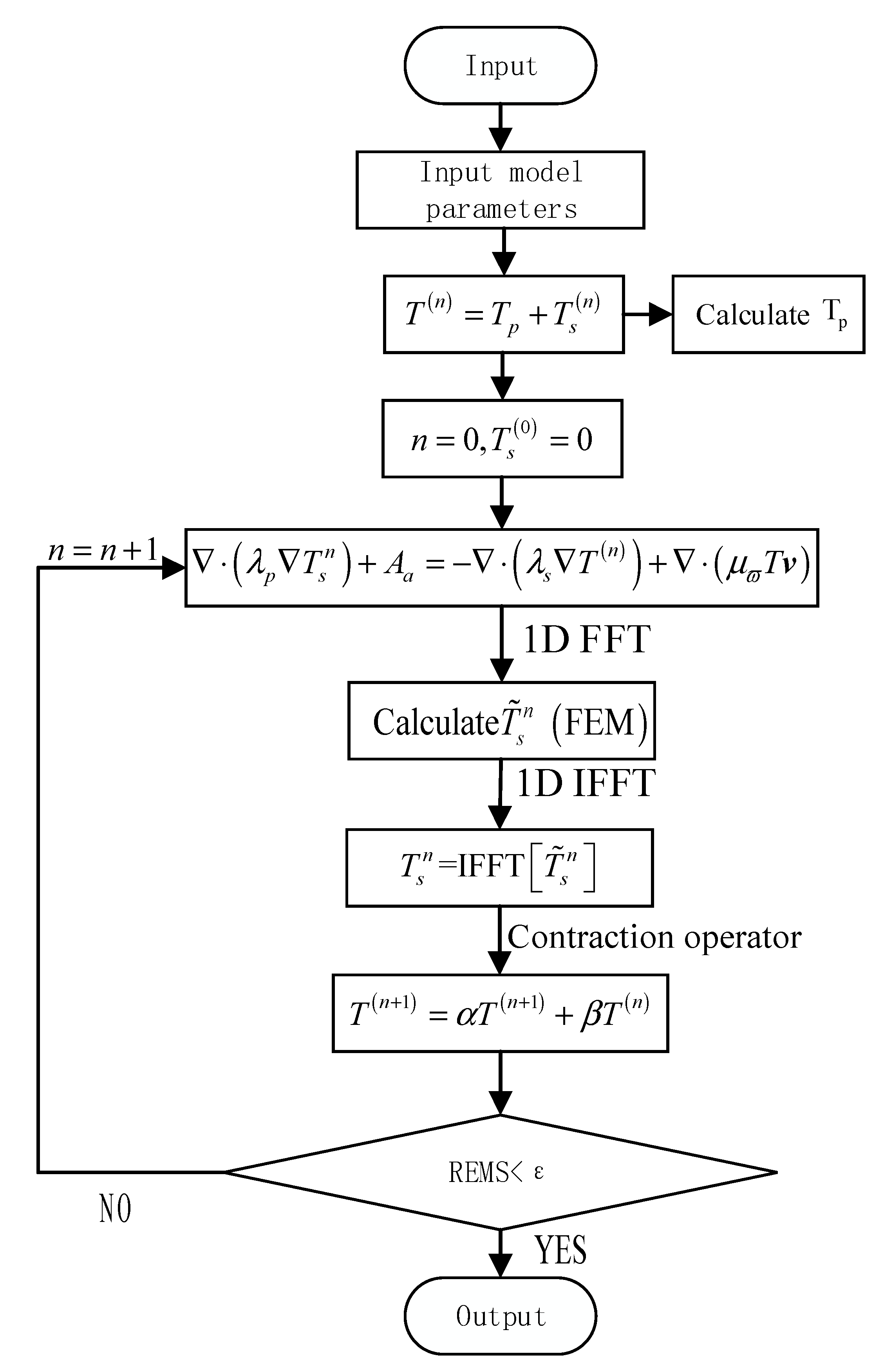
The specific steps of the proposed algorithm are described as follows:

Step 1: The model parameters are input, 2-D mesh generation is performed, sampling points in space domain $N_x,N_z$ are discretized, and sampling points in the wavenumber domain $k_x$ are obtained using the sampling theorem.

Step 2: Equation (2) is calculated using the finite element method, background temperature field $T_0$ is obtained, and $T_0$ is considered as the initial value of the total temperature field in the first iteration.

Step 3: Anomalous temperature field in the mixed space–wavenumber domain ${\tilde{T}}_s^n$ is calculated by solving Equation (3).

Step 4: Anomalous temperature field in the space domain $T_s^n$ is obtained using a 1-D inverse Fourier transform.

Step 5: A compact operator is applied, and total temperature field $T^{n+1}$ is updated.

Step 6: The relative root–mean–square error is determined. If $\mathit{RMSE}=\sqrt{{\displaystyle \frac{{\displaystyle \sum ^{N_{\mathrm{z}}}{\displaystyle \sum ^{N_{\mathrm{y}}}{\displaystyle \sum ^{N_{\mathrm{x}}}{\left(T^{\left(n+1\right)}{|}_{t=t_1}-T^{\left(n\right)}{|}_{t=t_1}\right)}^2}}}}{N_x{N}_y{N}_z}}}<\epsilon$, then the results are output. Otherwise, Step 3 is repeated until the accuracy requirement is satisfied. The error in this study is less than 0.1%.

The algorithm flowchart is shown in Figure 2.

5. Accuracy Validation

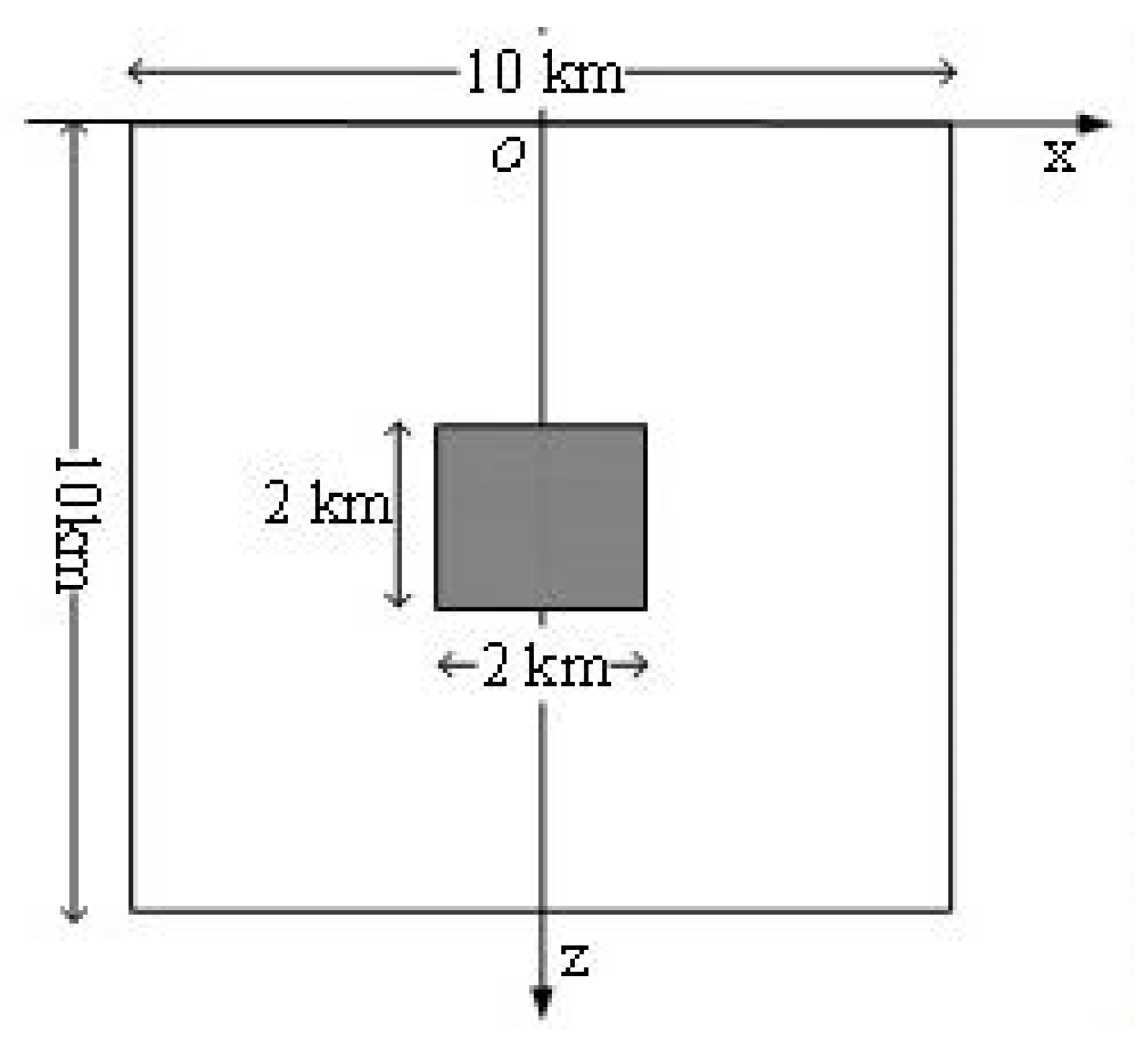
We designed a prism model with high thermal conductivity and compared the results of the algorithm in this paper with the calculation results of COMSOL Multiphysics finite element analysis software to verify the correctness of the algorithm.

The high thermal conductivity prismatic model is shown in Figure 3. The background thermal conductivity is $2 \mathrm{W}/\left(\mathrm{m}\cdot °\mathrm{C}\right)$, with no radiogenic heat production. There are prism anomalies with a side length of 2 km at the center of the calculated region, and the anomalous thermal conductivity is $6 \mathrm{W}/\left(\mathrm{m}\cdot °\mathrm{C}\right)$. The calculation region of the model is −5~5 km in the x direction and 0~10 km in the z direction. The first type of boundary condition is used for the upper boundary; the temperature is 10 °C. The lower boundary also adopts the first kind of boundary condition; the temperature is 164 °C. The grid nodes are 101 × 101. 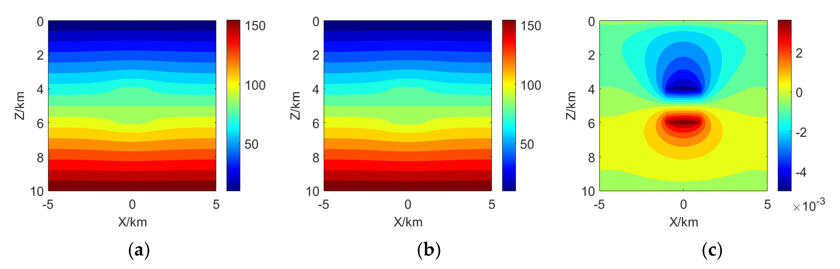Figure 4 presents the computational results of the proposed algorithm (a) and COMSOL Multiphysics (b) for the model shown in Figure 3, along with the relative error of the proposed algorithm’s results compared to those of COMSOL Multiphysics (c). From the relative error distribution map (Figure 4c), it can be observed that the maximum relative error between the computational results of the proposed algorithm and those of COMSOL Multiphysics for the model in Figure 3 does not exceed 0.5%, confirming the accuracy and correctness of the proposed algorithm.

6. Calculation Efficiency

Under the condition of consistent mesh size and model parameters, the computational time and memory usage of the proposed algorithm were compared with those of the finite element software COMSOL Multiphysics version 5.5 for different grid sizes.

The test platform is configured to consist of CPU-Intel(R) Core I5-9300h. The main frequency is 2.40 GHz, and the memory is 16 GB.

Table 1. Comparison of computational efficiency for different grid sizes.

Split Nodes	Total Nodes	Total Times (s)		Memory Occupied (GB)
		Algorithm of This Article	COMSOL Multiphysics	Algorithm of his Article	COMSOL Multiphysics
21 $\times$ 21	441	0.008	5	0.005	1.23
51 $\times$ 51	2601	0.04	6	0.015	1.33
101 $\times$ 101	10201	0.062	7	0.08	1.38
201 $\times$ 201	40401	1.18	9	0.18	1.78
401 $\times$ 401	160801	2.48	11	0.68	2.8

presents the computational time and memory usage of the proposed algorithm and the finite element software COMSOL Multiphysics for different grid sizes.

Figure 5 shows the line charts of the required time and memory usage (data sourced from Table 1). It can be observed that, under the same grid size, the proposed algorithm requires less computational time and memory usage compared to COMSOL Multiphysics. Moreover, the advantage of the proposed algorithm becomes more pronounced as the number of nodes increases.

7. Convergence Analysis

Using the same model configuration as that used in the accuracy validation, with the background thermal conductivity set to ${\lambda }_b$, this study investigates the influence of anomalous thermal conductivity on the convergence behavior of the iterative algorithm under varying numerical parameterizations. Specifically, high-conductivity anomalies $\left({\lambda }_s=5{\lambda }_b,10{\lambda }_b,50{\lambda }_b,100{\lambda }_b,500{\lambda }_b\right)$ and low-conductivity anomalies $\left({\lambda }_b=5{\lambda }_s,10{\lambda }_s,50{\lambda }_s,100{\lambda }_s,500{\lambda }_s\right)$ are defined to evaluate the iteration count required to achieve the preset computational tolerance $\left(\epsilon =0.005\right)$.

Analysis of the data in

Table 2. High thermal conductivity anomaly and iteration count.

Background-to-anomalous thermal conductivity ratio	1:5	1:10	1:50	1:100	1:500
Anomalous thermal conductivity $(\mathrm{W}/\left(\mathrm{m}\cdot °\mathrm{C}\right))$	10	20	100	200	1000
iteration count	3	5	17	32	167

and

Table 3. Low thermal conductivity anomaly and iteration count.

Background-to-anomalous thermal conductivity ratio	5:1	10:1	50:1	100:1	500:1
Anomalous thermal conductivity $(\mathrm{W}/\left(\mathrm{m}\cdot °\mathrm{C}\right))$	0.4	0.2	0.04	0.02	0.004
iteration count	2	3	7	13	43

indicates that the iteration count required to achieve the preset computational tolerance increases with the contrast between anomalous and background thermal conductivity, while stable convergence is consistently achieved. Furthermore, low-conductivity anomalies require fewer iterations and exhibit faster convergence compared to high-conductivity anomalies. The defined thermal conductivity contrasts cover the majority of scenarios encountered in practical geological settings, demonstrating the algorithm’s broad applicability in numerical simulations of geothermal fields.

8. Model Example

8.1. Cylinder Model

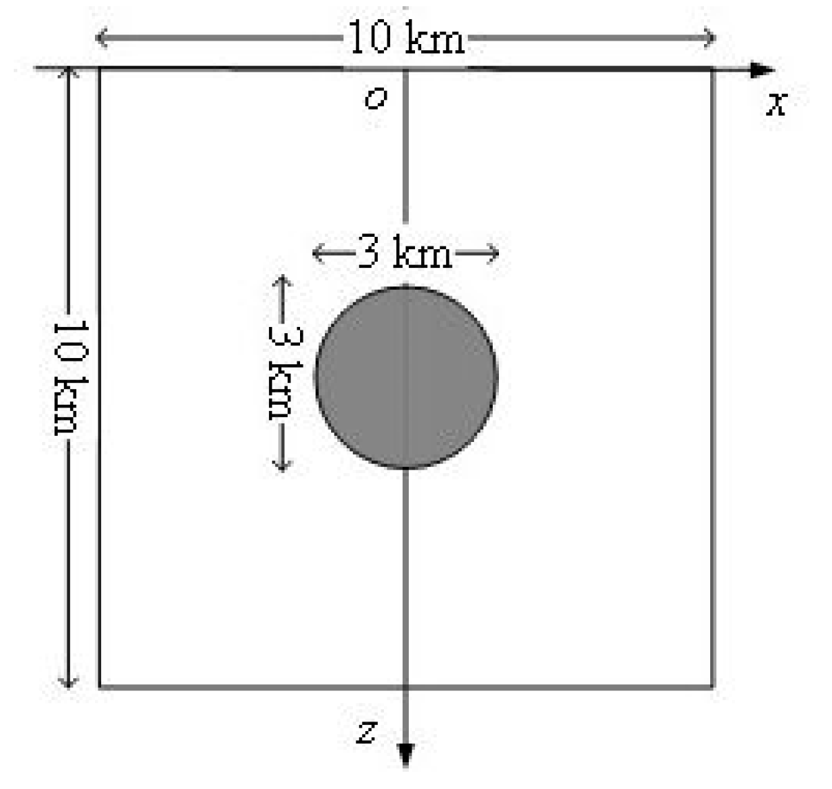
A cylindrical anomaly model with both high thermal conductivity and low thermal conductivity was designed to simulate the effects of thermal anomalies in a uniform background medium. The model geometry is illustrated in Figure 6.

The background of the model is a uniform half-space medium, the background thermal conductivity is $2 \mathrm{W}/\left(\mathrm{m}\cdot °\mathrm{C}\right)$, and there is no radiogenic heat production. There are spherical anomalies with a radius of 1.5 km at the center of the calculation area, and the distribution of the ground temperature field when the thermal conductivity of the anomalies body is $6 \mathrm{W}/\left(\mathrm{m}\cdot °\mathrm{C}\right)$ and $0.5 \mathrm{W}/\left(\mathrm{m}\cdot °\mathrm{C}\right)$ are calculated, respectively. The calculation area of the model is −5~5 km in the x direction and 0~10 km in the z direction. The first type of boundary condition is used for the upper boundary; the temperature is 10 °C. The second type of boundary condition is adopted for the lower boundary, and the heat flux value is $41.86 \mathrm{mW}/{\mathrm{m}}^2$. The grid nodes are 101 × 101.

The model calculation results are shown in Figure 7. The anomalous internal temperature isoline of a cylinder with low thermal conductivity is denser, and the heat flux and geothermal gradient are both larger than that of the background medium. The internal temperature isoline of a cylinder with high thermal conductivity is sparser, the heat flux and geothermal gradient are lower than that of the background medium, and the heat flux of the same magnitude exists at the same buried depth. The barrier effect of the anomalies body with low thermal conductivity on the heat flow is stronger than that of the cylinder with high thermal conductivity. The lower part near the heat flow is relatively higher, while the upper part away from the heat flow is lower.

8.2. Complex Model of High and Low Thermal Conductivity Combination

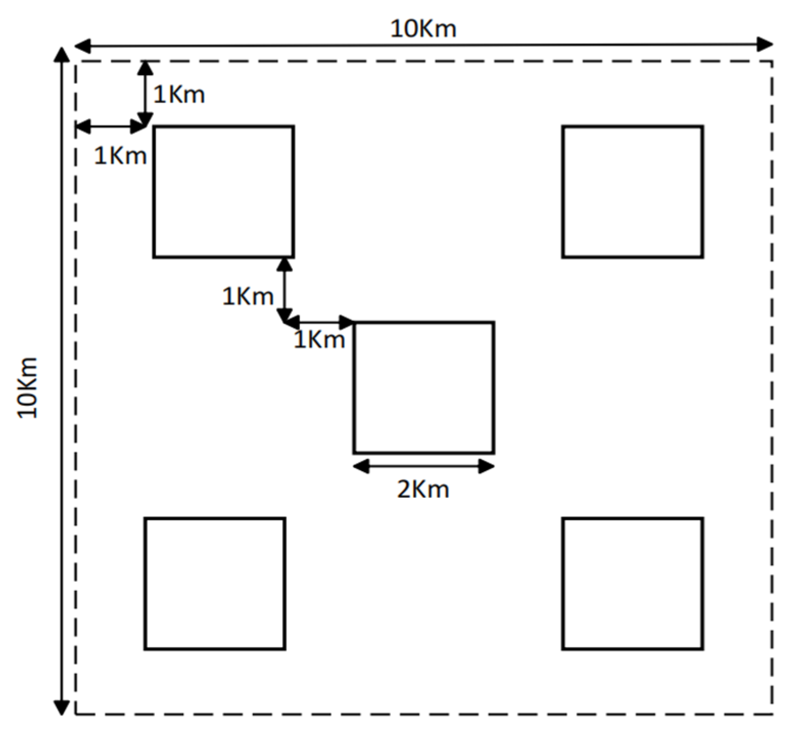
In order to verify that the algorithm can still accurately simulate the distribution of ground temperature field in the face of relatively complex underground media, a complex model with high and low thermal conductivity was set, as shown in Figure 8.

The background of the model is a uniform half-space medium, the background thermal conductivity is $2 \mathrm{W}/\left(\mathrm{m}\cdot °\mathrm{C}\right)$, and there is no radiogenic heat production. There are prismatic anomalies with a radius of $2 \mathrm{Km}$ in the center of the space and in all surrounding positions. The distance between the peripheral anomalies and the adjacent boundaries is $1 \mathrm{Km}$, and the horizontal and vertical distance between the central prism and the peripheral anomalies is $1 \mathrm{Km}$. The central anomalies body is the anomalous body with high thermal conductivity and thermal conductivity is $6 \mathrm{W}/\left(\mathrm{m}\cdot °\mathrm{C}\right)$, and the surrounding anomalies body with low thermal conductivity is $0.5 \mathrm{W}/\left(\mathrm{m}\cdot °\mathrm{C}\right)$. The calculation area of the model is −5~5 km in the x direction and 0~10 km in the z direction. The first type of boundary condition is used for the upper boundary, the temperature is 10 °C; The second type of boundary condition is adopted for the lower boundary, and the heat flux value is $41.86{ \mathrm{mW}/\mathrm{m}}^2$. The grid nodes are 101 × 101.

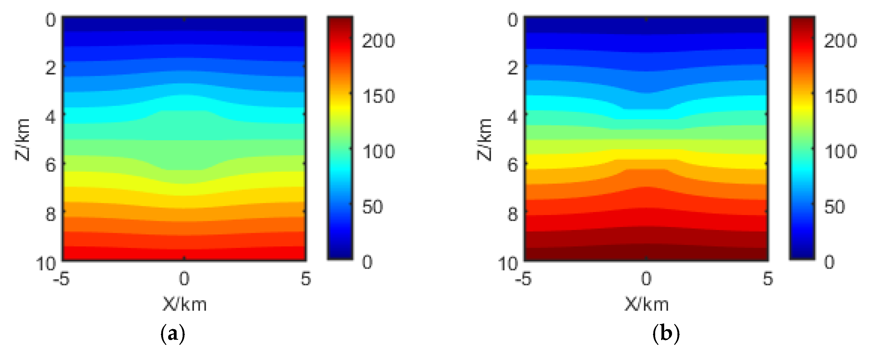
The calculated results of the model are shown in Figure 9. It can be seen that the isolines inside the central prism with high thermal conductivity are more sparse, and the isolines inside the anomalies body with low thermal conductivity around it are more dense. Moreover, the proposed algorithm can still reflect the location of the anomalies body through isoline distribution in the face of the complex distribution of underground media, and effectively and accurately simulate the distribution of temperature field in space.

8.3. Rolling Terrain Model

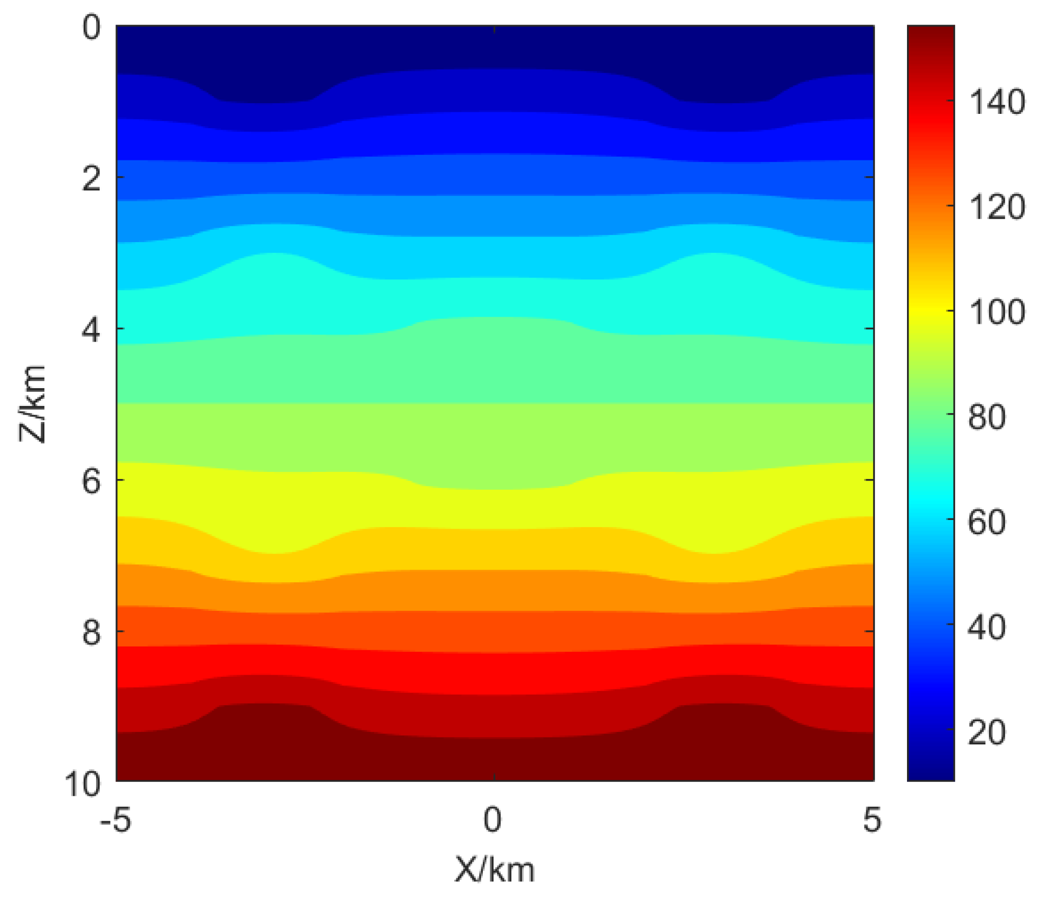
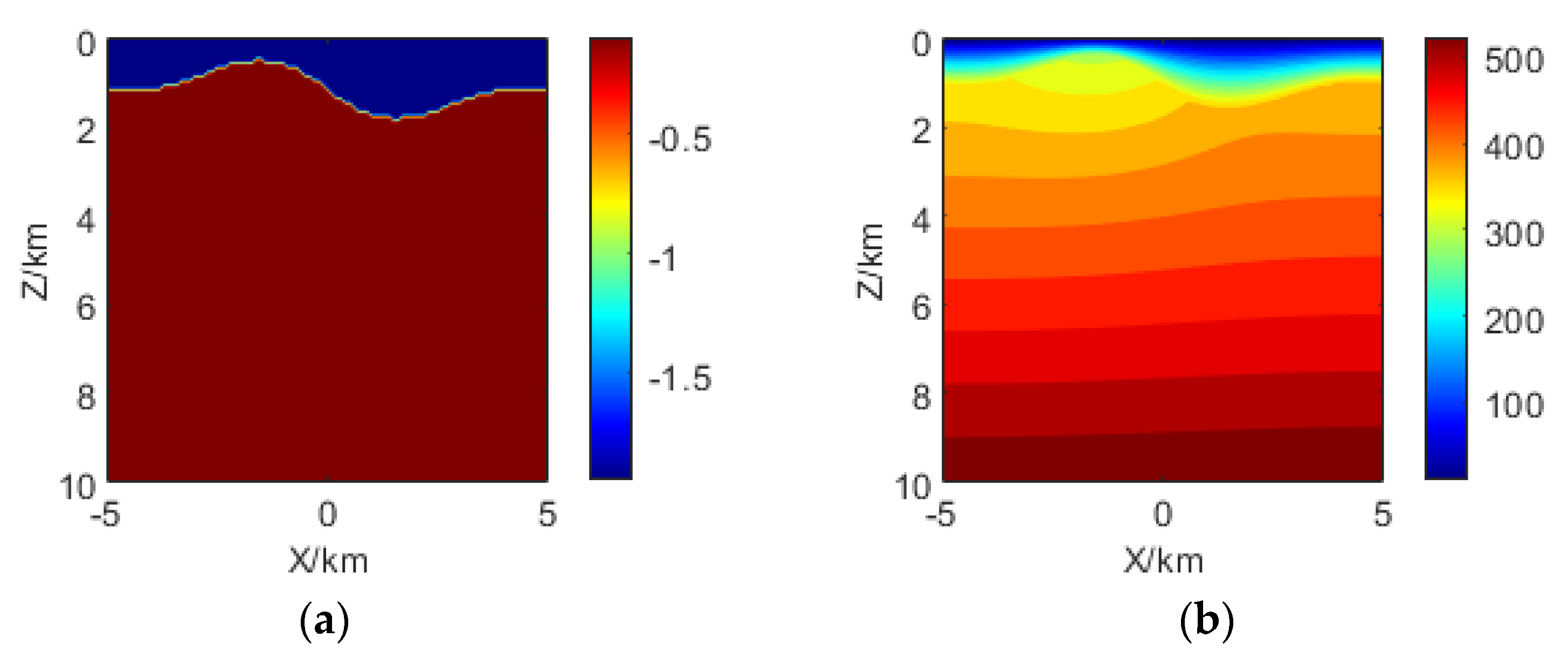
We set the undulating terrain model. The undulating terrain is shown in Figure 10. The function expression satisfied by the terrain is $z={\displaystyle \frac{1}{2}}\left(5000-\left|x\right|\right)\sin \left({\displaystyle \frac{x}{400\pi }}\right)$. The background of the model is a uniform half-space medium with a background thermal conductivity of $2 \mathrm{W}/\left(\mathrm{m}\cdot °\mathrm{C}\right)$ and no radiogenic heat production. The anomalies body is air with a thermal conductivity of $0.05 \mathrm{W}/\left(\mathrm{m}\cdot °\mathrm{C}\right)$. The calculation area of the model is −5~5 km in the x direction and 0~10 km in the z direction. The first type of boundary condition is used for the upper boundary; the temperature is 10 °C. The second type of boundary condition is adopted for the lower boundary, and the heat flux value is $41.86{ \mathrm{mW}/\mathrm{m}}^2$. The grid nodes are 101 × 101.

It can be seen from the simulation results that, compared with the low-lying region, the temperature in the high-lying region is more affected by terrain and thus the temperature is lower. Moreover, the influence of terrain on temperature field gradually decreases with the increase in depth.

9. Conclusions

For the present numerical simulation methods of ground temperature field, in order to achieve high precision in the face of a large medium scale, it is often necessary to carry out fine subdivision of the model, which has a large number of subdivision units, and has problems such as large memory consumption and long calculation times. In this paper, a method is proposed using a spatial and wavenumber mixed domain numerical simulation method of ground temperature field. This method will meet the two-dimensional differential equation along the horizontal direction of one-dimensional Fourier transform into different wavenumbers of independent one-dimensional ordinary differential equation, and decompose a large-scale two-dimensional numerical simulation problem into multiple one-dimensional numerical simulation problems, greatly reducing the amount of calculation and storage needed. The high efficiency and high precision numerical simulation of 2D geothermal field is realized. In this paper, several models are designed to verify the correctness and effectiveness of the algorithm and its adaptability to complex geological models (complex structure, undulating terrain, etc.). Comparing the computational efficiency with the finite element software COMSOL Multiphysics, the results show that the time and memory requirements of the spatial wavenumber domain algorithm under the same mesh generation conditions are reduced by 1 to 2 orders of magnitude, and the numerical simulation of more sophisticated and complex models has more obvious advantages. The results of this study can provide important numerical research tools for evaluating geothermal resources, exploitation and utilization of geothermal energy, and inversion interpretation. However, since the algorithm computes steady-state geothermal fields, it lacks the capability to analyze dynamic variations in geothermal temperature distributions. Additionally, although complex geological models and undulating terrain models were designed to validate the algorithm’s applicability to complex geological conditions and its potential for practical applications, further validation using real-world geological data is still required to assess its robustness in addressing real geological challenges.