Variation in Electron Radiation Properties Under the Action of Chirped Pulses in Nonlinear Thomson Scattering

Abstract

This paper primarily focuses on the changes in electron motion trajectories, radiation spatial distribution, radiation spectra, and time spectra under the combined influence of pulse width and chirp parameters. It discusses the motion characteristics of electrons in Gaussian circularly polarized laser-chirped pulses with different chirp parameters and pulse widths. This study examines the asymmetry in radiation distribution, the increase in peak power, the time adjustment in main peak generation, and the coupling effects of spatial distribution under the combined action of pulse width and chirp parameters. It also explores the similarity between chirp effects and pulse broadening. Overall, this paper provides an important reference for further understanding and applying chirped pulses in optics and physics by deeply studying the characteristics of electrons under varying conditions of chirp parameters and pulse widths.

1. Introduction

Chirped pulse is a special form of laser pulse whose frequency varies with time. Chirped pulses usually are characterized by linear frequency modulation, that is, the frequency at which the pulse begins is different from the frequency at which it ends, resulting in a broadband spectrum. One of the characteristics of a chirped pulse is that its phase changes linearly with time, and this change results in a change in frequency. Chirped pulse has a characteristic of large bandwidth and short duration in spectrum, which makes it widely used in ultrafast spectroscopy and laser spectroscopy. In a chirped pulse, the rate of frequency change is called the Chirp Rate parameter and is usually expressed as the absolute value of the rate of frequency change. The chirp rate of a chirped pulse can be positive (gradually increasing in frequency) or negative (gradually decreasing in frequency), depending on how the pulse is modulated [1,2,3,4,5].

First proposed in the 1990s, chirped pulses have significant application potential in ultrafast laser spectroscopy, optical coherence tomography (OCT) [6], fiber optic communication [7,8] and other fields. Since 1992, when optical parametric amplification proved the principle of effectively amplifying chirped laser pulses, optical parameter chirped pulse amplification (OPCPA) has become the most promising method for broadband optical pulse amplification. At the same time, we are witnessing exciting progress in the development of powerful ultrashort-pulse laser systems with chirped-pulse parametric amplifiers. The output power and pulse duration of these systems range from a few gigawatts to hundreds of terawatts, with potential power levels reaching tens of petawatts [9]. They are capable of providing broader spectrum coverage than conventional pulses, thus performing exceptionally well in applications requiring high resolution and sensitivity. For example, Hu et al. [10] proved that the bandwidth and duration of the incident pulsed beam play an important role in the correction of nonlinear images of amplitude-type scatterers. At the same time, chirped pulses also have a significant demand for high-power, high-intensity laser pulses in areas such as particle laser acceleration. Maher, Singh [11,12,13,14,15] et al. pointed out that high-intensity pulses play an important role in electronic trajectory control and state change. The chirped-pulse amplification technology also has great advantages in the generation of high-power and high-intensity pulses and electronic control at the nanoscale, and the effect is better than that of traditional large instruments [16,17,18].

The spatial radiation characteristics of pulses can be divided into linear polarization, circular polarization, and elliptic polarization based on the state of space radiation. Due to the complexity of chirped laser pulse analysis, most studies are conducted under the condition of online polarization or the chirped amplification effect using different crystal materials. For example, Gupta et al. [1,19] qualitatively analyzed the influence of linear polarization on chirped-laser-pulse single-electron acceleration and its related effects on electron dynamics. Hu et al. [20] studied the dynamics of single electrons directly accelerated by linearly polarized chirped laser pulses in an inhomogeneous cylindrical plasma channel. Tan et al. [21] studied the ionization dynamics of atoms with chirped-attosecond pulses. Wu et al. [22] studied the high-order harmonic generation cutoff extension of strongly few-cycle linearly chirped laser pulses. Wang et al. [23] mainly studied optical parametric chirped-pulse amplification based on photonic crystal fiber. Due to the axisymmetric nature of the circularly polarized laser field, it provides a better acceleration effect. Additionally, circularly polarized laser pulses can drive electrons to move in three-dimensional space, allowing for more detailed data and parameters on the radiation spatial distribution and motion trajectories of the electrons. This provides a better data reference for controlling electron motion with high-energy laser pulses. Therefore, this paper presents numerical simulations and result analyses of the radiation spatial distribution and motion trajectories of stationary electrons driven by circularly polarized chirped pulses.

Jisrawi et al. [24,25] analyzed the fluctuation effect of energy gain as a result of changing the chirped parameter. However, the cross-effects of chirped parameters and other pulse-related parameters, such as pulse width, have not been studied too much. This paper builds upon the findings of Kumar et al. and investigates the combined effect of the chirp parameter and pulse width. [26] Considering the high costs associated with the instruments, manpower, and material preparation required for conducting nonlinear Thomson scattering experiments, as well as the difficulty in performing large-scale experiments on individual electrons, simulations through computational experiments offer a more efficient approach. Such simulations allow for large-scale data acquisition and analysis in a relatively shorter time and at a lower cost. Therefore, the simulation of nonlinear Thomson scattering and the subsequent data analysis through simulations hold significant research value. Moreover, many scholars have also studied nonlinear Thomson scattering under different conditions. [27,28,29] For the first time, this paper conducts a systematic analysis of the interaction between laser pulses and electrons under different chirp parameters and pulse width conditions. It details the electron motion trajectories in multiple states, providing theoretical guidance for the experimental design and phenomenon analysis of laser pulse and free electron interactions. The relative changes in electron dynamic characteristics under different combination conditions of pulse width and chirp parameters are studied.

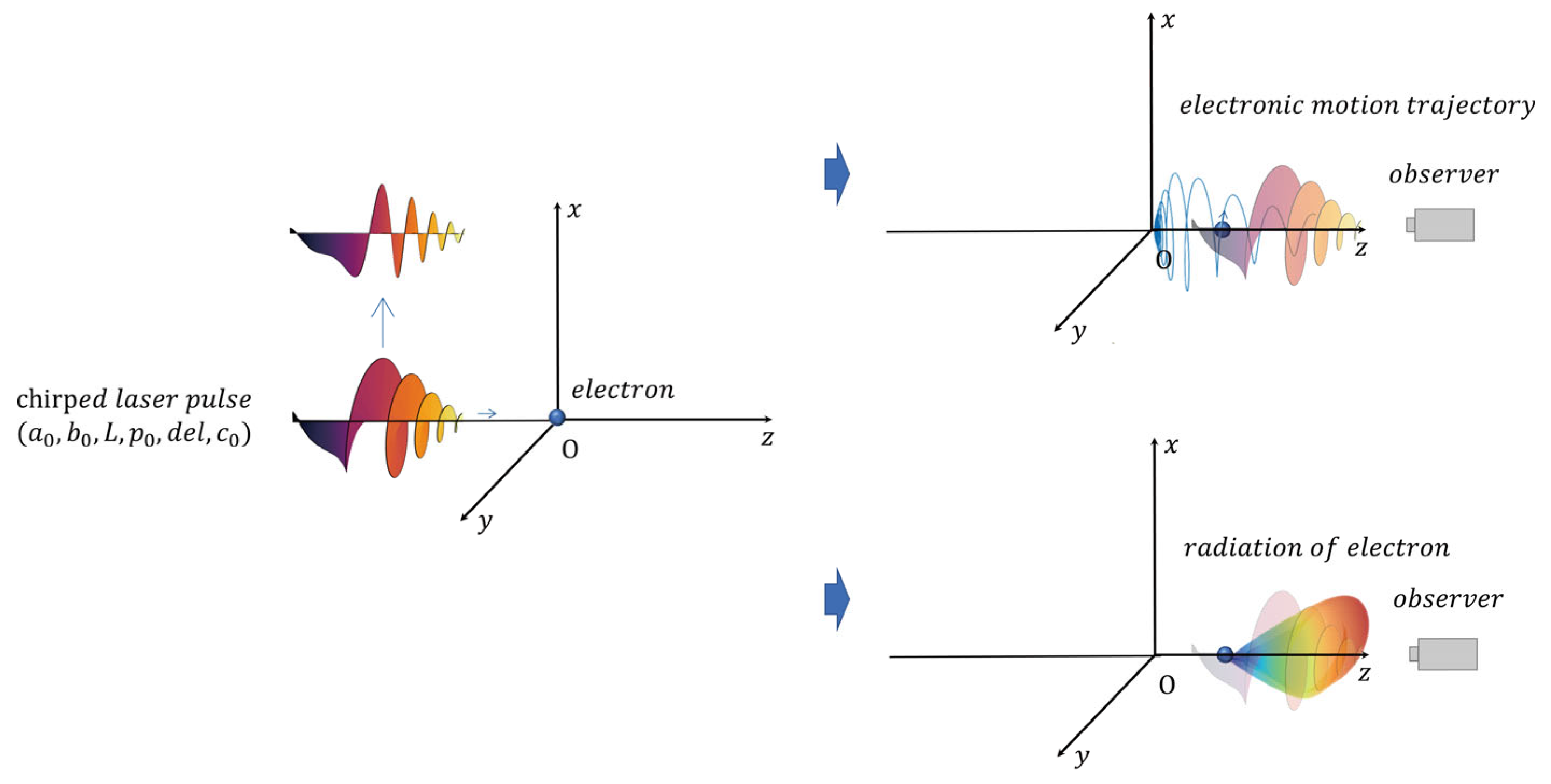
2. Materials and Methods

In terms of data processing, all physical variables were normalized by $k_0^{-1}={\lambda }_0/2\pi$ and ${\omega }_0^{-1}={\lambda }_0/2\pi c$, where ${\lambda }_0=1 \mathsf{\mu }\mathrm{m}$ is the wavelength of the laser and $c=2.998\times {10}^8 \mathrm{m}/\mathrm{s}$ is the speed of light. This paper not only uses the observer as a reference, defining $t$ as the time on the observer system, but also introduces the electronic reference frame, defining the time as $t_e=t-R^{\prime }+\mathit{n}·\mathit{j}$ with the electron as the reference frame, where $R^{\prime }$ is the distance between the observer and the interaction center, and $\mathit{j}=(x_{t_e},y_{t_e},z_{t_e})$ is the electron displacement at $t_e$ time. Radiation direction $\mathit{n}=(\sin \theta \cos \varphi ,\sin \theta \sin \varphi ,\cos \theta )$, where $\theta$ is the polar angle, and $\varphi$ is the azimuth angle. The initial electron position $(x_0,y_0,z_0)$ is set to $(0,0,0)$ to ensure that the pulse and electron begin to interact at the origin [30].

The chirped pulse and electron action process are shown in Figure 1. The initial position of the laser is on the negative half of the z-axis, propagating along the positive z-axis at the speed of light $c$, interacting with the stationary electron at the origin and driving the electron’s motion. In a tightly focused Gaussian laser field, the electric field $\mathit{E}$ and magnetic field $\mathit{B}$ satisfying Maxwell’s equations can be expressed as follows [31]:

$$\mathit{E}=\nabla \times \mathit{A}$$

(1)

$$\mathit{B}=\sqrt{ϵ}[(i/k)\nabla (\nabla ·\mathit{A})+ik\mathit{A}]$$

(2)

where $ϵ$ is the dielectric constant, we can use Helmholtz’s equation to obtain the solution for $\mathit{A}$:

$${\nabla }^2\mathit{A}+k_0^2\mathit{A}=0$$

(3)

In Cartesian coordinates, a circularly polarized laser can be decomposed into a pair of linearly polarized lasers with phase difference $\pi /2$, whose polarization planes are parallel to $x$ and $y$, respectively. Therefore, the electromagnetic field circularly polarized laser can be decomposed into $\mathit{E}={\mathit{E}}_{\mathit{x}\mathit{p}}+{\mathit{E}}_{\mathit{y}\mathit{p}}$ and $\mathit{B}={\mathit{B}}_{\mathit{x}\mathit{p}}+{\mathit{B}}_{\mathit{y}\mathit{p}}$. The spot size of the Gaussian laser field in this model is $2w_0$, the pulse width $L$ and the intensity $I$, so we can define

$$E_0=a_0{\displaystyle \frac{w_0}{w}}\exp \left(-{\displaystyle \frac{{\eta }^2}{L^2}}\right)\exp \left(-{\displaystyle \frac{{\rho }^2}{w^2}}\right)$$

(4)

where $a_0=\sqrt{(I{\lambda }_0^2/1.384)}\times {10}^{-9}$ is the peak amplitude, $w=w_0 \sqrt{(1+z^2/z_0^2)}$ is the waist radius, and where Rayleigh’s distance $z_0=k_0{w}_0^2/2$. The perpendicular distance $\eta =z-ct$, the parallel distance $\rho =\sqrt{(x^2+y^2)}$, and the speed of light is $c$. In the case of tight laser focus, the expression of the electromagnetic field must be expanded to a higher order, accurate to the diffraction angle $\epsilon =w_0/z_0$. Yousef et al. [32] derived $\mathit{A}$, $\mathit{B},$ and $\mathit{E}$ in the X-axis polarization laser field from Equation (1) to Equation (3). Zhang [33] and Barton [31] proposed an electromagnetic field expression for a Y-axis polarized laser field by using a symmetric expression. In summary, the fifth-order expansion of the electric field component $\mathit{E}=\{E_x,E_y,E_z\}$ can be obtained:

$$\begin{array}{c}{E}_x=E_0\{S_0+{\epsilon }^2[{\alpha }^2{S}_2-{\displaystyle \frac{r^4{S}_3}{4}}] \\ +{\epsilon }^4\left[{\displaystyle \frac{S_2}{8}}-{\displaystyle \frac{r^2{S}_3}{4}}-{\displaystyle \frac{r^2\left(r^2-16{\alpha }^2\right)S_4}{16}}-{\displaystyle \frac{r^4\left(r^2+2{\alpha }^2\right)S_5}{8}}+{\displaystyle \frac{r^8{S}_6}{32}}\right]\\ +{\epsilon }^2{C}_2+{\epsilon }^4[r^2{C}_4-{\displaystyle \frac{r^4{C}_5}{4}}]\}\end{array}$$

(5)

$$\begin{array}{c}{E}_y=E_0\{C_0+{\epsilon }^2[{\beta }^2{C}_2-{\displaystyle \frac{r^4{C}_3}{4}}]\\ +{\epsilon }^4\left[{\displaystyle \frac{C_2}{8}}-{\displaystyle \frac{r^2{C}_3}{4}}-{\displaystyle \frac{r^2\left(r^2-16{\beta }^2\right)C_4}{16}}-{\displaystyle \frac{r^4\left(r^2+2{\beta }^2\right)C_5}{8}}+{\displaystyle \frac{r^8{C}_6}{32}}\right]\\ +{\epsilon }^2{S}_2+{\epsilon }^4[r^2{S}_4-{\displaystyle \frac{r^4{S}_5}{4}}]\}\end{array}$$

(6)

$$\begin{array}{c}\begin{array}{c}\begin{array}{c}\begin{array}{c}{E}_z=E_0\alpha \{\epsilon C_1+{\epsilon }^3[-{\displaystyle \frac{C_2}{2}}+r^2{C}_3-{\displaystyle \frac{r^4{C}_4}{4}}]\\ +{\epsilon }^5[-{\displaystyle \frac{3C_3}{8}}-{\displaystyle \frac{3r^2{C}_4}{8}}+{\displaystyle \frac{17r^4{C}_5}{16}}-{\displaystyle \frac{3r^6{C}_5}{16}}-{\displaystyle \frac{3r^6{C}_6}{8}}+{\displaystyle \frac{r^8{C}_7}{32}}]\}\end{array}\\ -E_0\beta \{\epsilon S_1+{\epsilon }^3[-{\displaystyle \frac{S_2}{2}}+r^2{S}_3-{\displaystyle \frac{r^4{S}_4}{4}}]\end{array}\\ +{\epsilon }^5[-{\displaystyle \frac{3S_3}{8}}-{\displaystyle \frac{3r^2{S}_4}{8}}+{\displaystyle \frac{17r^4{S}_5}{16}}-{\displaystyle \frac{3r^6{S}_5}{16}}-{\displaystyle \frac{3r^6{S}_6}{8}}+{\displaystyle \frac{r^8{S}_7}{32}}]\}\end{array}\end{array}$$

(7)

The components of a magnetic field are described as follows:

$$B_x=E_0\{C_0+{\epsilon }^2[{\displaystyle \frac{r^2{C}_2}{2}}-{\displaystyle \frac{r^4{C}_3}{4}}]+{\epsilon }^4[-{\displaystyle \frac{C_2}{8}}+{\displaystyle \frac{r^2{C}_3}{4}}+{\displaystyle \frac{5r^4{C}_4}{16}}-{\displaystyle \frac{r^6{C}_5}{4}}+{\displaystyle \frac{r^8{C}_6}{32}}]\}$$

(8)

$$B_y=E_0\{S_0+{\epsilon }^2[{\displaystyle \frac{r^2{S}_2}{2}}-{\displaystyle \frac{r^4{S}_3}{4}}]+{\epsilon }^4[-{\displaystyle \frac{S_2}{8}}+{\displaystyle \frac{r^2{S}_3}{4}}+{\displaystyle \frac{5r^4{S}_4}{16}}-{\displaystyle \frac{r^6{S}_5}{4}}+{\displaystyle \frac{r^8{S}_6}{32}}]\}$$

(9)

$$\begin{array}{c}{B}_z=E_0\beta \left\{\epsilon C_1+{\epsilon }^3[{\displaystyle \frac{C_2}{2}}+{\displaystyle \frac{r_2{C}_3}{2}}-{\displaystyle \frac{r_4{C}_4}{4}}]+{\epsilon }_5[{\displaystyle \frac{3C_3}{8}}+{\displaystyle \frac{3r^2{C}_4}{8}}+{\displaystyle \frac{3r^4{C}_5}{16}}-{\displaystyle \frac{r^6{C}_6}{4}}+{\displaystyle \frac{r^8{C}_7}{32}}]\right\}\\ -E_0\alpha \left\{\epsilon S_1+{\epsilon }^3[{\displaystyle \frac{S_2}{2}}+{\displaystyle \frac{r_2{S}_3}{2}}-{\displaystyle \frac{r_4{S}_4}{4}}]+{\epsilon }_5[{\displaystyle \frac{3S_3}{8}}+{\displaystyle \frac{3r^2{S}_4}{8}}+{\displaystyle \frac{3r^4{S}_5}{16}}-{\displaystyle \frac{r^6{S}_6}{4}}+{\displaystyle \frac{r^8{S}_7}{32}}]\right\}\end{array}$$

(10)

where $\alpha =x/w_0$, $\beta =y/w_0$, $r=\rho /w_0$. $S_m$ and $C_m$ are shown below:

$$S_m={\left({\displaystyle \frac{w_0}{w}}\right)}^m\sin \left(\psi +m{\psi }_G\right)$$

(11)

$$C_m={\left({\displaystyle \frac{w_0}{w}}\right)}^m\cos \left(\psi +m{\psi }_G\right)$$

(12)

$$m=\mathrm{0,1},2,\dots$$

It is worth noting that in the formula, the x and y components of E and B are expanded one order less than the z-component. This is because, in actual electromagnetic fields, the longitudinal components are an order of magnitude smaller than the transverse components.

The phase is as follows: $\psi ={\psi }_0+\eta -{\psi }_R+{\psi }_G+c_0{\eta }^2$, where $c_0{\eta }^2$ is the phase shift caused by the chirp, and the initial phase ${\psi }_0$ is the plane wave phase. ${\psi }_R={\rho }^2/2R\left(z\right)$ is the phase related to the curvature of the wavefront, and $R\left(z\right)=z+z_0^2/z$ represents the z coordinate of the radius of curvature where the wavefront intersects the beam axis. ${\psi }_G=ta{n}^{-1}(z/z_0)$ is an additional phase transition that a Gaussian beam undergoes, meaning that the Gaussian beam will undergo a total phase transition when changing from $-\infty$ to $+\mathrm{\infty }$.

Considering the rest mass of a single electron $m_e=9.1096\times {10}^{-31} \mathrm{k}\mathrm{g}$, charge $-e=-1.6022\times {10}^{-19}\mathrm{C}$, we use the following Lorentz equation and energy equation to determine and describe the motion state of the electron in the intense laser pulse

$${\displaystyle \frac{d\mathit{p}}{d{t}_e}}=-e\left(\mathit{E}+\mathit{u}\times \mathit{B}\right)$$

(13)

$${\displaystyle \frac{d\Gamma }{d{t}_e}}=-e\left(\mathit{v}·\mathit{E}\right)$$

(14)

where $\Gamma ={\gamma }_0{m}_e{c}^2$ represents the electron energy, defined by the formula ${\gamma }_0^{-1}=\sqrt{1-{\mathit{u}}^2}$, where ${\gamma }_0$ is the Lorentz factor and represents the normalized initial energy of the electron. Momentum of the electron $\mathit{p}=\Gamma \mathit{v}/c^2$, where $\mathit{v}$ is the electron velocity and $\mathit{u}=\mathit{v}/c$.

The time-varying electromagnetic field generated by moving charged particles can be derived from the Lenard–Wiechert potential [34], so the radiated power per unit solid angle can be calculated as:

$${\displaystyle \frac{dP\left(t_e\right)}{d\Omega }}={\left[{\displaystyle \frac{{|\mathit{n}\times [\left(\mathit{n}-\mathit{u}\right)\times d_t\mathit{u}]|}^2}{(1-\mathit{n}·\mathit{u}{)}^6}}\right]}_t$$

(15)

where the power of the radiation pulse $dP\left(t_e\right)/d\Omega$ is normalized to $e^2{\omega }_0^2/4\pi c$. The different time subscripts in Equation (15) indicate that the pulses received by the observer at time t are actually emitted by electrons at time $t_e$.

The Runge–Kutta–Fehlberg method (RKF45) is a numerical method used to solve ordinary differential equations. The RKF45 method automatically adjusts the computational accuracy through adaptive step sizes. It combines the fourth-order and fifth-order Runge–Kutta methods, allowing it to estimate errors during the computation and adaptively adjust the step size to meet the specified accuracy requirements [35,36]. We used the 4–5 Runge–Kutta–Fehlberg method (RKF45) to solve the ordinary differential Equations (13) and (14), and large-scale GPU parallel solutions were carried out on MATLAB R2023a to record the numerical solutions of electron positions, velocities, and accelerations at each step. The radiation of different space–time states could be obtained from Equation (15).

3. Results

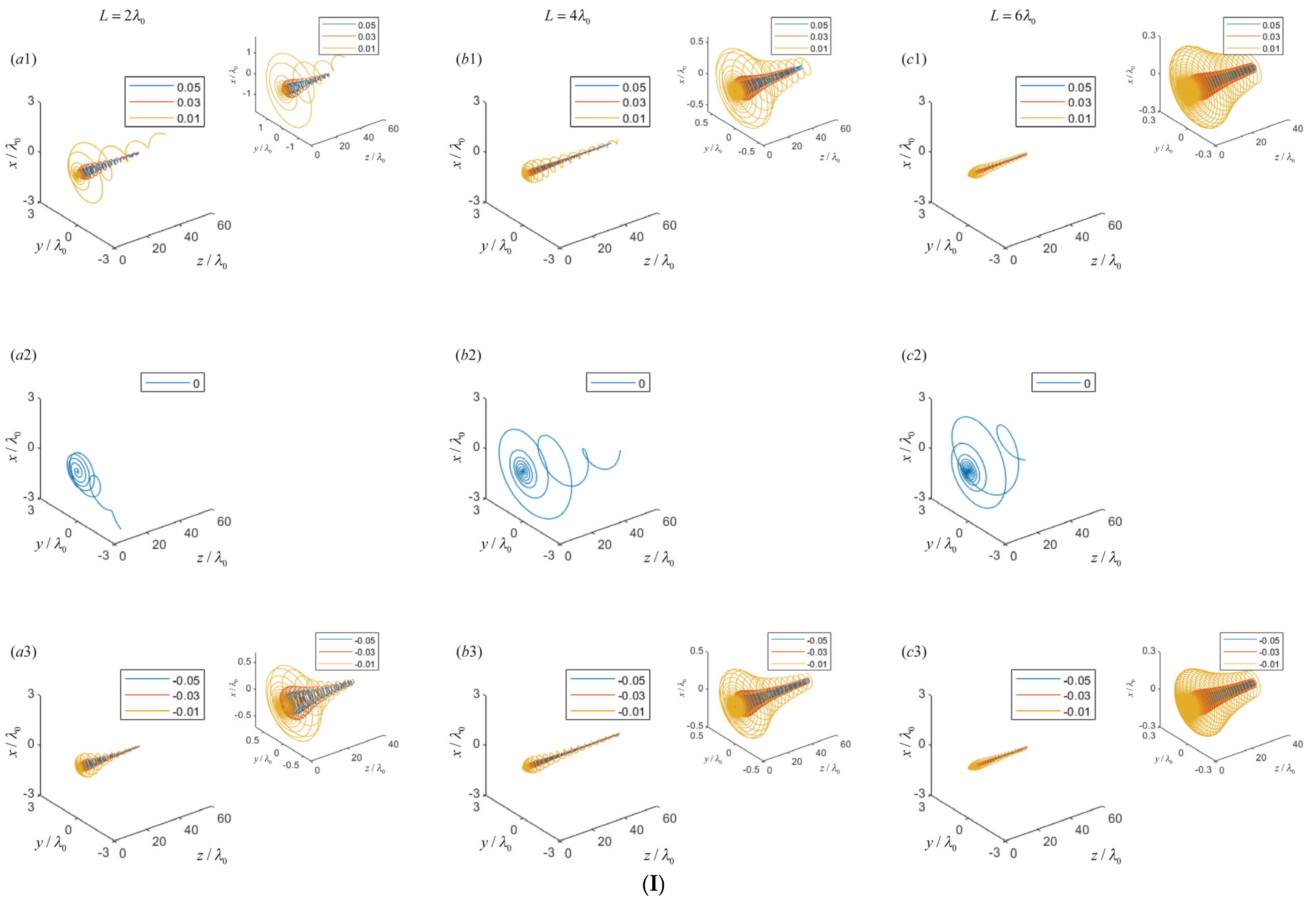
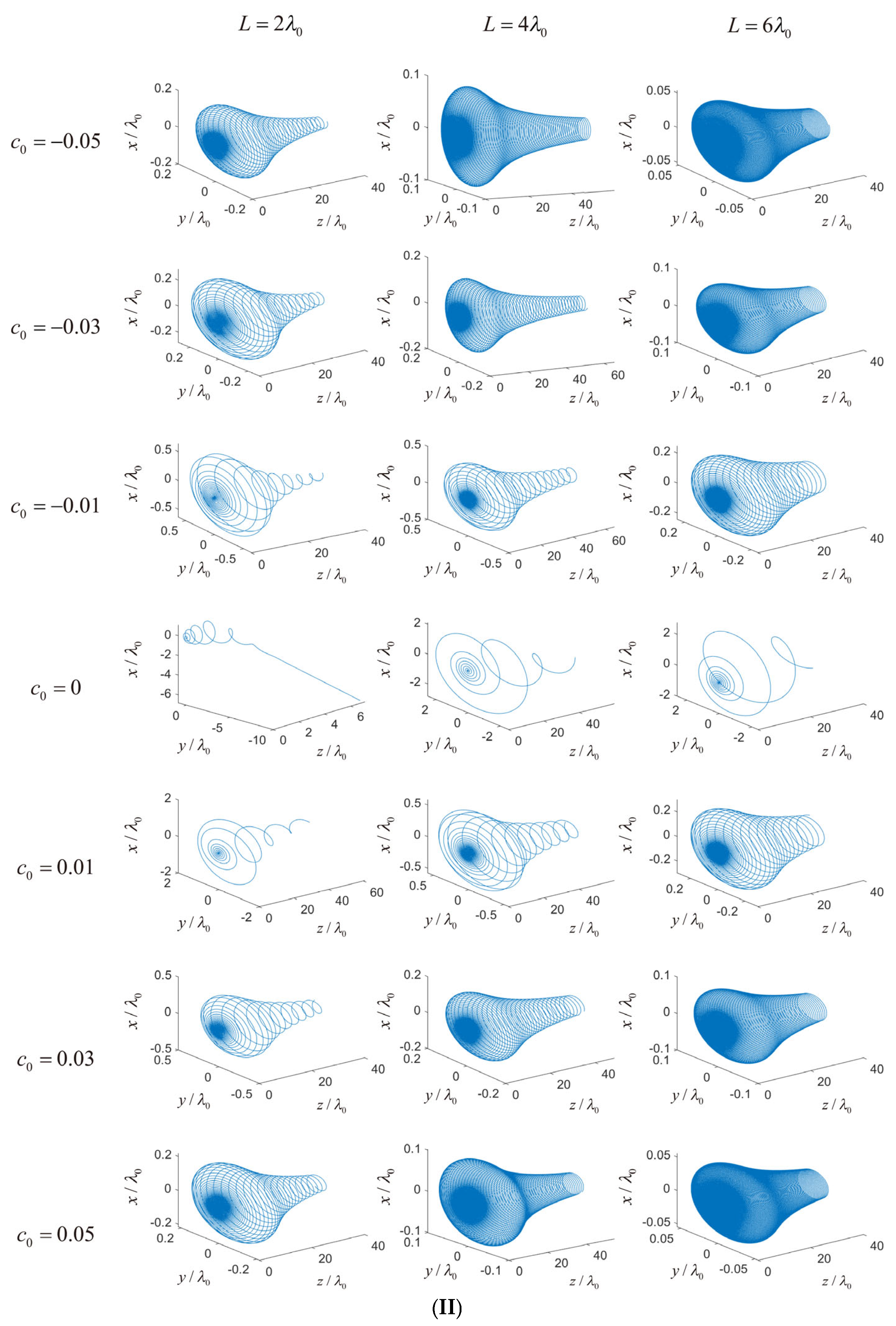
3.1. Motion Trajectory Analysis

An electron is fixed to the origin of the coordinate. The incident circularly polarized laser-chirped pulse is an electromagnetic wave whose transverse electric field and irradiance distribution approximately meet the Gaussian envelope, propagating along the +z-axis. Its wavelength is ${\lambda }_0=1 \mathsf{\mu }\mathrm{m}$ and its optical intensity parameter is $a_0=5 (the laser pulse intensity I=3.45\times {10}^{19} \mathrm{W}/\mathrm{c}{\mathrm{m}}^2)$, and the chirped pulse width $L$ is taken as three sets of values, which are $2{\lambda }_0,4{\lambda }_0, \mathrm{a}\mathrm{n}\mathrm{d} 6{\lambda }_0$, respectively. The corresponding pulse durations are $6.7 fs,13.3 fs, \mathrm{a}\mathrm{n}\mathrm{d} 20 fs$, and the waist radius $w_0$ is determined as $4 \mathsf{\mu }\mathrm{m}$. The chirped parameter $c_0$ changes from $-0.05$ to $+0.05$, and the electron motion, full-angle, and spectral characteristics of the electron radiation during the transition from compact-focused laser to non-compact-focused laser and even to the plane wave are studied. The environmental parameters are kept constant without being described otherwise and will not be described below.

Based on classical electrodynamics, we employed the fourth-order Runge–Kutta algorithm to solve the corresponding partial differential equations, obtaining the electron trajectory as shown in the figure. It can be seen from Figure 2 that the static electron, driven by the Gaussian circularly polarized laser-chirped pulse, first carries out a spiral motion similar to the isogonal spiral, and the change process of its pitch is basically consistent with the change process of the Gaussian function. According to the change, we can see that when the electron lags behind the end of the pulse-falling edge, the electron begins to perform a uniform linear motion.

We found that after the chirp parameter was added, the range of electron motion trajectory changed to a large extent. In order to visually display the change in motion trajectory and facilitate a comparison, we placed the axis of motion trajectory under the same axis in the comparison chart. Due to the effect of the chirp parameter, the electron motion trajectory contracted too much. In Figure 2I(a1–c1,a3–c3), a clearer motion trajectory is attached to the upper right corner of the six pictures, which is convenient when showing the change in motion trajectory of the chirped pulse under the same pulse width.

It can be seen from the motion trajectory in Figure 2I that the radial motion radius of the electron without chirp influence is larger than that of the trajectory with chirp influence. The radial trajectory envelope of electron motion is very similar to that of the pulse envelope; the radial motion radius increases first and then decreases, and the radial displacement reaches the maximum when the electron and pulse peak act instantaneously. On the other hand, in the process of an interaction between the Gaussian pulse and electrons, the pulse width of the pulse will affect the trajectory of the electron. A pulse with a narrower pulse width is able to provide a higher peak power, resulting in a stronger field strength in the interaction, resulting in greater acceleration and energy transfer of the electrons. It can be seen from the trajectory diagram that the pulse width is more curved and complex than that of the motion trajectory of the group, and at $L=2{\lambda }_0$, the electrons eventually deviate from the z-axis and move in a uniform off-axis straight line.

From Equation (4), it can be derived that under constant conditions, $E_0$ is inversely proportional to $L^2$. As $L$ increases, $E_0$ decreases, which reduces the binding effect of the electric field component on the electron. Therefore, during the interaction between the laser pulse with a small pulse width and the electron, as shown in Figure 2 with $L=2,c_0=0$, the electron does not fully interact with the laser and deviates from the laser’s influence, moving off-axis. As the pulse width increases, $E_0$ increases, enhancing the laser pulse’s binding force on the electron. The electron is unable to escape the laser’s capture, and the motion trajectory becomes confined to a helical motion around the z-axis. As shown in Figure 2 for $L=4{\lambda }_0$ and $L=6{\lambda }_0$, after the interaction with the laser pulse ends, the electron no longer has radial velocity and transitions to uniform linear motion along the z-axis.

On this basis, chirp is added to explore the influence of chirp parameters on electron motion trajectory under different pulse widths. The main effect of chirp on pulse generation is that the pulse frequency changes with time. Therefore, in the process of interaction between a chirped pulse and an electron, because the pulse frequency is no longer fixed, the motion state of the electron under the action of pulse under different time nodes is different from that of a non-chirped pulse.

Based on the trajectory changes shown in Figure 2 after adding the chirped pulse, we summarize the effects of the chirped pulse on the electron’s motion trajectory. Under all pulse width conditions, the addition of a chirped pulse has the following effects on the electron’s motion trajectory: After the addition of a chirped pulse, the radial motion of electrons is more regular and tends to be circular, and the radial motion radius of the electrons decreases with the increase in chirped pulse compared with the non-chirped state. We can see that the trajectory of electrons with a pulse width of $2{\lambda }_0$ changes obviously after the chirp is added. When the chirp with an absolute value of $0.01$ is added, the original movement of electrons deviating from the z-axis due to the smaller pulse width is bound back to the $z$-axis, and the movement in the xy direction is finally reduced to $0$, which produces an effect similar to that of increasing the pulse width.

The effect of the chirp is very obvious. When the pulse width is $2{\lambda }_0,4{\lambda }_0,6{\lambda }_0$, the motion trajectory becomes more continuous and regular after adding a small chirp parameter. With the increase in pulse width, the effect of radial contraction of the chirp becomes more and more obvious. This is because the addition of the chirp causes the instantaneous frequency of the pulse to change, and the instantaneous frequency of the chirped pulse changes. Under the same pulse width action condition, the action of the electron receiving the pulse in the same action time changes in a relatively continuous way, so the trajectory of the electron movement tends to be continuous and regular. With the increase in pulse width, the chirp frequency change in the action time becomes longer, resulting in the radial action time on the electron becoming longer, the radial binding effect on the electron is enhanced, the radial radius decreases to a greater extent on the trajectory, and the distance required for radial contraction becomes shorter.

In the direction of the electron $z$-axis, the distance required for the electron trajectory to reach stability becomes shorter due to the addition of a chirped pulse, and the shortening effect tends to be obvious with the increase in the chirped-pulse intensity. This is because the chirped pulse itself has a very short action time, which is a special broadband pulse, resulting in different chirped pulses having a more significant impact on the radial motion of electrons, and only the chirped change is displayed in the $z$-axis direction. At the same time, through the comparison of the motion trajectory after positive and negative chirping, we can see that the chirped pulse’s action effect is not symmetric with $0$ as the center, and the effect of negative chirping is more obvious than that of positive chirping. Currently, it is speculated that there is a chirped value in negative chirping, and the constraint effect of different chirping parameters on motion trajectory is symmetric with respect to the chirped value. This symmetry value will be further explored in the future.

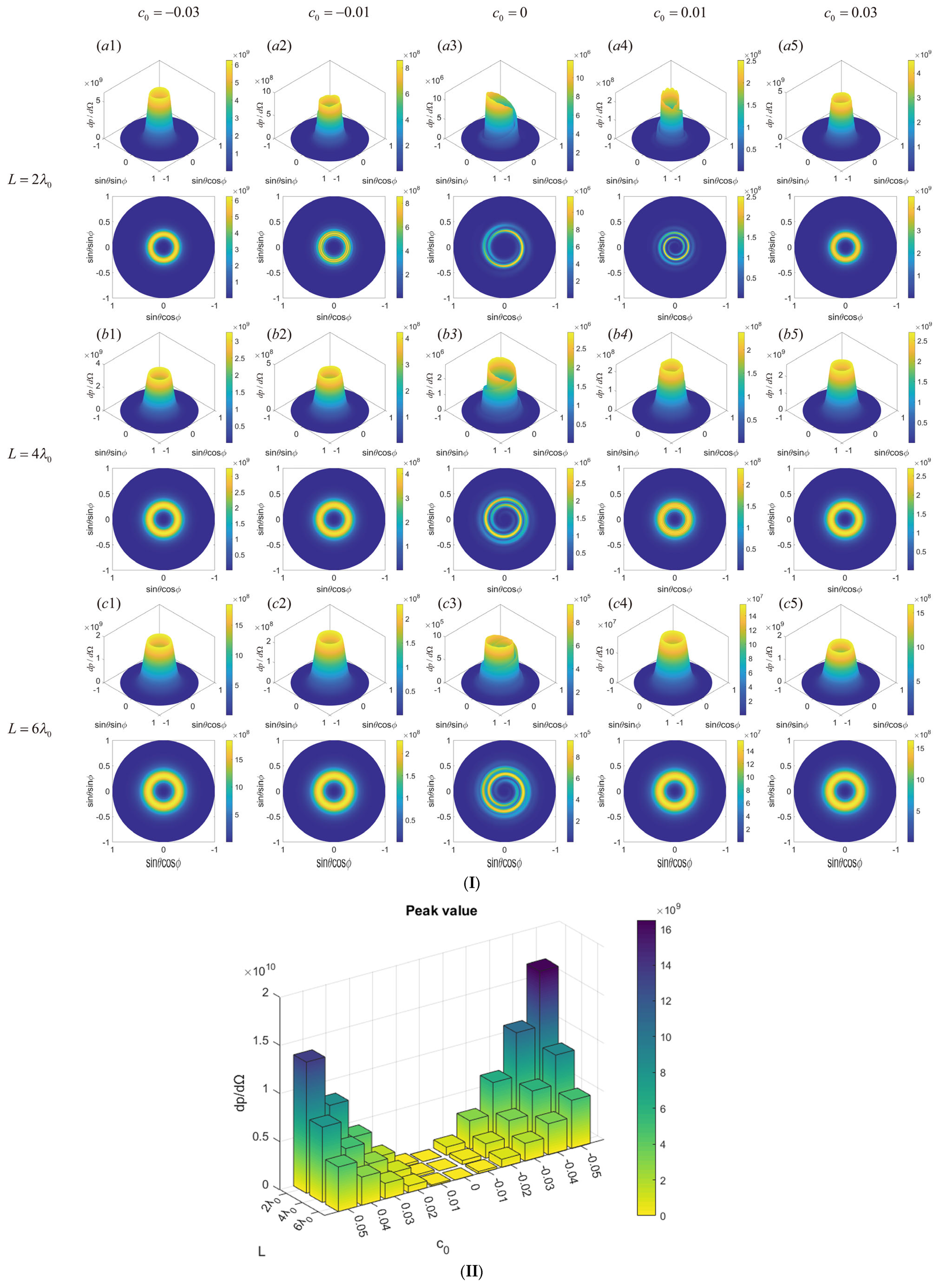
3.2. Spatial Distribution of Radiation

At the same time, the study of radiation spatial distribution in the process of electron motion also found that the chirped parameter has an effect on radiation spatial distribution. It is worth noting that we have used a cylindrical coordinate system to plot the spatial distribution of radiation, aiming to investigate the radiation behavior of electrons under the influence of the laser.

In the absence of a chirped pulse, the spatial distribution of electron radiation is affected by the pulse width. On the one hand, the radiation peak decreases with the increase in pulse width. At the same time, with the increase in pulse width, the vortex phenomenon becomes gradually obvious, and the spiral distribution tends to be closer.

When the radiation is affected by a chirped pulse, in the process of increasing the absolute value of the chirped pulse, the number of rotational layers of radiation increases, the angular gap of vortex radiation shrinks significantly, the vortex structure is rich, the spiral distribution is tighter, and the coupling phenomenon gradually begins to appear.

As the pulse width increases, the effect of the chirped parameters on vortex coupling is gradually obvious, and the effect of positive and negative chirps is different. When the pulse width is $2{\lambda }_0$, the vortex density increases obviously with the increase in the absolute value of the chirp parameter. When the chirp parameter reaches $\pm 0.03$, the vortex disappears, and the radiation distribution is circular. However, compared with Figure 3I(a2,a4), although the absolute value of the chirp is the same, the radiation distribution of the electron radiation increases significantly. However, the effect of positive and negative chirps is obviously asymmetrical, and the vortex coupling effect of negative chirps is stronger than that of positive chirps, which is similar to the motion trajectory. There is also a symmetry axis at the negative chirp, and the coupling effect of chirped parameters on space radiation is also symmetrical.

In addition, it can be seen that the morphometric transformation effect of radiation distribution is more obvious under the influence of a chirped pulse. This is because the chirped pulse causes the instantaneous frequency of the laser to change, and the electrons are subjected to higher-intensity laser action per unit of time, resulting in an increase in the energy peak of the electron radiation. At the same time, because the electrons are affected by the chirped pulse, the spiral motion frequency of the electrons increases. The spiral distribution of electron radiation tends to be tight, and the coupling occurs in the process of adjacent radiation gradually approaching, forming a circular distribution. Although the vortex phenomenon becomes more obvious when the pulse width increases, it can be seen that the coupling effect of the same chirp parameter on the spatial distribution of radiation is more obvious when the pulse width increases. Compared with Figure 3I(a4–c4), the radiation coupling of group $\left(a4\right)$ with a pulse width of $2{\lambda }_0$ occurs under the chirp of $+0.01$. The spatial distribution of radiation in group $\left(b4\right)$ with a pulse width of $4{\lambda }_0$ begins to appear as a concentric circular-like distribution, and the radiation coupling degree in group $\left(c4\right)$ with a pulse width of $6{\lambda }_0$ is extremely high—and the vortex phenomenon could not be observed.

It can be concluded that the coupling effect of chirped parameters to space radiation can be enhanced with the increase in pulse width. At the same time, it can be seen from the comparison of the time spectrum in Figure 4 that the peak value of electron radiation energy increases with the increase in the absolute value of the chirped parameter. The change in radiation energy distribution in the time dimension is also observed.

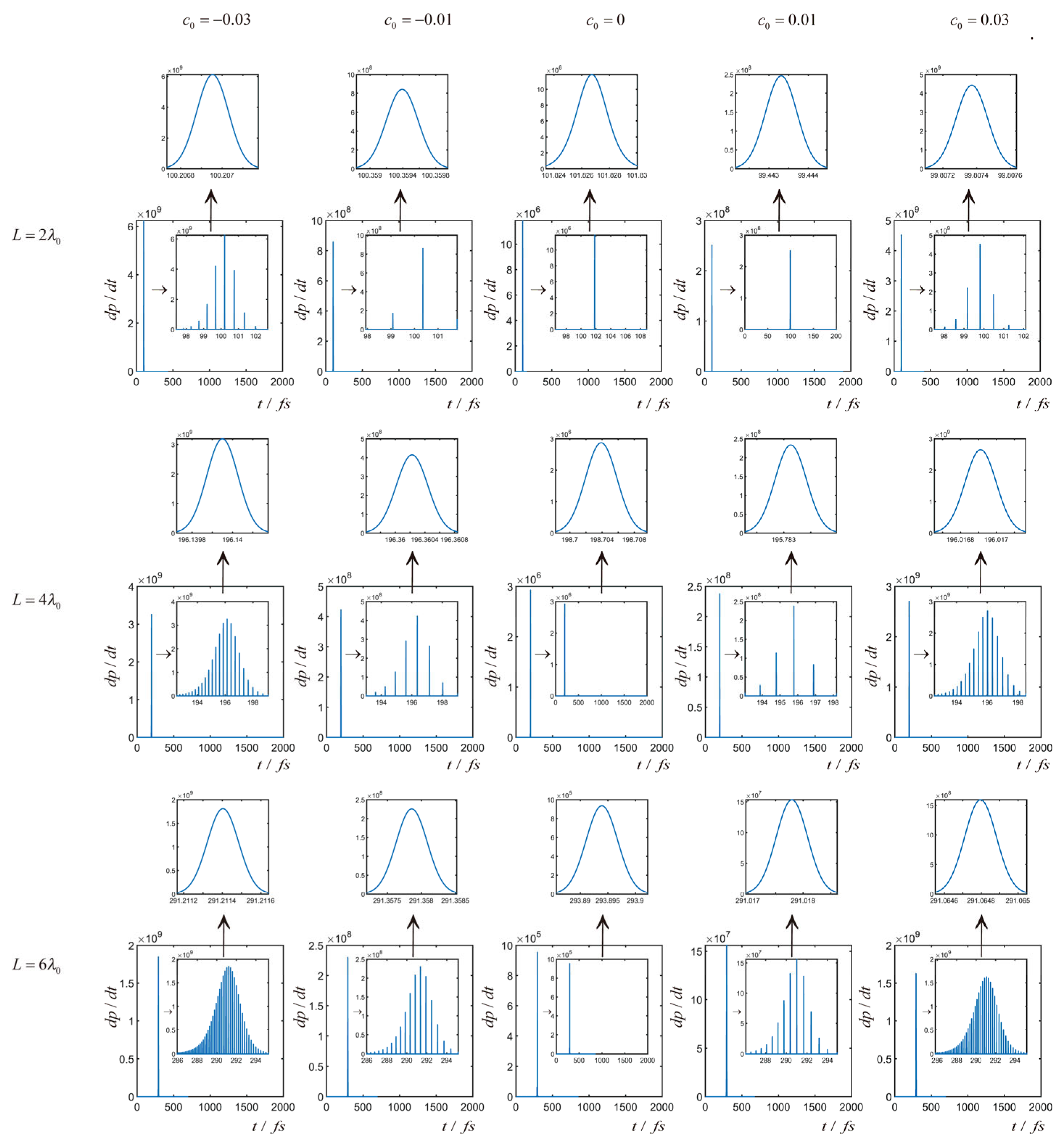
3.3. Time Spectrum Analysis

At the same time, it can be seen that the time spectrum of the chirp parameter changes under the same pulse width (Figure 4). In the process of chirp parameters changing from negative to positive, the magnitude and time of the peak power of the main peak change. The time range after the expansion of the main radiation peak is attached to the upper right corner of each complete time spectrum, from which we can observe that one of the specific manifestations of the chirp pulse on the time distribution is that the time of the peak changes under the conditions of the three groups of pulse widths.

Compared with no chirp and added chirp conditions, the peak radiation of the main peak appears earlier, but the effect of different chirp parameters is different. When the absolute value of the chirp parameter increases, it is found that the occurrence time of the main peak of the positive chirp pulse is delayed with the increase in the positive chirp value, and the occurrence time of the negative chirp pulse is advanced with the increase in the negative chirp value. Therefore, it can be seen that the occurrence time of the peak pulse of the main peak is simultaneously affected by the compound effect of the chirp and pulse width. Under certain circumstances, the combination of the chirp and pulse width may delay or advance the appearance of the main peak. Further research will be conducted on the movement of the peak pulse of the main peak. For the peak of the main peak power, with an increase in the absolute value of the chirp parameter, no matter whether the added chirp is positive or negative, the peak of the radiated power gradually increases. The main influencing factors are the change in pulse effect due to the change in the frequency and the broadening effect of chirping on the pulse.

The negative chirp means that the pulse in the high-frequency part interacts with the electron first, followed by the pulse in the low-frequency part. Therefore, the interaction between the pulse front and the electron is obvious, and the speed of electron movement to the peak is faster. At the same time, due to the action of a high-frequency pulse, the electron absorbs more energy per unit of time so that the radiation power peak appears in advance, and the peak value is greater than that of the pulse without a chirp.

The principle of positive chirping is that the frequency of the pulse front is relatively low, the wavelength is relatively long, and the wavelength is relatively short along the frequency. Therefore, the position where the energy effect is most obvious is delayed, and the time when the power peak appears is delayed. At the same time, due to the characteristics of the normal dispersive medium, the long wavelength of the front will lead to faster pulse propagation, which will cause the pulse front to move further forward, while the short wavelength part of the propagation is slow, which makes the pulse back edge more backward, resulting in the pulse broadening. This broadening gives the electrons more time to interact with the laser field, which allows them to absorb more energy, resulting in an increase in the peak power of the electrons. In addition to the change in the main peak, another obvious change is the radiation, with a relatively low amplitude appearing at different times, which is defined in this paper as the side peak. With an increase in the absolute value of the chirped parameter, the side peak appears, and the occurrence frequency increases. In the time spectrum, multiple spectral lines appear, and with an increase in the absolute value of the chirped parameter, the envelope tends to be a Gaussian-like distribution with the same main peak.

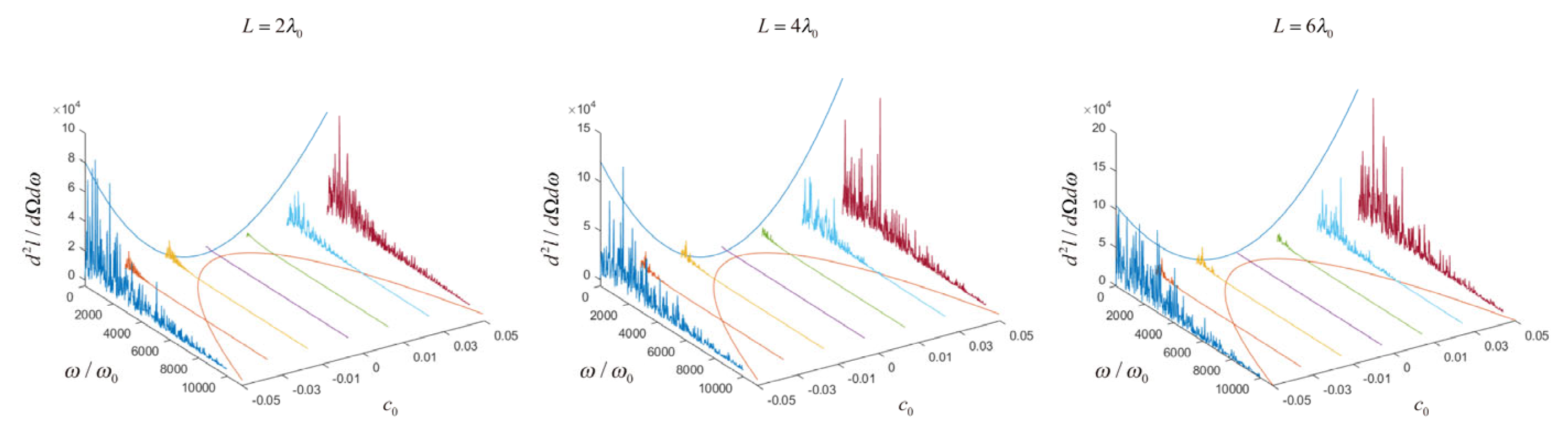
3.4. Frequency Spectrum Analysis

In addition to the change in the time dimension, the power distribution of electrons also changes significantly in the frequency domain. As shown in Figure 5, it can be seen that after adding chirped parameters, a comparison is made under the same pulse width condition, the power peak and limit frequency of the three groups of spectrums are taken out, and the envelope lines are drawn for comparison. It can be seen that the envelope lines of the radiation peak and limit frequency under the three groups of pulse width conditions show a parabolic distribution.

With the increase in the limit frequency, the frequency range of the power distribution expands, the number of sub-peaks generated at different frequencies increases, the gap between them and adjacent peaks decreases, and the power peaks in the high-frequency range become larger and larger. Under different pulse widths, the effect of the same chirp is not exactly the same, which is generally manifested as the larger the pulse width. Under the same chirped parameters, the frequency distribution tends to be uniform with an increasing frequency range. This is because under the action of a normal pulse, the frequency of the pulse is constant, so the response of the electron is also a single frequency, which will produce a sharp peak on the frequency spectrum because the chirped pulse has different frequencies at different stages of action, so the radiation frequency generated by the electron at different times and after the pulse action is different. Thus, the chirped electronic spectrum presents frequency continuity.

At the same time, because the frequency of the chirped pulse is continuously changing, the action on the electron is a continuous process, and the spectrum change generated by the response is more continuous than the mutation in the non-chirped state, so the spectrum is manifested as energy at different frequencies. At the same time, due to the addition of the chirp, the frequency of the pulse action is denser and denser, and the frequency increases in the spectrum; the larger the chirp parameter, the wider the frequency range of the pulse is, so the peak point on the spectrum becomes more, and the power peak is also generated at a larger frequency. At the same time, we observe that when the chirped parameter is added, although the total amount increases, it is still mainly distributed within the low-frequency region. With an improvement in the chirped parameter, the power distribution tends to be evenly distributed. In the range of 0–6000 Hz, when the absolute value of the chirped parameter increases, the gap between the peaks of each frequency gradually decreases.

However, the power peak of high-frequency peaks is lower than that of the low-frequency sub-peaks. Although the chirped pulse converts the equal frequency pulse into a pulse of different frequencies, the pulse action time gradually decreases as the frequency increases, and the pulse frequency changes before the electron fully interacts with the frequency pulse. Therefore, the low radiation value of high frequency is not because the energy of the high-frequency pulse itself is small but due to the result of the failure of the electron to fully interact with the pulse during the action.

4. Conclusions

In this paper, the changes in electron motion states and radiation distributions under the influence of chirped parameters and pulse width cross parameters are studied. The effect of pulse widths on chirp parameters is investigated. It is found that the compound effect of chirp parameters and a pulse width has a significant effect on t = electron trajectory and radiation characteristics, and the influence of chirp parameter changes under the same pulse width is explored. The asymmetry of the chirping effect is proposed, and the mechanism of the chirping effect is explored, which provides a theoretical basis for the parameter formulation of chirped pulse and electron interactions.

The conclusions of this paper hold significant practical application value, as they provide analytical theories for the special trajectory electrons observed in actual nonlinear Thomson scattering experiments. Additionally, this study elucidates the pulse laser parameters and underlying mechanisms responsible for the generation of such electrons, offering relevant theoretical parameters for precise electron trajectory control.

References

1. Sohbatzadeh, F.; Mirzanejhad, S.; Ghasemi, M. Electron acceleration by a chirped Gaussian laser pulse in vacuum. Phys. Plasmas 2006, 13, 123108. [Google Scholar]
2. Sun, J.; Wang, S.; Zhu, W.; Li, X.; Jiang, L. Simulation of femtosecond laser-induced periodic surface structures on fused silica by considering intrapulse and interpulse feedback. J. Appl. Phys. 2024, 136, 013103. [Google Scholar]
3. Chi, Z.; Du, Y.; Huang, W.; Tang, C. Focal spot characteristics of Thomson scattering X-ray sources. J. Appl. Phys. 2018, 124, 124901. [Google Scholar] [CrossRef]
4. Rykovanov, S.G.; Geddes, C.G.R.; Schroeder, C.B.; Esarey, E.; Leemans, W.P. Controlling the spectral shape of nonlinear Thomson scattering with proper laser chirping. Phys. Rev. Accel. Beams 2016, 19, 030701. [Google Scholar]
5. Mahreen; Prakash, G.V.; Kar, S.; Sahu, D.; Ganguli, A. Influence of pulse modulation frequency on helium RF atmospheric pressure plasma jet characteristics. Contrib. Plasma Phys. 2022, 62, e202200007. [Google Scholar] [CrossRef]
6. Aumann, S.; Donner, S.; Fischer, J.; Müller, F. Optical coherence tomography (OCT): Principle and technical realization. In High Resolution Imaging in Microscopy and Ophthalmology: New Frontiers in Biomedical Optics; Springer: Berlin/Heidelberg, Germany, 2019; pp. 59–85. [Google Scholar]
7. Galvanauskas, A. Mode-scalable fiber-based chirped pulse amplification systems. IEEE J. Sel. Top. Quantum Electron. 2001, 7, 504–517. [Google Scholar]
8. Zaouter, Y.; Guichard, F.; Daniault, L.; Hanna, M.; Morin, F.; Hönninger, C.; Mottay, E.; Druon, F.; Georges, P. Femtosecond fiber chirped-and divided-pulse amplification system. Opt. Lett. 2013, 38, 106–108. [Google Scholar] [CrossRef]
9. Yu, L.-H.; Chu, Y.-X.; Gan, Z.-B.; Liang, X.-Y.; Li, R.-X.; Xu, Z.-Z. Trends in ultrashort and ultrahigh power laser pulses based on optical parametric chirped pulse amplification. Chin. Phys. B 2015, 24, 018704. [Google Scholar]
10. Hu, Y.-H.; Wang, Y.-W.; Wen, S.-C.; Fan, D.-Y. Nonlinear images of scatterers in chirped pulsed laser beams. Chin. Phys. B 2010, 19, 114207. [Google Scholar]
11. Maher-McWilliams, C.; Douglas, P.; Barker, P.F. Laser-driven acceleration of neutral particles. Nat. Photon. 2012, 6, 386–390. [Google Scholar]
12. Singh, K.P. Electron acceleration by a chirped short intense laser pulse in vacuum. Appl. Phys. Lett. 2005, 87, 254102. [Google Scholar]
13. Wong, L.J.; Kärtner, F.X. Direct acceleration of an electron in infinite vacuum by a pulsed radially-polarized laser beam. Opt. Express 2010, 18, 25035–25051. [Google Scholar]
14. Zhang, Y.; Yang, Q.; Wang, J.; Gong, X.; Tian, Y. Zeptosecond-Yoctosecond Pulses Generated by Nonlinear Inverse Thomson Scattering: Modulation and Spatiotemporal Properties. Appl. Sci. 2024, 14, 7038. [Google Scholar] [CrossRef]
15. Hartemann, F.V.; Landahl, E.C.; Troha, A.L.; Van Meter, J.R.; Baldis, H.A.; Freeman, R.R.; Luhmann, N.C.; Song, L.; Kerman, A.K.; Yu, D.U.L. The chirped-pulse inverse free-electron laser: A high-gradient vacuum laser accelerator. Phys. Plasmas 1999, 6, 4104–4110. [Google Scholar]
16. Terzić, B.; McKaig, J.; Johnson, E.; Dharanikota, T.; Krafft, G.A. Laser chirping in inverse Compton sources at high electron beam energies and high laser intensities. Phys. Rev. Accel. Beams 2021, 24, 094401. [Google Scholar]
17. Feng, C.; Shen, L.; Zhang, M.; Wang, D.; Zhao, Z.; Xiang, D. Chirped pulse amplification in a seeded free-electron laser for generating high-power ultra-short radiation. Nucl. Instrum. Methods Phys. Res. Sect. A Accel. Spectrom. Detect. Assoc. Equip. 2013, 712, 113–119. [Google Scholar]
18. Zeng, L.; Wang, X.; Liang, Y.; Yi, H.; Zhang, W.; Yang, X. Chirped-Pulse Amplification in an Echo-Enabled Harmonic-Generation Free-Electron Laser. Appl. Sci. 2023, 13, 10292. [Google Scholar] [CrossRef]
19. Gupta, D.N.; Kumar, S.; Yoon, M.; Hur, M.S.; Suk, H. Electron acceleration by a short laser beam in the presence of a long-wavelength electromagnetic wave. J. Appl. Phys. 2007, 102, 056106. [Google Scholar]
20. Hu, Y.N.; Cheng, L.H.; Yao, Z.W.; Zhang, X.B.; Zhang, A.X.; Xue, J.K. Direct electron acceleration by chirped laser pulse in a cylindrical plasma channel. Chin. Phys. B 2020, 29, 084103. [Google Scholar]
21. Fang, T.; Liang-You, P.; Qi-Huang, G. Ionization of atoms by chirped attosecond pulses. Chin. Phys. B 2009, 18, 4807–4814. [Google Scholar]
22. Jie, W.; Zhen, Z.; Xue-Shen, L. Extension of high-order harmonics and generation of an isolated attosecond pulse in the chirped laser field. Chin. Phys. B 2010, 19, 093201. [Google Scholar]
23. Wang, H.-L.; Yang, A.-J.; Leng, Y.-X.; Wang, C.; Xu, Z.-Z.; Hou, L.-T. Optical parametric chirped pulse amplification based on photonic crystal fibre. Chin. Phys. B 2011, 20, 084208. [Google Scholar]
24. Jisrawi, N.M.; Galow, B.J.; Salamin, Y.I. Simulation of the relativistic electron dynamics and acceleration in a linearly-chirped laser pulse. Laser Part. Beams 2014, 32, 671–680. [Google Scholar]
25. Li, J.-X.; Zang, W.-P.; Tian, J.-G. Electron acceleration in vacuum induced by a tightly focused chirped laser pulse. Appl. Phys. Lett. 2010, 96, 031103. [Google Scholar]
26. Kumar, S.; Yoon, M. Electron acceleration by a chirped circularly polarized laser pulse in vacuum in the presence of a planar magnetic wiggler. Phys. Scr. 2008, 77, 025404. [Google Scholar]
27. Koga, J.; Esirkepov, T.Z.; Bulanov, S.V. Nonlinear Thomson scattering in the strong radiation damping regime. Phys. Plasmas 2005, 12, 093106. [Google Scholar]
28. Lee, K.; Chung, S.Y.; Kim, D.E. Relativistic Nonlinear Thomson Scattering: Toward Intense Attosecond Pulse. In Advances in Solid State Lasers Development and Applications; IntechOpen: London, UK, 2010. [Google Scholar]
29. Glushkov, A.V. Multiphoton spectroscopy of atoms and nuclei in a laser field: Relativistic energy approach and radiation atomic lines moments method. In Advances in Quantum Chemistry; Academic Press: New York, NY, USA, 2019; Volume 78, pp. 253–285. [Google Scholar]
30. Wang, Y.; Yang, Q.; Chang, Y.; Lin, Z.; Tian, Y. Collision off-axis position dependence of relativistic nonlinear Thomson inverse scattering of an excited electron in a tightly focused circular polarized laser pulse. Chin. Phys. B 2023, 33, 013301. [Google Scholar]
31. Barton, J.P.; Alexander, D.R.; Barton, J.P.; Alexander, D.R. Fifth-order corrected electromagnetic field components for a fundamental Gaussian beam. J. Appl. Phys. 1989, 66, 2800–2802. [Google Scholar]
32. Salamin, Y.I.; Keitel, C.H. Electron acceleration by a tightly focused laser beam. Phys. Rev. Lett. 2002, 88, 095005. [Google Scholar]
33. Zhang, S.Y. Accurate correction field of circularly polarized laser and its acceleration effect. J. At. Mol. Sci. 2010, 1, 308–317. [Google Scholar]
34. Greiner, W. Classical Electrodynamics. John Wiley & Sons: Hoboken, NJ, USA, 2021. [Google Scholar]
35. Shampine, L.F.; Watts, H.A. Practical Solution of Ordinary Differential Equations by Runge—Kutta Methods [Writing a High-Quality Code Description of RKF45, in FORTRAN for CDC 6600 Computer]; No. SAND-76-0585; Sandia Labs.: Albuquerque, NM, USA, 1976. [Google Scholar]
36. Nishidate, Y. A Ray Equation for Optically Anisotropic Inhomogeneous Media and Its Closed-Form Solutions for Estimating Ray-Trajectories. Available online: https://www.researchgate.net/publication/298887528_A_ray_equation_for_optically_anisotropic_inhomogeneous_media_and_its_closed-form_solutions_for_estimating_ray-trajectories (accessed on 13 January 2025).
Figure 1. Diagram of chirped pulse and electron interaction process.
Applsci 15 03619 g001
Figure 2. (I). Comparison of the electron motion tracks with different pulse widths under different chirp parameters: the pulse width L is taken as three sets of values, group (a) corresponds to 2 λ 0 , group (b) corresponds to 4 λ 0 , and group (c) corresponds to 6 λ 0 . The corresponding pulse durations are 6.7 f s ,     13.3 f s ,   a n d   20   f s , All the different trajectory colors represent different chirp parameters. The colors of the motion trajectories under different chirped parameters are marked in the upper right corner of the figure. (II). Expansion diagram of the electron motion trajectory with different pulse widths under different chirped parameters.
Applsci 15 03619 g002aApplsci 15 03619 g002b
Figure 3. (I). Front view and top view of the spatial distribution of electronic radiation, group (a) corresponds to 2 λ 0 , group (b) corresponds to 4 λ 0 , and group (c) corresponds to 6 λ 0 . (II). Histogram of the peak value of the spatial distribution of electron radiation under different parameters. Each point is the logarithm of the peak value of the spatial distribution of radiation under different pulse widths and chirp parameters with a base of 10 for comparison.
Applsci 15 03619 g003
Figure 4. Time spectrum, complete spectral line, and peak spread spectral line of the peak of the electron radiated power.
Applsci 15 03619 g004
Figure 5. Comparison of the frequency spectrum of the peak electron radiated power under three pulse widths. The chirp parameters c 0 from (left) to (right), respectively, are 0.05 , 0.03 , 0.01 ,   0 ,   0.01 ,   0.03 ,   a n d   0.05 .
Applsci 15 03619 g005
Disclaimer/Publisher’s Note: The statements, opinions and data contained in all publications are solely those of the individual author(s) and contributor(s) and not of MDPI and/or the editor(s). MDPI and/or the editor(s) disclaim responsibility for any injury to people or property resulting from any ideas, methods, instructions or products referred to in the content.