Featured Application
The results offer the possibility to better understand the main factors for the prediction of the site effect for the seismic analysis and design of infrastructures. They could also help enhance the codes’ provisions in this regard. The methodology offers an insight into further possibilities for the integration of artificial intelligence within the domain of structural and geotechnical engineering.
Abstract
The identification of the most pertinent site parameters to classify soils in terms of their amplification of seismic ground motions is still of prime interest to earthquake engineering and codes. This study investigates many options for improving soil classifications in order to reduce the deviation between “exact” predictions using wave propagation and the method used in seismic codes based on amplification (site) factors. To this end, an exhaustive parametric study is carried out to obtain nonlinear responses of sets of 324 clay and sand columns and to constitute the database for neuronal network methods used to predict the regression equations of the amplification factors in terms of seismic and site parameters. A wide variety of parameters and their combinations are considered in the study, namely, soil depth, shear wave velocity, the stiffness of the underlaying bedrock, and the intensity and frequency content of the seismic excitation. A database of AFs for 324 nonlinear soil profiles of sand and clay under multiple records with different intensities and frequency contents is obtained by wave propagation, where soil nonlinearity is accounted for through the equivalent linear model and an iterative procedure. Then, a Generalized Regression Neural Network (GRNN) is used on the obtained database to determine the most significant parameters affecting the AFs. A second neural network, the Radial Basis Function (RBF) network, is used to develop simple and practical prediction equations. Both the whole period range and specific short-, mid-, and long-period ranges associated with the AFs, Fa, Fv, and Fl, respectively, are considered. The results indicate that the amplification factor of an arbitrary soil profile can be satisfactorily approximated with a limited number of sites and the seismic record parameters (two to six). The best parameter pair is (PGA; resonance frequency, f0), which leads to a standard deviation reduction of at least 65%. For improved performance, we propose the practical triplet with Vs30 being the average shear wave velocity within the upper 30 m of soil below the foundation. Most other relevant results include the fact that the AFs for long periods (Fl) can be significantly higher than those for short or mid periods for soft soils. Finally, it is recommended to further refine this study by including additional soil parameters such as spatial configuration and by adopting more refined soil models.
1. Introduction
Local site conditions play a crucial role in determining the level of damage experienced during earthquakes, as demonstrated from past experiences in the Mexico City (1985), Loma Prieta (1989), Northridge (1994), Kobe (1995), and, more recently, Turkey (2023) earthquakes. In many cases, the geological and geotechnical characteristics of an area can amplify seismic waves, leading to greater ground shaking and structural damage. Soil type, liquefaction conditions, site topography, building design, and historical context are some of the key factors affecting the severity of shaking and damage [1,2,3,4,5,6,7,8,9]. Addressing these factors through better engineering practices and building codes can mitigate damage in future events. To this end, for many decades, using local elastic response spectra based on soil categorization and seismic hazard has been the common way to evaluate seismic input for the design and evaluation of structures. Soil categorization and characterization are also crucial when applying Ground Motion Prediction Equations (GMPEs) for accurate predictions of local ground motion and/or for developing site-specific spectra while taking into account local site conditions.
Numerous researchers have put forward different site parameters to classify and characterize soils. Borcherdt (1994) was among the first to recommend using the average shear wave velocity over the upper 30 m (Vs30) as a fundamental criterion for soil characterization [10]. This parameter has since gained widespread acceptance in seismic assessments. However, there are concerns about Vs30’s effectiveness in adequately representing site effects on its own [11,12,13,14,15,16,17,18,19,20]. More recent GMPEs that utilize various databases continue to rely on Vs30 to characterize site conditions [21,22,23,24]. However, Vs30 is frequently complemented or replaced by other site parameters, including the fundamental frequency, f0, the average shear wave velocity at different depths within the soil profile, or the depth to hard bedrock [19,22,25,26,27,28,29]. Recent and current regulatory codes use peak ground acceleration (PGA) or spectral values for reference soil, along with Vs30, to modify the design spectra’s characteristics—specifically the plateau bandwidth, level, and long-period decay—to suit local site conditions. These regulations focus on the free surface response to ascending waves, which governs how seismic waves interact with structures. This methodology is fundamental to major international building codes, including the 1997 NEHRP Provisions, the 1997 Uniform Building Code, Eurocode 8 (ENV 1998), the International Building Code (IBC 2012), and the National Building Code of Canada (NBC) (2015a, b, 2020) [29,30,31,32,33,34]. Recent studies have incorporated multiple soil parameters using Generalized Regression Neural Network models. These models are founded on the wave propagation theory applied to linear viscoelastic soil profiles sourced from the Japanese Kiban Kyoshin Network (KiK-net) and the US Geological Survey (USGS) [7,35].
Site amplification is usually captured by relying on only few straightforward site proxies’ values (like Vs30 and contrast velocity). However, this simplification can lead to various challenges, including Vs30’s inability to reflect the shear wave velocity profile across the entire soil depth, which can result in a skewed seismic response for short, mid, and/or long periods. Given the complex nature of the problem, the selected limited set of site proxies used to predict site amplification may not necessarily be the best combination, especially because the literature lacks a systematic evaluation of the performance of a limited number of different site proxy combinations.
On the other hand, artificial neural networks (ANNs) are particularly effective for prediction tasks due to their capacity to model complex nonlinear relationships within high-dimensional datasets. They perform well across various applications, such as time series forecasting and image recognition. Additionally, techniques like regularization and optimization enhance their performance, improving accuracy and reducing the risk of overfitting. Overall, neural networks are powerful tools for generating reliable predictions in many fields [36,37,38,39,40,41,42,43]. Consequently, the use of ANNs to identify the most prominent selections of site proxies and how they correlate to site amplification factors offers a recent perspective that can help fill the existing gap.
This study aims to identify the most effective site parameters for predicting the site amplification of the seismic response at the free surface of a soil deposit. More specifically, it focuses on establishing relationships between the amplification factor of the spectral response and a limited set of site proxies that describe the characteristics of soil profiles based on predictions of selected ANN methods.
To achieve this goal, this study examines the 1D nonlinear responses of monolayer soil profiles with varying thicknesses and shear wave velocities, situated above a semi-infinite bedrock layer, subject to different seismic records, with varying intensities and frequency contents. More specifically, a total of 324 soil profiles of sand and clay are analyzed, each represented by a single layer with depths varying from 5 to 200 m and a shear wave velocity ranging from 100 to 600 m/s, underlain by a bedrock layer with a shear wave velocity varying between 750 and 1500 m/s. The nonlinear site responses of these profiles to the vertical propagation of shear (S) waves are calculated, including responses at free surfaces, which are used to determine site amplification factors. Fourteen (14) input waveforms are selected based on the recent studies by Boudghene Stambouli et al. (2017) and Dif and Boudghene Stambouli (2023) [8,35]. Each of the considered profiles is subjected to these fourteen input motions, normalized to eleven different PGA levels: 0.01, 0.05, 0.1, 0.2, 0.3, 0.4, 0.5, 0.6, 0.75, 0.9, and 1.05 g. This approach allows for the calculation of the mean amplification for each PGA value, covering all relevant seismic frequency ranges. In total, 3564 geometric average amplification factors for each soil type are derived (324 soil profiles × 11 PGAs).
Several methods exist to calculate ground response with nonlinear behaviour. Nonlinear time history analyses are the common method for investigating the dynamic nonlinear behaviour of structures but are less widely used for soils. They are typically conducted using models discretizing the space domain, such as finite element models. While these methods generally yield accurate results and can model complex problems, they can be time-consuming due to their step-by-step integration procedure in the time domain combined with the iterative process for achieving a direct representation of the nonlinear soil response [44]. Instead, engineers often resort to a viscoelastic equivalent linear model combined with an iterative process, called equivalent linear analysis, to obtain the nonlinear solution for soils. This method, which is typically more computationally efficient, yields satisfactory results for engineering applications, especially within the relevant frequency range and for simple and smooth nonlinear behaviour [44,45,46,47,48,49]. Johari and Momeni (2015) have shown that nonlinear calculations of soil responses provided only slight performance improvements over equivalent linear methods while demanding considerably more time and complexity [47]. Consequently, given the large number of analyses to carry out (about 100,000), the equivalent linear approach is adopted in this study for efficiency.
Furthermore, numerical methods, based on the finite element method, can solve one-, two-, and three-dimensional nonlinear soil problems, where amplifications can differ significantly from 1D scenarios, especially in the presence of valleys or rugged topography. The effects of such geometric and topographic parameters had been considered in previous studies, such as those of Paolucci and Morstabilini (2006) and Boudghene Stambouli et al. (2018) [50,51]. However, such specific site effects are beyond the scope of this study, and they are not included in basic code specifications. Consequently, for the sake of efficiency, simplification, and direct comparison with codes and the main body of literature, 1D modelling of soil and wave propagation is considered in this study. Furthermore, this avenue offers the possibility of obtaining a simple analytical solution to the wave propagation problem.
Soil nonlinearity is incorporated using shear modulus degradation curves that show the variations in shear modulus (G) with respect to shear strain (γ) levels and loading history (cycling), as detailed hereafter. Shear modulus degradation under cyclic loading has been studied by several researchers using resonant column or enhanced triaxial tests. Seed and Idriss (1970) were pioneers in developing and widely applying shear modulus reduction and damping curves specifically for sand [52]. In 1991, Vucetic and Dobry introduced the plasticity index (IP) to define shear modulus degradation curves for clay [53,54]. In 1993, Ishibashi and Zhang added another parameter, the effective confining pressure, used alongside the IP to better capture the behaviour of soils with low plasticity indices [55]. That same year, the Electric Power Research Institute (EPRI) created its own soil degradation curves by combining shear modulus reduction and damping curves, allowing for broader applicability across cohesionless soils, from gravelly sands to low plasticity silts and sandy clays [56]. More recently, Darendeli (2001) proposed a new set of degradation curves, indicating that the degree of linearity increases with the plasticity index (IP), mean effective stress, and overconsolidation ratio (OCR) [57]. Such a model, while considered more appropriate for representing soil nonlinearity, requires a set of additional soil parameters to those used in our study which will extend the number of required nonlinear analyses. In order to streamline our analysis, limit the number of analyses, and focus on identifying effective proxies for soil profiles, we selected simpler degradation models proposed by Sun et al. (1988) [58] for clay and by Seed and Idriss (1970) [52] for sand. These models require minimal soil properties while still representing the nonlinear behaviour of soils under cyclic loading accurately enough [52,58]. Additionally, we incorporate the damping curves from the study by Idriss (1990), which provide insights into how damping ratios vary with strain levels [59]. This combination allows us to simplify our approach while retaining the critical features for predicting the seismic response of clay and sand, which ultimately should facilitate the identification of the most suitable proxies for soil characterization in seismic assessments.
To explore the correlation between the average amplification factor and various sets of soil characteristics, we use an artificial neural network (ANN) approach. This method effectively captures complex relationships and nonlinear interactions among input variables. To enhance our analysis, a sensitivity analysis is conducted using the neural network model. This analysis aims to identify which soil characteristics serve as the best site proxies for predicting the amplification factor. By examining how changes in these variables (proxies) impact the output, we can pinpoint the most influential parameters, thereby improving our understanding of soil behaviour in seismic contexts and facilitating better site characterization in future studies.
2. Derivation of Amplification Factors (AFs)
2.1. Introduction
For a given signal, the amplification factor at given period (T), in terms of spectral acceleration, can be expressed as the ratio of the response spectrum at the surface to the response spectrum at the outcropping reference rock as follows:
where and are the 5% response acceleration spectra at the free surface and at the reference rock (bedrock), respectively, while T is the period of the structure.
Because the response of soils under strong excitations is nonlinear by nature, and in order to apply the theory of wave propagation in an elastic medium, the problem needs to be linearized. The equivalent linear method, first introduced by Jacobson (1930) [60] and extended by Hudson (1965) [61] and Seed and Idriss (1970), is largely used in nonlinear problems of soils and structures [49,52]. This method replaces the nonlinear behaviour with an equivalent linear spring in parallel with a viscoelastic damper to include the stiffness and damping associated with the hysteresis of the soil or structure. However, given the nonlinear nature of the problem, the stiffness and damping vary with the displacement or deformation level, which is unknown. Consequently, this linearization method adopts an iterative scheme in order to converge at the target displacement, typically the maximum or design displacement. For a wave propagation problem, therefore, the shear modulus (G) and the damping ratio (ξ), which are functions of the deformation level in the middle of each layer, are adjusted at each iteration in order to capture the hysteresis of the soil at the target deformation level. A wave equation can be used to solve the shear wave propagation in soils [62,63,64,65,66]. Schnabel et al. (1972) proposed an algorithm based on the continuous solution of the wave equation, the main steps of which are summarized in the Supplementary File, section (a) [67,68].
2.2. Input Waveforms
This section discusses and describes the selected input accelerograms, b(t), used in the above algorithm for the calculation of the amplification factors in this study.
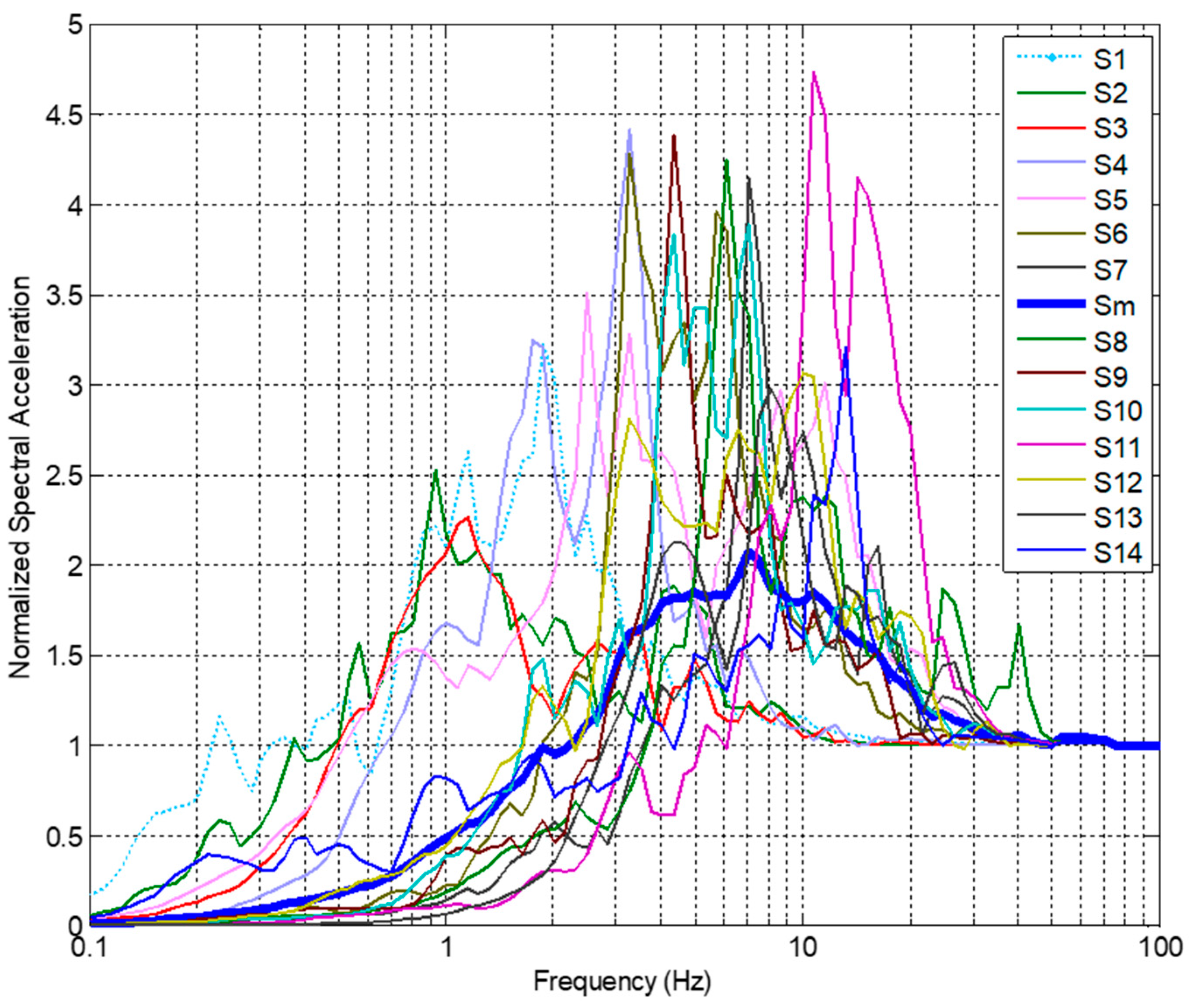
From the RESORCE database [69], sets of 14 input waveforms (S1 to S14), recorded on outcropping rock, are selected for this study, and their characteristics are listed in the Supplementary File, section (b). The selected accelerograms are drawn from real earthquakes and satisfy certain conditions to ensure a representative average amplification factor that is not biassed by a spectral content that is too rich in either short, medium, or long frequency [35]. The main characteristics of the 14 reference acceleration time histories are summarized in the Supplementary File. Figure 1 presents the spectra of the selected signals normalized to a PGA of 1 g. Each normalized seismic signal is scaled by the appropriate factor to achieve the chosen eleven PGA values (0.01 g, 0.05 g, 0.1 g, to 0.9 g, with a step of 0.1 g and 1.05 g). We then compute 49 896 time-history seismic responses (14 records × 11 PGA levels × 324 soil profiles) using the shear modulus degradation curve of the clay, and the same process and number of seismic responses are also carried out for sand.
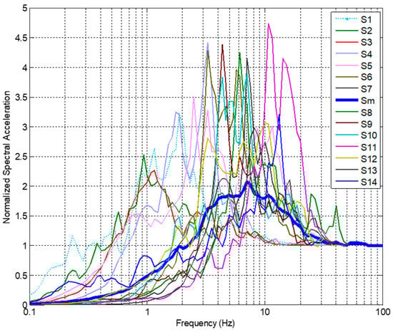
Figure 1.
Normalized (to PGA = 1 g) acceleration spectra of signals used.
2.3. Site Model, Wave Propagation Solution, and Transfer Function T(f)
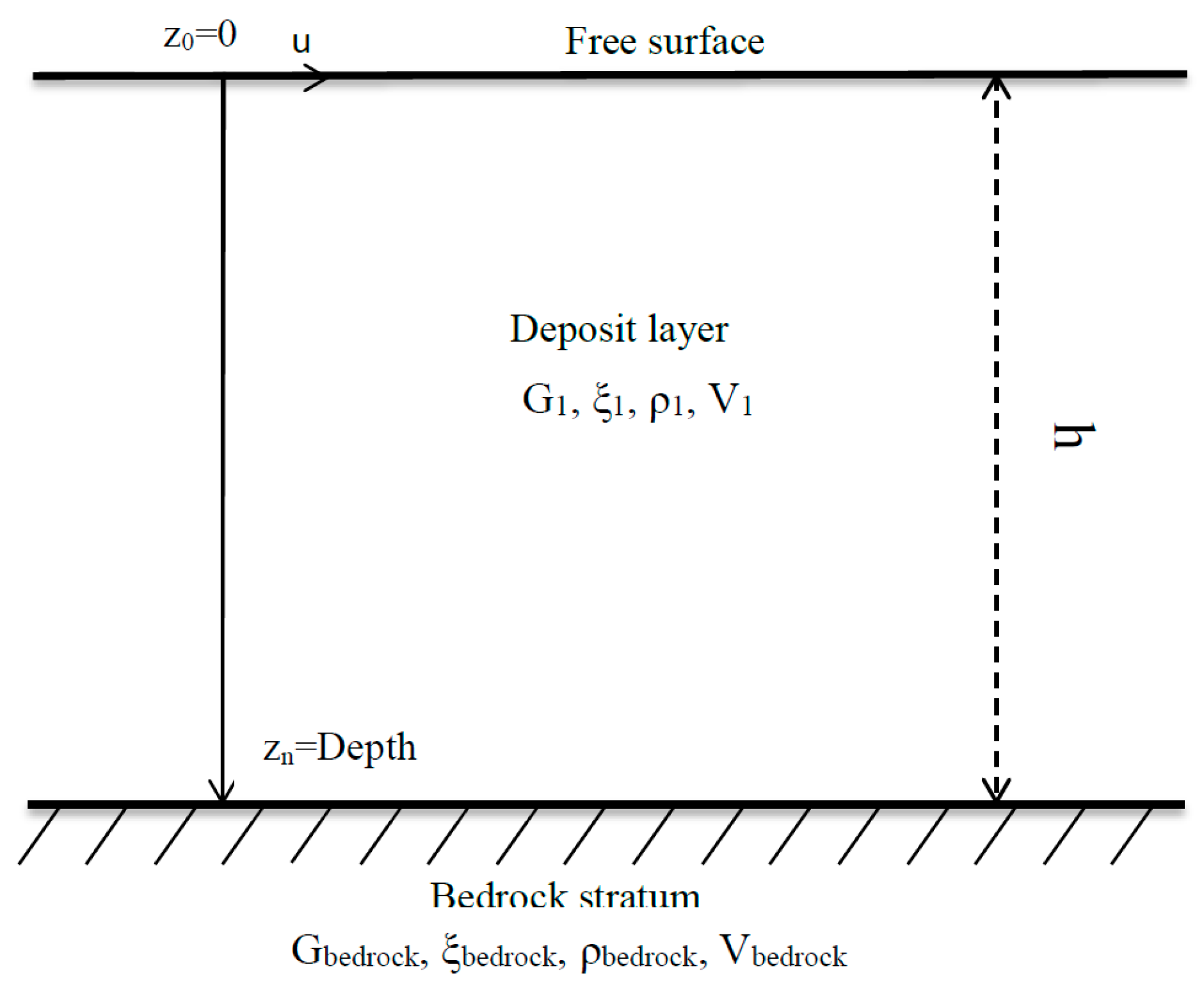
In this study, the soil is idealized by one horizontally layered soil deposit resting on a bedrock substratum (see Figure 2).
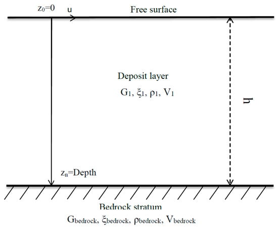
Figure 2.
A schematic representation of the 1D site response.
The layer is fully defined by its shear modulus, G, or shear wave velocity, V; thickness, h; damping ratio ζ; and mass density ρ. The underlying half-space has shear wave velocity Vbedrock. The vertical z-axis is oriented downwards. The response of the soil column to harmonic, vertically incident plane shear waves is governed by differential Equation (2) [68]:
where ui is the horizontal displacement in the ith layer (in this study, i = 1 for the monolayer soil deposit).
- with:
The general solution of governing differential Equation (2) is a summation of up-going and down-going plane waves with unknown amplitudes, Ai and Bi, for each layer, given in Equation (4).
The transfer function is a complex function defined as the ratio of the layer surface amplitude to the layer bottom amplitude, and the procedure to drive such a function can be found in the classical literature [68,70,71]. For a single layer of soil, it can be written, using Euler’s Law, as follows:
where is a complex wave number, defined as
and is the complex impedance ratio, defined as
where is the damping ratio in the bedrock, which generally has a negligible effect on the results, and is taken as null in this study.
For a particular soil profile, AF(T) is computed once the transfer function T(f) is known using the equivalent linear model procedure extensively described in the geotechnical earthquake engineering literature [35,67,68].
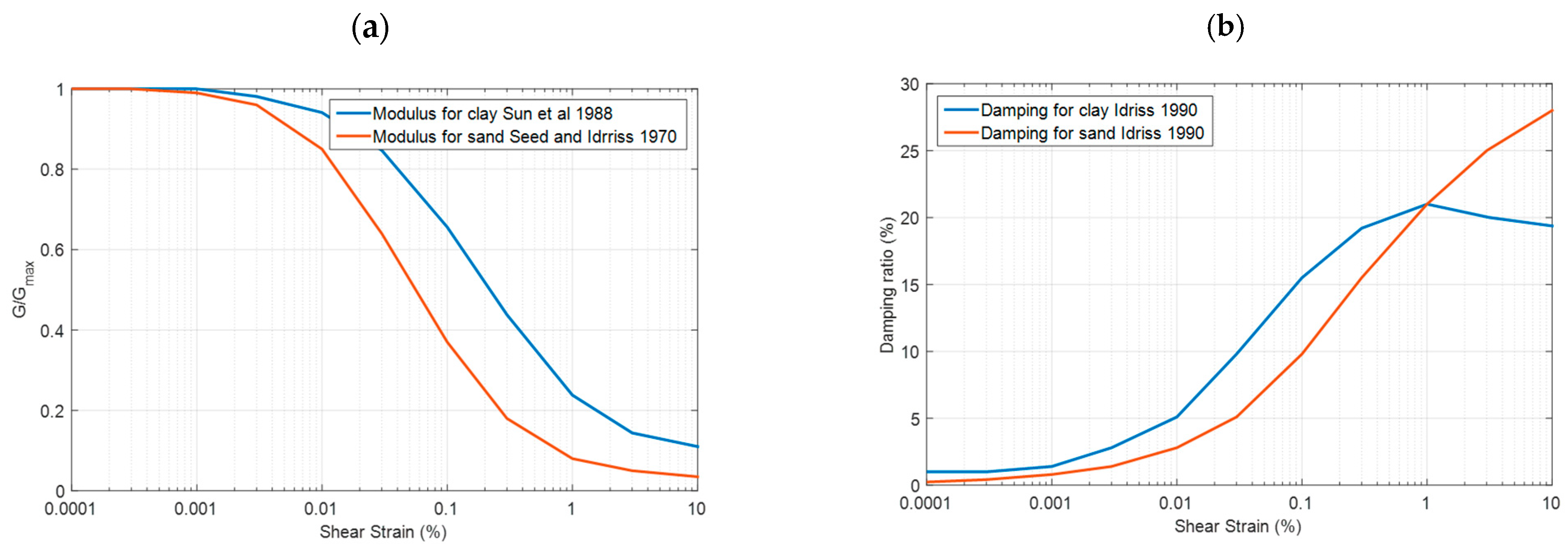
As mentioned earlier, we used the simple shear modulus degradation model proposed by Sun et al. (1988) [58] for clay and the model proposed by Seed and Idriss (1970) [52] for sand (G/Gmax is a function of the shear strain). For damping variation with shear strain, the curves of Idriss (1990) are used for both clay and sand [59]. These selected models are illustrated in Figure 3, and their key parameter values are presented in Supplementary File, section (c).
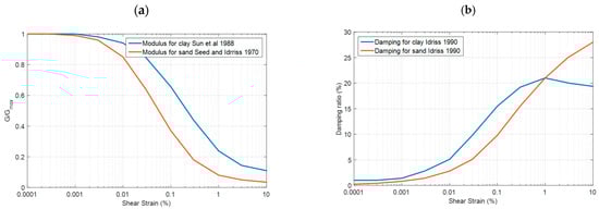
Figure 3.
Degradation curves for clay and sand. (a) Shear modules. (b) Damping ratios. Refs. [52,58,59].
Based on these models, the equivalent shear modulus and damping ratio are obtained by an iterative process to ensure that the values used are consistent with the strain level obtained according to the procedure described above. At the interface of adjacent layers, the stress and displacement continuity equations are solved, and the relationships between these amplitudes for two adjacent layers are established. Afterward, the waves are propagated from the bottom (unit up-going amplitude) to the top layer using the free surface condition (shear stress = 0). The wave amplitudes and the transfer function can be derived with respect to the motion at the outcropping bedrock.
2.4. Database
2.4.1. Descriptions of Soil Profiles Studied
In this study, a monolayer soil profile is characterized by one of six different shear wave velocity values, 100, 150, 200, 300, 400, and 600 m/s, which overcomes a semi-infinite bedrock. The latter, for its part, is characterized by a shear wave velocity equal to 750, 800, 900, 1000, 1200, or 1500 m/s. The depth of the soil layer varies from 5 to 10, 20, 30, 50, 75, 100, 150, and 200 m. In total, three hundred twenty-four (324) soil profiles are generated and considered for this study. Furthermore, all 324 soil profiles are considered in two sets of profiles for a total of 648 different soil conditions: 1—clay/cohesive soil; 2—sand/granular soil. Although certain rare exceptions may exist, the considered variants of simplistic soil profiles thus generated by the aforementioned combinations cover virtually all practical cases encountered in nature and in engineering practice.
2.4.2. Selection of Site Parameters Studied
Each soil profile can be partially described by a few site parameters. In this paper, we investigate seven of them. Extensive studies of seismic site response have been performed in recent decades. In 1994, Borcherdt developed intensity-dependent, short- and long-period amplification factors based on the average shear wave velocity measured over the upper 30 m of a site [10]. Seed et al. (1988) developed a geotechnical site classification system based on the shear wave velocity, the depth to bedrock, and general geotechnical descriptions of soil deposits [72]. Seed et al. (1991) [73] then developed intensity-dependent site amplification factors that modify the baseline “rock” peak ground acceleration (PGA) to account for site effects. With such a site, PGA value, and site-dependent normalized acceleration response spectra, Martin and Dobry (1994) derived site-dependent design spectra (primarily based on the site classification system and amplification factors) [11], which were incorporated in the 1997 Uniform Building Code (UBC) [30]. The National Building Code of Canada (NBC) (2005, 2015a, b) and a later version (2020) adopt the same philosophy as the UBC, where the soil classification as well as site design spectra are based on the shear wave velocity in the upper 30 m supporting the foundations [32,33,34]. However, two important limitations are associated with such an approach.
First, it requires a relatively extensive field investigation, and second, it overlooks the potential importance of other site parameters, such as the fundamental frequency or depth to bedrock, among others, which have been identified by many researchers as pertinent for site classification [26,27,28,35,74].
To overcome the above limitation, our study considers the following parameters in addition to the Vs30: the depth of deposit to bedrock (depth); the average shear velocity () over that depth; the velocity contrast, that is, the ratio between the shear wave velocity in the bedrock and at the surface (Cv); the second velocity contrast, that is, the ratio between the shear wave velocity in the bedrock and the average shear wave velocity over the upper 30 m (Cv2); the soil profile’s fundamental frequency (); and the PGA in the bedrock. The inclusion of the PGA as a parameter of the study is justified by the well-established fact that site amplification for nonlinear soil is fundamentally dependent on the intensity of the input wave. The site proxies considered are calculated using Relations (8) to (13) as follows:
which is the thickness of the first layer (deposit layer), h1, with the bedrock being considered as a half-infinite space (see Figure 2).
where is the shear wave velocity in the first (deposit) layer:
where l30 is the number of distinct layers found in the top 30 m:
The fundamental soil frequency f0 is determined by using the simplified Rayleigh procedure, described by Dobry et al. (1976) [75], based on Equations (13) and (14):
where is the depth of the midpoint of layer (i), and the values correspond to the estimated deformations due to the fundamental mode shape at the top of each layer (i), derived according to Dobry et al. (1976) as follows [75]:
To better illustrate the domain of validity of this study, the covered site parameters domain is summarized in Table 1 through 10%, 50%, and 90% fractiles for all site parameters.

Table 1.
The 10%, 50%, and 90% fractiles of the studied parameters.
2.4.3. Correlation Between Site Parameters
All the parameters considered are not fully independent, as shown by the coefficient of determination (R2) presented in Table 2, calculated for each pair of parameters for all soil profiles considered. There exist strong correlations between the pairs (Cv, Cv2), (Vsm, Cv), (Vsm, Vs30), (Vs30, Cv), and (Vs30, Cv2), as indicated by the coefficients of determination (R2) generally exceeding 0.62. However, very weak correlations, notably for the pairs (Cv, Depth) and (Vsm, Depth), and weak correlations for the pairs (Cv, f0), (f0, Vsm), and (Depth, Vs30), with the R2 value ranging between 0.25 and 0.37, are observed. Finally, a mitigated correlation, with R2 = 0.51, is observed for the couple (f0, Depth). These correlation indicators are useful for selecting independent site parameters for the models relating site amplification to site characteristics.
Table 2.
Correlations (R2) between various site parameters.
3. Computed Amplification Factors: Main Statistical Characteristics
3.1. Validation of Adopted Methodology for Computation of AFs
Earlier studies confirmed that the equivalent linear method combined with the wave propagation solution in the frequency domain, as adopted in this study, instead of the nonlinear time history analysis demanding much more computational effort, typically yields satisfactory results for engineering applications [47]. Many examples of the validation of this approach are documented in DEEPSOIL [70]. Furthermore, using the DEEPSOIL 7.0 software, we carry out a nonlinear time history analysis on a specific site among the soil profiles used in this study (a deposit of 5 m in depth with a shear wave velocity of 300 m/s on a bedrock with a shear velocity of 800/s), submitted to the Kobe (1995) record (PGA = 0.82 g). The results are compared to those obtained using DEEPSOIL with the equivalent linear model, and practically identical free surface response time histories and free surface response acceleration spectra are obtained. A difference of 0.005, less than 0.2%, is observed in the amplification factor.
For more flexibility, ease of automation, and to efficiently carry out the parametric study, the above procedure is implemented in Matlab R2023a© and used to compute the ground time-history responses. To validate the developed code, the results are carefully and successfully checked for many validation examples against those provided by other codes, namely, DEEPSOIL [70] and EERA [71]. A relative difference of less than 0.3% is obtained in terms of the maximum acceleration at the free surface.
3.2. General Background of Computed AFs
This section presents on overview of the computed sets of frequency-dependent AFs and their short- to mid- and long-period average values. These data are essential and constitute the learning set needed to identify the key parameters controlling the site response characteristics.
In total, 99,792 AF(T) curves are computed using (Equation (1)) for the 324 soil profiles under the 14 seismic excitations normalized by 11 PGA levels for the two types of soils (clay and sand). The AF curves for clay are shown in Figure 4, and those for sand are shown in Figure 5. They may be written in the general form of , where
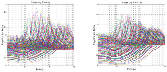
Figure 4.
Average amplification factors for 324 sets of clay soil profiles at 0.1 g and 0.75 g PGA levels.
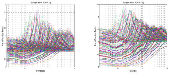
Figure 5.
Average amplification factors for 324 sets of sand soil profiles at 0.1 g and 0.75 g PGA levels.
- is introduced to identify the soil profile, ;
- for clay (using the shear modulus degradation curve of clay) and for sand (using the shear modulus degradation curve of sand);
- , is the ith structural period, and AF values are systematically computed for 100 values, equally spaced between 0.01 and 10 s on a logarithmic period axis;
- , for the identification of the PGA level, and lo, vary from 1 (for PGA = 0.01 g) to 11 (for PGA = 1.05 g).
For instance, stands for the AF obtained at the soil profile P20 of clay type, subjected to the eighth seismic excitation, , for the 50th period (T = Log−1 (−2 + (50 − 1) × (Log 10 − Log (0.01)) = 0.295 s), and normalized to a PGA level of 0.1 g (lo = 3).
After the AF is calculated for a particular profile, k, and for 14 seismic excitations, the average site amplification factor AFm is computed for the soil profile so that
Then, the average amplification factor for each profile, for all intensity levels, is obtained by the following:
Consequently, 3564 geometric mean values of the amplification factor are calculated, and stand for each soil profile and type.
Simultaneously, for each profile Pk, the AF variability derived from the 11 different average amplification factors is quantified using the corresponding standard deviation:
The σAF values are displayed in Table 3 for all soil profiles. They exhibit a significant period dependence. The maximum variability is observed at around 0.1 s. It hardly decreases at shorter periods as short as ~0.03 s, but it decreases significantly at intermediate and long periods. These values are greater, especially at short to intermediate periods with a lower degree. It would thus be meaningless to aim to obtain extremely precise models with residuals between observations and predictions much below these values.
Table 3.
Initial variability values for clay and sand.
Note that a few additional parameters are introduced to measure the variability of the results, as summarized in Table 3.
The average AF for all profiles, noted and defined as the geometrical average of the average AF (), is noted for simplicity as AF0:
The initial variability, defined as the initial standard deviation of the site average amplification factor over all profiles, is
The maximum initial variability, defined as the peak value of the initial variability, σ0, over the whole period range, is
The overall initial variability, defined as the average of the initial variability over the whole period range, is
where is the number of structural periods used, i.e., 100.
3.3. Means and Variability of AFs
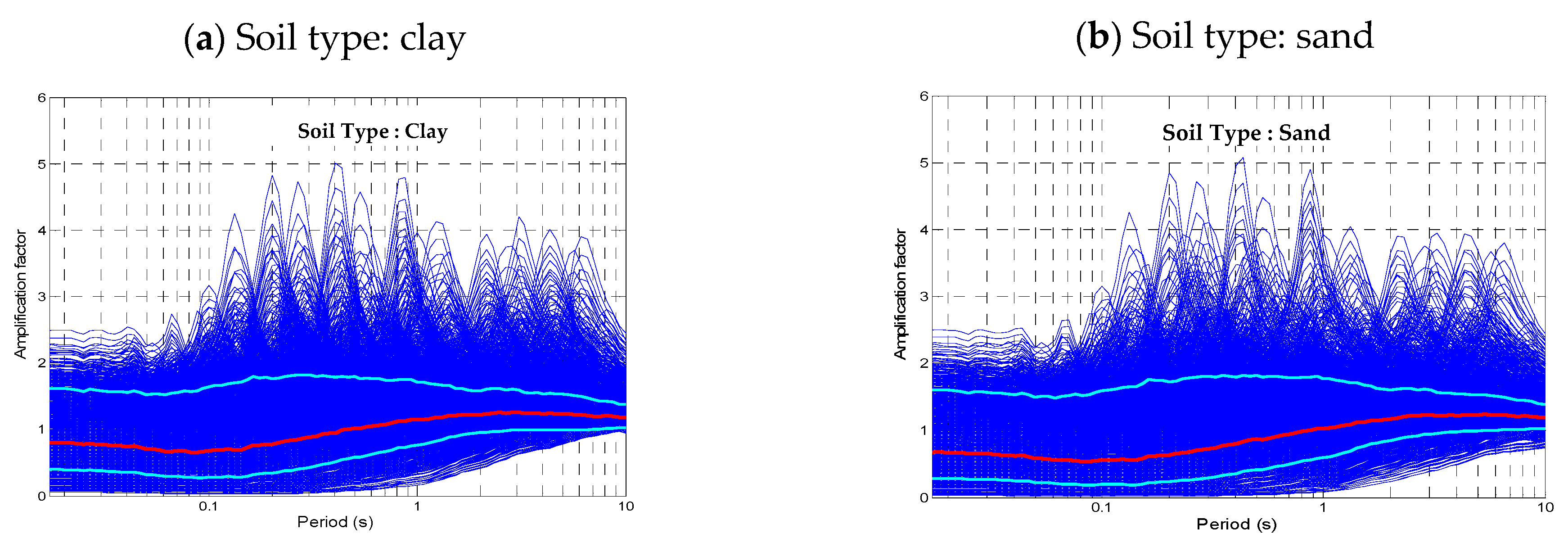
- For each profile set, we compute the , the average amplification factors (AFm), to constitute, for each soil type, a database of 3564 values and their associated variability , the mean amplification factor , and the associated initial variability . The results are displayed in Figure 6a,b for the clay and sand sets, respectively. The following main observations are derived:
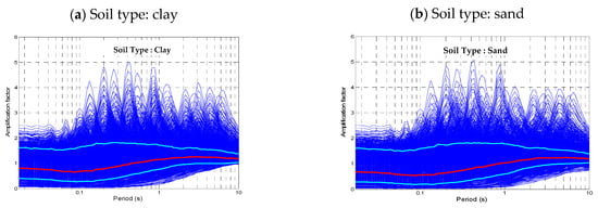 Figure 6. Average amplification factors as functions of real period for each set of soil profiles, namely (a) clay soil profiles and (b) sand soil profiles. Thin blue lines correspond to every site profile (3564 results), thick red line is geometrical average over whole profile sets, and thick light blue lines are averages ± one standard deviation.
 - The peak period, i.e., the period with the peak amplification factor, covers a very broad range from 0.08 s to about 6–7 s for clay and sand soil profiles, which explains the richness of the database.
- As shown in Figure 4 and Figure 5, the corresponding peak amplification ranges from less than 1.0 to 4.0 and up to 5.0 for low levels of PGA (0.01 g to 0.05 g). However, increasing the PGA level results in a decrease in the peak amplification factors to values of around 2.0 to 2.5 for a PGA ranging from 0.75 g to 1.05 g. The average amplification factors for clay are generally higher than those for sand at the mean (2 Hz ≤ f < 5 Hz) and high (f ≥ 5 Hz) frequency ranges.
- Some amplification factors exhibit a short period of de-amplification. A careful look at the corresponding soil profiles indicates that they correspond to deep soft soils, with low velocity, which act as seismic isolators.
- The overall average amplification factor (Figure 6a,b) is higher than unity for periods greater than 0.5 s for clay soil profiles, but it is greater than 0.9 s for sand soil profiles. The lowest overall average amplification factor is observed in the 0.05 to 0.15 s period range for clay and sand soil profiles. In this period range, the overall average amplification factor is less than 0.7 and 0.6 for clay and sand, respectively. The overall average amplification factors are significantly smaller than the peak values for individual profiles, which highlights the need to identify relevant site parameters that may explain this site-to-site variability.
- The “initial variability” associated with the average AFs (Table 3) has a maximum value at low to intermediate periods (0.01 to 0.4 s), reaching up to 0.39 for clay and 0.47 for sand soil. It then gradually vanishes with the period’s increase, reaching a value of around 0.065 at T = 10 s.
3.4. The Division of the Period Range: Short, Intermediate, and Long Periods
The UBC and the National Building Codes are based mainly on research works dating back to the 1990s [10,76]. These earlier studies recognized the dependency of the AF with the period and defined three representative amplification factors for three distinct zones: 1- Fa for the short period range (acceleration plateau); 2- Fv for the intermediate to long period range (velocity zone); and 3- Fl for the long period range. In this study, we adopt the same methodology and classification, and in the absence of any consensus regarding the limits of these zones, we use the following ranges: Fa is obtained by the mean AF value for periods in the [0.1 s, 0.2 s] range; Fv for periods in the [0.75 s, 1.5 s] range; and Fl, for periods in the [2.82 s, 5.65 s] range.
4. Description and Implementation of Neural Network Method
The principal objective of an artificial neural method is to predict or establish relationships between input and output parameters. It is particularly useful for developing simpler forms of relations between input and output parameters for cases where the interrelations between these parameters are complex and no obvious function exists to describe them. This method is essentially based on a training phase with a database, composed of input and output parameters, with the database being randomly selected. After the training phase is completed, the neuron network can basically be used to predict new input and associated output values for the parameters. In the field of seismology, this method has been used by many researchers to derive new GMPEs [35,36,37,38,39,77]. Two types of ANNs are used in this study: the Generalized Regression Neural Network (GRNN) and the Radial Basis Function (RBF), which are of the same family but with slightly different architecture. Both ANNs have three layers: an input layer, a hidden layer, and an output layer.
In this study, we used a GRNN for the identification of site proxies (input parameters) for both soil types, sand and clay. To this end, we used the 324 soil profiles (soil parameters) of each type for which 11 average amplification factors (i.e., were computed from the different seismic signal databases with different PGA values ranging from 0.01 g to 1.05 g. That is, there was a database of 3564 (324 × 11) cases for each soil type. The output consisted of the calculated AF values for the selected 100 periods of the structure and the amplification factors at short, intermediate, and long periods, named Fa, Fv, and Fl, respectively). Half of the database was used for training, and the second half for testing. Elements of these two subgroups of the database were selected and swapped randomly from one to the other until the network parameter, which is the Gaussian width for the GRNN, was determined. The main advantage of this method is the rapidity of the training phase. Note that many possible combinations of input site parameters were considered. The performance of the GRNN model was measured with various non-independent indicators, namely, the standard deviation of residuals, the reduction in variance with respect to the initial variability, the coefficient of correlation, and the physical tendency. Based on the results obtained with the GRNN, the combination of input site parameters giving the best performance while being handy for engineering practice were selected. For the selected combination of parameters, the RBF neural network was used to obtain a simple prediction equation. However, the training phase needs many adjustments, such as the number and the choice of key neurons in the hidden layer, and it is time-consuming. In the training phase of the RBF, the number and the choice of key neurons can either be set randomly from the training data, or they are iteratively trained or derived using techniques such as K-means, Max–Min algorithms, or Kohonen self-organizing maps [78,79,80,81,82,83,84,85,86,87,88,89,90,91,92,93]. After this unsupervised training was carried out and the number and key neurons in the hidden layer were chosen, the weights between this layer and the output layer neurons were determined by multiple regressions in a supervised manner. We used cross-validation, with 50% of the data used for training and the remaining 50% for testing, with each half of the database randomly being swapped from one to other until the RBF network parameters were obtained. More details about the used neural networks and their implementation are given in the Supplementary File, section (d).
5. Results
This section summarizes the main findings and results from the above process, combining a GRNN and RBF.
5.1. Determination of Site Proxies Using GRNN
A total of 200 GRNN models using different combinations of input parameters were derived, and their results were analyzed and compared in terms of the standard deviation of residuals (predicted–actual values) to the initial standard deviation values for each period, i.e., and the overall variability defined earlier.
Equations (22) and (23) are used to compute the error between predicted and actual values, which in turn are compared with the initial variabilities found using Equations (18)–(21).
The standard deviation of residuals for each period and each neural network model, for comparison with the initial variability term is given by the following:
where the ANN is GRNN or RBF.
The maximum standard deviation over all periods is defined as
The overall error is defined as the average over all periods of the error term, that is,
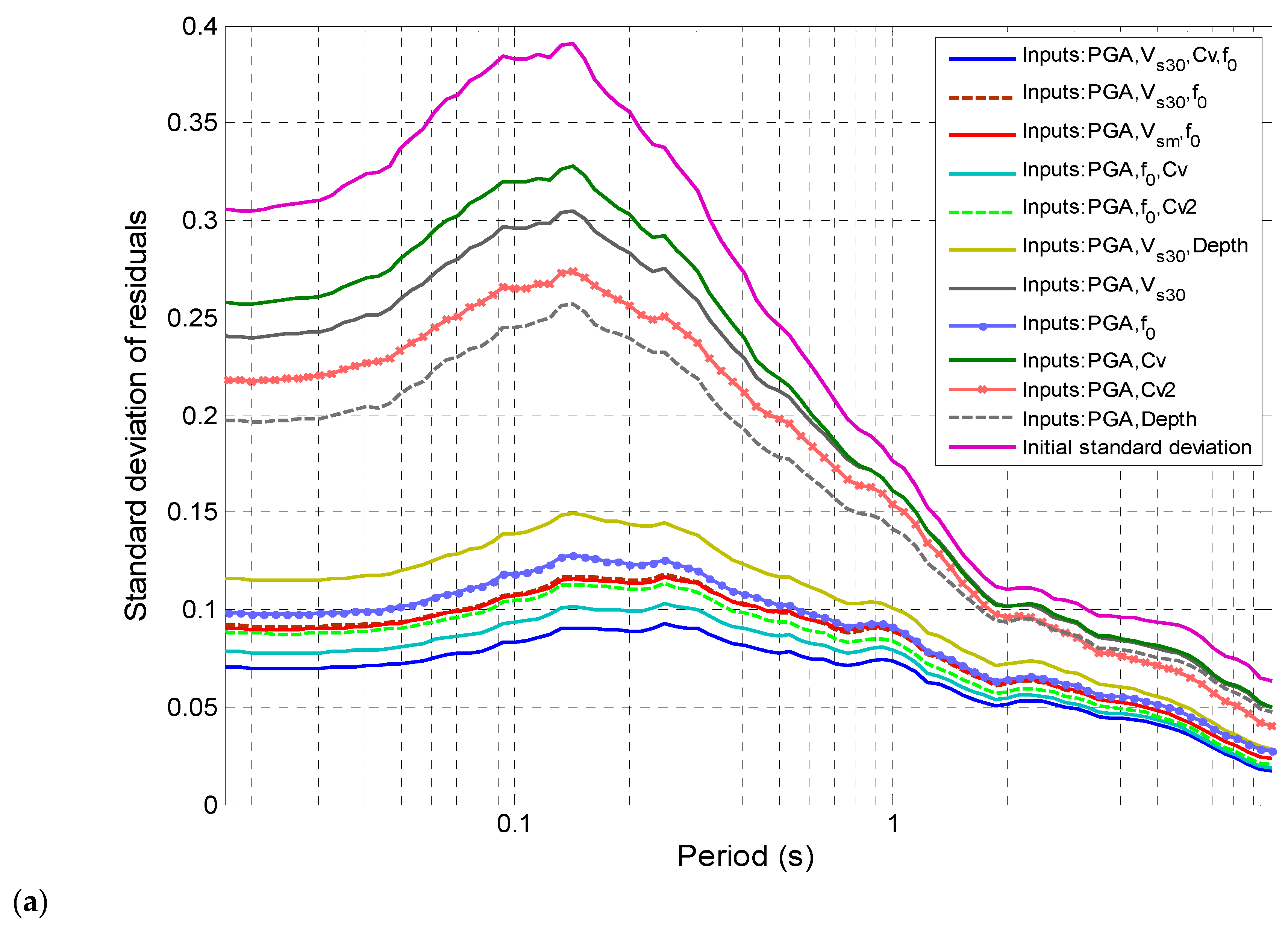
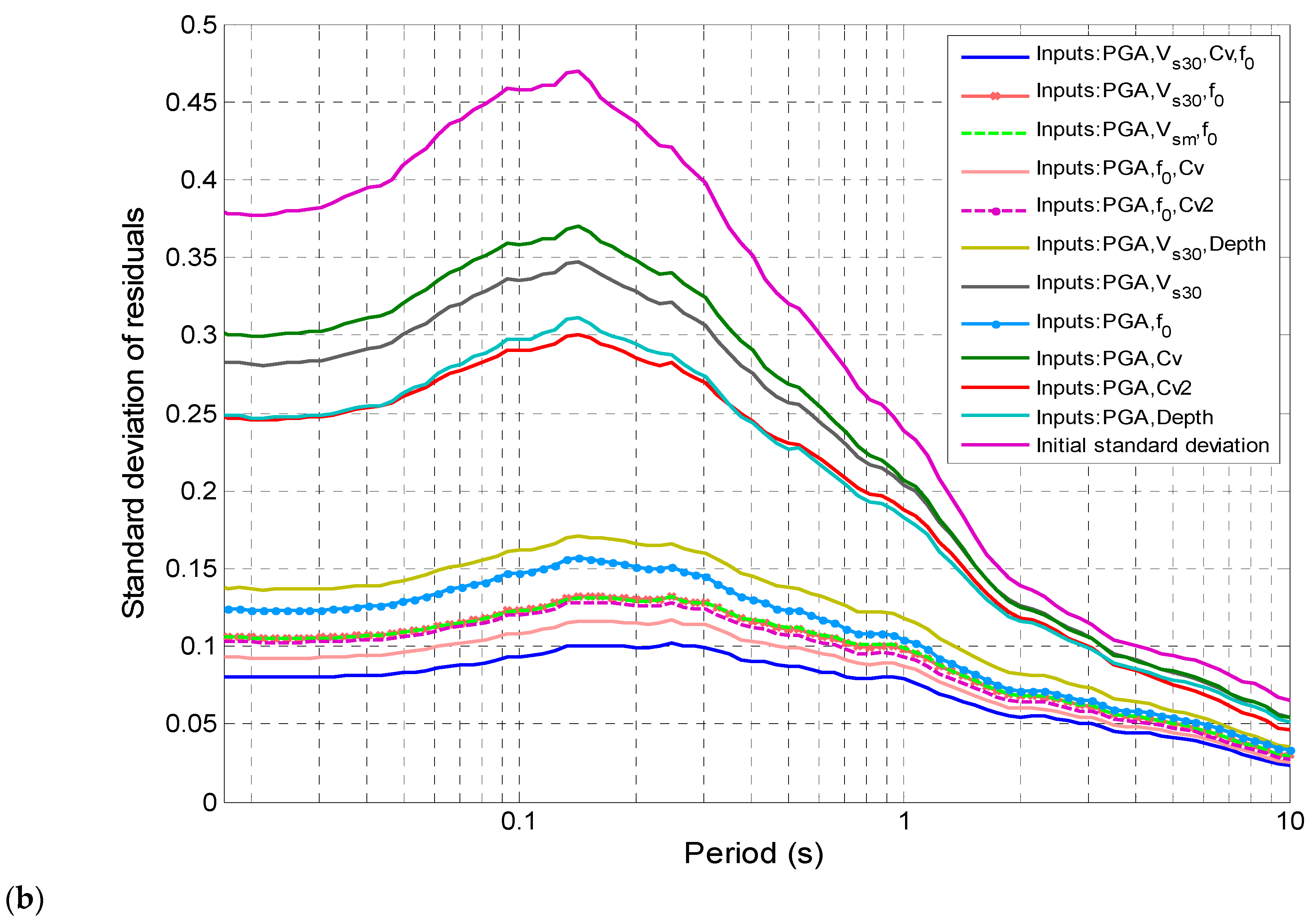
To obtain a statistically meaningful insight into the relative performances of each site proxy considered in controlling the amplification factor, the standard deviation for each soil type and period error term is plotted, together with the initial variability, , in Figure 7a,b for clay and sand soil profiles, respectively.
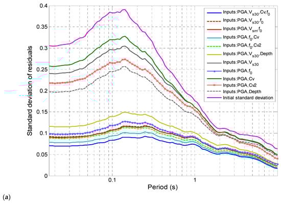
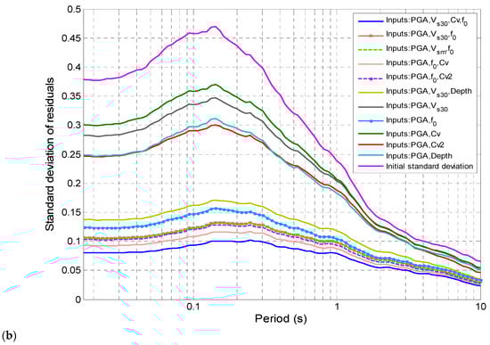
Figure 7.
Variations in root mean square error and standard deviation of residuals for various GRNN models with various sets of input site parameters compared to initial variability (a) for clay soil profiles and (b) for sand soil profiles. Data are displayed as function of real period.
In order to better identify the importance of the site proxy, the reduction in the overall standard deviation of residuals is defined by:
Table 4 presents the overall standard deviation of residuals as well as the reduction in the standard deviation of residuals for different GRNN models using different input parameter combinations.
Table 4.
Standard deviations of model residuals and reduction in standard deviation for various GRNN models involving initial actual frequency amplification factors (clay and sand soil profiles) for various site parameter combinations.
Figure 7a,b exhibit several noticeable features:
- The PGA is common to all input parameter combinations. The model did not converge when not considering the PGA nor when considering only a single parameter. This means that the PGA is a predominant input parameter, and at the very least, a couple of PGAs with another parameter are needed to achieve convergence.
- The PGA and f0 constitute the best couple for the prediction of the amplification factor, producing 64% to 65% reductions in the standard deviation for clay and sand soil profiles, respectively. The PGA performs well for all periods and soil types. In comparison, all other couples of parameters offer a lower reduction in variability, capped at 33%.
- The triplet (PGA, Cv, f0) is the most pertinent triplet for predicting the AF, with a standard deviation reduction of more than 71% for clay and 73% for sand profiles. The other triplets (PGA, Cv2, f0), (PGA, Vsm, f0), and (PGA, Vs30, f0), which present interesting but slightly lower performances, are also worthy of consideration. However, because parameters such as Cv and Cv2 are difficult to measure in practice and have less physical meaning, the triplet (PGA, Vs30, f0) is the triplet retained for predicting the AF. Considering more than three parameters will lead to better predictions, but for practical reasons, we decided not to go further.
- The largest root mean square errors are systematically found in short to intermediate period ranges (see Figure 7).
5.2. Variation in Amplification Factors for Specific Period Ranges Using RBF
Design codes take into account site effects via multiplying the design spectra by amplification factors (i.e., F(T) in the CNBC). These amplification factors vary with the period of the structure and soil properties. For the sake of simplicity and with respect to earlier versions of codes (i.e., CNB2005), we consider averaged site factors for three specific ranges: Fa for short periods; Fv for intermediate periods; and Fl for long periods.
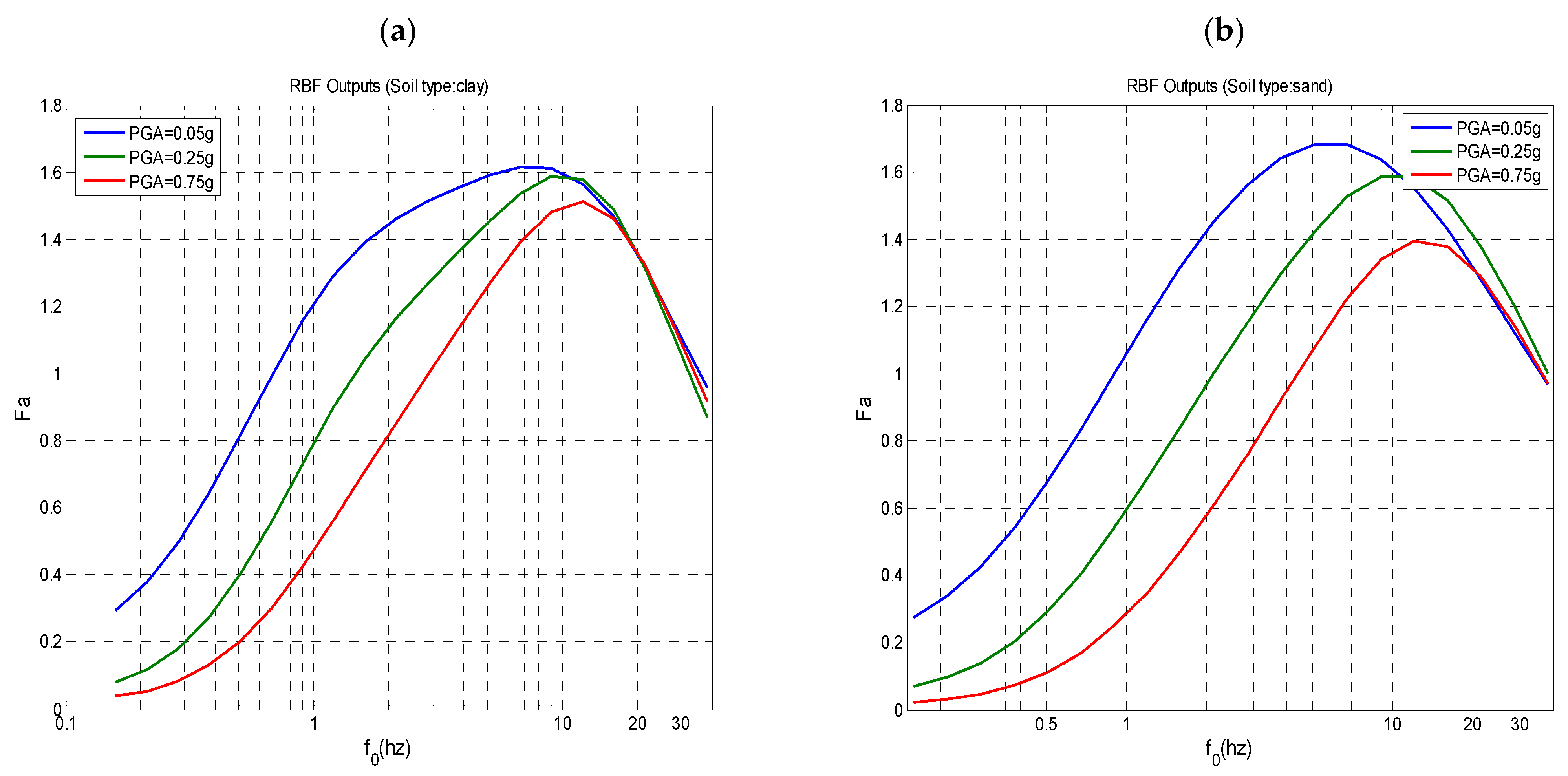
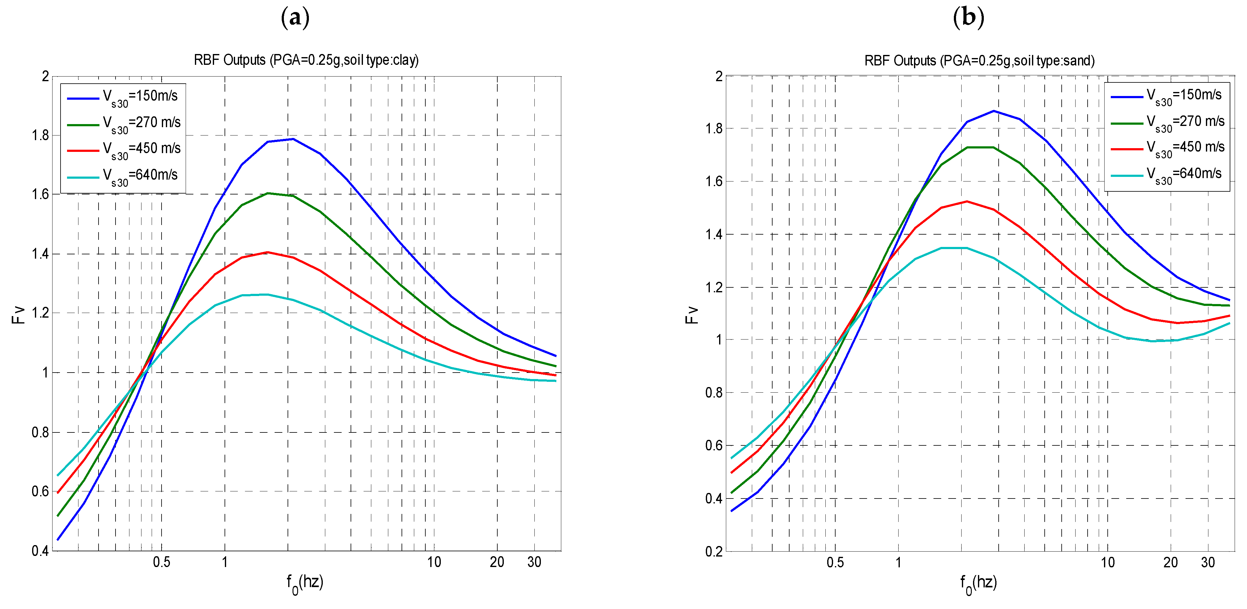
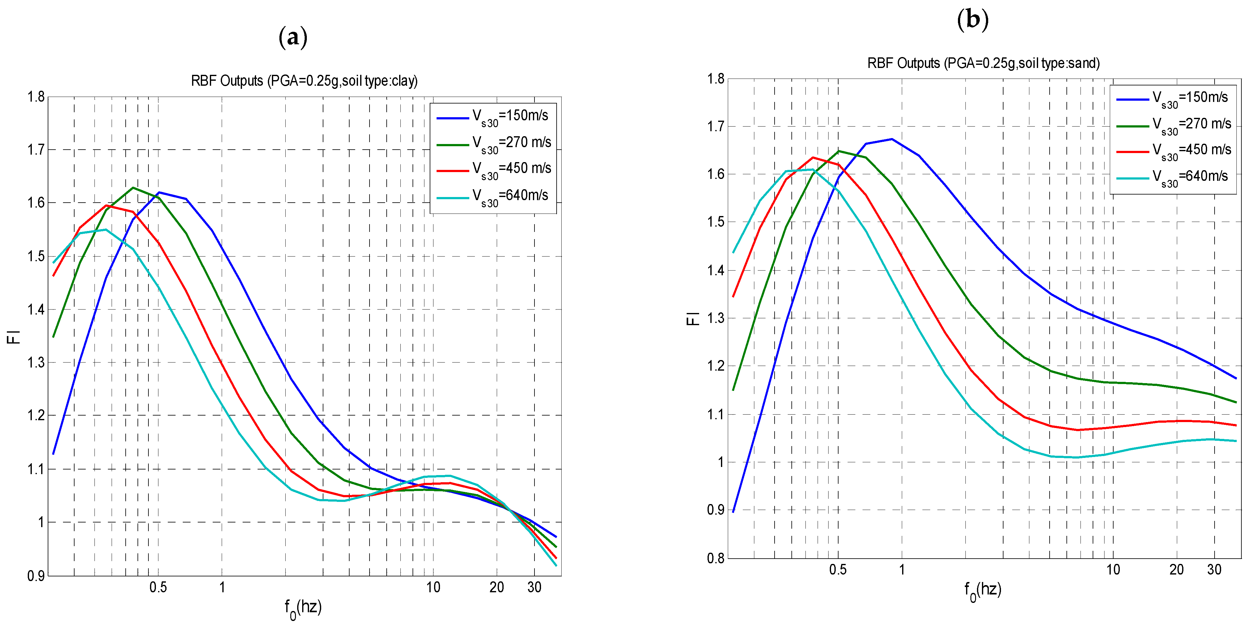
In this section, we compute these amplification factors, Fa, Fv, and Fl, from the RBF model based on the triplet , which proved to be efficient and accurate. Figure 8, Figure 9, Figure 10 and Figure 11 display the dependence of these three factors, PGA, . The [0.15, 40 Hz] interval is considered for in all cases, covering the full range of the database. In Figure 8, the results are computed for a value varying within the frequency range studied, while in the other figures, typical low (150 m/s), mid (270 m/s), high (450 m/s), and very high (640 m/s) values of are considered. The intensity of the seismic excitation is displayed for three (03) discrete levels: PGA = 0.05 g, 0.25 g, and 0.75 g.
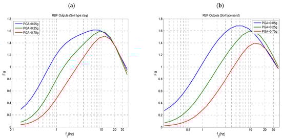
Figure 8.
Variations in the short period amplification factors, Fa, with f0 for different PGA values: 0.05 g, 0.25 g, and 0.75 g. (a) Clay soil profiles; (b) sand soil profiles.
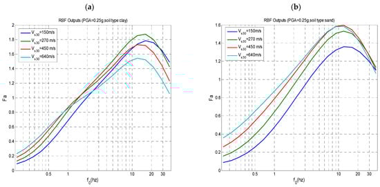
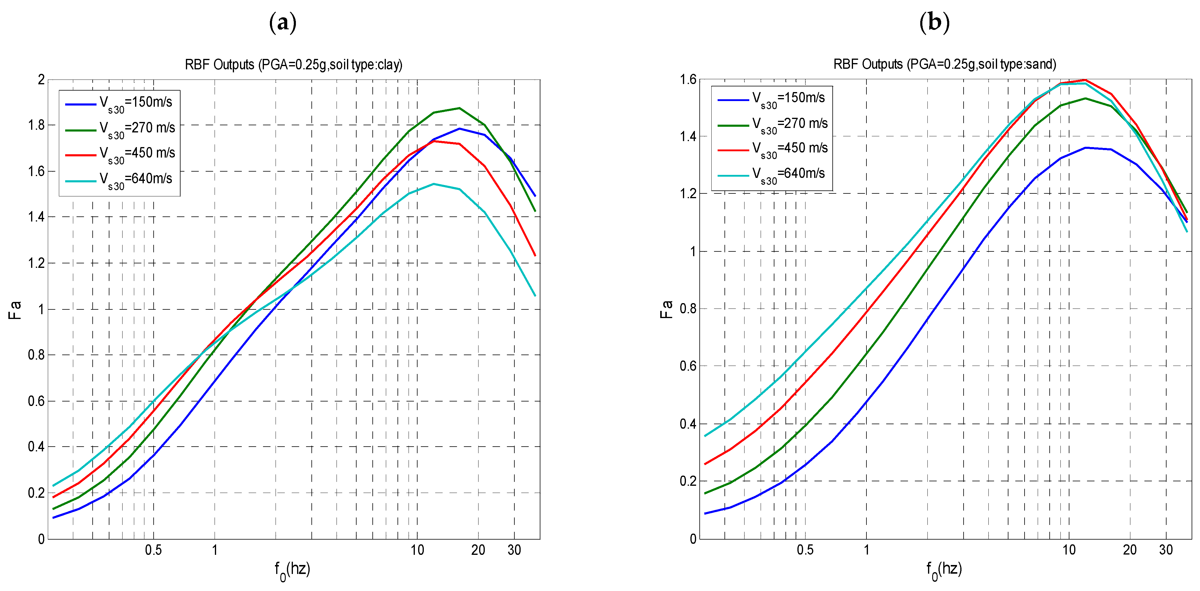
Figure 9.
Variation in amplification factor at short period Fa with f0 and PGA for four values of Vs30 (150, 270, 450, and 640 m/s) (a) for clay soil profiles and (b) for sand soil profiles.
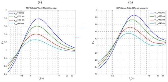
Figure 10.
Variation in amplification factor at mid period Fv with f0 and PGA for four values of Vs30 (150, 270, 450, and 640 m/s) (a) for clay soil profiles and (b) for sand soil profiles.
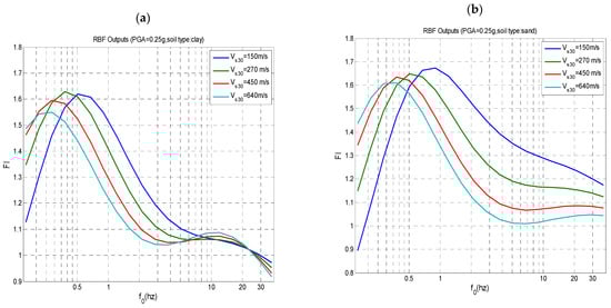
Figure 11.
Variation in amplification factor at long period Fl with f0 and PGA for four values of Vs30 (150, 270, 450, and 640 m/s) and PGA (a) for clay soil profiles and (b) for sand soil profiles.
Table 5 presents a summary of the statistical parameters obtained by the RBF triplet predictions. As shown, the initial standard deviation of the residuals is greatly reduced by a factor ranging roughly from 3 to 30. Excellent coefficients of determination, R2, are obtained and are greater than 0.91, ranging from 0.96 to 0.99 for Fa and Fv for both soil types.
Table 5.
Standard deviation of model residuals, coefficient of determination R2, and numbers of key neurons in hidden layer determined after training phase for various RBF models at short, mid, and long periods (Fa, Fv, and Fl) for clay and sand soil profiles for combination of three soil parameters (PGA, f0, and Vs30).
The values of Fa, Fv, and Fl may be predicted as a function of , , and PGA using the following explicit equation based on RBF models:
where a1 is a vector of t lines output by the hidden layer, with t being the number of key neurons in the hidden layer, determined from the training phase. It is estimated from their Euclidian distance (see Section 3 of Supplementary File) using the following equation:
where we1, we2, and we3 can be expressed by
we1, we2, and we3 are vectors of t lines, while b1 and b2 are the biases determined after the training phase.
To investigate the performance of the RBF model, we consider only 50% of the data for training and the other for testing. The main results obtained are summarized in Table 6 in terms of the standard deviation and coefficient of determination (R2). They demonstrate the good performance of the model.
Table 6.
Performance of RBF model on interpolation, results on terms. Standard deviation of model residuals and coefficient of determination R2 for database test at Fa, Fv. and Fl for clay and sand.
The following regression equation between Vs30 and f0 is derived from the obtained predictions of the RBF model:
From the results of Figure 8, Figure 9, Figure 10 and Figure 11 (and similar results for Fv and Fl), we note the following findings:
- Generally, the amplification factors Fa, Fv, and Fl, are higher for clay-type soil than for sand-type soil. This is particularly true for the range of low frequencies f0 up to 1 Hz. However, for f0 values higher than 3 Hz and for relatively stiff soils, with a value exceeding 350 m/s, Fa and Fv values are slightly higher for sand than for clay.
- The amplification factors are higher for low PGA values. This holds true for the factor Fl and soft soils with low values.
Furthermore, from the results of Figure 9, we can note that the correlations between f0 and Vs30 given by Equation (31) are not always respected as the frequency f0 does not increase systematically with the Vs30 value at the peak value of the amplification factors. This is explained by the following two factors:
- -
- Some combinations are not possible in real cases, such as having a soil profile with a fundamental frequency f0 greater than 10 Hz while its Vs30 value is lower than 500 m/s. In such situations, the predictions of Equation (26) are somehow extrapolations that are very likely erroneous and meaningless.
- -
- The predictions of Equation (26) shall be considered for explaining the global tendency regarding the interactions between different parameters such as the change in the amplification factors with the PGA level, Vs30 (about 600 m/s). We can observe, for instance, that stiff soils with high Vs30 values have higher Fa but lower Fl than soft soils with low values of Vs30 (about 150 m/s). Similarly, the tendencies of Fv and Fl with Vs30 and PGA can be deduced from the results shown in Figure 10 and Figure 11, respectively.
Based on the RBF neural network, we can compute the synaptic weight, which characterizes the respective impacts of each of the three input parameters considered, namely, PGA, Vs30, and f0 (see Supplementary File, section (e)). The resulting synaptic weights and the main results of these computed weights are reported in Table 7. We observe that generally, the fundamental frequency f0 has the highest synaptic weight, which is typically more than 45% for clay soil profiles, and there are even higher values of the synaptic weight for Fa and Fv values of sand soil profiles. The PGA synaptic weight is generally of secondary importance, except in the case of the amplification factor Fl in a sand soil profile, where it is the highest.
Table 7.
Participation of synaptic weights for different site parameters used in RBF model.
6. Conclusions
The main objective of this study was to identify the key soil parameters influencing 1D site seismic response and amplification factors (AFs) at the free surface. To achieve this, we computed the nonlinear site response using a linear equivalent approach under vertically incident plane waves, utilizing a representative set of real input accelerograms that cover a broad range of peak frequencies and intensities.
We focused on monolayer soil profiles with variable thicknesses and shear wave velocities, situated above a semi-infinite bedrock with varying shear wave velocities. Soil nonlinearity was modelled using degradation curves proposed by Sun et al. (1988) [58] for clay and Seed and Idriss (1970) [52] for sand, which are simple and require minimal soil parameters and are effective enough. In total, 324 soil profiles of sand and an equal number of profiles of clay were analyzed under 14 records at 11 PGA levels each for a total of 99,792 time-history analyses.
For each soil profile, we calculated geometric average amplification factors for short to mid and long period ranges, denoted as Fa, Fv, and Fl for periods of [0.1 s, 0.2 s], [0.75 s, 1.5 s], and [2.82 s, 5.65 s], respectively.
Two types of neural networks were utilized in our analysis: (1) the Generalized Regression Neural Network (GRNN) was used to identify the most effective combination of soil proxies in predicting AFs, and (2) the Radial Basis Function neural network (RBF) was used to develop regression equations between these proxies and AFs. This combination of methods facilitated a comprehensive investigation into the factors that govern site response. The main findings can be summarized as follows:
- The pair (PGA, f0) was identified as effective for predicting AFs, achieving reductions in the standard deviation of 64% and 65% for clay and sand profiles, respectively.
- The triplet (PGA, Cv, f0) proved to be particularly powerful in predicting actual AFs, resulting in standard deviation reductions of over 71% for both clay and sand. Other combinations, such as (PGA, Cv2, f0), (PGA, Vsm, f0), and (PGA, Vs30, f0), also yielded promising results and can be utilized.
- Because parameters Cv and Cv2 are often difficult and costly to measure in engineering practices, we recommend using the combination (PGA, Vs30, f0), which, while offering slightly lower performance, still provides a significant reduction in the standard deviation, making it a practical alternative for field applications.
Furthermore, the prediction equations derived from the GRNN were found to be quite complex due to the high number of neurons in the hidden layer, making them challenging to implement in practice. As a result, we opted for the RBF neural network, which offers simpler prediction equations, albeit at the cost of a more intensive and prolonged training phase. We focused on the most effective site proxies identified through the GRNN analysis: PGA, f0, and Vs30. Using the RBF, we established correlation relationships between these proxies and site-specific average AFs, considering the variability in initial AFs across the 3564 values for each soil type. Both the overall period range and specific short- and mid- to long-period ranges associated with the amplification factors Fa, Fv, and Fl were analyzed.
Using 50% of the database for training and the remaining 50% for testing, the RBF results demonstrated a lower standard deviation of the error term (εRBF) for Fa, Fv, and Fl, generally with a reduction in the standard deviation exceeding 61%, along with a strong coefficient of determination exceeding 91%. These findings highlight the effectiveness of the RBF neural network method in accurately predicting amplification factors.
The main findings of this study will aid in enhancing site classification by establishing a physical relationship between the AF and site proxies. However, several recommendations regarding regulatory codes can be made:
- The Inclusion of the Fundamental Frequency: The fundamental frequency (f0) should be considered alongside the peak ground acceleration (PGA) and shear wave velocity (Vs30) to improve predictions of amplification factors.
- The Distinction of Period Ranges: It is crucial to differentiate between amplification factors for short (Fa), medium (Fv), and long (Fl) period ranges. The long-period amplification (Fl) is particularly significant, often exceeding Fa and Fv values for soil profiles with low Vs30 values, which typically correspond to site classes C, D, and E in Eurocode 8 (EC8) and site classes D and E in UBC/CNBC codes.
Finally, we propose new equations for predicting the amplification factor across specific short-, mid-, and long-period ranges.
It is important to acknowledge the limitations of this study, primarily related to the use of simplistic soil profiles (homogeneous, monolayer, and 1D) and basic degradation curves, specifically those used by Sun et al. (1988) [58] for clay and Seed and Idriss (1970) [52] for sand. Adopting more recent degradation curves and realistic soil profiles and site geometry could yield more accurate and site-specific amplification factors. Nevertheless, this study provides straightforward and effective prediction equations for amplification factors, utilizing a limited number of parameters that could enhance current design codes.
Supplementary Materials
The following supporting information can be downloaded at: https://www.mdpi.com/article/10.3390/app15073618/s1.
Author Contributions
Conceptualization, A.B.S.; Methodology, A.B.S.; Validation, L.G.; Investigation, A.B.S.; Writing—original draft, A.B.S.; Writing—review & editing, L.G.; Funding acquisition, L.G. All authors have read and agreed to the published version of the manuscript.
Funding
This work was partially supported by the Ecole de technologie superieure, University of Québec, 1100 Notre-Dame Ouest, Montréal, QC H3C 1K3, Canada: https://www.etsmtl.ca/ and by the Fonds de recherche du Quebec: https://frq.gouv.qc.ca/.
Institutional Review Board Statement
Not applicable.
Informed Consent Statement
Not applicable.
Data Availability Statement
The original contributions presented in this study are included in the article/Supplementary Material. Further inquiries can be directed to the corresponding author.
Acknowledgments
The department of Construction Engineering of Ecole de technologie superieure and its staff for their support and material resources used along the project.
Conflicts of Interest
The authors declare no conflicts of interest.
References
- Bard, P.-Y.; Campillo, M.; Chavez-Garcia, F.J.; Sanchez-Sesma, F.J. The Mexico Earthquake of September 19, 1985—A Theoretical Investigation of Large- and Small-scale Amplification Effects in the Mexico City Valley. Earthq. Spectra 1988, 4, 609–633. [Google Scholar] [CrossRef]
- Kawase, H.; Aki, K. A study on the response of a soft soil basin for incident S, P, and Rayleigh waves with special reference to the long duration observed in Mexico City. Bull. Seismol. Soc. Am. 1989, 79, 1361–1382. [Google Scholar]
- Chávez-García, F.J.; Bard, P.Y. Site effects in Mexico City eight years after the September 1985 Michoacan earthquakes. Soil Dyn. Earthq. Eng. 1994, 13, 229–247. [Google Scholar]
- Del Gaudio, V.; Pierri, P.; Rajabi, A.M. An approach to identify site response directivity of accelerometer sites and application to the Iranian Area. Pure Appl. Geophys. 2015, 172, 1471–1490. [Google Scholar] [CrossRef]
- Cherid, D.; Hammoutene, M.; Tiliouine, B.; Berrah, M.K. Local seismic site amplification: Effects of obliquely incident antiplane motions. J. Seismol. 2017, 21, 509–524. [Google Scholar] [CrossRef]
- Sandıkkaya, M.A.; Akkar, S. Cumulative absolute velocity, Arias intensity and significant duration predictive model from a pan-European strong-motion dataset. Bull. Earthq. Eng. 2017, 15, 1881–1898. [Google Scholar] [CrossRef]
- Boudghene Stambouli, A.; Zendagui, D.; Bard, P.Y.; Dif, H. Influence of site parameters on fourier amplification application for 1D linear viscoelastic method. Period. Polytech. Civ. Eng. 2021, 65, 229–241. [Google Scholar] [CrossRef]
- Dif, H.; Boudghene Stambouli, A. Impact of site condition on Arias intensity and Cumulative absolute velocity: Application for low seismicity areas. Asian J. Civ. Eng. 2023, 24, 1411–1424. [Google Scholar] [CrossRef]
- Buckle, I.G.; Friedland, I.; Mander, J.; Martin, G.; Nutt, R.; Power, M. Seismic Retrofitting Manual for Highway Structures. Part 1, Bridges (No. FHWA-HRT-06-032); Turner-Fairbank Highway Research Center: McLean, VA, USA, 2006.
- Borcherdt, R.D. Estimates of site dependent response spectra for design (methodology and justification). Earthq. Spectra 1994, 10, 617–653. [Google Scholar] [CrossRef]
- Martin, G.R.; Dobry, R. Earthquake site response and seismic code provisions. NCEER Bull. 1994, 8, 1–6. [Google Scholar]
- Dickenson, S.E.; Seed, R.B. Nonlinear Dynamic Response of Soft and Deep Cohesive Soil Deposits. In Proceedings of the International Workshop on Site Response Subjected to Strong Earthquake Motions, Yokosuka, Japan, 16–17 January 1996; Volume 2, pp. 67–81. [Google Scholar]
- Dobry, R.; Borcherdt, R.D.; Crouse, C.B.; Idriss, I.M.; Joyner, W.N.; Martin, G.R.; Power, M.S.; Rinne, E.E.; Seed, R.B. New Site coefficients and site classification system used in recent building seismic code provisions. Earthq. Spectra 2000, 16, 41–67. [Google Scholar] [CrossRef]
- Steidl, J.H. Site response in southern California for probabilistic seismic hazard analysis. Bull. Seismol. Soc. Am. 2000, 90, S149–S169. [Google Scholar] [CrossRef]
- Rodriguez-Marek, A.; Bray, J.D.; Abrahamson, N.A. An empirical geotechnical seismic site response procedure. Earthq. Spectra 2001, 17, 65–87. [Google Scholar] [CrossRef]
- Pitilakis, K.D.; Makra, K.A.; Raptakis, D.G. 2D vs 3D Site Effects with Potential Applications to Seismic Norms: The case of EUROSEISTEST and Thessaloniki. In Proceedings of the XVth ICSMGE, Istanbul, Turkey, 27–31 August 2001; pp. 123–133. [Google Scholar]
- Stewart, J.P.; Liu, A.H.; Choi, Y. Amplification Factors for Spectral Acceleration in Tectonically Active Regions. Bull. Seismol. Soc. Am. 2003, 93, 332–352. [Google Scholar] [CrossRef]
- Choi, Y.; Stewart, J.P. Nonlinear site amplification as function of 30 m shear wave velocity. Earthq. Spectra 2005, 21, 1–30. [Google Scholar] [CrossRef]
- Castellaro, S.; Mulargia, F.; Rossi, P.M. Vs30: Proxy for seismic amplification? Seismol. Res. Lett. 2008, 79, 540–543. [Google Scholar] [CrossRef]
- Lee, V.W.; Trifunac, M.D. Should average shear-wave velocity in the top 30m of soil be used to describe seismic amplification? Soil Dyn. Earthq. Eng. 2010, 30, 1250–1258. [Google Scholar] [CrossRef]
- Abrahamson, N.; Atkinson, G.; Boore, D.; Bozorgnia, Y.; Campbell, K.; Chiou, B.; Idriss, I.; Silva, W.; Youngs, R. Comparisons of the NGA ground-motion relations. Earthq. Spectra 2008, 24, 45–66. [Google Scholar] [CrossRef]
- Gregor, N.; Abrahamson, N.A.; Atkinson, G.M.; Boore, D.M.; Bozorgnia, Y.; Campbell, K.W.; Chiou, B.S.-J.; Idriss, I.M.; Kamai, R.; Seyhan, E.; et al. Comparison of NGA-West2 GMPEs. Earthq. Spectra 2014, 30, 1179–1197. [Google Scholar] [CrossRef]
- Ancheta, T.D.; Darragh, R.B.; Stewart, J.P.; Seyhan, E.; Silva, W.J.; Chiou, B.S.-J.; Wooddell, K.E.; Graves, R.W.; Kottke, A.R.; Boore, D.M.; et al. NGA-West 2 database. Earthq. Spectra 2014, 30, 989–1005. [Google Scholar] [CrossRef]
- Douglas, J.; Akkar, S.; Ameri, G.; Bard, P.-Y.; Bindi, D.; Bommer, J.J.; Singh Bora, S.; Cotton, F.; Derras, B.; Hermkes, M.; et al. Comparisons among the five ground-motion models developed using RESORCE for the prediction of response spectral accelerations due to earthquakes in Europe and the Middle East. Bull. Earthq. Eng. 2014, 12, 341–358. [Google Scholar] [CrossRef]
- Luzi, L.; Puglia, R.; Pacor, F.; Gallipoli, M.; Bindi, D.; Mucciarelli, M. Proposal for a soil classification based on parameters alternative or complementary to Vs, 30. Bull. Earthq. Eng. 2011, 9, 1877–1898. [Google Scholar] [CrossRef]
- Cadet, H.; Bard, P.-Y.; Duval, A.-M.; Bertrand, E. Site effect assessment using KiK-net data—Part 2—Site amplification prediction equation (SAPE) based on f0 and Vsz. Bull. Earthq. Eng. 2012, 10, 451–489. [Google Scholar] [CrossRef]
- Pitilakis, K.; Riga, E.; Anastasiadis, A. Design spectra and amplification factors for Eurocode 8. Bull. Earthq. Eng. 2012, 10, 1377–1400. [Google Scholar] [CrossRef]
- Pitilakis, K.; Riga, E.; Anastasiadis, A. New code site classification, amplification factors and normalized response spectra based on a worldwide ground-motion database. Bull. Earthq. Eng. 2013, 11, 925–966. [Google Scholar] [CrossRef]
- NEHRP Guidelines for the Seismic Rehabilitation of Buildings; FEMA-273; Federal Emergency Management Agency: Washington, DC, USA, 1997. Available online: https://courses.washington.edu/cee518/fema273.pdf (accessed on 10 March 2025).
- Uniform Building Code. Structural engineering design provisions. In Proceedings of the International Conference of Building Officials, Whittier, CA, USA, 14 July 1997; Volume 2. [Google Scholar]
- EN 1998-1; EC8 Eurocode 8. Design of Structures for Earthquake Resistance—Part 1: General Rules, Seismic Actions and Rules for Buildings. European Committee for Standardization (CEN): Brussels, Belgium, 2004. Available online: https://eurocodes.jrc.ec.europa.eu (accessed on 1 February 2016).
- IBC2012. International Building Code, 2012 ed.; International Code Council: Washington, DC, USA, 2012; ISBN 978-1-60983-039-7. Available online: https://archive.org/details/gov.law.icc.ibc.2012 (accessed on 1 November 2016).
- Canadian Commission on Building and Fire Codes, National Research Council of Canada. National Building Code of Canada (NBC) (2015) National Building Code of Canada; Canadian Commission on Building and Fire Codes, National Research Council of Canada: Ottawa, ON, Canada, 2015. [Google Scholar]
- Canadian Commission on Building and Fire Codes, National Research Council of Canada. National Building Code of Canada (NBC) (2015b) User’s Guide—NBC 2015 Structural Commentaries (Part 4 of Division B); Canadian Commission on Building and Fire Codes, National Research Council of Canada: Ottawa, ON, Canada, 2015. [Google Scholar]
- Boudghene Stambouli, A.; Zendagui, D.; Bard, P.-Y.; Derras, B. Deriving amplification factors from simple site parameters using generalized regression neural networks: Implications for relevant site proxies. Earth Planets Space 2017, 69, 99. [Google Scholar] [CrossRef]
- Ghaboussi, J.; Garrett, J., Jr.; Wu, X. Knowledge-based modeling of material behavior with neural networks. J. Eng. Mech. 1991, 117, 132–153. [Google Scholar] [CrossRef]
- Ghaboussi, J.; Sidarta, D. New nested adaptive neural networks (NANN) for constitutive modeling. Comput. Geotech. 1998, 22, 29–52. [Google Scholar] [CrossRef]
- Paolucci, R.; Colli, P.; Giacinto, G. Assessment of seismic site effect in 2-D alluvial Valleys Using Neural Networks. Earthq. Spectra 2000, 16, 661–680. [Google Scholar] [CrossRef]
- Hurtado, J.; Londono, J.; Meza, M. On the applicability of neural networks for soil dynamic amplification analysis. Soil Dyn. Earthq. Eng. 2001, 21, 579–591. [Google Scholar] [CrossRef]
- Derras, B.; Bard, P.Y.; Cotton, F.; Bekkouche, A. Adapting the neural network approach to PGA prediction: An example based on the KiK-net data. Bull. Seismol. Soc. Am. 2012, 102, 1446–1461. [Google Scholar] [CrossRef]
- Poggio, T.; Girosi, F. Networks for approximation and learning. Proc. IEEE 1990, 78, 1481–1497. [Google Scholar] [CrossRef]
- Liu, S.; Wang, L.; Zhang, W.; Sun, W.; Wang, Y.; Liu, J. Physics-informed optimization for a data-driven approach in landslide susceptibility evaluation. J. Rock Mech. Geotech. Eng. 2024, 16, 3192–3205. [Google Scholar] [CrossRef]
- Zhang, Z.; Pan, Q.; Yang, Z.; Yang, X. Physics-informed deep learning method for predicting tunnelling-induced ground deformations. Acta Geotechnica 2023, 18, 4957–4972. [Google Scholar] [CrossRef]
- Constantopoulos, I.V.; Roesset, J.M.; Christian, J.T. A comparison of linear and exact nonlinear analysis of soil amplification. In Proceedings of the 5th WCEE, Rome, Italy, 25–29 June 1973; pp. 1806–1815. [Google Scholar]
- Yoshida, N.; Kobayashi, S.; Suetomi, I.; Miura, K. Equivalent linear method considering frequency dependent characteristics of stiffness and damping. Soil Dyn. Earthq. Eng. 2002, 22, 205–222. [Google Scholar] [CrossRef]
- Assimaki, D.; Kausel, E. An equivalent linear algorithm with frequency-and pressure-dependent moduli and damping for the seismic analysis of deep sites. Soil Dyn. Earthq. Eng. 2002, 22, 959–965. [Google Scholar] [CrossRef]
- Johari, A.; Momeni, M. Stochastic analysis of ground response using non-recursive algorithm. Soil Dyn. Earthq. Eng. 2015, 69, 57–82. [Google Scholar] [CrossRef]
- Trifunac, M.D.; Todorovska, M.I. Can aftershock studies predict site amplification factors? Northridge, CA, earthquake of 17 January 1994. Soil Dyn. Earthq. Eng. 2000, 19, 233–251. [Google Scholar] [CrossRef]
- Nguyen, X.D.; Guizani, L. On the application limits and performance of the single-mode spectral analysis for seismic analysis of isolated bridges in Canada. Can. J. Civ. Eng. 2022, 49, 1747–1763. [Google Scholar] [CrossRef]
- Boudghene Stambouli, A.; Bard, P.Y.; Chaljub, E.; Moczo, P.; Kristek, J.; Stripajova, S.; Durand, C.; Zendagui, D.; Derras, B. 2D/1D aggravation factors: From a comprehensive study to estimation with a neural network model. In Proceedings of the 16Ith European Conference of Earthquake Engineering, Thessaloniki, Greece, 18–21 June 2018. [Google Scholar]
- Paolucci, R.; Morstabilini, L. Non-dimensional site amplification functions for basin edge effects on seismic ground motion. In Proceedings of the Third International Symposium on the Effects of Surface Geology on Seismic Motion, Grenoble, France, 30 August–1 September 2006; Volume 30, pp. 823–831. [Google Scholar]
- Seed, H.B.; Idriss, I.M. Soil Moduli and Damping Factors for Dynamic Response Analyses; EERC-70-10; University of California Berkeley Structural Engineers and Mechanics: Berkeley, CA, USA, 1970. [Google Scholar]
- Vucetic, M.; Dobry, R. Cyclic triaxial strain-controlled testing of liquefiable sands. In Advanced Triaxial Testing of Soil and Rock, ASTM STP 977; ASTM International: West Conshohocken, PA, USA, 1988. [Google Scholar]
- Vucetic, M.; Dobry, R. Effect of soil plasticity on cyclic response. J. Geotech. Eng. 1991, 117, 89–107. [Google Scholar] [CrossRef]
- Ishibashi, I.; Zhang, X. Unified dynamic shear moduli and damping ratios of sand and clay. Soils Found. 1993, 33, 182–191. [Google Scholar] [CrossRef]
- EPRI. Guidelines for Determining Design Basis Ground Motions; EPRI Tr-102293; Electric Power Research Institute: Palo Alto, CA, USA, 1993. [Google Scholar]
- Darendeli, M.B. Development of a New Family of Normalized Modulus Reduction and Material Damping Curves; The University of Texas at Austin: Austin, TX, USA, 2001. [Google Scholar]
- Sun, J.I.; Golesorkhi, R.; Seed, H.B. Dynamic Moduli and Damping Ratios for Cohesive Soils; Report No. UCB/EERC-88/15, EERC; College of Engineering, University of California: Berkeley, CA, USA, 1988. [Google Scholar]
- Idriss, I. Response of soft soil sites during earthquakes. In Proc. H. Bolton Seed Memorial Symposium; BiTech Publishers: Berkeley, CA, USA, 1990; pp. 273–289. [Google Scholar]
- Jacobsen, L.S. Steady forced vibration as influenced by damping: An approximate solution of the steady forced vibration of a system of one degree of freedom under the influence of various types of damping. Trans. Am. Soc. Mech. Eng. 1930, 52, 169–178. [Google Scholar] [CrossRef]
- Hudson, D.E. Equivalent Viscous Friction for Hysteretic Systems with Earthquake-Like Excitations. In Proceedings of the 3rd World Conference on Earthquake Engineering, Auckland, New Zealand, 22 January–1 February 1965; pp. II-185/II-201. [Google Scholar]
- Kanai, K. Relation Between the Nature of Surface Layer and the Amplitude of Earthquake Motions; Bulletin, Tokyo Earthquake Research Institute: Tokyo, Japan, 1951. [Google Scholar]
- Matthiesen, R.B.; Duke, C.M.; Leeds, D.J.; Fraser, J.C. Site Characteristics of Southern California Strong-Motion Earthquake Stations, Part Two; Report No. 64-15; Department of Engineering, University of California: Los Angeles, CA, USA, 1964. [Google Scholar]
- Roesset, J.M.; Whitman, R.V. Theoretical Background for Amplification Studies; Massachusetts Institute of Technology: Cambridge, MA, USA, 1969. [Google Scholar]
- Tsai, N.; Housner, G. Calculation of surface motions of a layered half-space. Bull. Seismol. Soc. Am. 1970, 60, 1625–1651. [Google Scholar] [CrossRef]
- Lysmer, J.; Seed, H.B.; Schnabel, P.B. Influence of base-rock characteristics on ground response. Bull. Seismol. Soc. Am. 1971, 61, 1213–1231. [Google Scholar] [CrossRef]
- Schnabel, P.B.; Lysmer, J.L.; Seed, H.B. SHAKE: A Computer Program for Earthquake Response Analysis of Horizontally Layered Sites; Report EERC-72-12; University of California: Berkeley, CA, USA, 1972. [Google Scholar]
- Kramer, S.L.; Stewart, J.P. Geotechnical Earthquake Engineering; CRC Press: Boca Raton, FL, USA, 2024. [Google Scholar]
- Akkar, S.; Sandıkkaya, M.A.; Şenyurt, M.; Azari Sisi, A.; Ay, B.Ö.; Traversa, P.; Douglas, J.; Cotton, F.; Luzi, L.; Hernandez, B.; et al. Reference Database for Seismic Ground-Motion in Europe (RESORCE). Bull. Earthq. Eng. 2014, 12, 311–339. [Google Scholar] [CrossRef]
- Hashash, Y.M.A.; Groholski, D.R.; Phillips, C.A.; Park, D.; Musgrove, M. DEEPSOIL 5.1, User Manual and Tutorial; Department of Civil and Environmental Engineering, University of Illinois at Urbana-Champaign: Urbana, IL, USA, 2012. [Google Scholar]
- Bardet, J.P.; Ichii, K.; Lin, C.H. EERA: A Computer Program for Equivalent-Linear Earthquake Site Response Analyses of Layered Soil Deposits; Department of Civil Engineering, University of Southern California: Los Angeles, USA, USA, 2000. [Google Scholar]
- Seed, H.B.; Romo, M.P.; Sun, J.I.; Jaime, A.; Lysmer, J. Relationships between soil conditions and earthquake ground motions. Earthq. Spectra 1988, 4, 687–729. [Google Scholar] [CrossRef]
- Seed, R.B.; Dickenson, S.E.; Mok, C.M. Seismic response analysis of soft and deep cohesive sites: A brief summary of recent findings. In Proceedings of the CALTRANS First Annual Seismic Response Workshop, Sacramento, CA, USA, 3–4 December 1991. [Google Scholar]
- Chang, S.W.; Bray, J.D.; Gookin, W.B. Seismic Response of Deep Stiff Soil Deposits in the Los Angeles, California Area During the 1994 Northridge Earthquake; University of California at Berkeley: Barkeley, CA, USA, 1997. [Google Scholar]
- Dobry, R.; Oweis, I.; Urzua, A. Simplified Procedures for Estimating the Fundamental Period of a Soil Profile. Bull. Seismol. Soc. Am. 1976, 66, 1293–1321. [Google Scholar]
- Borcherdt, R.D.; Glassmoyer, G. On the Characteristics of Local Geology and Their Influence on Ground Motions Generated by the Loma Prieta Earthquake in the San Francisco Bay Region, California. Bull. Seismol. Soc. Am. 1992, 82, 603–641. [Google Scholar] [CrossRef]
- Salameh, C.; Bard, P.-Y.; Guillier, B.; Harb, J.; Cornou, C.; Almakari, M. Using ambient vibration measurements for risk assessment at an urban scale: From numerical proof of concept to a case study in Beirut (Lebanon). In Proceedings of the 5th IAEE International Symposium: Effects of Surface Geology on Seismic Motion, Taipei, Taiwan, 15–17 August 2016. [Google Scholar]
- Yilmaz, A.S.; Özer, Z. Pitch angle control in wind turbines above the rated wind speed by multi-layer perceptron and radial basis function neural networks. Expert Syst. Appl. 2009, 36, 9767–9775. [Google Scholar] [CrossRef]
- Barrile, V.; Cacciola, M.; D’Amico, S.; Greco, A.; Morabito, F.C.; Parrillo, F. Radial basis function neural networks to foresee aftershocks in seismic sequences related to large earthquakes. In Neural Information Processing, Proceedings of the 13th International Conference, ICONIP 2006, Hong Kong, China, 3–6 October 2006; Proceedings, Part II 13, 909-916; Springer: Berlin/Heidelberg, Germany, 2006. [Google Scholar]
- Baddari, K.; Aïfa, T.; Djarfour, N.; Ferahtia, J. Application of a radial basis function artificial neural network to seismic data inversion. Comput. Geosci. 2009, 35, 2338–2344. [Google Scholar] [CrossRef]
- Günaydın, K.; Günaydın, A. Peak ground acceleration prediction by artificial neural networks for northwestern Turkey. Math. Probl. Eng. 2008, 2008, 919420. [Google Scholar] [CrossRef]
- Broomhead, D.S.; Lowe, D. Radial basis functions, multi-variable functional interpolation and adaptive networks: Royal Signals and Radar Establishment Malvern (United Kingdom). Complex Syst. 1988, 2, 321–355. [Google Scholar]
- Moody, J.; Darken, C.J. Fast learning in networks of locally-tuned processing units. Neural Comput. 1988, 1, 281–294. [Google Scholar] [CrossRef]
- Borgi, A. Apprentissage Supervisé par Génération de Règles: Le Système SUCRAGE. Ph.D. Thesis, Université de Paris, Paris, France, 1999. (In French). [Google Scholar]
- Seghouane, A.K.; Fleury, G. Apprentissage de réseaux de neurones à fonctions radiales de base avec un jeu de données à entrée-sortie bruitées. Trait. Signal 2003, 20, 414. [Google Scholar]
- Chen, S.; Cowan, C.F.; Grant, P.M. Orthogonal least squares learning algorithm for radial basis function networks. IEEE Trans. Neural Netw. 1991, 2, 302–309. [Google Scholar] [CrossRef]
- Specht, D.F. A general regression neural network. IEEE Trans. Neural Netw. 1991, 2, 568–576. [Google Scholar] [CrossRef]
- Cigizoglu, H.K.; Alp, M. Generalized regression neural network in modelling river sediment yield. Adv. Eng. Softw. 2005, 37, 63–68. [Google Scholar] [CrossRef]
- Hannan, S.A.; Manza, R.R.; Ramteke, R.J. Generalized regression neural network and radial basis function for heart disease diagnosis. Int. J. Comput. Appl. 2010, 7, 7–13. [Google Scholar] [CrossRef]
- Wasserman, P.D. Advanced Methods in Neural Computing; John Wiley & Sons Inc.: Hoboken, NJ, USA, 1993. [Google Scholar]
- Kim, B.; Lee, D.W.; Parka, K.Y.; Choi, S.R.; Choi, S. Prediction of plasma etching using a randomized generalized regression neural network. Vacuum 2004, 76, 37–43. [Google Scholar] [CrossRef]
- Kohonen, T. Learning vector quantization. Self-Organ. Maps 1997, 203–217. [Google Scholar]
- Haykin, S. Neural Networks: A Comprehensive Foundation, 2nd ed.; Prentice Hall: Hoboken, NJ, USA, 1999; p. 842. [Google Scholar]


Disclaimer/Publisher’s Note: The statements, opinions and data contained in all publications are solely those of the individual author(s) and contributor(s) and not of MDPI and/or the editor(s). MDPI and/or the editor(s) disclaim responsibility for any injury to people or property resulting from any ideas, methods, instructions or products referred to in the content. |
© 2025 by the authors. Licensee MDPI, Basel, Switzerland. This article is an open access article distributed under the terms and conditions of the Creative Commons Attribution (CC BY) license (https://creativecommons.org/licenses/by/4.0/).