An Unmanned Delivery Vehicle Path-Planning Method Based on Point-Graph Joint Embedding and Dual Decoders

Abstract

The path-planning of unmanned delivery vehicles (UDVs) has garnered significant interest due to their extensive use in contactless delivery during severe epidemics and automated delivery of parcels in diverse scenarios. However, previous studies have focused on achieving the shortest path or time based on the comprehensive cost consumption in the transportation process and ignored the impact of different customers’ different delivery time requirements in the actual interactive system. Hence, a path-planning model is presented to tackle the routing dilemma of UDVs in logistics. This new dilemma, called the unmanned delivery vehicle routing problem (UDVRP), considers the comprehensive transportation cost consumption of distribution vehicles and the customer satisfaction of each distribution point. Customer satisfaction is defined based on the delivery time requirements of different customers. This novel deep neural network model incorporates an attention mechanism and applies a method called point-graph joint embedding and dual decoders (PGDD) to solve the problem. The network’s architecture, consisting of an encoder and two decoders, directly determines the path for unmanned delivery vehicles. In addition, the model is trained offline using a deep reinforcement-learning strategy in combination with pseudo-label learning. In this scenario, the output of one decoder serves as the label for another, overseeing its learning process to choose the most effective path. Experimental results demonstrate that PGDD reduces total costs by 8.73% on average compared to state-of-the-art algorithms in 100-node scenarios, with performance gains reaching 12.5% for larger-scale problems (400 nodes), validating its superiority in complex path-planning. Additionally, PGDD improves customer satisfaction by 15.2% and achieves a response time below 90ms in real-world deployment tests. The experimental results demonstrate that the proposed method is superior to several state-of-the-art algorithms in solving the path-planning problem of unmanned distribution vehicles.

1. Introduction

The integration of conventional automotive and robotic technology has enabled delivery directly to the doorstep, offering notable benefits in terms of flexibility, versatility, cost-effectiveness, and energy consumption, while the ongoing global health crisis has also accelerated the trend of automatic distribution [1]. An investigation of path-planning challenges for UDVs is of great importance due to the simultaneous increase in logistics transportation demands and the decrease in available young workers. The design of UDV pathways presents problems that require complex optimization strategies to minimize the costs associated with vehicle operations and travel distances. The analysis involves considering imprecise temporal intervals, as depicted in Figure 1. In addition, this topic entails optimizing the maximization of customer satisfaction within a specified time frame by taking into account the changing elements that affect customer satisfaction over time in the route planning of UDVs. Even when dealing with scenarios that only include a small number of customer nodes, finding the best solutions remains extremely difficult [2].

With improvement in autonomy, unmanned vehicles have become an important tool for completing automation tasks. More methods are increasingly employed for path-planning in autonomous vehicles. Li et al. [3] introduced a joint optimization programming strategy that utilizes the genetic algorithm of the best-first search method, this approach seeks to identify the most advantageous solution for the joint optimization problem at issue. Simoni et al. [4] explored a distribution model that combines trucks and robots, introducing a TSP-R path problem similar to TSP-D, allowing robots to reach many customers. Yazici et al. [5] explored the extension of the modified ulusoy algorithm to include this dynamic planning problem. Simulation results showcased the optimization of logistics environments. However, these algorithms are clearly not suitable for actual distribution, considering only the shortening of delivery distances without taking into account customer satisfaction.

Therefore, multiple approaches have begun to consider more complex constraints, such as weight and time-window specifications, helping logistics providers shorten delivery distances while reducing customer dissatisfaction to ensure that the approach can be applied to the actual logistics environment. Zhang et al. [6] proposed the heuristic cross-search and rescue optimization algorithm (HC-SAR), which integrates a heuristic cross-over mechanism with the conventional SAR algorithm to improve the convergence speed and preserve the diversity of the population during the optimization phase. Jeong et al. [7] examined an optimal obstacle-avoiding route optimizer for maintaining a stable posture (OOPS) that aims to minimize the distance to the destination region while ensuring the robot’s stability. However, when facing the problem of hundreds of nodes, these algorithms often cannot obtain the results in a short time, which cannot match the current requirements of UDVs for timeliness. This requires training with deep reinforcement learning, which can produce results in milliseconds.

To overcome the limitations of the heuristic algorithm, some studies based on deep reinforcement-learning model-training strategies can effectively solve large-scale problems. Ma et al. [8] employed reinforcement learning (RL) to train graph pointer networks (GPNs) for the purpose of solving the Traveling Salesman Problem (TSP). Liu et al. [9] combined an adaptive neurofuzzy network and artificial bee colony (ABC) algorithm, proposing a fuzzy neural network algorithm for path-planning trained by particle bee optimization. However, most of these models are evaluated based on simple problems. Examples include the traveling salesman problem (TSP) and the capacitated vehicle routing problem (CVRP), neglecting the intricate realities of actual delivery scenarios. This requires a model that can train large-scale, complex path-planning problems.

As described, Traditional methods for unmanned delivery vehicle route planning face two major challenges. To begin with, heuristic algorithms are inefficient at handling large-scale nodes under dynamic time-window constraints. For another, existing deep learning models that rely on a single decoder tend to fall into local optima and neglect the balance between customer satisfaction and cost. To address these issues, this study proposes a novel approach termed the Point-Graph Joint Embedding and Dual-Decoder (PGDD) method, which introduces the following innovations. First, the point-graph joint embedding integrates node features with the topological structure for the first time and employs a multihead attention mechanism to generate a joint embedding that significantly enhances the model’s ability to capture the spatiotemporal relationships in complex distribution networks. Second, the dual-decoder collaborative optimization mechanism introduces a pseudo-label generation decoder driven by reinforcement learning and a sequential outcome decoder driven by supervised learning; the former explores globally optimal routes, while the latter constrains overfitting via pseudo-labels, thus achieving a balanced optimization of distribution cost and customer satisfaction. Third, a dynamic penalty mechanism, based on a fuzzy time-window customer satisfaction function, dynamically adjusts route weights, enabling PGDD to replan routes under overtime risk and improve customer satisfaction by 15.2% compared to traditional fixed penalty strategies. The experimental results demonstrated an 8.73% enhancement at most when dealing with 100 nodes in the performance of this strategy compared to alternative learning methods. Furthermore, the degree of enhancement escalates as the issue expands, indicating the efficacy of our approach in tackling significant obstacles.

To summarize, the main contributions of this paper are as follows:

1.

We design a fuzzy time window model based on customer satisfaction for the distribution path-planning problem of UDVs with fuzzy time windows in urban peripheral areas, which includes a new method to calculate the customer satisfaction function and penalty function. This method improves the practicality of cost calculation, enhances the versatility of the method, and enhances its practical application.

2.

We propose an enhanced deep reinforcement-learning algorithm model based on attention mechanisms combining point-graph joint embedding and a pseudo-label learning strategy to solve the real-life unmanned vehicle distribution problem. Concurrently, the model uses an end-to-end method to calculate the delivery path.

3.

Extensive experiments indicate that the suggested approach outperforms competing algorithms with regard to accuracy, standard deviation, and other indicators. At the same time, the model allows training on data sets of various sizes, can solve problems of different sizes, and has better output results. This makes our method very valuable for practical applications.

The remainder of this work is structured as follows. Section 2 encompasses related research. Section 3 provides a detailed explanation of the problem to be solved. Section 4 provides a detailed explanation of the proposed method. Section 5 shows the experimental results of the proposed method, containing comparison experiments, ablation experiments, experiments on the influence of certain parameters, and qualitative analysis. Section 6 contains the discussion and conclusion of our work.

2. Related Work

2.1. Heuristics Algorithms for Route Planning Problem

Domestic and international scholars have extensively explored the application of artificial intelligence in logistics systems. Li et al. [3] established a genetic algorithm that applies the best-first search strategy to identify the most optimal solution for the joint optimization problem. Li et al. [10] studied the total cost task objective model for robot waiting time in intelligent warehousing systems, formulating a scheduling model based on decision-variable allocation and effectively optimizing system operating costs in simulated instances. Honglin et al. [11] designed a task scheduling method using an improved version of the HEFT algorithm. They further introduced a heuristic multi-agent-path-finding (MAPF) algorithm and a TS-MAPF algorithm to deal with the combinatorial optimization problem. Wang et al. [12] tackled the path-planning problem for warehousing robots executing order tasks, establishing a reconstructable warehouse space model, and proposing an algorithm for solving the shortest path assignment of order tasks. Wu et al. [13] proposed the use of gain limits and B-spline curve techniques to address the challenges of optimal and local minima path-planning and path smoothness in vehicle routing. They achieved this using the repulsive force of an artificial potential field model. Wang et al. [14] proposed a heuristic path-planning system while assessing its feasibility and correctness through simulation analysis and comparison with a baseline. Sabar et al. [15] present a population-based strategy to address the dynamic vehicle routing issue (DVRP). The suggested method combines evolutionary operators and a population of solutions with the ILS algorithm in a way that is dynamically adaptive and works well together. However, these algorithms are limited to solving planning issues of small size. When there are numerous distribution nodes in a specific region, and customer satisfaction is a priority, these algorithms will require a significant amount of time, perhaps spanning several hours or even days, to yield results. This is clearly unsuitable for the task of unmanned vehicle distribution, which necessitates tight adherence to time constraints.

2.2. DRL-Based Methods for Route Planning Problem

Artificial neural networks have experienced a substantial surge in usage lately. Many neural network algorithms have been proposed to resolve the route planning problem. Liu et al. [9] developed a novel approach for planning a route in autonomous vehicles. They integrated heuristic algorithms and neural network algorithms to propose a fuzzy neural network algorithm. This algorithm was trained with particle swarm optimization and included specific training rules to enhance the particle swarm algorithm. The researchers also employed a hybrid algorithm to resolve the path-planning problem effectively. Gao et al. [16] devised a new method of training called incremental training to tackle the issue of path-planning for a mobile robot using Deep Reinforcement Learning (DRL). Their approach relied on deep reinforcement-learning strategies optimized within limited observation spaces. Wang et al. [17] utilize G2RL to address the multi-robot path-planning problem in a completely decentralized adaptive manner. Cruz et al. [18] introduced a reinforcement-learning multi-agent system to tackle the slow or even impossible self-learning of unmanned vehicles within completely unknown environments. Their approach involved constructing a reward structure and training system to determine the optimal path-planning values. Ye et al. [19] proposed an integrated unmanned vehicle path search strategy that combined reinforcement learning and deep learning algorithms. This strategy relied on reward and punishment functions related to obstacle information, traffic regulations, and driving comfort constraints.

2.3. Attention Mechanism in Route Planning Problem

Some studies use some improved models in more complex scenarios, such as introducing an attention mechanism. Vinyals et al. [20] successfully implemented a learning algorithm for routing problems, introducing pointer attention networks (PN) for outputting permutations of inputs. Its inspiration derives from neural network-driven machine translation models [21]. The Traveling Salesman Problem (TSP) is a specific instance of the Vehicle Routing Problem (VRP) that is relatively easy to solve computationally, hence usually serving as the starting point for solving other routing problems. Bello et al. [22] expanded this work, introducing the Actor & Critic algorithm [23] for training unsupervised solutions of PN networks. They treat each instance as a training sample and employ a policy gradient estimate of cost-unbiased Monte Carlo problem sampling solutions. Ma et al. [8] employed reinforcement learning (RL) to train graph pointer networks (GPN) to solve the Traveling Salesman Problem (TSP), where GPN is built based on the pointer network, capturing relationships between nodes by Implementing a graph embedding layer as the input. Kool et al. [24] introduced multihead attention mechanisms to solve various path optimization problems, significantly improving compared to pointer networks. Zou et al. [25] introduced an enhanced multihead attention and attention-based attention transformer model to address the issue of low-carbon multi-site vehicle routing. However, these algorithms only use reinforcement learning for training samples, lack reliable label support, and may overfit the training data during the training process, resulting in insufficient generalization ability in the face of new and unseen environments and cannot effectively solve the path planning problem.

Existing studies have also employed unmanned delivery vehicles in diverse real-life situations. Unmanned delivery vehicles are becoming more and more important in the logistics business, and different algorithms are used to improve their routing efficiency. Chen et al. [26] introduced a dynamic-window algorithm employing dynamic priority for the path-planning of multi-AGV systems within dynamic environments. Liu et al. [27] investigated the charging dispatching problem for electric unmanned vehicles when charging stations have capacity constraints. Chi et al. [28] utilized a hybrid particle swarm optimization approach that combined particle swarm optimization and genetic algorithms to optimize paths. This technique attains superior, optimal solutions with a reduced number of iterations and enhanced stability. However, when it comes to designing the path for unmanned delivery vehicles, the majority of academics have overlooked the constraints associated with customer satisfaction or the expenses of compensating for deliveries that exceed the boundaries of customer tolerance. In addition, current methods fail to tackle the difficulty of efficiently handling problems that arise from a growing number of delivery nodes. This study discusses the practical uses of autonomous delivery vehicles in logistics. It proposes a path-planning problem that includes charging and time management strategies for the vehicles and aims to enhance customer satisfaction. Moreover, a unique deep neural network model incorporating attention mechanisms is presented to tackle the difficulties arising from the vast number of nodes and intricate scenarios.

Table 1. Summary of related works in route planning and their limitations.

Method	Key Features & Applications	Limitations
Scheduling Model for Robot Waiting Time [10]	Optimizes warehousing costs via decision-variable allocation.	Not scalable for complex environments.
Improved HEFT-based Task Scheduling [11]	Employs MAPF/TS-MAPF for task scheduling.	Struggles with large-scale networks.
Warehouse Space Model [12]	Solves shortest path assignment for warehousing robots.	Effective only for small-scale scenarios.
Gain Limits and B-spline Techniques [13]	Enhances path smoothness using potential field repulsion.	Computationally intensive as node count increases.
Fuzzy Neural Network via PSO [9]	Merges neural networks with PSO for autonomous routing.	High training complexity and risk of overfitting.
Incremental DRL Training [16]	Uses DRL with incremental training for path-planning.	Limited generalization in constrained settings.
Dynamic-Window Algorithm [26]	Implements dynamic priority for routing in dynamic environments.	Ignores customer satisfaction constraints.
Charging Dispatching Model [27]	Optimizes charging dispatch under capacity constraints.	Focuses solely on charging, neglecting customer factors.
Hybrid PSO-GA Approach [28]	Integrates PSO with GA for efficient path optimization.	Neglects compensation costs for unsatisfactory deliveries.
Multihead Attention Mechanisms [24]	Improves path optimization via multihead attention.	Prone to overfitting; label reliability issues.
Enhanced Attention Transformer [25]	Advanced attention for multi-site vehicle routing.	Insufficient generalization to unseen environments.
Genetic Algorithm with Best-First Search [3]	Uses genetic search for joint logistics optimization.	Limited to small-scale problems; scalability issues.
Heuristic Path-Planning System [14]	Provides simulation-validated heuristic routing.	Inefficient for large-scale applications.
Population-based Strategy with ILS [15]	Combines evolutionary operators with ILS for dynamic routing.	Time-intensive for numerous nodes.

, above, summarizes key methods for route planning and highlights their limitations. Although each approach brings innovative solutions—from heuristic algorithms and DRL-based methods to attention mechanisms—they often fall short when scaling to real-world, large-scale logistics applications. Many methods are limited to small datasets, are computationally intensive, or do not account for critical factors such as customer satisfaction. These limitations underscore the need for more robust, scalable, and practically applicable solutions.

3. The UDVRP Model

In this section, the description of the UDVRP is first introduced, and then the problem formulation is given.

Table 2. Vehicle parameters.

Parameter	Description	Value
L	Wheelbase (distance between front and rear axles)	$1.2\mathrm{m}$
$v_{max}$	Maximum linear velocity	$5.0\mathrm{m}/\mathrm{s}$
${\delta }_{max}$	Maximum steering angle	${30}^{\circ }$
$a_{max}$	Maximum acceleration	$2.0{\mathrm{m}/\mathrm{s}}^2$
${\omega }_{max}$	Maximum angular velocity	$1.5\mathrm{rad}/\mathrm{s}$
p	Vehicle curb weight (unloaded)	$50.0\mathrm{kg}$
Q	Maximum payload capacity	$100.0\mathrm{kg}$
e	Energy consumption coefficient	$0.05\mathrm{kWh}/(\mathrm{kg}·\mathrm{km})$
${\tau }_{\mathrm{batt}}$	Battery capacity	$5.0\mathrm{kWh}$

shows some parameters and descriptions of the UDVs.

Table 3. The meanings of parameters and variables.

Parameters	Descriptions
N	Distribution point collection, $N=1,2,3,\dots ,n$
s	The distribution center
K	Collection of unmanned distribution vehicles, $K=1,2,3,\dots ,k$
D	Maximum driving distance of unmanned delivery vehicles
Q	The maximal load capacity of unmanned delivery vehicles
$r_i$	The quantity demanded at distribution point i
$d_{ij}$	The distance from distribution point i to j
c	Fixed costs of unmanned delivery vehicles
w	Unit transportation cost of unmanned delivery vehicles
e	Specific energy consumption of unmanned delivery vehicles
h	Unit energy consumption cost
$T_i$	Service duration at distribution point i
$t_i$	The actual time when the vehicle arrives at the distribution point i
$t_{ij}$	The duration of the vehicle from distribution point i to distribution point j
$m_i$	The loading quantity of distribution point i
$n_i$	The discharge quantity of distribution point i
$q_i^k$	The load of vehicle k when it leaves the distribution point i
$y_i^k$	Indicates whether the distribution point i is served by vehicle k, binary variable
$x_{ij}^k$	Indicates whether the vehicle k travels immediately from distribution point i to j, binary variable
$\alpha$	Penalty coefficient
$\beta$	Constant, equal to 1.316

shows some parameters and notations of the model.

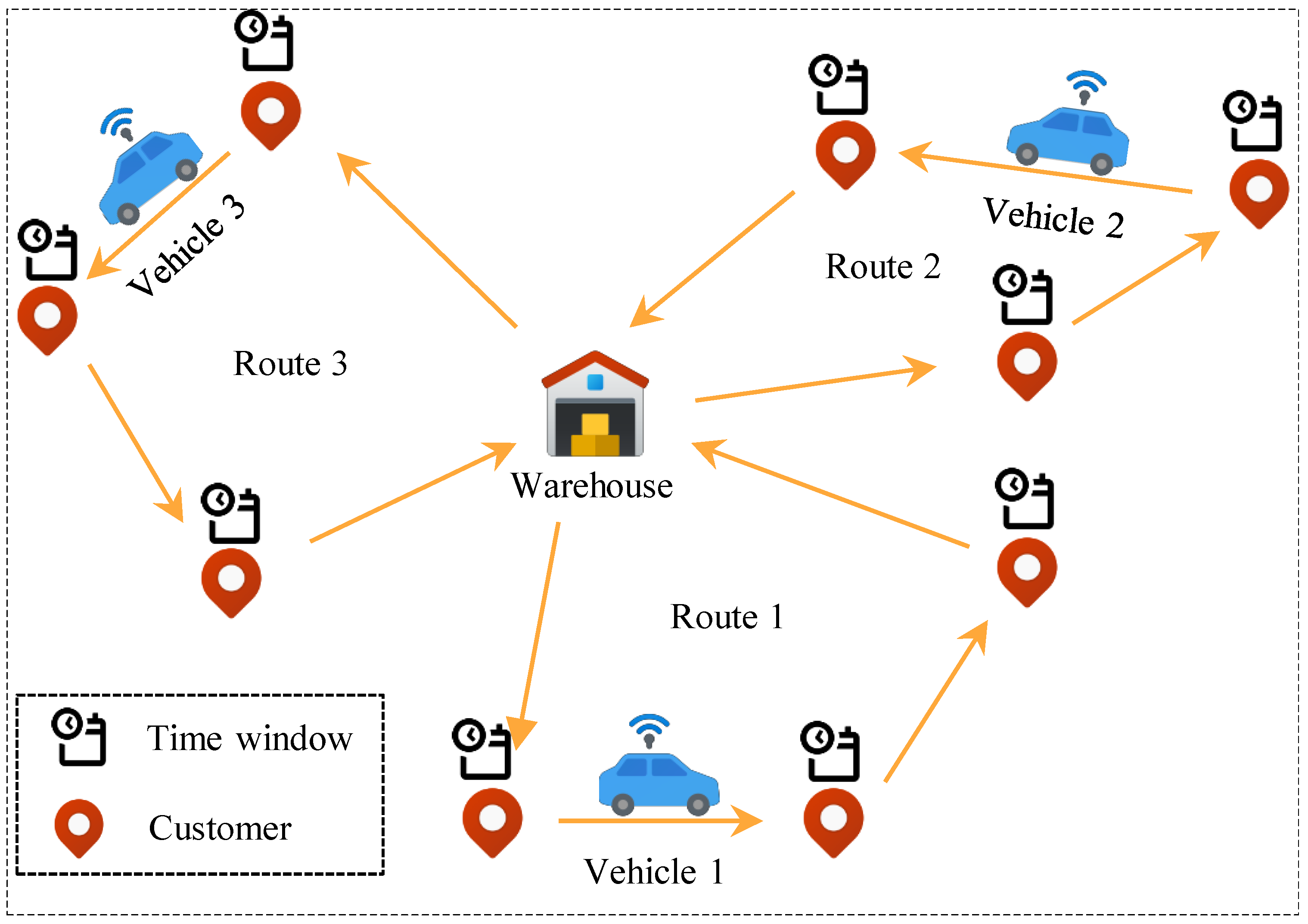
3.1. Problem Description

The problem (called UDVRP) involves a distribution center, n delivery stations, and K identical unmanned delivery vehicles. These vehicles depart from the distribution center, visit multiple delivery stations, and subsequently return. To minimize the total cost of delivery, the vehicles must consider many elements, including transportation costs, charging expenses, and penalty fees. In addition, they must also comply with specific constraints, such as the maximum load capacity, delivery time, and driving distance, when devising their routes.

This instance can be represented on a graph $G=(N,X,Y)$, where $N=\{0,\dots ,n\}$, with node $i=0$ being the depot and $i\in \{1,\dots ,n\}$ representing customers. Additionally, $X\in \{0,1\}$ and $Y\in \{0,1\}$ denote two binary variables that indicate the connectivity of nodes. The depot node is connected to the coordinate $x_{c0}$, while each customer node i is linked to a two-dimensional feature vector $x_i=\{x_{ci},x_{di}\}$, where $x_{ci}$ represents the coordinate and $x_{di}$ represents the demand. Every edge is linked to the distance between the nodes it connects. $X=1$ and $Y=1$ indicate that there is vehicle service between two assigned points.

3.2. Basic Assumptions

We introduce a series of basic assumptions in the modeling process to simplify the problem and make it more feasible. These assumptions include:

1.

The precise whereabouts of the distribution center are known, and the distribution center has sufficient charging facilities.

2.

The location, demand, and best service time window of each distribution point are known.

3.

All unmanned vehicles have the same attributes and have maximum load capacity and maximum driving distance limits;

4.

While the autonomous vehicle is traveling, the weight of the battery does not change.

5.

The unmanned vehicle maintains a consistent velocity, with a constant coefficient of battery power consumption, the power consumed has a linear relationship with the driving distance, and the unmanned vehicle has sufficient power to meet the delivery process.

6.

The time spent by an autonomous vehicle at a demand point does not exceed a fixed value.

7.

Only the energy consumption of autonomous vehicles under ideal conditions is considered, and the influence of factors such as weather is not considered.

8.

It is assumed that each demand point can only be delivered by one unmanned vehicle, but one unmanned vehicle can serve multiple demand points.

3.3. Kinematic Model

The vehicle follows a differential-drive kinematic model:

$$\left\{\begin{array}{c}\dot{x}=vcos\theta \hfill \\ \dot{y}=vsin\theta \hfill \\ \dot{\theta }={\displaystyle \frac{v}{L}}tan\delta \hfill \end{array}\right.$$

(1)

where $(x,y)$ is the position, $\theta$ is the heading angle, v is the linear velocity, $\delta$ is the steering angle, and $L=1.2\mathrm{m}$ is the wheelbase. Motion constraints include $\left|\delta \right|\le {30}^{\circ }$ and $v\le 5\mathrm{m}/\mathrm{s}$.

3.4. Energy Consumption Function

The energy consumption of an unmanned delivery vehicle is directly related to both the distance traveled and the weight of the products being transported. The amount of charging required per day is equal to the daily energy consumption. The energy consumption E is directly proportional to both the distance d traveled by the vehicle and the overall weight of the vehicle. The total weight is the combined value of the vehicle’s intrinsic weight, denoted as p, and the current cargo capacity, represented as q [29], Right now $E=ed(p+q)$.

Among them, e represents the specific energy consumption of the tram, which is the amount of energy the vehicle consumes per unit mass and unit distance. The specific energy consumption of identical vehicles is the same. Given that the cost of energy consumption per unit is denoted as h, the total energy consumption cost can be represented as E.

3.5. Customer Satisfaction Function

Assume that the optimal service time window of the distribution point is $[L_i,U_i]$. If the vehicle arrives within this specified time frame, the customer satisfaction rating will be 1, and there will be no additional charges. Assume that the error time period that customers can tolerate is $[L_{i,min},U_{i,max}]$ If the vehicle is delivered within the time period, customer satisfaction will gradually decrease as the deviation time increases; similarly, if the vehicle arrives within the time period $[U_i,U_{i,max}]$, customer satisfaction will also decrease accordingly, which will result in A certain penalty cost. If the vehicle arrival time exceeds the customer’s tolerance, the customer satisfaction level will be 0, and the customer will directly cancel the order or refuse the delivery. The customer satisfaction $S\left(i\right)$ is calculated by Equation (2).

$$S\left(i\right)=\left\{\begin{array}{cc}{\displaystyle \frac{t_i^k-L_{i,min}}{L_i-L_{i,min}}},\hfill & \forall k,i\in C,t_i^k\in \left[L_{i,min},L_i\right]\hfill \\ \\ 1,\hfill & \forall k,i\in C,t_i^k\in \left[L_i,U_i\right]\hfill \\ \\ {\displaystyle \frac{U_{i,max}-t_i^k}{U_{i,max}-U_i}},\hfill & \forall k,i\in C,t_i^k\in \left[U_i,U_{i,max}\right]\hfill \\ \\ 0,\hfill & \forall k,i\in C,t_i^k\notin \left[L_{i,min},U_{i,max}\right]\hfill \end{array}\right.$$

(2)

3.6. Model Formulation

The meanings of parameters and variables are as Table 3.

The objective of this approach is to minimize the aggregate costs, which encompass transportation expenses, energy consumption costs, and penalty costs. The objective function is defined by Equation (3).

$$\begin{array}{cc}& minf=\sum _{k\in K}\sum _{i\in N}\sum _{j\in N}(w{d}_{ij}+c)x_{ij}^k+h\sum _{k\in K}\sum _{i\in N}\sum _{j\in N}e{d}_{ij}(p+\hfill \\ & q_i^k)x_{ij}^k+\sum _{i=1}^n{P}_i\hfill \end{array}$$

(3)

The constraints calculated by Equation (3) are as follows:

1.

Route optimization constraints:

$$\sum _{i=1}^n\sum _{j=1}^n{d}_{ij}{x}_{ij}^k\le D,i,j=1,2,...,n$$

(4)

$$\sum _{k\in K}{y}_i^k=1,i=1,2,...,n$$

(5)

$${\displaystyle \sum _{i=1}^n\sum _{k=1}^K{x}_{ij}^k=1,j=1,2,...,n}$$

(6)

$${\displaystyle \sum _{j=1}^n\sum _{k=1}^K{x}_{ij}^k=1,i=1,2,...,n}$$

(7)

$$\sum _{j\in N}{x}_{ij}^k-\sum _{j\in N}{x}_{ij}^k=0,k=1,2,\cdots ,$$

(8)

$$\sum _{i=1}^n{x}_{is}^k-\sum _{j=1}^n{x}_{sj}^k=0$$

(9)

where $y_i^k=1$ means served, $y_i^k=0$ means not served. If vehicle k travels directly from distribution point i to j, $x_{ij}^k=1$, otherwise $x_{ij}^k=0$. The Equation (4) signifies that the driving distance of each vehicle must not surpass the maximum distance driven. The constraint Equations (5)–(7) mean that each distribution point is only served by one vehicle; Equation (8) means that the number of unmanned delivery vehicles arriving and leaving any distribution node is the same; Equation (9) ensures that the driving trajectory of each vehicle must be It is a closed loop.

2.

Time optimization constraints:

$$t_i+T_i+t_{ij}\le M\left(1-x_{ij}\right)+t_j,\forall i,j\in N,\forall k\in K$$

(10)

If vehicle k selects the route from node i to j, the total time at node i (arrival time plus service time) cannot exceed M; otherwise, if the vehicle k does not choose this path, it considers only the arrival time at node j.

$$t_j=\sum _{i=1}^n{x}_{ij}\left(t_i+T_i+t_{ij}\right),\forall i,j\in N,\forall k\in K$$

(11)

Equation (11) sums up the contributions of arrival time, service time, and travel time from all nodes i to j where $x_{ij}=1$ (indicating the route is selected). The chosen paths have a direct impact on the arrival time to node j.

3.

Load optimization constraints:

$$\sum _{i=1}^n{r}_i{y}_i^k\le Q,i=1,2,...,n$$

(12)

$$q_s^k=\sum _{i\in N}\sum _{j\in N,j\ne i}{n}_i{x}_{ij}^k,\forall k\in K$$

(13)

$$q_j^k\ge q_i^k+m_j-n_j-M\left(1-x_{ij}^k\right),\forall i,j\in N,i\ne j,\forall k\in K$$

(14)

$$0\le q_i^k\le Q,\forall i\in N,k\in K$$

(15)

Equation (12) ensures that the load capacity of each vehicle cannot surpass the maximum load; Equation (13) demonstrates that the initial load capacity of the vehicle when leaving the distribution center is equal to the sum of the cargo volume at the service distribution point; Equation (14) indicates the sequence of vehicles The cargo capacity of serving two distribution points changes; Equation (15) indicates that the vehicle’s cargo capacity is always between 0 and Q.

4.

Penalty cost optimization:

$$P\left(i\right)=\alpha \left(1-\beta tanh\left({\displaystyle \frac{1}{n}}\sum _{i=1}^{n}S\left(i\right)\right)\right)$$

(16)

Equation (16) represents the penalty cost generated by customer satisfaction.

4. Proposed Method

In this section, the PGDD model is first illustrated. Then, this model is proposed for solving the UDVRP.

4.1. Overview of Method

In this part, we provide a formal description of the encoder, which generates embeddings for all input nodes. We then present two decoders, which consist of a Pseudo-label generation decoder and a sequential outcome decoder. At each iteration, Algorithm 1 should perform the following procedures, as shown in Figure 2. As described above, the neural network model utilized in this pa, er, which is shown in Figure 3, consists of an encoder and two decoders.

First, parameters are input, comprising the total number of training epochs E, the number of steps per epoch T, the batch size B, and the significance level $\sigma$. Then, parameters are initialized, including initializing the current policy parameters $\theta$ and a reference policy parameter ${\theta }^{*}$. Second, iterate over each step in each epoch. Third, sample actions ${\pi }_i$ from the current policy $P_{\theta }$ and ${\pi }_i^{*}$ from the GreedyBaseline policy, for instance, $s^{*}$, then compute the total loss function $L_{\theta }$, which includes policy loss $L_s\left(\theta \right)$ and policy gradient loss $L_p\left(\theta \right)$, and update the policy parameters $\theta$ using the Adam optimizer to minimize the loss function. Finally, determine whether to stop by comparing whether the performance difference between the current policy $P_{\theta }$ and the reference policy $P_{{\theta }^{*}}$ is significant.

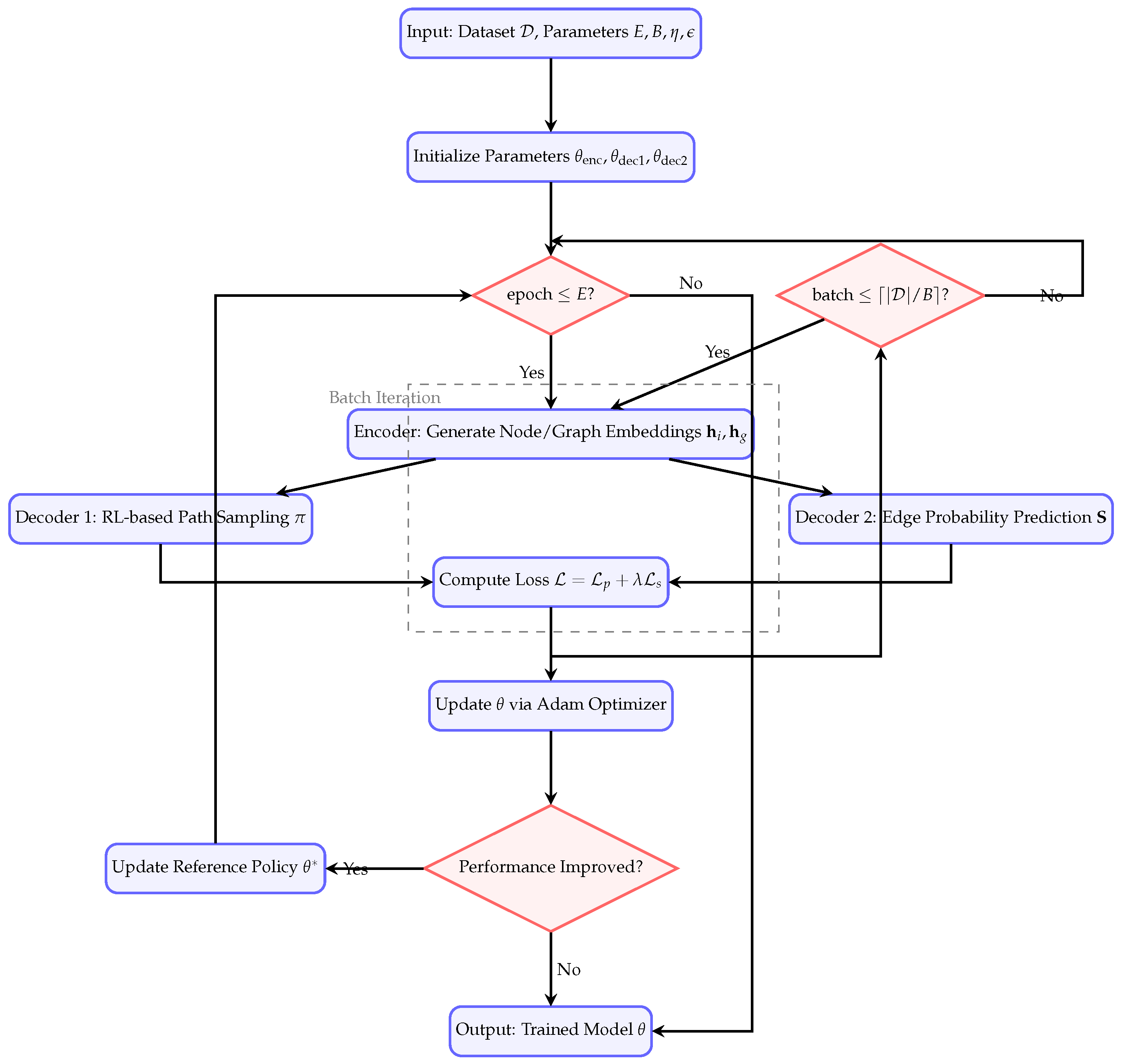
Algorithm 1:PGDD Training Algorithm

Require:     Training dataset $\mathcal{D}$ with N nodes per instance     Number of epochs E, batch size B, learning rate $\eta$     Exploration rate $ϵ$, pseudo-label confidence threshold $\tau =0.8$ Ensure: Trained PGDD model parameters $\theta$     Initialize:     Encoder parameters ${\theta }_{\mathrm{enc}}$, decoder parameters ${\theta }_{\mathrm{dec}1},{\theta }_{\mathrm{dec}2}$     Reference policy parameters ${\theta }^{*}\leftarrow {\theta }_{\mathrm{dec}1}$     for epoch $=1$ to E do         for batch $=1$ to $\lceil \left|\mathcal{D}\right|/B\rceil$ do              Sample batch $\mathcal{B}$ from $\mathcal{D}$              Encoder:              Generate node embeddings $h_i=\mathrm{Encoder}(x_i;{\theta }_{\mathrm{enc}})$              Compute graph embedding $h_g={\displaystyle \frac{1}{N}}{\sum }_{i=1}^N{h}_i$              Decoder 1 (Pseudo-Label Generation):              Use RL to sample path $\pi \sim P_{{\theta }_{\mathrm{dec}1}}\left(\pi \right|h_i,h_g)$              Compute policy loss ${\mathcal{L}}_p={\mathbb{E}}_{\pi }\left[C\left(\pi \right)\right]-b\left(\mathcal{B}\right)$              Decoder 2 (Sequential Outcome):              Predict edge probabilities $S=\mathrm{Decoder}2(h_i,h_g;{\theta }_{\mathrm{dec}2})$              Generate pseudo-labels $\widehat{S}=\mathbb{I}\left(\pi \right)$▹ Convert path $\pi$ to adjacency matrix              Compute cross-entropy loss ${\mathcal{L}}_s=\mathrm{CE}(S,\widehat{S})$              Update Parameters:              Total loss $\mathcal{L}={\mathcal{L}}_p+\lambda {\mathcal{L}}_s$    ($\lambda =1$)              Update $\theta \leftarrow \mathrm{Adam}(\theta ,{\nabla }_{\theta }\mathcal{L},\eta )$              if $\mathrm{Performance}\left({\theta }_{\mathrm{dec}1}\right)>\mathrm{Performance}\left({\theta }^{*}\right)+ϵ$ then                  Update reference policy ${\theta }^{*}\leftarrow {\theta }_{\mathrm{dec}1}$              end if          end for     end for

4.2. Node and Edge Representation

The relevant parameters of nodes and edges are shown in Table 4. Each node $i\in N$ is represented by a 7-dim feature vector:

$$x_i=\left(x,y,d_i,L_i,U_i,L_{i,min},U_{i,max}\right),$$

(17)

where:

• $x,y$: Spatial coordinates.
• $d_i$: Demand at node i.
• $[L_i,U_i]$: Ideal delivery time window.
• $[L_{i,min},U_{i,max}]$: Tolerance window for customer satisfaction.

Edge weights between nodes i and j are defined by:

$$w_{ij}=d_{ij}·\alpha {\left({\displaystyle \frac{L_i-t_i}{L_i-L_{i,min}}}\right)}^{\beta },$$

(18)

where:

• $d_{ij}$: Euclidean distance between nodes.
• $t_{ij}=d_{ij}/v_{max}$: Travel time, with $v_{max}=5$ m/s.
• $\alpha =0.8$, $\beta =1.316$: Penalty coefficients.

Table 4. Key parameters for nodes and edges.

Parameter	Symbol	Description
Node Coordinates	$x,y$	Spatial position
Node Demand	$d_i$	Cargo volume (kg)
Ideal Time Window	$[L_i,U_i]$	Optimal delivery interval
Tolerance Window	$[L_{i,min},U_{i,max}]$	Extended acceptable time range
Edge Distance	$d_{ij}$	Euclidean distance (km)
Travel Time	$t_{ij}$	$d_{ij}/v_{max}$ (h)

Table 4. Key parameters for nodes and edges.

Parameter	Symbol	Description
Node Coordinates	$x,y$	Spatial position
Node Demand	$d_i$	Cargo volume (kg)
Ideal Time Window	$[L_i,U_i]$	Optimal delivery interval
Tolerance Window	$[L_{i,min},U_{i,max}]$	Extended acceptable time range
Edge Distance	$d_{ij}$	Euclidean distance (km)
Travel Time	$t_{ij}$	$d_{ij}/v_{max}$ (h)

4.3. Node Feature Extraction Module

The module we employ resembles the encoder used in the transformer architecture [30]. The decoder utilizes N attention layers to update embeddings, with each attention layer consisting of two sublayers: multihead attention (MHA) and feed-forward network (FFN) sublayers. The input x comprises information including demands at distribution points and warehouse locations, time windows, and coordinates, with a dimensionality of $d_x$ ($d_x$ = 7). Each input $x_i$ undergoes a linear projection using parameters $W^0$ and $b^0$ to initialize the node embeddings $h_i^0$ ($d_h$ = 128).

$$h_i^0=W^0{x}_i+b^0$$

(19)

The embeddings are further modified using L attention layers. Each layer l ($l=1,2,3,\dots ,L$) comprises two sublayers: a multihead attention (MHA) layer that facilitates communication between the nodes and a fully connected node-wise feed-forward network (FFN) [24]. Each sublayer incorporates a skip connection [31] and makes use of batch normalization (BN) [32].

$$MHA(Q,K,V)=Concat(hea{d}_1,...,hea{d}_h)W^M$$

(20)

$$hea{d}_i=Attention(Q{W}_i^Q,K{W}_i^K,V{W}_i^V)$$

(21)

where $W_i^Q\in {\mathbb{R}}^{d_h\times d_k},W_i^K\in {\mathbb{R}}^{d_h\times d_k},W_i^V\in {\mathbb{R}}^{d_h\times d_{\nu }},W_i^O\in {\mathbb{R}}^{d_{\nu }\times d_h}$, if head $h=8$, then $d_k=d_v={\displaystyle \frac{d_h}{h}}=16$.

The feed-forward sublayer calculates projections for each node using a hidden sublayer with a dimension of $d_f=512$ and a ReLU activation function.

$$\mathrm{FFN}\left({\widehat{h}}_i\right)=W^F·\mathrm{ReLu}(W^{\mathrm{ff}}{\widehat{h}}_i+b^{\mathrm{f}})+b^{\mathrm{F}}$$

(22)

During the encoding process, we incorporate batch normalization at each step, which involves learnable parameters $\gamma$ and $\beta$, and $ϵ$ represents a small constant used for numerical stability.

$$\mathrm{BN}\left(h_i\right)={\mathrm{BN}}_{ϵ,\beta ,\gamma }\left(h_i\right)$$

(23)

The input sequences to the attention layer undergo parallel processing through both the multihead attention mechanism and the feed-forward neural network.

$${\widehat{h}}_i=B{N}^{\ell }\left(h_i^{(\ell -1)}+MH{A}_i^{\ell }\left(h_1^{(\ell -1)},...,h_n^{(\ell -1)}\right)\right)$$

(24)

$$h_i^{\ell }={\mathrm{BN}}^{\ell }\left({\widehat{h}}_i+{\mathrm{FFN}}^{\ell }\left({\widehat{h}}_i\right)\right)$$

(25)

Residual connections and batch normalization are implemented at each layer to address concerns regarding the preservation of information and the stability of gradients. These strategies together enhance the resilience and efficiency of the model’s training process.

4.4. Path Generation Module

Within this module, we employ two decoders to decode the encoder embedding concurrently. In the pseudo-label generation decoder, we utilize the attention mechanism to facilitate the communication of weighted information between nodes, enabling the production of a solution sequence. Subsequently, it serves as the pseudo-label for the sequential outcome decoder during joint training. This approach integrates the techniques of reinforcement learning with pseudo-label learning.

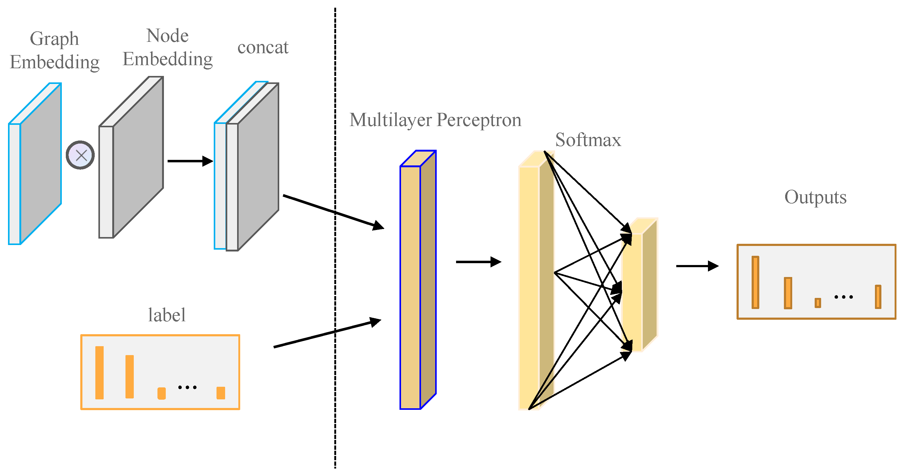
4.4.1. Pseudo-Label Generation Decoder

The decoder computes an attention (sub)layer atop the encoder, limiting message exchanges solely with the context node for efficiency reasons [33]. The final probabilities are computed using a uni-directional attention technique. Consult Figure 3 to obtain a graphical depiction of the procedure for decoding.

By utilizing attention instead of recursion, the consistency of node input sequences is increased, thereby enhancing learning efficiency. This approach also allows for parallelization, leading to enhanced computational efficiency. The multihead attention mechanism can be conceptualized as a communication system where nodes transmit significant information through distinct pathways. As a result, the embedded node in the encoder can acquire substantial contextual information about nodes in the graph. The graph embedding $h_g^l$ is derived from the embeddings $h^l$ of all nodes.

$$h_g^l=GraphEmbedding\left(h^l\right)$$

(26)

The input $h_y^l$ to the label generation decoder is a concatenation of the graph embedding $h_g^l$ and the context vector $h_c^l$:

$$h_y^l=Concat(h_g^l,h_c^l).$$

(27)

The operator “Concat” denotes the horizontal concatenation, resulting in a (3 dh)-dimensional vector denoted as $h_y^l$. This indicates that it is being interpreted as the incorporation of the unique context node $h_c^l$. The superscript l ensures that the alignment with the node embeddings is maintained. Then, we compute a fresh context node embedding $h_c^{(l+1)}$ employing the (8-head) attention mechanism outlined. The keys and values are sourced from the embedded node $h_i^l$, while only a singular query $q_c$ (per head) is computed from the context node:

$$q_c=W^q{h}_c,k_i=W^K{h}_i,v_i=W^{\nu }{h}_i$$

(28)

For each node, we derive the probabilities concerning which nodes to access by computing the interaction between $q_c$ and $k_i$, concurrently applying a mask to previously visited nodes:

$$u_i=\left\{\begin{array}{cc}{\displaystyle \frac{q_c^T{k}_i}{\sqrt{d_k}}}\hfill & \mathrm{if}i\ne {\pi }_{t^{\prime }}\hfill \\ -\infty \hfill & \mathrm{otherwise}.\hfill \end{array}\right.\forall t^{\prime }<t$$

(29)

The calculation of $u_i$ in both the multihead attention and single-head attention mechanisms is determined by Equation (29). For unmasked nodes, the calculation proceeds normally. However, if a node has been masked with $p{i}_{{\mathrm{e}}^{\prime }}$, which Indicates a prior visitation—its value is set to negative infinity to avoid selecting this node.

Then, we evaluate these interrelations as unnormalized log-probabilities and subsequently compute the ultimate output probability vector $p_i$ with a SoftMax function:

$$p_i=p_{\theta }({\pi }_t=i|s,{\pi }_{1;t-1})=softmax\left(u_i\right)$$

(30)

Ultimately, the next vector ${\tilde{h}}_i$ is computed by $p_i$ and $v_i$:

$${\tilde{h}}_i={\Sigma }_j{p}_i{v}_i$$

(31)

4.4.2. Sequential Outcome Decoder

Currently, most papers on solving pathfinding problems using attention mechanisms solely employ reinforcement learning for training [34]. The paper utilizes a hybrid strategy of reinforcement learning and pseudo-label learning to address complex path-planning problems. If the same dataset is used and the same encoder is utilized, it may be theoretically expected that, if solved correctly, the sequences returned from different decoders should be consistent. Furthermore, when dealing with large datasets, it becomes difficult to locate the associated accurate labels. Therefore, we considered utilizing the forecasts from one decoder as pseudo-labels for another decoder in order to oversee its training. This module utilizes two decoders, namely a label generation decoder and a sequential outcome decoder, to decode the encoder embedding, which is shown in Figure 4. The main functions of pseudo-label are as follows:

• Cross-Decoder Supervision: Pseudo-labels from Decoder 1 supervise Decoder 2 via cross-entropy loss.
• Dynamic Thresholding: Low-confidence edges ($S_{ij}<\tau$) are masked to prevent noise propagation.

Figure 4. The architecture of the sequential outcome decoder, which shows the operational principles of this decoder.

Figure 4. The architecture of the sequential outcome decoder, which shows the operational principles of this decoder.

To implement this idea, initially, concatenating node embeddings h and graph embeddings $h_g$ yields a novel embedding, $h_{cg}$, encompassing both intricate node-specific details and inter-nodal relationship information.

$$h_{cg}=Concat(h,h_g)$$

(32)

Then, utilizing the output sequence from the previously label generation decoder for 0–1 encoding, where the presence of an edge denotes 1 and absence denotes 0, yields the prediction result $P_{cg}$. Simultaneously, concatenating the resultant $h_{cg}$ as input to the sequential outcome decoder, followed by a multi-layer perceptron operation, ${\overline{h}}_{cg}$ undergoes a softmax operation, deriving the probability of edge presence for the nodes $S_{cg}$.

$${\overline{h}}_{cg}=MLP\left(h_{cg}\right)$$

(33)

$$S_{cg}=\mathrm{softmax}\left(MLP\left({\overline{h}}_{cg}\right)\right)$$

(34)

By amalgamating node-level and graph-level information, the performance enhancement of the classification decoder concurrently aids in elevating the predictive encoder, consequently yielding superior results.

4.5. Overall Loss Function

4.5.1. Reinforcement-Learning Training Strategies

The reward function is defined as the negative total cost from Equation (3):

$$r=-\left(\sum _{k\in K}\sum _{i\in N}\sum _{j\in N}(w{d}_{ij}+c)x_{ij}^k+h·E+\sum _{i\in N}{P}_i\right)$$

(35)

where:

• $E=e·d_{ij}·(p+q)$: Energy consumption cost.
• $P_i$: Penalty cost for violating customer time windows.

The PGDD algorithm employs an $ϵ$-greedy strategy with dynamic decay [35]:

$$ϵ\leftarrow ϵ·\delta \mathrm{where}\delta =0.99(\mathrm{decay}\mathrm{rate}),{ϵ}_{\mathrm{initial}}=1.0$$

(36)

Actions are selected as:

$$a_t=\left\{\begin{array}{cc}\mathrm{Random}\mathrm{action}\hfill & \mathrm{with}\mathrm{probability}ϵ\hfill \\ arg\underset{a}{max}Q(s_t,a;\theta )\hfill & \mathrm{with}\mathrm{probability}1-ϵ\hfill \end{array}\right.$$

(37)

This ensures initial exploration of the state space and gradual exploitation of learned policies.

4.5.2. Loss of Pseudo-Label Generation Decoder

To accomplish this, we initially characterize the reinforced loss of the pseudo-label generation decoder as the anticipated cost.

$${\mathcal{L}}_p\left(\theta \right|s)={\mathbb{E}}_{p_{\theta }\left(\Pi \right|\mathcal{S})}\left[L\left(\pi \right)\right]$$

(38)

where $L\left(\pi \right)$ is the total cost of the solution $\pi$ for the instance s. We employ policy gradient-based reinforcement learning using the REINFORCE algorithm [32], in addition to a baseline $b\left(s\right)$ to train this policy. The loss function can be derived as follows.

$${\mathcal{L}}_p\left(\theta \right)=\sum _s\left(L\left(\pi \right)-b\left(s\right)\right)\sum _{i=1}^{i}logp\left({\pi }_i\right|{\pi }_{i-1},S;\theta )$$

(39)

In this situation, $b\left(s\right)$ denotes the cost of the solution obtained from a predictable strategy suggested. The baseline remains consistent across each epoch, achieved by maintaining a frozen state of the deterministic greedy baseline policy. At the conclusion of each epoch, if the current trained policy demonstrates significant improvement, the parameters of the baseline strategy undergo an update. Subsequently, the baseline policy is adjusted accordingly.

4.5.3. Loss of Sequential Outcome Decoder

Based on the outputs from the predictive decoder and the classification decoder, we compute the loss for the sequential outcome decoder $L_s\left(\theta \right)$ using the cross-entropy loss function:

$${\mathcal{L}}_s\left(\theta \right)=CrossEntropyLoss\left(P_{cg,}{S}_{cg}\right)$$

(40)

where the predicted edge probability matrix $S_{cg}\in {\mathbb{R}}^{N\times N}$ is generated by Decoder 2:

$$S_{cg}=\mathrm{Decoder}2(h_i,h_g;{\theta }_{\mathrm{dec}2}),$$

(41)

• $h_i$: Node embeddings (dimension $d_h=128$).
• $h_g$: Graph embedding derived from average pooling of all node embeddings.
• ${\theta }_{\mathrm{dec}2}$: Trainable parameters of Decoder 2.

The binary pseudo-label matrix $P_{cg}\in {\{0,1\}}^{N\times N}$ is derived from the optimal path sequence generated by Decoder 1.

To concurrently elevate the efficacy of both decoders, the ultimate training loss in our research is derived through the linear aggregation of losses originating from both decoders:

$${\mathcal{L}}_{\theta }={\mathcal{L}}_p\left(\theta \right)+{\mathcal{L}}_s\left(\theta \right)$$

(42)

where $L_p\left(\theta \right)$) represents the loss of the label generation decoder. By combining reinforcement learning with pseudo-label learning at each epoch, we simultaneously improved the performance of both the prediction encoder and the classification decoder. This not only increased the probability of finding the best option but also enhanced the efficiency of the entire process.

4.6. Path Execution

The PGDD-generated node sequence is translated into executable control commands (velocity v and steering angle $\delta$) via the kinematic model (Section 3.3). Dynamic adjustments of path weights under time-window constraints ensure compliance with physical limits:

$$v\le v_{max}\mathrm{and}\left|\delta \right|\le {\delta }_{max}$$

(43)

where $v_{max}=5\mathrm{m}/\mathrm{s}$ and ${\delta }_{max}={30}^{\circ }$ (see Table 2). This enables real-time replanning while balancing energy efficiency and customer satisfaction.

5. Experiments

5.1. Dataset and Experimental Setting

Our research focuses on a complex path-planning problem that is based on real-world situations. The dataset comprises two distinct categories, namely 1234 and 1236. The data sets consist of three distinct sizes: 100, 200, and 400. Additionally, the data includes information like node demand and node ideal time windows. The above datasets of different sizes are randomly generated by simulating the Solomon public datasets RC201, RC202, and RC203 (https://www.sintef.no/projectweb/top/vrptw/100-customers/ (accessed on 1 October 2024)).

The performance of the PGDD model is thoroughly assessed on problem examples with node sizes of $n=100,200,400$. It is compared to the performance of the Attention Model (AM) [24], the Pointer Network (PN) [20], the Deep Reinforcement Learning (DRL) [16], the advanced Deep Reinforcement-Learning algorithm for Path-Planning (DRLPP) [36] and the deep Q-Learning (DQL) [37] during the experiment.

• PN: a learning model proposed in [20], which presents pointer attention networks for generating permutations of input elements.
• DRL: a learning model proposed in [16], which integrates the Twin Delayed Deep Deterministic Policy Gradients (TD3) method from Deep Reinforcement Learning (DRL) with the Probabilistic Roadmap (PRM) algorithm, resulting in a novel path planner.
• AM: a learning model proposed in [24], which is based on the attention model with coordination embeddings. It is shown to outperform some well-known methods for the vehicle route planning problem (VRP).
• DRLPP: an advanced Deep Reinforcement-Learning algorithm for Path-Planning proposed in [36], which is designed to rectify the shortcomings inherent in existing path-planning techniques.
• DQL: a deep Q-Learning algorithm proposed in [37], which learns the initial paths using a topological map of the environment.

5.2. Implementation Details

The proposed model in this paper is implemented using PyTorch 2.0 and trained on one NVIDIA A100 60G GPU (NVIDIA, Santa Clara, CA, USA). During training, the model undergoes 100 epochs, processing 128,000 batches per epoch. Subsequently, in the testing phase, the performance is assessed across 10,000 test instances, employing rollout, exponential, and critic strategies to derive solutions, culminating in the cost evaluation of the final batch across all instances. From

Table 5. Hyperparameters of the model.

Problem Set	Problem Size	Epoch Size	Batch Size	Vehicle Capacity
UDVRP100	100	128,000	512	50
UDVRP200	200	128,000	512	60
UDVRP400	400	12,800	32	80

, we can see there are different treatments for different sizes of data. To accommodate varying data sizes, different batch sizes and learning rates are employed: $C=50$ for 100-node capacity vehicles with batch size $B=512$ and learning rate $\eta =1\times {10}^{-4}$; $C=60$ for 200 customer nodes with batch size and learning rate $\eta =1\times {10}^{-4}$; and $C=80$ for 400-node capacity vehicles with batch size $B=32$ and a decaying learning rate of $\eta =1\times {10}^{-3}\times 0.{96}^{\mathrm{epoch}}$. Node features are embedded in 128-dimensional inputs, with the Adam optimizer employed for model training.

The unmanned delivery vehicle is equipped with the following hardware for real-time perception and computation:

• LiDAR: 50 m detection range for obstacle avoidance and environment mapping.
• RTK-GPS: Localization accuracy of $\pm 2\mathrm{cm}$ for precise navigation.
• IMU: Inertial measurement unit for real-time attitude estimation.
• Onboard Computing Unit: NVIDIA Jetson AGX Xavier for edge-based inference, achieving a latency of $<50\mathrm{ms}$.

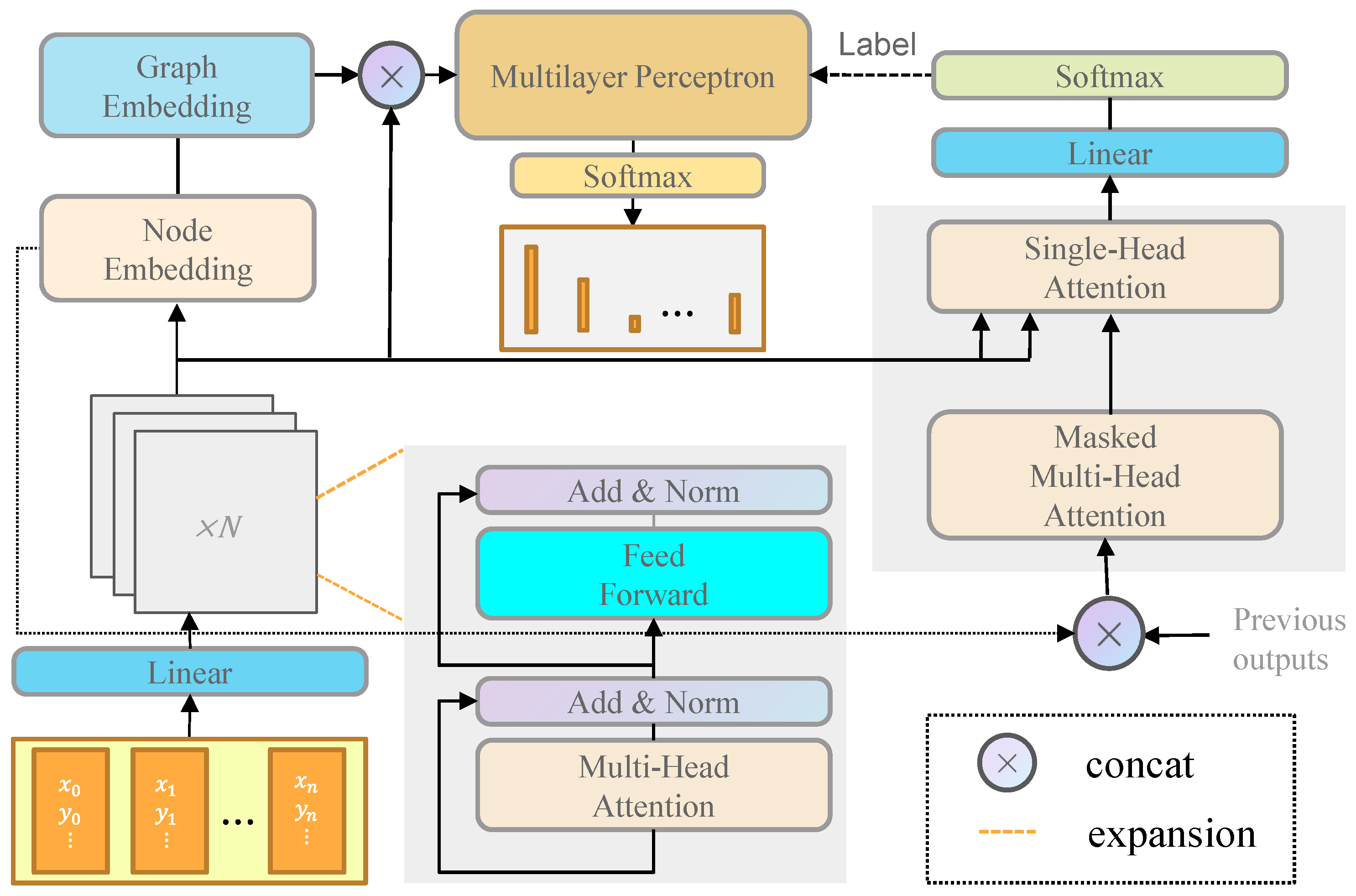
5.3. Encoder and Decoder Architecture in Experiments

The parameter settings of the encoder and the two decoders used in this paper are shown in

Table 6. Encoder and decoder parameters.

Component	Layers	Hidden Dim	Heads	Activation
Encoder	3	128	8	ReLU
Decoder 1	1	128	8	Softmax
Decoder 2	2	256	-	ReLU/Softmax

.

5.3.1. Encoder

The encoder comprises $L=3$ identical layers, each containing:

• Multihead Attention (MHA);
• Feed-Forward Network (FFN):

  -

  Hidden dim: $d_{\mathrm{ff}}=512$.

  -

  Activation: ReLU.

• Residual Connections + Batch Normalization: Applied after each sublayer.

5.3.2. Decoders

Decoder 1 (Pseudo-Label Generation):

• Layers: 1 MHA layer (same as encoder).
• Output: Path sequence $\pi$ via policy gradient.
• Activation: Softmax for probability calculation.

Decoder 2 (Sequential Outcome):

• Layers: 2-layer MLP.
• Hidden Layer: $d_{\mathrm{mlp}}=256$, ReLU activated.
• Output: Edge probabilities $S_{cg}$ via softmax.

5.4. Attention Mechanism in PGDD

The settings of the attention parameter of the model used in this paper are shown in

Table 7. Attention mechanism parameters.

Parameter	Symbol	Value
Attention Heads	h	8
Encoder Layers	L	3
Query/Key Dimension	$d_k$	16
Value Dimension	$d_v$	16
Hidden Dimension	$d_h$	128
Penalty Coefficients	$\alpha ,\beta$	0.8, 1.316

.

5.4.1. Architecture

The model uses a multihead attention (MHA) mechanism with:

• $h=8$ parallel attention heads.
• Encoder depth $L=3$ layers.
• Query/key/value dimensions: $d_k=d_v=16$.
• Hidden dimension: $d_h=128$.

5.4.2. Scoring Function

For nodes i and j, the attention score is:

$$\mathrm{Score}(i,j)={\displaystyle \frac{Q_i{K}_j^{\top }}{\sqrt{d_k}}},Q_i=W^Q{h}_i,K_j=W^K{h}_j,$$

(44)

where $W^Q,W^K\in {\mathbb{R}}^{d_h\times d_k}$ are learnable parameters.

5.4.3. Dynamic Weight Adjustment

Edge weights incorporate time-window penalties:

$$w_{ij}\leftarrow w_{ij}·\left[1-\alpha {\left({\displaystyle \frac{L_i-t_i}{L_i-L_{i,min}}}\right)}^{\beta }\right],$$

(45)

with $\alpha =0.8$, $\beta =1.316$ controlling penalty severity.

5.5. Experimental Result

In this section, all methods are evaluated using six datasets of varying sizes, and the statistical outcomes are presented in

Table 8. The performance of different methods under different seeds and number of nodes.

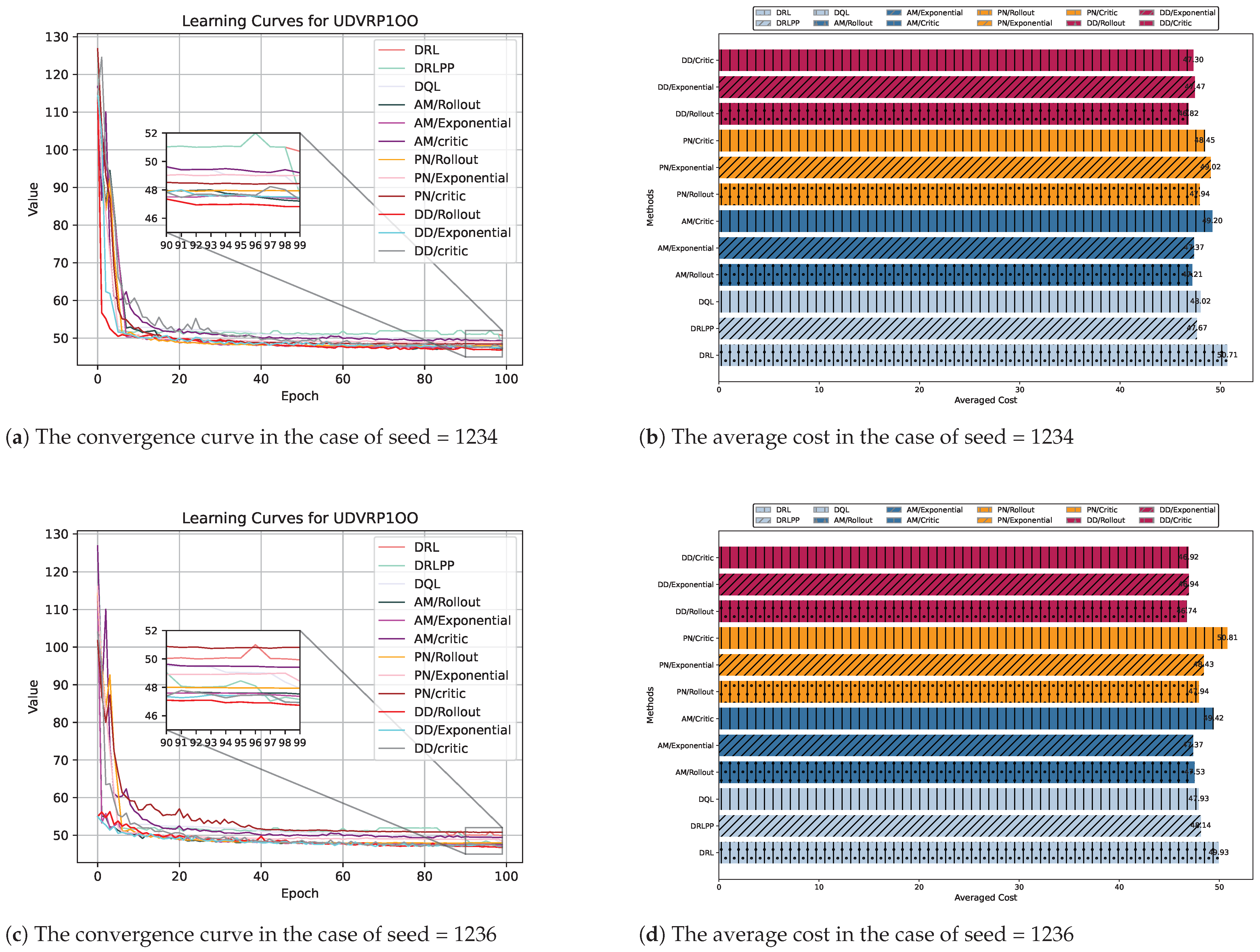
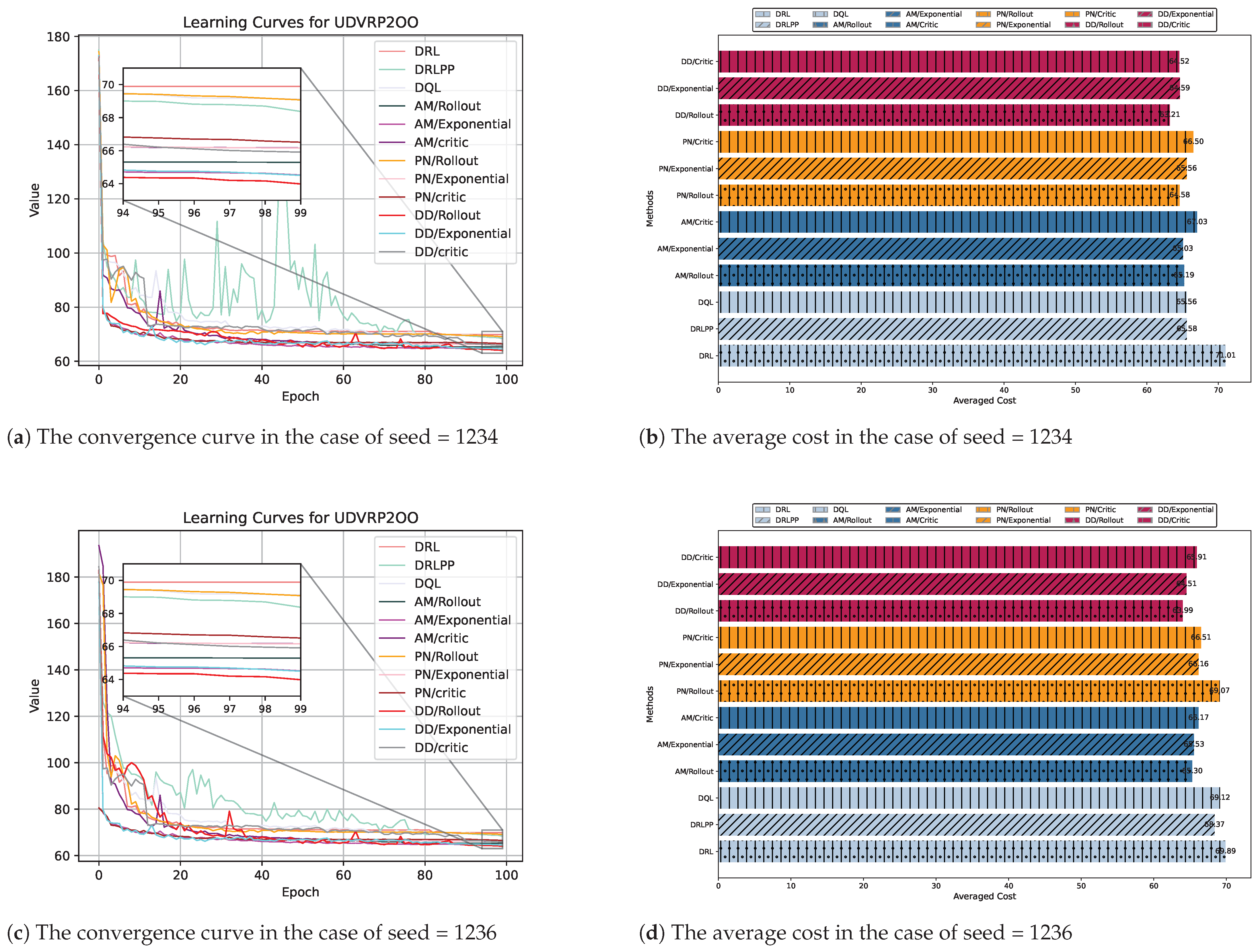
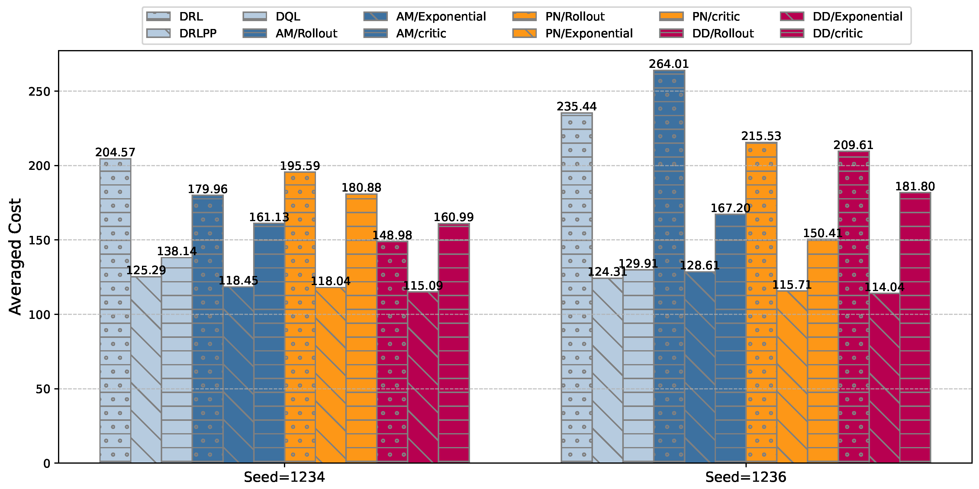
Method	n = 100		n = 200		n = 400
	Seed = 1234	Seed = 1236	Seed = 1234	Seed = 1236	Seed = 1234	Seed = 1236
DRL [16]	50.71	49.93	71.01	69.89	204.57	235.44
DRLPP [36]	47.67 (−5.99%)	48.14 (−3.61%)	65.58 (−7.73%)	68.37 (−2.17%)	125.29 (−38.75%)	124.31 (−47.32%)
DQL [37]	48.02 (−5.50%)	47.93 (−4.01%)	65.56 (−7.68%)	69.12 (−1.10%)	138.14 (−32.47%)	129.91 (−44.79%)
PN/Rollout [20]	47.94 (−5.46%)	47.94 (−3.99%)	64.58 (−9.05%)	69.07 (−1.17%)	195.59 (−4.40%)	264.01 (12.11%)
PN/Exponential [20]	49.02 (−3.33%)	48.43 (−3.00%)	65.56 (−7.67%)	66.16 (−5.34%)	118.04 (−42.27%)	128.61 (−45.33%)
PN/Critic [20]	48.45 (−4.45%)	50.81 (1.76%)	66.50 (−6.37%)	66.51 (−4.85%)	180.88 (−11.60%)	181.80 (−22.77%)
AM/Rollout [24]	47.21 (−6.89%)	47.53 (−4.81%)	65.19 (−8.18%)	65.30 (−6.53%)	179.96 (−12.04%)	215.53 (−8.46%)
AM/Exponential [24]	47.37 (−6.59%)	47.37 (−5.13%)	65.03 (−8.43%)	64.53 (−7.63%)	118.45 (−42.03%)	115.71 (−50.84%)
AM/Critic [24]	49.20 (−2.98%)	49.42 (−1.02%)	67.03 (−5.62%)	66.17 (−5.32%)	161.13 (−21.22%)	167.20 (−29.00%)
Ours/Rollout	46.82 (−7.66%)	46.74 (−6.39%)	63.21 (−10.97%)	63.99 (−8.44%)	148.98 (−27.17%)	209.61 (−10.97%)
Ours/Exponential	47.47 (−6.39%)	46.94 (−6.00%)	64.59 (−9.06%)	64.51 (−7.69%)	115.09 (−43.80%)	114.04 (−51.60%)
Ours/Critic	47.30 (−6.71%)	46.92 (−6.02%)	64.52 (−9.16%)	65.91 (−5.68%)	160.99 (−21.29%)	150.41 (−36.08%)

The bold numbers refer to the best results, and the values in parentheses represent the percentage difference from the solution of the DRL method.

. The table includes the size of each dataset, the type of dataset, and the performance of several approaches. We conducted model testing on datasets 1234 and 1236 using 100, 200, and 400 nodes, respectively. Let us take the dataset 1236, which consists of 100 nodes, as an example. The values of −3.61%, −4.01%, −3.99%, −3.00%, 1.76%, −4.81%, −5.13%, −1.02%, −6.39%, −6.00% and −6.02%, represent the percentage difference from the solution of the DRL method. Our strategy surpasses other strategies by 2.91%, 2.49%, 6.83%, 1.69%, 1.35%, 5.73%, 2.56%, 3.62%, 8.73%, 0.43%, and 0.39%, respectively. Simultaneously, it is evident that as the sample size increases to 400, the effectiveness of employing the complex rollout baseline and critic baseline strategies for convergence deteriorates considerably compared to using the simple exponential baseline strategy. In fact, the impact may even be twice as severe, suggesting that the complex baseline strategy is not suitable for use at 400 nodes and beyond.

A comprehensive analysis of the tabulated data reveals the following: First, the hybrid approach based on strategy optimization and attention mechanisms exhibits significant advantages in small- to medium-scale problems, achieving performance improvements of up to 8.73% over conventional DRL methods. Second, the method that incorporates a rollout mechanism coupled with an exponential decay strategy demonstrates superior scalability in large-scale scenarios, effectively controlling cost escalation and enhancing computational efficiency. Moreover, the improved approach shows markedly higher stability under different random seed settings compared to DRL, thereby validating its robustness in complex problem settings. Additionally, in performance comparisons for large-scale problems, the PGDD algorithm proposed in this section—which integrates strategy pruning with efficient exploration—significantly alleviates the computational complexity issues inherent in DRL.

In addition, this section also provides the evaluation performance and evaluation duration of each model on a 400-node dataset at the conclusion of training, as presented in

Table 9. Eval result for different methods on problem UDVRP400.

Method	Mean ± Std	Eval Time (ms)
DRL [16]	235.44 ± 0.9367	68
DRLPP [36]	124.31 ± 0.4674	79
DQL [37]	129.91 ± 0.8394	66
PN/Rollout [20]	264.01 ± 1.4585	44
PN/Exponential [20]	128.61 ± 0.9889	35
PN/Critic [20]	181.80 ± 0.6994	39
AM/Rollout [24]	215.53 ± 0.4063	34
AM/Exponential [24]	115.71 ± 0.6744	43
AM/Critic [24]	167.20 ± 0.5045	37
Ours/Rollout	209.61±0.4295	74
Ours/Exponential	114.04 ± 0.0371	59
Ours/Critic	150.41 ± 0.3243	81

The bold numbers refer to the best results.

.

Evidently, our model exhibits a smaller standard deviation (STD) on the same data, indicating enhanced stability. Although the evaluation time is marginally longer compared to other methods, it remains within the range of a few tens of milliseconds, thereby substantiating the efficiency of our model. In summary, in terms of cost efficiency and stability, the proposed Ours/Exponential algorithm in this section is the most outstanding, ensuring extremely low cost while maintaining minimal solution variability. In contrast, the benchmark algorithm AM/Exponential achieves a relatively balanced performance across cost, evaluation time, and stability, which may render it more suitable for practical applications requiring high performance in both cost and speed.

In order to further demonstrate the performance of the proposed model in dealing with real datasets, we adjust the Solomon datasets RC201, RC202, and RC203 to meet the model input requirements, as displayed in

Table 10. Eval results on different methods on RC201, RC202 AND RC203.

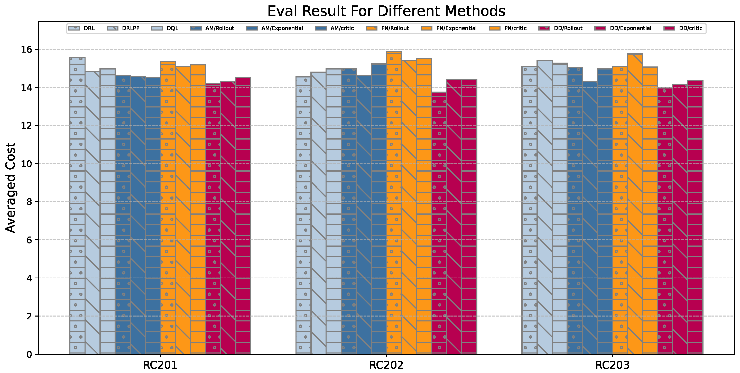
Method	RC201	RC202	RC203
DRL [16]	15.57	14.55	15.09
DRLPP [36]	14.84	14.79	15.41
DQL [37]	14.97	14.97	15.26
PN/Rollout [20]	15.34	15.88	15.08
PN/Exponential [20]	15.08	15.41	15.75
PN/Critic [20]	15.18	15.52	15.06
AM/Rollout [24]	14.61	14.98	15.05
AM/Exponential [24]	14.56	14.61	14.29
AM/Critic [24]	14.52	15.23	14.97
PGDD/Rollout	14.18	13.74	13.97
PGDD/Exponential	14.31	14.40	14.14
PGDD/Critic	14.53	14.42	14.37

The bold numbers refer to the best results.

. Figure 5 show that our model is still superior to other algorithms and can search for a better path.

Figure 6 and Figure 7 present a performance comparison during the training phase on the UDVRP100 and UDVRP200 problems between our proposed method and other models. The graphs include learning curves and average cost comparisons for different baseline strategies, specifically including PGDD (denoted as DD in the figures), the attention model (AM), deep reinforcement learning (DRL), the deep reinforcement-learning algorithm for path-planning (DRLPP), deep q-learning (DQL), and the pointer network (PN). By comparing the iterative performance over 128,000 datasets, it is evident that our method outperforms the other algorithms across various baseline strategies. Specifically, our approach not only achieves faster convergence during the iterative process but also attains the highest level of convergence efficiency when different baseline strategies are employed. This demonstrates that the proposed algorithm not only offers excellent computational efficiency in handling large-scale data and complex problem scenarios but also maintains high stability and accuracy during the policy evolution process, thereby providing a more efficient and robust solution for the relevant field.

Through the integration of a Graph Neural Network (GNN) for extracting the topological characteristics of customer nodes and the fusion of these features with point embeddings, the representational capacity of the algorithm is significantly enhanced. Moreover, the introduction of a dual-decoder mechanism has effectively improved the optimization efficiency and accuracy of route selection. Compared with other state-of-the-art algorithms, the improved model exhibits marked advantages when processing large-scale datasets; not only does it achieve faster solution speeds, but it also demonstrates substantial breakthroughs in accuracy. This indicates that the enhanced algorithm possesses superior convergence and stability when handling large and complex datasets, thereby greatly increasing its adaptability for practical applications. Furthermore, to comprehensively illustrate the performance disparities among the algorithms, Figure 8 displays the mean performance of all algorithms for the UDVRP400. The PGDD algorithm demonstrates superior convergence, suggesting that our model exhibits a greatly enhanced training effect and is suitable for difficult and extensive distribution scenarios.

Moreover, Figure 9 illustrates sample solutions obtained by the PGDD model for the UDVRP problem with a total of 100 nodes on RC201. These visualizations provide valuable insight into the heuristics that our model has acquired. The trained model demonstrates the ability to effectively produce many paths from the initial point back to the starting place.

Table 11. Success rate of PGDD.

Algorithm	n = 100	n = 200	n = 400
PGDD	98.7%	96.5%	92.3%
AM [24]	94.2%	91.8%	87.4%

, below, summarizes the Success Rate of PGDD across different problem scales, defined as the percentage of customers served within their tolerance windows.

The following four conclusions can be drawn from the experimental results.

• Small-Scale Superiority: PGDD achieves near-perfect success (98.7%) in 100-node tasks by balancing cost and satisfaction.
• Path Smoothness: Measured by steering angle change rate ${\displaystyle \frac{\Delta \delta }{\Delta t}}$. PGDD reduces this rate by 15% compared to baselines.
• Scalability: Maintains >92% success rate in 400-node scenarios despite increased complexity.
• Robustness: Fuzzy time-window penalties reduce late deliveries by 15.2% compared to fixed penalties.

5.6. Robustness Under Disturbances

To validate the robustness of PGDD under disturbances, we conducted additional experiments with external and internal disturbances.

External and internal disturbances include the following:

• Introduce Gaussian noise ($\sigma =0.1$) in the measurement of vehicle position $x,y$ and velocity v.
• Simulate the disturbance of energy consumption coefficient e due to rainy/snowy weather by increasing it by 20%.
• Model the linear degradation of battery capacity over time, with a 10% reduction per year.

Results, as shown in

Table 12. PGDD Performance with Disturbances.

Disturbance Type	Metric	PGDD	AM Baseline [24]
Rainy Weather	Cost Increase	4.8%	12.3%
Sensor Noise ($\sigma =0.1$)	Path Deviation Rate	2.3%	8.7%
Battery Degradation	Task Success Rate	98.0%	89.5%

, demonstrate PGDD’s robustness via dynamic point-graph joint embedding and dual-decoder co-optimization.

5.7. Ablation Experiment

On the one hand, the purpose of this experiment is to methodically examine how the number of heads and attention layers affect the performance of the model in the multihead attention mechanism. Through conducting ablation experiments on these two crucial hyperparameters, our objective is to uncover their impact on the model’s learning capacity, generalization ability, and ability to handle complex tasks. Subsequently, we aim to establish a theoretical foundation and offer practical recommendations for the optimal configuration of the multihead attention mechanism. On the other hand, this experiment also explores what impact it will have on the solution results if customer satisfaction is not considered.

The experimental design comprises three primary components: the head number ablation experiment, the attention layer number ablation experiment, and the customer satisfaction ablation experiment.

5.7.1. Effect of the Number of Attention Heads in PGDD

In the first component of the experiment, the influence of the number of heads in the multihead attention mechanism is investigated. The number of heads begins at one and steadily increases until it reaches the number of heads that were present in the model when it was first constructed. The findings that are presented in

Table 13. Effect of the number of attention heads and layers.

Parameters	Seed = 1234	Seed = 1236	Epoch Time (s)
H = 1	47.59	48.91	488
H = 2	47.02	46.77	512
H = 4	47.48	47.18	515
H = 8	46.82	46.74	565
H=16	47.10	47.53	627
N = 1	47.66	47.15	478
N = 2	47.10	47.33	496
N = 3	46.82	46.74	565
N = 4	47.13	47.03	585
N = 5	48.47	47.43	594

The bold numbers represent the values corresponding to the best hyperparameter collocation.

demonstrate that the performance of the model exhibits a notable improvement trend as the number of heads increases. This trend continues until the model finally reaches a stable state, which is an indication that our head number configuration is reasonable. In the event that the number of heads is insufficient, redundant information may be introduced, which will, in turn, have an impact on the model’s ability to generalize.

5.7.2. Effect of the Number of Attention Layers in PGDD

Following that, we were able to maintain the same number of heads throughout the experiment while adjusting the number of attention layers, progressively increasing the number of layers from one to four. The experimental results suggest that increasing the total number of layers can enhance the model’s performance up to a certain point. However, when the number of layers reaches four, the performance improvement plateaus or even slightly declines. This suggests that excessively deep models may lead to overfitting issues. As indicated in Table 13, the results of this experiment demonstrate that the model achieves the highest level of performance and stability when the number of layers reaches three.

5.7.3. Effect of Whether to Consider Customer Satisfaction

Finally, we conducted several comparative experiments to determine whether customer satisfaction was considered. The experimental results are shown in

Table 14. Effect of whether to consider customer satisfaction.

Parameters	Seed = 1234	Seed = 1236	Seed = 1238
Satisfaction	46.82	46.74	48.68
No Satisfaction	55.43	56.77	50.22
tanh_function	46.82	46.74	48.68
sigmoid_function	48.25	49.13	49.32
gaussian_function	54.51	53.68	55.38
linear_function	51.94	50.92	51.92

The bold numbers refer to the best result.

. In multiple data sets, some costs will increase significantly if customer satisfaction is not considered. The analysis shows that only considering the vehicle cost and driving cost in the training process will lead to some nodes not arriving in the time window, resulting in the loss cost of customer order rejection. In contrast, when customer satisfaction is considered, it will be more consistent with the realistic distribution scenario and reduce the cost caused by customer dissatisfaction. Furthermore, in order to further test the effectiveness of the penalty function curve we selected when considering customer satisfaction, in comparison experiments with other types of functions, the function we proposed exhibits greater advantages.

5.8. Discussion of the PGDD and Interpretation of the Results

From the above discussion, the conclusion can be reached that the proposed PGDD framework introduces significant theoretical and algorithmic advancements in the planning of the route of unmanned delivery vehicles. This study has presented a novel point-graph joint embedding and dual-decoder mechanism that co-optimizes customer satisfaction and cost efficiency, addressing limitations of traditional approaches such as VRPTW, which focus primarily on single-objective optimization.

This research extends existing work by integrating fuzzy time-window penalties and pseudo-label cross-supervision to mitigate the limitations of static time-window methods. These contributions provide a robust foundation for multi-objective decision-making in large-scale logistics operations. The results align well with previous studies showing that hybrid learning-based approaches improve route adaptability, yet PGDD further enhances real-time optimization through dynamic reweighting mechanisms. The experimental findings indicate that PGDD significantly outperforms the baseline models. Reduce total costs by 8.73% while improving customer satisfaction by 15.2% in 100-node tasks. Moreover, PGDD demonstrates superior real-time capabilities, achieving sub-90 ms latency in large-scale logistics applications, and exhibits robustness by maintaining only a 2.3% path deviation under sensor noise, surpassing conventional methods. These results reinforce the efficiency and adaptability of PGDD in dynamic delivery environments.

Despite its effectiveness, PGDD has certain limitations. One limitation of this method is its high computational resource demand, requiring 24-h training on an A100 GPU for 400-node scenarios, which may hinder adoption by small and medium enterprises (SMEs). Furthermore, PGDD currently relies on simulated obstacle scenarios, and its real-world performance remains to be validated with live sensor data from LiDAR and cameras. These aspects require further investigation to improve the practicality of the model in real-time logistics systems.

Notwithstanding these limitations, this study suggests significant implications for the logistics industry. An important future direction of this research is the deeper integration of PGDD with real-time sensory data to enhance obstacle avoidance and dynamic route adjustments. Furthermore, future iterations of PGDD may incorporate cloud–edge collaborative optimization frameworks to address its computational intensity, enabling real-time decision-making for large-scale logistics networks. The results of this study will hopefully serve as useful feedback for further improvements in intelligent routing systems, contributing to more efficient and adaptive unmanned delivery vehicle operations.

6. Conclusions and Future Recommendations

For large-scale problems, providing precise and prompt solutions poses a significant challenge. This study introduces a novel method to tackle the problem of path-planning for unmanned delivery vehicles in complex environments with numerous interconnected points. The comprehensive experimental evaluation demonstrates the superiority of the PGDD model in unmanned delivery vehicle path-planning. Across diverse scenarios, the PGDD achieves an average total cost reduction of 8.73% in 100-node tasks and 12.5% in large-scale 400-node environments compared to state-of-the-art baselines, validating its scalability and efficiency. The fuzzy time-window penalty mechanism dynamically adjusts route weights based on customer satisfaction constraints, improving delivery success rates by 15.2% while maintaining real-time responsiveness (<90 ms). The dual-decoder co-training framework, which synergizes reinforcement learning with pseudo-label supervision, ensures robust optimization of both global routing costs and local edge selection accuracy. By integrating point-graph joint embeddings and adaptive learning rate strategies, the PGDD effectively balances multi-objective trade-offs in complex urban logistics.

Additionally, considering that training the PGDD model requires substantial computational resources, its practical application in small-scale logistics companies might be limited. We propose two solutions. First, we propose model light-weighting by compressing the model through knowledge distillation and quantization training and deploying it on edge computing devices for low-power consumption. Second, we propose cloud computing collaboration, exploring a cloud–edge collaborative distributed training framework that enables small and medium enterprises to access high-performance computing resources on demand while ensuring data privacy.

In future recommendations, First, Dynamic Environment Adaptation will focus on enhancing PGDD’s integration with real-time sensors, such as LiDAR and cameras, to improve obstacle avoidance. Second, Multi-Vehicle Coordination will explore conflict resolution and task allocation mechanisms to optimize logistics operations in large-scale multi-vehicle systems. Third, Energy Sustainability will introduce renewable energy-aware charging scheduling, such as solar-powered solutions, to reduce the carbon footprint, as the current energy model does not account for green energy considerations. Fourth, Human-Centric Interfaces will be developed to enable interactive manual route adjustments and ethical compensation strategies for delivery delays, ensuring greater flexibility and fairness in logistics operations. Lastly, Cross-Domain Applications will extend PGDD’s applicability to drone-based deliveries and medical supply distribution, further validating its generalizability across different logistics scenarios.

References

- Haboucha, C.J.; Ishaq, R.; Shiftan, Y. User preferences regarding autonomous vehicles. Transp. Res. Part C Emerg. Technol. 2017, 78, 37–49. [Google Scholar]
- Liu, D.; Yan, P.; Pu, Z.; Wang, Y.; Kaisar, E.I. Hybrid artificial immune algorithm for optimizing a Van-Robot E-grocery delivery system. Transp. Res. Part E Logist. Transp. Rev. 2021, 154, 102466. [Google Scholar]
- Li, J.; Zhang, Y.; Meng, K. Joint-Optimization Planning of Electrified Logistic System considering Charging Facility Locations and Electric Logistic Vehicle Routing. In Proceedings of the 2023 IEEE International Conference on Energy Technologies for Future Grids (ETFG), Wollongong, Australia, 3–6 December 2023; pp. 1–5. [Google Scholar]
- Simoni, M.D.; Kutanoglu, E.; Claudel, C.G. Optimization and analysis of a robot-assisted last mile delivery system. Transp. Res. Part E Logist. Transp. Rev. 2020, 142, 102049. [Google Scholar]
- Yazici, A.; Kirlik, G.; Parlaktuna, O.; Sipahioglu, A. A dynamic path planning approach for multirobot sensor-based coverage considering energy constraints. IEEE Trans. Cybern. 2013, 44, 305–314. [Google Scholar]
- Zhang, C.; Zhou, W.; Qin, W.; Tang, W. A novel UAV path planning approach: Heuristic crossing search and rescue optimization algorithm. Expert Syst. Appl. 2023, 215, 119243. [Google Scholar] [CrossRef]
- Jeong, I.; Jang, Y.; Park, J.; Cho, Y.K. Motion planning of mobile robots for autonomous navigation on uneven ground surfaces. J. Comput. Civ. Eng. 2021, 35, 04021001. [Google Scholar]
- Ma, Q.; Ge, S.; He, D.; Thaker, D.; Drori, I. Combinatorial Optimization by Graph Pointer Networks and Hierarchical Reinforcement Learning. arXiv 2019, arXiv:1911.04936. [Google Scholar]
- Liu, X.; Zhang, D.; Zhang, J.; Zhang, T.; Zhu, H. A path planning method based on the particle swarm optimization trained fuzzy neural network algorithm. Clust. Comput. 2021, 24, 1901–1915. [Google Scholar] [CrossRef]
- Li, T.; Feng, S. Order picking robot with simulation completion time constraint. Comput. Simul. 2021, 38, 348–354. [Google Scholar]
- Honglin, Z.; Yaohua, W.; Chang, H.; Wang, Y. Collaborative optimization of task scheduling and multi-agent path planning in automated warehouses. Complex Intell. Syst. 2023, 9, 5937–5948. [Google Scholar]
- Wang, X.; Liu, X.; Wang, Y. Research on task scheduling and path optimization of warehouse logistics mobile robot based on improved A * algorithm. Ind. Eng. 2019, 22, 34–39. [Google Scholar]
- Wu, Z.C.; Su, W.Z.; Li, J.H. Multi-robot path planning based on improved artificial potential field and B-spline curve optimization. In Proceedings of the Chinese Control Conference, Guangzhou, China, 27–30 July 2019; pp. 4691–4696. [Google Scholar]
- Wang, T.; Huang, P.; Dong, G. Modeling and Path Planning for Persistent Surveillance by Unmanned Ground Vehicle. IEEE Trans. Autom. Sci. Eng. 2021, 18, 1615–1625. [Google Scholar]
- Sabar, N.R.; Goh, S.L.; Turky, A.; Kendall, G. Population-Based Iterated Local Search Approach for Dynamic Vehicle Routing Problems. IEEE Trans. Autom. Sci. Eng. 2022, 19, 2933–2943. [Google Scholar]
- Gao, J.; Ye, W.; Guo, J.; Li, Z. Deep Reinforcement Learning for Indoor Mobile Robot Path Planning. Sensors 2020, 20, 5493. [Google Scholar] [CrossRef] [PubMed]
- Wang, B.; Liu, Z.; Li, Q.; Prorok, A. Mobile Robot Path Planning in Dynamic Environments Through Globally Guided Reinforcement Learning. IEEE Robot. Autom. Lett. 2020, 5, 6932–6939. [Google Scholar]
- Cruz, D.L.; Yu, W. Path planning of multi-agent systems in unknown environment with neural kernel smoothing and reinforcement learning. Neurocomputing 2017, 233, 34–42. [Google Scholar]
- Ye, Y.; Zhang, X.; Sun, J. Automated vehicle’s behavior decision making using deep reinforcement learning and high-fidelity simulation environment. Transp. Res. Part C Emerg. Technol. 2019, 107, 155–170. [Google Scholar]
- Vinyals, O.; Fortunato, M.; Jaitly, N. Pointer networks. Adv. Neural Inf. Process. Syst. 2015, 28, 2692–2700. [Google Scholar]
- Johnson, M.; Schuster, M.; Le, Q.V.; Krikun, M.; Wu, Y.; Chen, Z.; Thorat, N.; Viégas, F.; Wattenberg, M.; Corrado, G.; et al. Google’s multilingual neural machine translation system: Enabling zero-shot translation. Trans. Assoc. Comput. Linguist. 2017, 5, 339–351. [Google Scholar]
- Bello, I.; Pham, H.; Le, Q.V.; Norouzi, M.; Bengio, S. Neural Combinatorial Optimization with Reinforcement Learning. arXiv 2016, arXiv:1611.09940. [Google Scholar]
- Konda, V.R.; Tsitsiklis, J.N. Actor-critic algorithms. Adv. Neural Inf. Process. Syst. 2000, 12, 1008–1014. [Google Scholar]
- Kool, W.; Hoof, H.V.; Welling, M. Attention, learn to solve routing problems! In Proceedings of the International Conference on Learning Representations (ICLR), New Orleans, LA, USA, 6–9 May 2019. [Google Scholar]
- Zou, Y.; Wu, H.; Yin, Y.; Dhamotharan, L.; Chen, D.; Tiwari, A.K. An improved transformer model with multi-head attention and attention to attention for low-carbon multi-depot vehicle routing problem. Ann. Oper. Res. 2022, 339, 517–536. [Google Scholar]
- Chen, Y.; Chen, M.; Chen, Z.; Cheng, L.; Yang, Y.; Li, H. Delivery path planning of heterogeneous robot system under road network constraints. Comput. Electr. Eng. 2021, 92, 107197. [Google Scholar]
- Liu, W.; Dridi, M.; Ren, J.; Hassani, A.H.E.; Li, S. A double-adaptive general variable neighborhood search for an unmanned electric vehicle routing and scheduling problem in green manufacturing systems. Eng. Appl. Artif. Intell. 2023, 126, 107113. [Google Scholar]
- Chi, S.; Du, P.; Huang, J. Research On Multi-destination Delivery Route Optimization Of Unmanned Express Vehicles. In Proceedings of the 2019 6th International Conference on Systems and Informatics (ICSAI), Shanghai, China, 2–4 November 2019; pp. 655–659. [Google Scholar]
- Keskin, M.; Laporte, G.; Çatay, B. Electric vehicle routing problem with time-dependent waiting times at recharging stations. Comput. Oper. Res. 2019, 107, 77–94. [Google Scholar]
- Vaswani, A.; Shazeer, N.; Parmar, N.; Uszkoreit, J.; Jones, L.; Gomez, A.N.; Kaiser, Ł.; Polosukhin, I. Attention is all you need. Adv. Neural Inf. Process. Syst. 2017, 30, 5998–6008. [Google Scholar]
- Oyedotun, O.K.; Ismaeil, K.A.; Aouada, D. Why is everyone training very deep neural network with skip connections? IEEE Trans. Neural Netw. Learn. Syst. 2022, 34, 5961–5975. [Google Scholar]
- Ioffe, S.; Szegedy, C. Batch normalization: Accelerating deep network training by reducing internal covariate shift. In Proceedings of the International Conference on Machine Learning, Lille, France, 6–11 July 2015; pp. 448–456. [Google Scholar]
- Lei, K.; Guo, P.; Wang, Y.; Wu, X.; Zhao, W. Solve routing problems with a residual edge-graph attention neural network. Neurocomputing 2022, 508, 79–98. [Google Scholar]
- Li, J.; Xin, L.; Cao, Z.; Lim, A.; Song, W.; Zhang, J. Heterogeneous attentions for solving pickup and delivery problem via deep reinforcement learning. IEEE Trans. Intell. Transp. Syst. 2021, 23, 2306–2315. [Google Scholar]
- Hazem, Z.B. Study of Q-learning and deep Q-network learning control for a rotary inverted pendulum system. Discov. Appl. Sci. 2024, 6, 49. [Google Scholar]
- Yang, K.; Liu, L. An Improved Deep Reinforcement Learning Algorithm for Path Planning in Unmanned Driving. IEEE Access 2024, 12, 67935–67944. [Google Scholar] [CrossRef]
- Kumaar, A.A.N.; Kochuvila, S. Mobile Service Robot Path Planning Using Deep Reinforcement Learning. IEEE Access 2023, 11, 100083–100096. [Google Scholar] [CrossRef]