Localization of Sensor Nodes in 3D Wireless Sensor Networks with a Single Anchor by an Improved Adaptive Artificial Bee Colony (iaABC) Algorithm

Abstract

In terms of optimization, one of the core challenges in Wireless Sensor Networks is determining the locations of nodes. While simulating this problem in a 3D environment instead of the traditional 2D increases problem complexity, it is crucial for accurately representing real-world scenarios. Furthermore, the success of locating moving nodes in a 3D space is closely linked to the overall efficiency of the network. This study proposes a solution that can detect the locations of target nodes at various levels using a single anchor node. The method employs the Improved Adaptive Artificial Bee Colony (iaABC) algorithm, a model of the classical ABC algorithm. This improvement updates the control parameter values during the scanning, allowing the algorithm to focus its search direction on better exploitation. The performance of the search and convergence of this method was tested on CEC 2022 test suits. The CEC 2022 benchmark functions have more up-to-date content and are fairer because they utilize the same initial solutions for each competing algorithm. Subsequently, the approach was used to determine node locations. The results demonstrated that iaABC can locate 100 target nodes with a single anchor in a 3D environment.

1. Introduction

Wireless Sensor Networks (WSNs) are composed of sensors, or nodes, that measure and collect environmental data, such as temperature, light, noise, and humidity, within a specific geographical area. These nodes process the collected data and transmit them to a central point for further analysis. Randomly deployed sensors in static or mobile conditions are wireless network elements that relocate their positions to collect data on sudden changes in physical factors. A typical sensor is an electronic device consisting of a processing unit, single or multiple sensing elements, a mobility module or/and a position tracking module, and a power unit [1]. The sensors also are capable of wireless communication and signal processing. Therefore, they can be installed, self-organized, and adapted to other applications without infrastructure or human intervention. Due to these advantages, WSNs are used in different disciplines and various projects. In [2], WSN applications are examined in six main categories: military, health, environmental, flora and fauna, industrial, and urban.

Studies in the field of optimization generally focus on location tracking, routing [3], sensor placement, positioning [4], energy conservation [5], clustering [6,7], and synchronization [8]. Without a determined node location, collected sensing information is meaningless [9]. Due to the high number of sensors in WSNs, methods like GPS cannot be used for location determination because of their high cost. Instead, to determine the locations of undetermined nodes, reference (anchor) nodes, which are typically connected to GPS, are utilized. Finding sensor locations using other regular sensors and anchors has emerged as a new approach to collaborative location determination [1]. Various localization techniques are introduced in the literature to determine the precise location of nodes with undetermined locations (target nodes) by using several anchor nodes whose location is known in advance.

The initial studies focused on designing two-dimensional simulations for WSNs. In subsequent research, three-dimensional scenarios were developed for the nodes. Positioning the nodes in a three-dimensional environment increased the complexity of the problem. However, when designing a simulation that represents a 3D real-world environment, the localization algorithm needs to ensure enough accuracy in node placement. However, theoretical research on the 3D node localization method of WSNs is still in its infancy [10].

In static WSN scenarios, localization can be performed accurately for target nodes with unknown locations. However, when the target nodes are mobile, localization becomes quite challenging. This study focuses on developing a solution to determine the location of moving target nodes in 3D Wireless Sensor Networks (WSNs) using a single anchor node that is fixed and has a known location. Section 2 presents the proposed solutions developed for localization in WSNs with different characteristics in the literature. However, the study in [11] stands out as it specifically addresses a 3D environment with a single anchor, emphasizing the “umbrella approach” and the projection of virtual anchors. Therefore, this study adopted the approach explained in detail in [11], and the simulation was prepared based on this methodology. For anchor nodes, a hexagonal projection is created and the projection of these virtual nodes in six directions is used. At least four reference points are used to determine the coordinates of a node in a 3D environment. In this context, when the target nodes fall within the projection range, the location of these target nodes is estimated using the anchor node and three selected virtual nodes. It is important to note that localization in three dimensions requires a minimum of four non-coplanar anchor nodes.

The main contributions of this study to [11] can be listed as follows:

• The location has been identified for more moving nodes. In this context, the approach is proven to be scalable for a large-scale WSN.
• In positioning, an improved adaptive method that produces solutions with lower error levels has been used.
• In the positioning process, feedback has been received according to the lines by making predictions for the moving nodes that enter the area of the anchor.

The remaining sections of this paper are designed as follows: Section 2 presents a concise literature review concentrating on the localization of sensor nodes within a 3D environment. Section 3 offers a detailed description of the proposed method. Section 4 tests the statistical performance of the method and applies it to the relevant problem. Section 5 evaluates the obtained results, and Section 6 concludes this study and discusses future research plans.

2. Related Works

In the literature, proposals for solving the location determination problem in WSNs typically involve metaheuristic algorithms [12]. In [13], these proposals are categorized into two main types: range-based and range-free, based on the distance information between nodes. In [14], a two-stage distance-based metaheuristic method was proposed for the positioning problem. In [15], a semi-definite programming technique is utilized for range-based localization. In [16], a metaheuristic method and machine learning algorithms were used together for optimal coverage of the sensors that constitute the WSN. The authors of [17] present an algorithm for range-independent localization based on multidimensional scaling. In the study, the distances between neighboring nodes are estimated for specific anchor node locations. PSO, including its classical model and various versions, has been utilized in numerous studies to determine node locations in WSNs. While the modified Particle Swarm Optimization (PSO) method was employed in [18], a two-stage PSO algorithm with enhanced sensitivity was utilized in [13]. In [19], a comparative study was conducted using two different techniques: the Radial Basis Function (RBF) neural network and the Multi-Layer Perceptron (MLP) neural network, to determine the locations of nodes in a 3D WSN. The results indicated that RBF offers greater localization accuracy, while MLP is more efficient concerning computational and storage resources.

In [20], a positioning algorithm is proposed for a Mobile Node in a 3D WSN, which does not have the singularity problem in positioning; [21] presents a range-free positioning algorithm to address the large positioning errors encountered in 3D positioning algorithms in real field conditions. In [22], a localization algorithm was proposed that features low communication loss and a straightforward design, addressing the issue of nodes with unknown initial locations in a 3D WSN. In [23], a method of estimating distances using weighted least squares based on mobile beacons was proposed. In the 3D localization algorithm presented in [24], a method utilizing coplanarity units is implemented to enhance positioning accuracy.

While the static anchor-based localization method is utilized in some 3D scenarios for WSNs, most research focuses on using the Mobile Anchor Node method to reduce the requirement for many anchor nodes [25,26]. In a study using a fixed anchor node [27], virtual anchors placed at 60-degree angles were used to assist in positioning. In the study, the detection area is limited by the positions of the virtual anchors. For the same positioning strategy, [28] introduces a modified learning enthusiasm-based teaching learning-based optimization (mLebTLBO), while [29] introduces the Adaptive Plant Propagation Algorithm (APPA) method. In [30], a single anchor node moving according to the Gauss-Markov three-dimensional mobility model was used for the positioning problem in a 3D WSN. The researchers used the mathematical formulation they developed to estimate the positions of unknown nodes. In [31], an algorithm that can produce more efficient results with lower cost was investigated. In their studies using mobile anchors, the researchers focused on the bounding box approach.

3. Proposed Method

Since location determination in 3D WSNs is a numerical optimization problem (NOP) with a large volume and complex solution space, the Artificial Bee Colony (ABC) algorithm developed for NOPs was preferred for the problem. The introduced method is a developed adaptive version of the standard ABC. Therefore, first, the standard ABC algorithm is explained in this section. Then, the adaptive ABC (aABC) method, which regulates the control parameters of the algorithm for exploitation/exploration balance in the search process, is presented. Finally, this section introduces the improved aABC (iaABC) method, which aims to improve the convergence speed of aABC.

3.1. Artificial Bee Colony (ABC) Algorithm

The ABC algorithm, one of the metaheuristic methods based on swarm intelligence, imitates the search activities of honeybees for the best food source [32]. In this context, food sources within the flight region are potential solutions to the problem. Scout bees that leave the hive and spread randomly into nature are random search procedures in terms of the algorithm. The scout bee procedure generates random solutions with Equation (1).

$$x_{ij}=x_{ij}^{min}+rand\left(0,1\right)\ast \left(x_{ij}^{max}-x_{ij}^{min}\right)$$

(1)

In Equation (1), j indicates the parameter index of the i solution in the solution matrix (x). $x_{ij}^{min}$ is the lower bound of parameter j, while $x_{ij}^{max}$ is the upper bound.

After the initial solutions are produced in the scout bee procedure, the algorithm searches for better solutions with the employed and onlooker bee procedures, respectively. In these sequential procedures that continue iteratively, each new solution (v_i) is derived by Equation (2).

$$v_{ij}=x_{ij}+\varphi \ast \left(x_{ij}-x_{kj}\right)$$

(2)

In Equation (2), j represents one of the parameters in the solution vector, while x_k is a possible solution within the solution matrix. Both are randomly selected. ϕ is the coefficient selected randomly with the value 0 ≤ ϕ ≤ 1. x_i is one of the possible solutions in the solution matrix, and in the onlooker bee procedure, it represents a solution selected from the solution matrix by the roulette wheel method.

In the employed and onlooker bee procedures, each derived solution (v_i) competes against the base solution (x_i). The solution with the higher fitness value wins the competition. If the derived solution has better fitness, the base one is removed from the solution matrix, and the derived one is saved in its place. The failure counter for the new solution is reset to zero. Otherwise, the current solution’s failure counter is incremented by 1. The fitness values for both the base and derived solutions are calculated using Equation (3).

$$fit(v_i)=\left\{\begin{array}{c}{\displaystyle \frac{1}{1+f\left(v_i\right)}}, f\left(v_i\right)\ge 0\\ {\displaystyle \frac{1}{abs\left(f\left(v_i\right)\right)}}, f\left(v_i\right)<0\end{array}\right.$$

(3)

The f(v_i) in Equation (3) is obtained from the problem function.

Additionally, in the roulette wheel used in the onlooker bee procedure, the selection probabilities of the solutions are calculated as in Equation (4), considering their fitness values.

$$p_i={\displaystyle \frac{fit\left(x_i\right)}{{{\displaystyle \sum }}_{j=1}^{SN}fit\left(x_j\right)}}$$

(4)

In Equation (4), p_i represents the probability of choosing solution i, while SN indicates the number of sources (or rows in the solution matrix).

Once the employed and onlooker bee procedures are completed, the failure counters of the solutions are checked. Each solution that reaches the failure counter “limit” is deleted from the solution matrix, and a new solution is generated using Equation (1) instead of this solution.

3.2. Adaptive Artificial Bee Colony (aABC) Algorithm

Metaheuristics behave similarly to the structure they imitate when searching the solution space. In this respect, some metaheuristics are more successful at exploration and some at exploitation. However, in the scanning process, achieving the exploitation/exploration balance is crucial. This is because the solution space of each optimization problem and even the regions of the solution space have different characteristics. Therefore, instead of assigning fixed values to the control parameters of the algorithm, assigning dynamic values may be more advantageous regarding performance. In line with this strategy, aABC is an ABC model that dynamically updates the algorithm’s control parameters during the search to regulate the exploitation/exploration trade-off of the standard ABC.

The standard ABC algorithm described in the previous subsection has two parameters: “food” and “limit”. There are as many employed and onlooker bees in the colony as there are items of food. Therefore, at each iteration, the algorithm runs employed and onlooker bee procedures as many times as there are items of food. The limit is essentially the parameter that determines the exploitation/exploration balance of the algorithm. Each existing solution is tried up to the value of the “limit” in deriving new solutions.

Adaptive ABC (aABC), introduced in detail in [33], differs from standard ABC in two main ways:

• aABC takes an elitist approach to the onlooker bee procedure. At the end of the employed bee procedure, the existing solutions’ mean fitness (fit_mean) is calculated with Equation (5). Then, when deriving a new solution in the onlooker bee procedure, solutions that have fitness values greater than the mean fitness value are selected for the base solution (if fit(xi) > fit_mean).

$$fi{t}_{mean}={\displaystyle \frac{{{\displaystyle \sum }}_{i=1}^{SN}fit\left(x_i\right)}{SN}}$$

(5)

• In standard ABC, an equal limit is assigned for each food, whereas in aABC, the limit is updated again for all solutions at each iteration. Studies [34] on parameter analysis of standard ABC have shown that the optimal value for the limit parameter of the algorithm is at Food * Dimension. Therefore, the total limit (limit_sum) assigned in standard ABC is Food * Food * Dimension. In each iteration, after completing the new solution derivation process, the limit_sum is shared with Equation (6) based on the fitness of the existing solutions.

$$limit\left(i\right)=limi{t}_{sum}\ast {\displaystyle \frac{fit\left(x_i\right)}{{{\displaystyle \sum }}_{j=1}^{SN}fit\left(x_j\right)}}$$

(6)

In [35], the aABC method was applied to tune the fuzzy controller parameters for a traction power system, and in [36], it was used for the weight optimization of an artificial neural network in the diagnosis of monkeypox disease, and successful results were obtained. In [37], it was used in the design of a Fuzzy Logic System regulating PID (Proportional–Integral–Derivative) parameters for the control of a dynamic AVR (Automatic Voltage Regulator) system in a real-world environment.

3.3. Improved Adaptive Artificial Bee Colony (iaABC) Algorithm

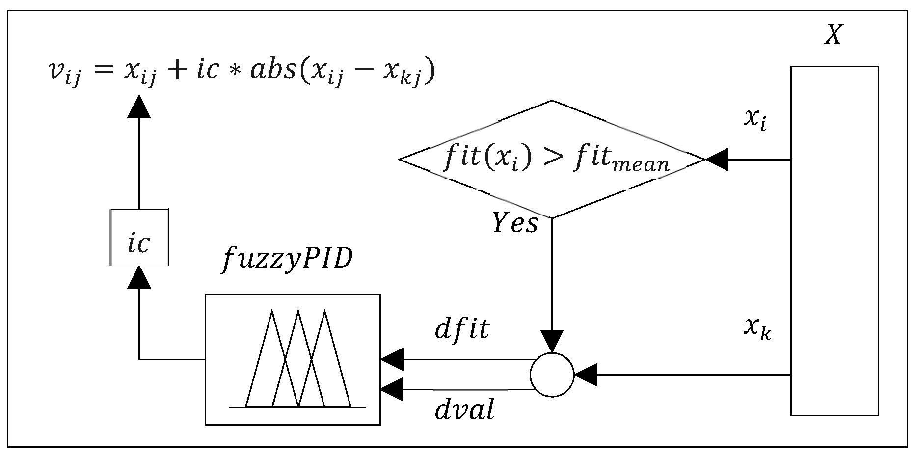
The contribution of aABC to standard ABC is that during the scanning, the algorithm can adaptively regulate the local/global search focus and direct artificial onlooker bees to better solutions. Essentially, standard ABC has the property that it can be propagated throughout the search space without the need for a large population. While the algorithm makes a random search on a global scale with artificial scout bees, artificial employed and artificial onlooker bees make a random search on a local scale. This is because the random coefficient assigned to ϕ in Equation (2) in the range of [–1 1] allows the algorithm to scan larger and smaller search regions.

In the onlooker bee procedure of the improved aABC (iaABC), instead of assigning a random value to the ϕ, an “intelligent coefficient (ic)” is assigned that aims at a better solution. First, the fitness of the existing solutions is normalized by proportioning it to the best fitness achieved so far. Then, with Equation (7), the difference in normalized fitness values (dfit) is calculated.

$$dfit={\displaystyle \frac{fit\left(x_i\right)}{fi{t}_{best}}}-{\displaystyle \frac{fit\left(x_k\right)}{fi{t}_{best}}}$$

(7)

After defining dfit with Equation (8), the values in the selected dimension of the solutions are normalized within the specified bounds, and their differences (dval) are calculated.

$$dval=({\displaystyle \frac{x_{ij}-x_{ij}^{min}}{x_{ij}^{max}-x_{ij}^{min}}})-({\displaystyle \frac{x_{kj}-x_{kj}^{min}}{x_{kj}^{max}-x_{kj}^{min}}})$$

(8)

The calculated dfit and dval are entered as input to the fuzzy PID control system, and the intelligent coefficient (ic) is obtained. The obtained coefficient is used in Equation (9) to produce a new solution.

$$v_{ij}=x_{ij}+ic\ast abs(x_{ij}-x_{kj})$$

(9)

Note that in Equation (9), unlike Equation (2), the absolute value of the difference between solution members is used. The solution-producing process in the onlooker bee procedure of iaABC is illustrated in Figure 1.

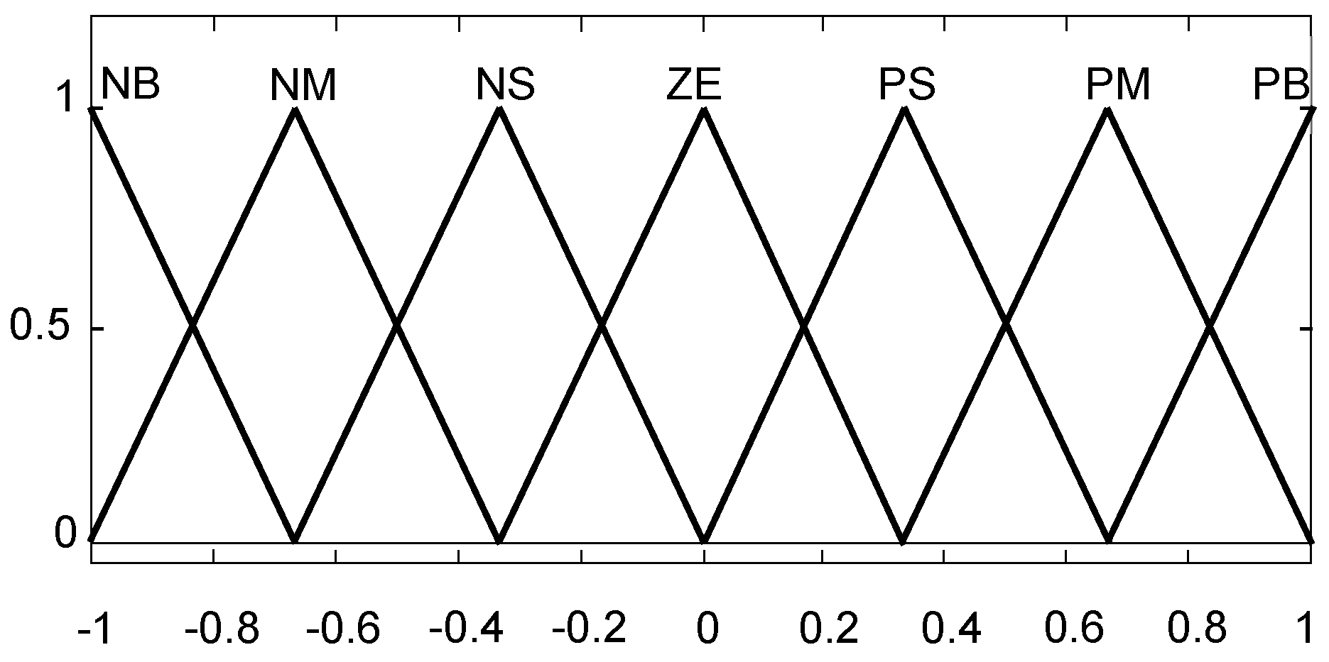
In the fuzzy PID design, fuzzy sets with the same properties for all variables were designed. For the type of fuzzy sets, the triangular membership function (MF) (trimf), whose graphs are given in Figure 2, was selected. The following linguistic labels were used for their names: “Negative Big” (NB), “Negative Medium” (NM), “Negative Small” (NS), “Zero” (ZE), “Positive Small” (PS), “Positive Medium” (PM), and “Positive Big” (PB).

The parameter values assigned for the trimf membership function (MF) are presented in

Table 1. Parameter settings for trimf MFs in fuzzy-PID.

	NB	NM	NS	ZE	PS	PN	PB
a	−1.33	−1	−0.66	−0.33	0	0.33	0.66
b	−1	−0.66	−0.33	0	0.33	0.66	1
c	−0.66	−0.33	0	0.33	0.66	1	1.33

.

In the proposed model, a fuzzy rule-based system is designed. While preparing fuzzy rules, it aims to bring the solutions whose values are far from each other in the selected dimension closer to a better solution and to perform a local search for the solutions whose values and fitness are close to each other in the dimension.

The rule table prepared for fuzzy-PID is presented in

Table 2. The fuzzy rule table for fuzzy-PID.

		dfit
		NL	NM	NS	ZE	PS	PM	PL
dval	NL	PL	PL	PL	PL	PM	ZE	ZE
	NM	PL	PL	PL	PL	PM	ZE	ZE
	NS	PM	PM	PM	PS	ZE	NM	NM
	ZE	PM	PM	PS	ZE	NS	NM	NM
	PS	PM	PM	ZE	NS	NM	NM	NM
	PM	ZE	ZE	NM	NL	NL	NL	NL
	PL	ZE	ZE	NM	NL	NL	NL	NL

.

To calculate the function value of the optimization problem h, assume that the computing time is the complexity, which is O(h). Let the maximum number of iterations determined to solve this problem be the I_max and the colony size CS. In this case, the calculation complexity time for the standard ABC is O[I_max * (CS * h + CS * h)] = O(I_max * CS * h) [38]. In aABC, the total compliance (fit_mean) value of the solutions is calculated and shared according to the compliance value of the solutions. In this case, the complexity of the calculation time for aABC is O[I_max * (CS * h + 2 * CS * h)] = O(I_max * CS * h). In iaABC, dfit and dval values are also calculated. If the calculation time for iaABC is the complexity, it is O[I_max * (CS * h + 4 * CS * h)] = O(I_max * CS * h).

4. Experimental Studies

The proposed method was implemented using MATLAB version 2023b on a PC with an Intel i7-4710MQ processor (Intel Corporation, Santa Clara, CA, USA), operating at 2.50 GHz, with 16 GB RAM and Windows 10 Home Premium (SP1) as the operating system. The performance of iaABC was initially evaluated on single-objective numerical optimization problems for statistical analysis. Subsequently, the method was applied to three-dimensional Wireless Sensor Networks (WSNs). The performance of iaABC for both CEC 2022 and WSNs was compared with ABC optimization algorithms (standard ABC and iABC) and modern algorithms such as the Adaptive Flower Pollination Algorithm (AFPA) [11], Composite Proactive Particles in Swarm Optimization (Co-PPSO) [39], Salp Swarm Algorithm (SSA) [40], and Sine Cosine Algorithm (SCA) [41]. The preferred methods for positioning in 3D WSNs are generally versions of PSO. In this context, we selected the Co-PPSO algorithm for comparison, as it has also successfully produced solutions for the CEC 2022 test suits. The strategy employed in our study is based on the approach outlined in reference [1]. Consequently, we chose the AFPA from the relevant study for comparison. Other methods highlighted in our research are recognized as state-of-the-art algorithms.

4.1. Statistical Testing of iaABC

For statistical analysis, the solution derivation approach, convergence performance, and exploitation/exploration balance of the proposed method were tested using numerical optimization problems (NOPs). Single-objective NOPs were used for testing because these problems form the basis of more complex problems, such as many-objective, niche, and mixed optimization problems. In this context, improvements in single-objective optimization algorithms may also affect other areas. Therefore, to conduct statistical tests on iaABC, test suits that were proposed for a special session and competition on Single Objective Bound Constrained Real Parameter Numerical Optimization, which took place during the Congress on Evolutionary Computation (CEC) 2022 [42], were selected.

4.1.1. CEC 2022 Benchmark Functions

CEC 2022 benchmark functions are based on real parameter optimization to promote symbiosis. Functions are parameterized by including full rotation operators. The main motive behind this parameterization is to test the effect of all algorithms on full rotation benchmark functions. For this goal, 12 scalable benchmark problems with 10-D and 20-D are proposed. All test functions are shifted to o and are scalable, defined minimization problems.

The CEC 2022 test functions are categorized into four distinct classifications. The names of the functions, their corresponding categories, and the optimal values are presented in

Table 3. CEC 2022 benchmark functions.

Category	No	Name	Best
Unimodal	F1	Shifted and full Rotated Zakharov Function	300
Basic	F2	Shifted and full Rotated Rosenbrock’s Function	400
	F3	Shifted and full Rotated Expanded Schaffer’s f6 Function	600
	F4	Shifted and full Rotated Non-Continuous Rastrigin’s Function	800
	F5	Shifted and full Rotated Levy Function	900
Hybrid	F6	Hybrid Function 1 (N = 3)	1800
	F7	Hybrid Function 2 (N = 6)	2000
	F8	Hybrid Function 3 (N = 5)	2200
Composition	F9	Composition Function 1 (N = 5)	2300
	F0	Composition Function 2 (N = 4)	2400
	F11	Composition Function 3 (N = 5)	2600
	F12	Composition Function 4 (N = 6)	2700

. F1 is indicative of unimodal functions, whereas functions F2 through F5 are classified as basic functions. Functions F6 through F8 are designated as hybrid functions, and functions F9 through F12 are categorized as composition functions. The search domain is bounded by [−100, 100]^D. Functions F1 through F5 are derived from a fundamental function via shifting and rotation. In functions F6 to F8, the variables are arbitrarily split into specific subcomponents and different basic functions are applied to them. Each hybrid function has a different number of basic functions.

The F9 and F10 functions successfully combine the properties of the functions within them while maintaining consistency in global and local optima, while the composition functions use shifted and rotated forms of the underlying functions. This methodology enhances the complexity of the functions and imposes additional challenges on the algorithm’s performance [42].

4.1.2. Parameter Settings for CEC 2022 Benchmark Functions

In this study, the statistical testing of iaABC was carried out according to the rules outlined in CEC 2022. The values assigned to the control parameters of the competing algorithms were determined following the guidelines in [42]. As initial solutions, the seeds of the Mersenne Twister pseudo-random generator provided by the competition organizers were used. The algorithms were run 30 times independently for each test suite and the results were saved. Once the experiments were completed, the results such as the most successful, worst, median, average, and SD obtained for each pattern were also presented in a table.

The termination criterion for evaluating the objective function (MaxFEs) for each study was set to a maximum of 200,000 for 10-D and a maximum of 1,000,000 for 20-D.

4.1.3. iaABC’s Performance on CEC 2022 Benchmark Functions

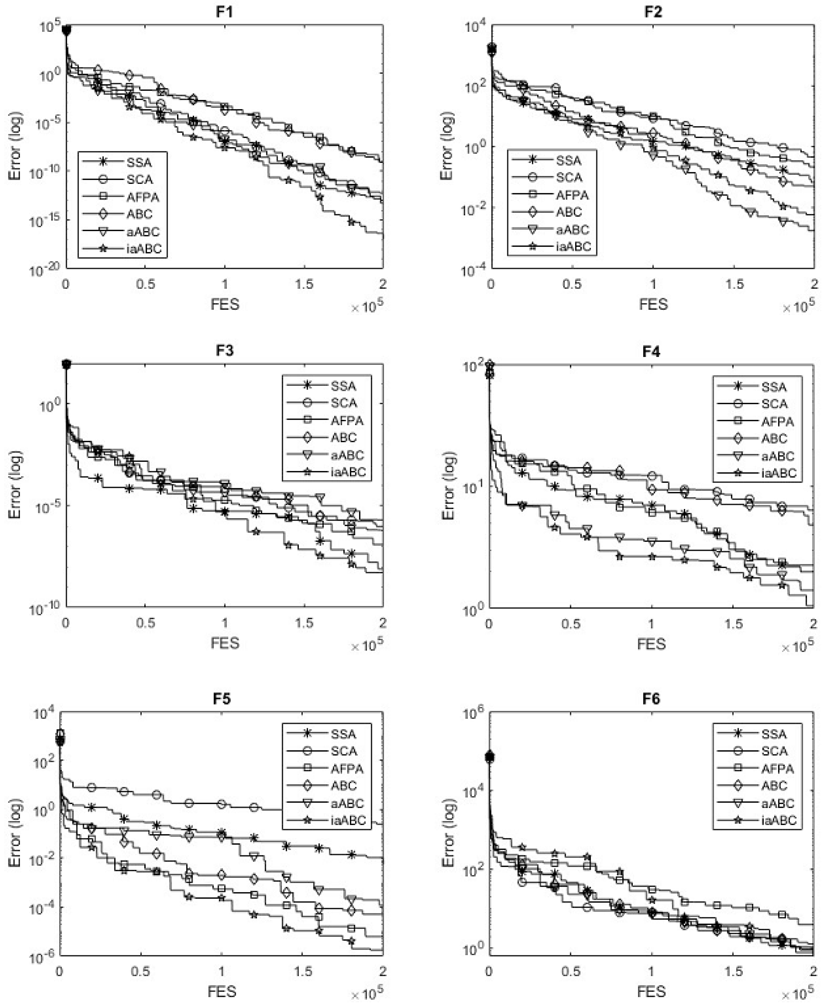
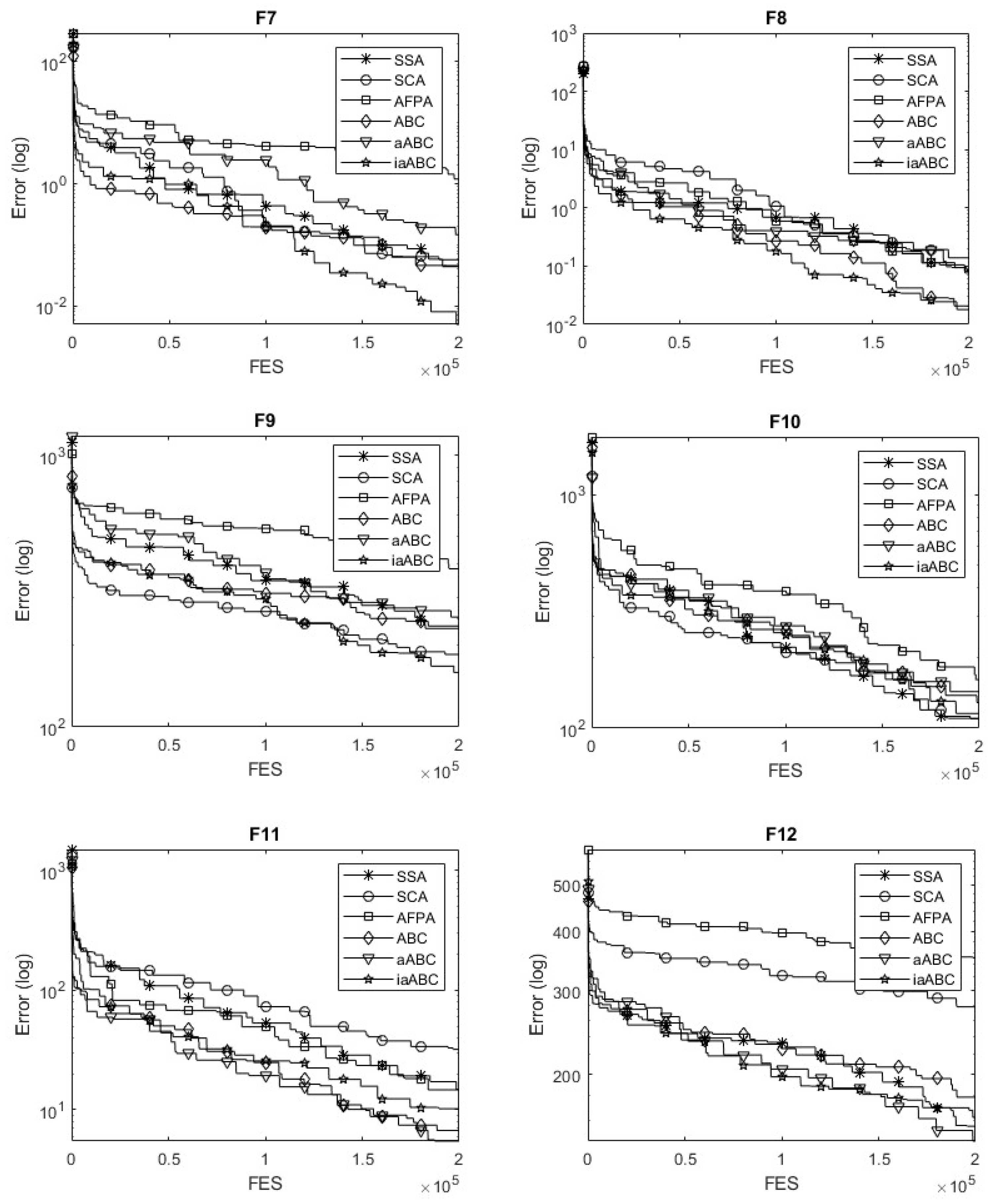
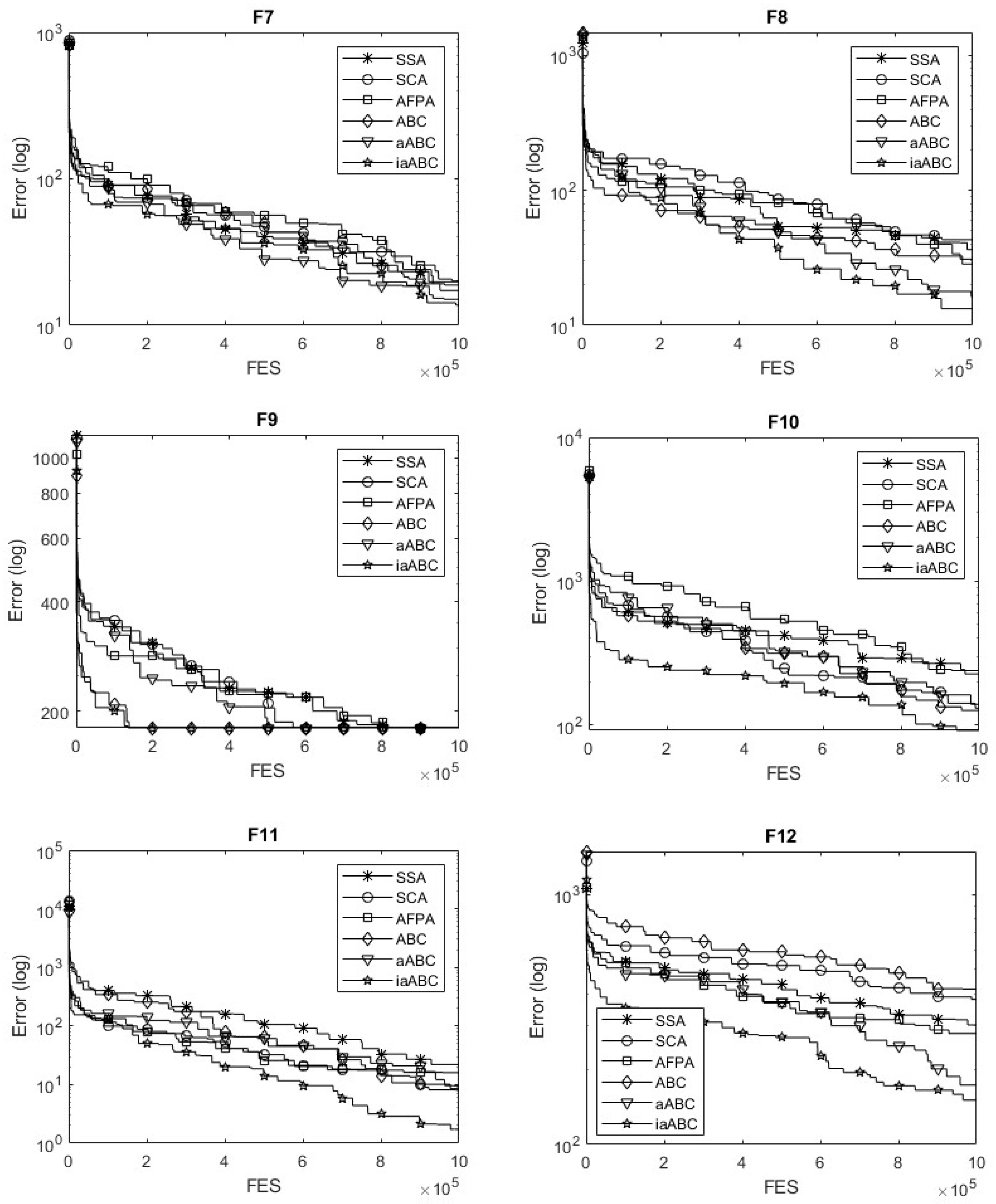
The statistical performance of iaABC on CEC 2022 benchmark functions is analyzed based on error. The error is the difference between the global optimum value for the function and the best value produced by the algorithm. The results of the errors of the 10-dimensional experiments with the algorithms are given in

Table 4. Results of competitive algorithms for CEC 2022 benchmarks (D = 10).

No	Method	Best	Worst	Median	Mean	SD	No	Method	Best	Worst	Median	Mean	SD
F1	Co-PPSO	0.00E+00	0.00E+00	0.00E+00	0.00E+00	0.00E+00	F7	Co-PPSO	2.04E-08	2.20E+01	1.80E+00	8.84E+00	9.81E+00
	SSA	0.00E+00	2.41E+00	0.00E+00	0.65E+00	7.01E-07		SSA	5.32E-01	2.43E+01	1.29E+01	1.35E+01	7.10E+00
	SCA	0.00E+00	3.09E+00	0.00E+00	0.77E+00	5.64E-06		SCA	2.43E-01	2.45E+01	1.32E+01	1.05E+01	7.59E+00
	AFPA	0.00E+00	0.00E+00	0.00E+00	0.00E+00	0.00E+00		AFPA	1.45E+00	2.41E+01	1.25E+01	1.35E+01	6.02E+00
	ABC	0.00E+00	0.00E+00	0.00E+00	0.00E+00	0.00E+00		ABC	1.91E-01	2.73E+01	1.09E+01	1.22E+01	7.54E+00
	aABC	0.00E+00	0.00E+00	0.00E+00	0.00E+00	0.00E+00		aABC	5.97E-02	2.72E+01	1.10E+01	1.26E+01	8.54E+00
	iaABC	0.00E+00	0.00E+00	0.00E+00	0.00E+00	0.00E+00		iaABC	0.00E+00	2.13E+01	9.64E+00	1.10E+01	6.35E+00
F2	Co-PPSO	5.57E-06	9.04E+00	1.71E-03	1.70E+00	2.42E+00	F8	Co-PPSO	1.02E-01	2.24E+01	2.06E+01	1.54E+01	9.20E+00
	SSA	1.89E+00	4.82E+01	2.18E+01	2.48E+01	1.61E+01		SSA	9.70E-01	3.85E+01	1.79E+01	1.83E+01	1.17E+01
	SCA	2.70E-02	7.73E+00	2.62E+00	2.50E+00	1.42E+00		SCA	4.44E-01	3.81E+01	1.97E+01	2.01E+01	1.33E+01
	AFPA	6.14E-01	3.43E+01	1.46E+01	1.56E+01	9.58E+00		AFPA	8.65E-01	3.84E+01	1.07E+01	1.54E+01	1.22E+01
	ABC	4.86E-02	4.62E+01	2.50E+00	2.23E+00	1.31E+00		ABC	2.70E+00	3.98E+01	2.41E+01	2.44E+01	1.13E+01
	aABC	4.99E-02	1.42E+01	6.22E+00	5.98E+00	4.37E+00		aABC	1.01E+00	3.94E+01	1.48E+01	1.88E+01	1.36E+01
	iaABC	6.20E-03	2.90E+00	1.37E+00	1.48E+00	9.27E-01		iaABC	1.96E-01	2.56E+01	1.48E+01	1.38E+01	7.51E+00
F3	Co-PPSO	0.00E+00	0.00E+00	0.00E+00	0.00E+00	0.00E+00	F9	Co-PPSO	2.30E+02	2.30E+02	2.30E+02	2.30E+02	8.70E-02
	SSA	3.37E-03	9.68E-01	3.88E-01	4.51E-01	3.17E-01		SSA	2.31E+02	2.49E+02	2.39E+02	2.40E+02	5.66E+00
	SCA	0.00E+00	0.00E+00	0.00E+00	0.00E+00	0.00E+00		SCA	2.30E+02	2.49E+02	2.35E+02	2.38E+02	6.69E+00
	AFPA	1.29E-04	4.86E-02	2.18E-02	2.41E-02	1.49E-02		AFPA	2.30E+02	2.50E+02	2.40E+02	2.40E+02	6.23E+00
	ABC	0.00E+00	0.00E+00	0.00E+00	0.00E+00	0.00E+00		ABC	2.30E+02	2.30E+02	2.30E+02	2.30E+02	1.26E-01
	aABC	0.00E+00	0.00E+00	0.00E+00	0.00E+00	0.00E+00		aABC	2.30E+02	2.30E+02	2.30E+02	2.30E+02	1.24E-01
	iaABC	0.00E+00	0.00E+00	0.00E+00	0.00E+00	0.00E+00		iaABC	2.30E+02	2.30E+02	2.30E+02	2.30E+02	1.01E-01
F4	Co-PPSO	1.99E+00	1.39E+00	6.96E+00	6.70E+00	2.60E+00	F10	Co-PPSO	1.00E+02	1.00E+02	1.00E+02	1.00E+02	6.54E-02
	SSA	2.76E+00	1.08E+01	7.48E+00	7.33E+00	2.46E+00		SSA	1.10E+02	2.86E+02	1.90E+02	1.88E+02	5.25E+01
	SCA	3.43E+00	1.05E+01	7.59E+00	7.17E+00	1.99E+00		SCA	1.03E+02	2.80E+02	1.88E+02	1.90E+02	6.16E+01
	AFPA	2.40E+00	1.05E+01	5.73E+00	5.97E+00	2.78E+00		AFPA	1.05E+02	2.97E+02	2.31E+02	2.15E+02	6.51E+00
	ABC	2.12E+00	1.08E+01	6.90E+00	6.66E+00	2.76E+00		ABC	1.00E+02	1.10E+02	1.06E+02	1.06E+02	3.03E+00
	aABC	2.01E+00	1.05E+01	6.84E+00	6.62E+00	2.76E+00		aABC	1.00E+02	1.10E+02	1.06E+02	1.05E+02	2.81E+00
	iaABC	2.02E+00	1.10E+01	6.06E+00	6.31E+00	2.61E+00		iaABC	1.00E+02	1.00E+02	1.00E+02	1.00E+02	0.00E+00
F5	Co-PPSO	0.00E+00	0.00E+00	0.00E+00	0.00E+00	0.00E+00	F11	Co-PPSO	0.00E+00	3.00E+02	0.00E+00	2.50E+01	7.96E+01
	SSA	0.00E+00	0.00E+00	0.00E+00	0.00E+00	0.00E+00		SSA	6.56E+00	3.86E+02	2.23E+02	2.12E+02	1.18E+02
	SCA	8.32E-02	4.97E-01	2.45E-01	2.78E-01	1.27E-01		SCA	3.10E+00	3.99E+02	2.14E+02	2.20E+02	1.06E+02
	AFPA	9.68E-03	4.95E-01	2.50E-01	2.52E-01	1.52E-01		AFPA	6.38E-01	3.93E+02	2.43E+02	2.20E+02	1.23E+02
	ABC	0.00E+00	0.00E+00	0.00E+00	0.00E+00	0.00E+00		ABC	2.37E+00	2.94E+02	1.31E+02	1.42E+02	8.85E+01
	aABC	1.33E-02	4.98E-01	2.38E-01	2.46E-01	1.52E-01		aABC	8.74E-01	2.85E+02	1.29E+02	1.41E+02	7.23E+01
	iaABC	0.00E+00	0.00E+00	0.00E+00	0.00E+00	0.00E+00		iaABC	0.00E+00	4.64E+01	2.02E+01	2.37E+01	1.24E+01
F6	Co-PPSO	7.00E+00	1.76E+03	1.11E+02	3.33E+02	4.30E+02	F12	Co-PPSO	1.63E+02	1.65E+02	1.65E+02	1.65E+02	4.41E-01
	SSA	5.87E+01	1.73E+03	7.89E+02	8.65E+02	5.00E+02		SSA	1.63E+02	2.00E+02	1.79E+02	1.80E+02	1.07E+01
	SCA	9.32E+00	1.76E+03	6.80E+00	7.52E+02	4.33E+02		SCA	1.66E+02	1.80E+02	1.71E+02	1.73E+02	4.04E+00
	AFPA	9.76E+01	1.99E+03	1.14E+03	1.04E+03	5.98E+02		AFPA	1.65E+02	1.79E+02	1.73E+02	1.73E+02	3.77E+00
	ABC	5.35E+01	1.62E+03	7.62E+02	7.65E+02	5.10E+02		ABC	1.62E+02	1.65E+02	1.63E+02	1.64E+02	8.98E-01
	aABC	1.58E+01	1.97E+03	1.14E+03	1.06E+03	6.80E+02		aABC	1.62E+02	1.65E+02	1.63E+02	1.64E+02	8.87E-01
	iaABC	1.41E+01	1.93E+03	1.13E+03	1.03E+03	6.31E+02		iaABC	1.62E+02	1.65E+02	1.63E+02	1.63E+02	7.72E-01

, while the convergence error lines are given in Figure 3. The results regarding the errors and the convergence error lines obtained for the 20-dimensional experiments are presented in

Table 5. Results of competitive algorithms for CEC 2022 benchmarks (D = 20).

No	Method	Best	Worst	Median	Mean	SD	No	Method	Best	Worst	Median	Mean	SD
F1	Co-PPSO	0.00E+00	0.00E+00	0.00E+00	0.00E+00	0.00E+00	F7	Co-PPSO	2.03E+01	4.88E+01	2.67E+01	2.96E+01	7.31E+00
	SSA	9.54E-02	9.98E-01	4.94E-01	4.92E-01	2.67E-01		SSA	2.16E+01	4.80E+01	3.63E+01	3.73E+01	6.84E+00
	SCA	4.98E-03	1.00E+00	6.38E-01	5.48E-01	3.24E-01		SCA	2.25E+01	4.46E+01	3.57E+01	3.43E+01	6.57E+00
	AFPA	0.00E+00	1.19E-02	4.46E-01	4.84E-01	2.86E-01		AFPA	2.27E+01	4.79E+01	3.59E+01	3.60E+01	6.95E+00
	ABC	0.00E+00	0.00E+00	0.00E+00	0.00E+00	0.00E+00		ABC	2.01E+01	4.68E+01	2.87E+01	3.02E+01	7.96E+00
	aABC	0.00E+00	0.00E+00	0.00E+00	0.00E+00	0.00E+00		aABC	1.98E+01	4.58E+01	3.36E+01	3.31E+01	8.49E+00
	iaABC	0.00E+00	0.00E+00	0.00E+00	0.00E+00	0.00E+00		iaABC	1.81E+01	4.67E+01	3.50E+01	3.49E+01	8.72E+00
F2	Co-PPSO	1.40E+01	1.94E+01	1.65E+01	1.66E+01	1.16E+00	F8	Co-PPSO	2.04E+01	2.64E+01	2.14E+01	2.18E+01	1.29E+00
	SSA	1.52E+01	3.50E+01	2.31E+01	2.40E+01	6.47E+00		SSA	2.05E+01	3.10E+01	2.42E+01	2.50E+01	3.14E+00
	SCA	1.66E+01	3.35E+01	2.37E+01	2.42E+01	5.41E+00		SCA	1.90E+01	3.05E+01	2.49E+01	2.49E+01	3.70E+00
	AFPA	1.59E+01	3.49E+01	2.33E+01	2.33E+01	5.10E+00		AFPA	1.91E+01	3.00E+01	2.60E+01	2.51E+01	3.46E+00
	ABC	1.09E+01	2.17E+01	1.67E+01	1.67E+01	3.46E+00		ABC	1.86E+01	2.49E+01	2.24E+01	2.19E+01	1.87E+00
	aABC	1.01E+01	2.19E+01	1.54E+01	1.56E+01	3.70E+00		aABC	1.83E+01	2.44E+01	2.23E+01	2.19E+01	1.65E+00
	iaABC	1.01E+01	2.05E+01	1.39E+01	1.49E+01	3.05E+00		iaABC	1.80E+01	2.50E+01	2.10E+01	2.11E+01	2.13E+00
F3	Co-PPSO	0.00E+00	1.48E-03	2.54E-06	6.48E-05	2.71E-04	F9	Co-PPSO	1.80E+02	1.82E+02	1.80E+02	1.80E+02	3.76E-01
	SSA	7.01E-03	9.97E-03	8.79E-03	8.63E-03	8.51E-04		SSA	1.80E+02	1.85E+02	1.83E+02	1.83E+02	1.37E+00
	SCA	7.51E-03	2.21E-02	1.50E-02	1.51E-02	4.92E-03		SCA	1.80E+02	1.85E+02	1.83E+02	1.83E+02	1.56E+00
	AFPA	8.25E-03	2.14E-02	1.32E-02	1.40E-02	4.26E-03		AFPA	1.80E+02	1.84E+02	1.82E+02	1.82E+02	1.25E+00
	ABC	1.15E-06	9.62E-05	6.09E-05	5.55E-05	2.92E-05		ABC	1.80E+02	1.80E+02	1.80E+02	1.80E+02	1.77E-02
	aABC	1.23E-07	9.92E-06	4.30E-06	4.84E-06	3.16E-06		aABC	1.80E+02	1.80E+02	1.80E+02	1.80E+02	1.46E-02
	iaABC	0.00E+00	9.93E-06	6.04E-06	5.85E-05	2.69E-06		iaABC	1.80E+02	1.80E+02	1.80E+02	1.80E+02	1.41E-02
F4	Co-PPSO	5.97E+00	3.38E+01	1.74E+01	1.92E+01	6.02E+00	F10	Co-PPSO	1.00E+02	4.89E+02	1.00E+02	1.17E+02	7.37E+01
	SSA	8.10E+00	5.17E+01	3.25E+01	3.30E+01	1.42E+01		SSA	1.46E+02	4.94E+02	3.03E+02	3.10E+02	1.03E+02
	SCA	8.52E+00	5.10E+01	2.96E+01	2.91E+01	1.48E+01		SCA	1.54E+02	4.85E+02	3.15E+02	3.18E+02	9.58E+01
	AFPA	1.30E+01	5.18E+01	3.59E+01	3.37E+01	1.27E+01		AFPA	1.31E+02	4.69E+02	3.37E+02	3.13E+02	1.11E+02
	ABC	5.12E+00	3.98E+01	1.60E+01	1.88E+01	1.12E+01		ABC	1.12E+02	3.77E+02	2.42E+02	2.40E+02	7.60E+01
	aABC	3.99E+00	3.81E+01	2.07E+01	2.21E+01	9.59E+00		aABC	1.03E+02	3.72E+02	2.59E+02	2.59E+02	7.94E+01
	iaABC	3.24E+00	3.90E+01	2.34E+01	2.42E+01	1.10E+01		iaABC	9.73E+01	3.74E+02	2.49E+02	2.35E+02	8.09E+01
F5	Co-PPSO	0.00E+00	4.00E+00	8.95E-02	5.36E-01	9.21E-01	F11	Co-PPSO	0.00E+00	4.00E+02	3.00E+02	3.13E+02	9.73E+01
	SSA	1.05E-01	4.90E+00	2.55E+00	2.40E+00	1.47E+00		SSA	6.50E+01	9.94E+02	5.78E+02	5.36E+02	3.14E+02
	SCA	1.29E-01	4.84E+00	2.40E+00	2.46E+00	1.35E+00		SCA	3.54E+01	9.97E+02	5.00E+02	4.89E+02	2.70E+02
	AFPA	6.45E-02	4.45E+00	2.09E+00	2.37E+00	1.39E+00		AFPA	2.13E+01	9.50E+02	5.58E+02	5.30E+02	2.68E+02
	ABC	2.40E-04	3.86E+00	1.83E+00	1.83E+00	1.24E+00		ABC	3.74E+00	6.00E+02	3.06E+02	3.13E+02	1.99E+02
	aABC	2.54E-01	3.80E+00	1.70E+00	1.89E+00	9.66E-01		aABC	6.02E+00	5.55E+02	2.62E+02	2.80E+02	1.73E+02
	iaABC	0.00E+00	3.58E+00	1.64E+00	1.83E+00	1.09E+00		iaABC	2.76E+00	5.83E+02	2.79E+02	2.99E+02	1.95E+02
F6	Co-PPSO	4.41E+01	2.18E+04	3.91E+03	5.59E+03	5.62E+03	F12	Co-PPSO	1.95E+02	1.99E+02	1.96E+02	1.96E+02	1.00E+00
	SSA	1.45E+02	5.37E+03	2.83E+03	2.90E+03	1.50E+03		SSA	2.05E+02	3.48E+02	2.93E+02	2.81E+02	4.82E+01
	SCA	5.31E+02	2.92E+04	1.45E+04	1.48E+04	9.28E+03		SCA	2.51E+02	3.19E+02	2.78E+02	2.84E+02	2.11E+01
	AFPA	3.81E+02	2.35E+04	1.37E+04	1.29E+04	6.87E+03		AFPA	2.80E+02	3.05E+02	2.90E+02	2.91E+02	7.63E+00
	ABC	1.17E+02	2.68E+04	1.73E+04	1.55E+04	8.45E+03		ABC	2.09E+02	3.49E+02	2.73E+02	2.78E+02	4.36E+01
	aABC	2.82E+01	2.41E+04	1.28E+04	1.23E+04	7.33E+03		aABC	1.72E+02	2.64E+02	2.16E+02	2.15E+02	2.73E+01
	iaABC	4.29E+01	2.41E+04	1.12E+04	1.22E+04	7.53E+03		iaABC	1.55E+02	1.91E+02	1.74E+02	1.73E+02	1.06E+01

and Figure 4, respectively. When the error is 1E-8 or less, it is evaluated as 0. The results obtained with Co-PPSO are taken from [39].

According to the statistical results for the 10-D case presented in Table 4, the iaABC algorithm achieved more successful outcomes than other algorithms in 8 out of 12 test functions. Examining the convergence error graphs for the algorithms, shown in Figure 3, indicates that the proposed method demonstrates effective convergence performance. For the unimodal function, iaABC, like many other algorithms, produced the best solution in all trials. In this context, the proposed method has excellent performance and good robustness. iaABC produces successful solutions for the basic functions used for comparison, and the error curves in Figure 3 prove that iaABC has a more efficient convergence performance than other algorithms. The Rosenbrock function is not convex and contains many narrow hillocks. Because the hillocks are very sharp, metaheuristic methods cannot identify points that can be advanced in the problem [43].

However, iaABC produces solutions with the most successful mean and SD values for F2 and reaches a convergence accuracy of 1E-3. However, it also produces the optimal result for the F3 and F5 functions. Regarding the compared hybrid functions, iaABC produced the optimal result for the F7 function and achieved 1E-1 convergence accuracy for the F8 function. Composition functions are formed by combining various complex functions, each of which may have multiple local optima. This complexity presents a challenge for the optimization capabilities of metaheuristic algorithms. The proposed method successfully identifies the optimal result for the F11 function, which is one of the composition functions. However, it does not achieve optimal results for the F9, F10, or F12 functions. However, when looking at each function from the perspective of 30 trials, the convergence accuracy of iaABC reached 1E+2. When these results are evaluated, it can be said that iaABC has a certain ability for global exploration.

Table 5 displays the results achieved by the algorithms for the 20-dimensional case. Expanding the solution vector poses a challenge for these algorithms. However, the global optimum solution obtained by iaABC matches the target value for the unimodal function F1. When the mean and standard deviation data calculated for 30 trials are examined, it is proven that the algorithm has good robustness. The solution spaces of the basic functions have wavy surfaces. Especially in the Rosenbrock function, the curves are very sharp. iaABC also produced the optimal solution for the F3 and F5 basic functions. However, the results show that the algorithm does not have satisfactory stability.

The convergence data in Figure 4 suggest that the algorithm struggles to optimize many parameters and is trapped in a local optimum. iaABC could not produce optimal solutions for hybrid functions and composition functions. Since composition functions are composed of functions with different characteristics, their search spaces have very complex waves with high and low frequencies. However, the algorithm has a convergence performance close to 10-D solutions for 20-D solutions.

Examining the results shown in Table 4 and Table 5, along with the convergence error curves illustrated in Figure 3 and Figure 4, it can be concluded that the iaABC method has a more effective search strategy and faster convergence speed compared to both the standard ABC and aABC methods.

4.2. Loction Determination in 3D by iaABC

In this study, to determine the optimal locations of target nodes in a 3D environment, the approach using a single anchor node with projections in hexagonal directions, described in detail in [11], was applied.

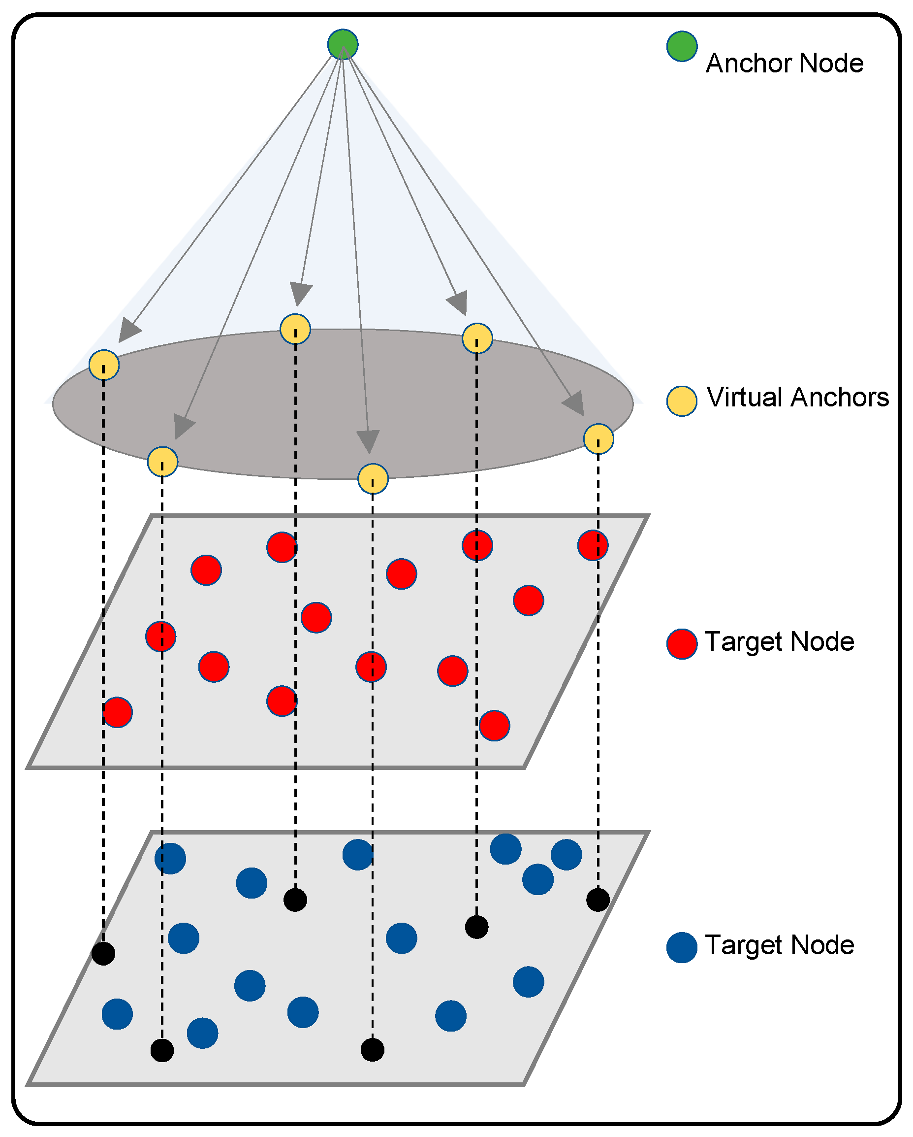
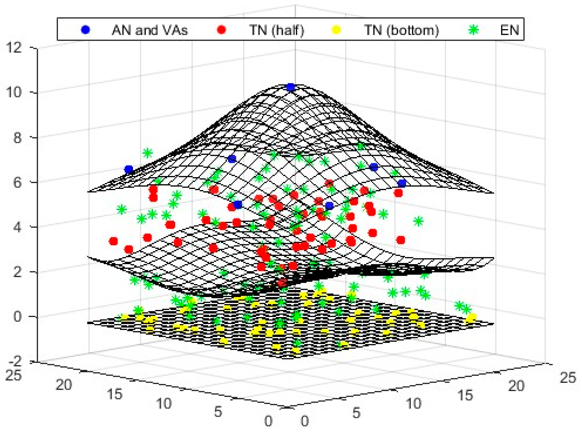
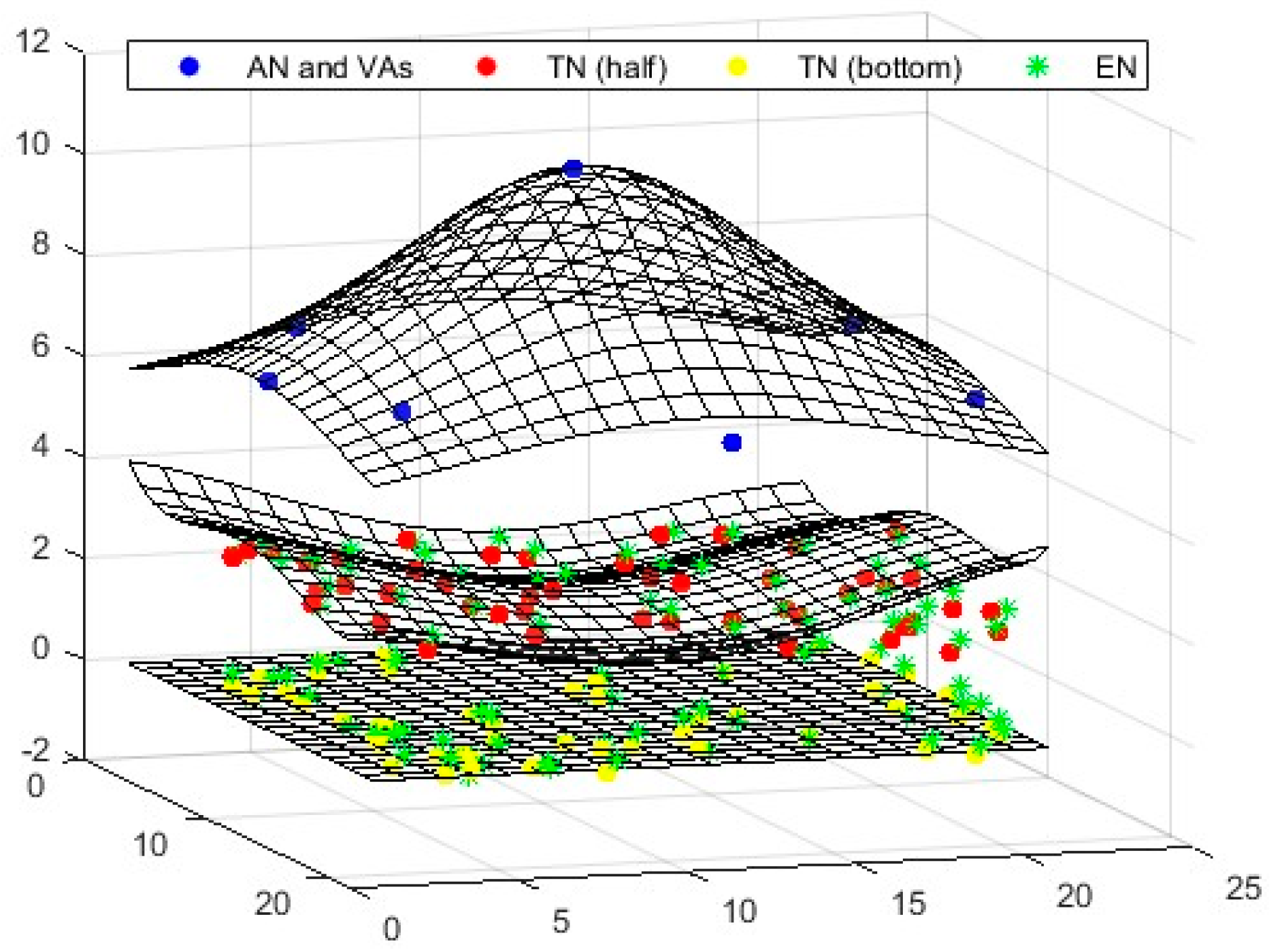
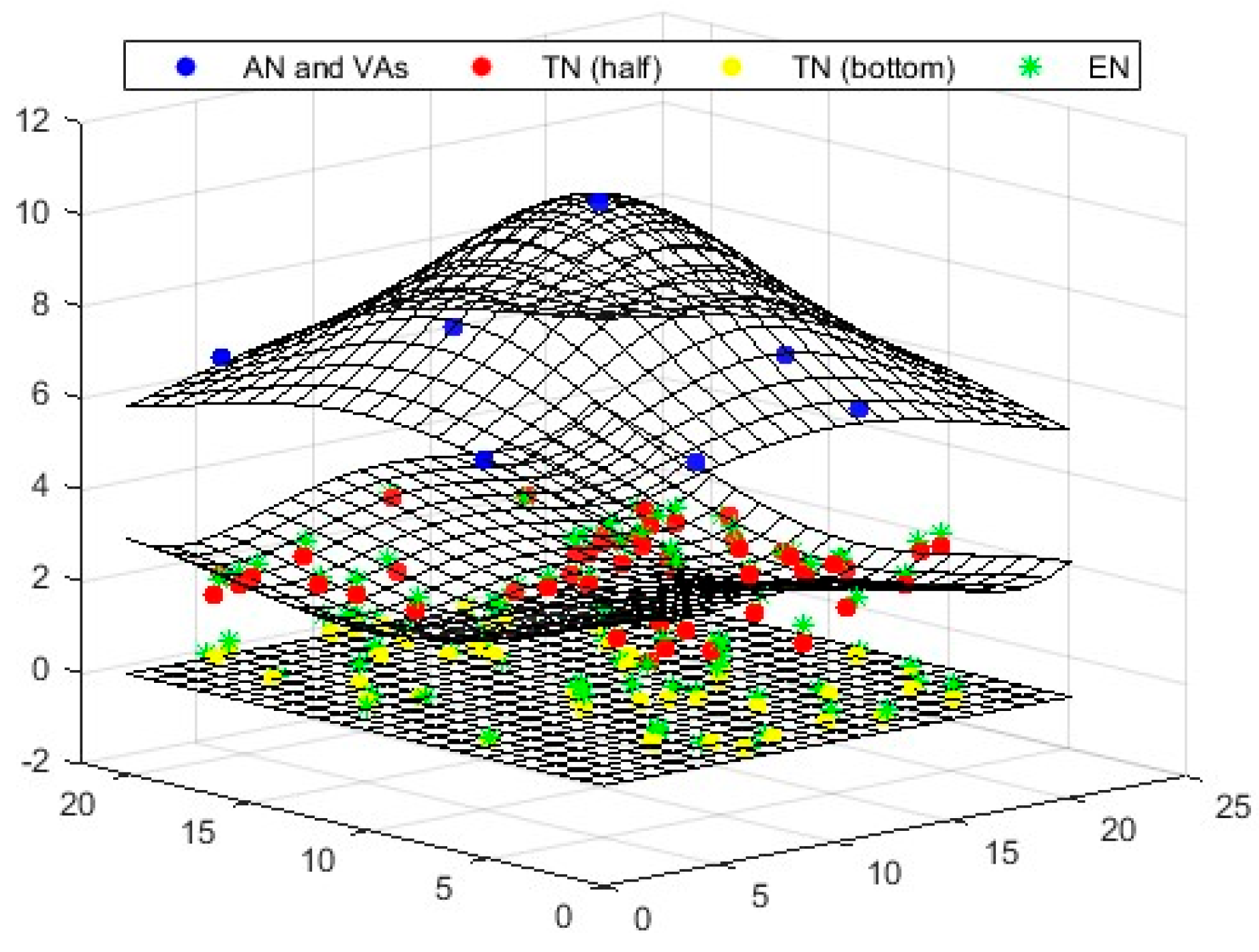
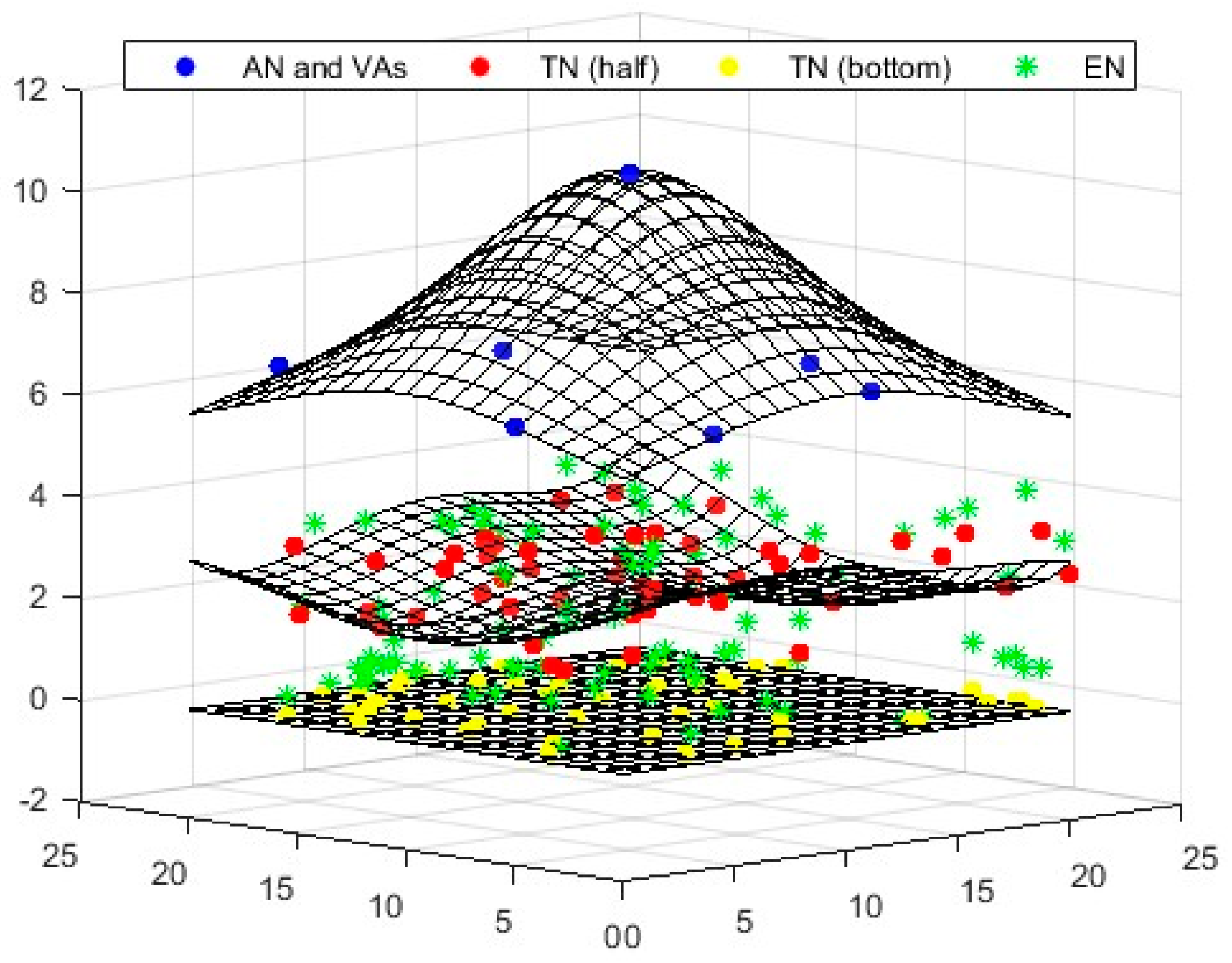
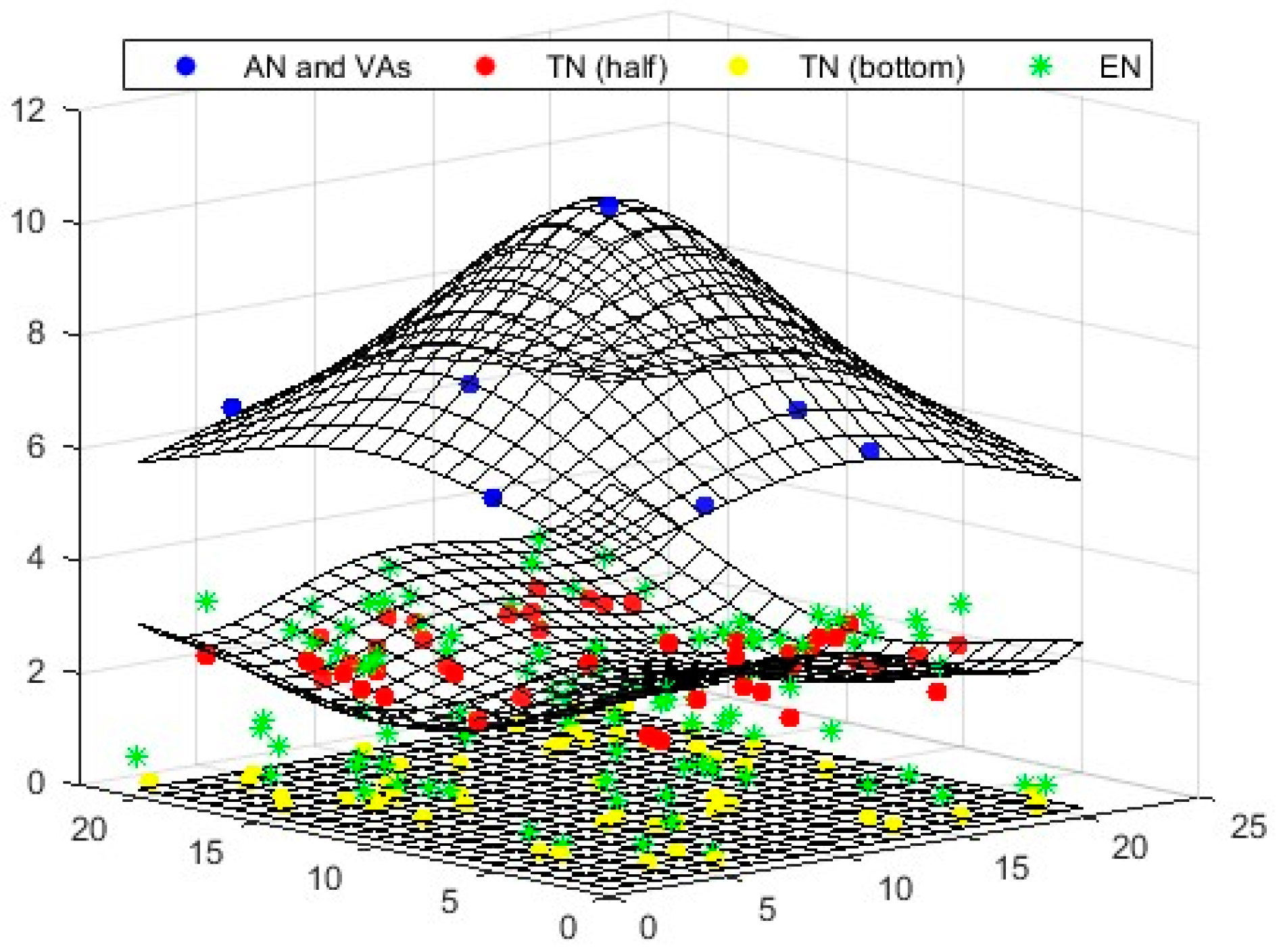
4.2.1. Scenario

To determine the locations of target nodes (TNs), a single anchor node (AN) positioned at the top can be utilized. This method organizes all nodes in three distinct layers: a single AN in the top layer, and 50 randomly distributed TNs in the middle and bottom layers (total 100). Virtual anchors (VAs) are situated in the upper layer, while the TNs are randomly positioned in the lower layers. The beacon signal generated by the AN plays a crucial role in the random placement of the TNs. When a TN falls within the AN’s range, it obtains the Received Signal Strength Indicator (RSSI) information from the anchor, which allows it to calculate the distance between the AN and the TN using the Euclidean formula. In this study, the degree of irregularity (DOI) value was set to 0.01.

After determining this distance, the umbrella projection approach is employed for positioning the TNs, as illustrated in Figure 5. In this approach, six VAs are projected in a circular formation, each spaced 60 degrees apart.

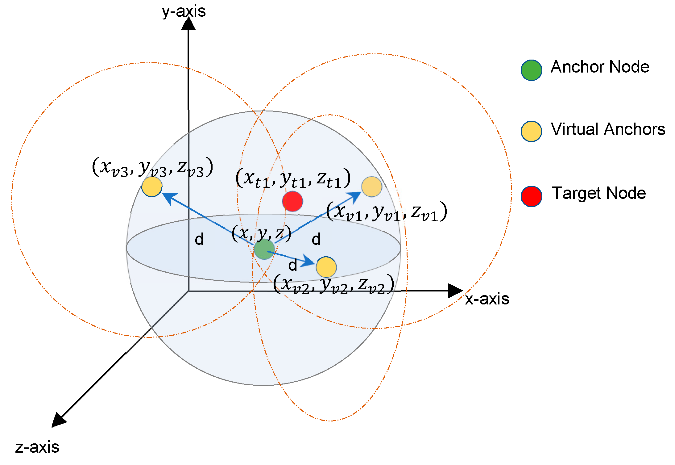
In a 3D environment, as illustrated in Figure 6, four anchors are needed to position the TNs: one anchor to identify the center point and three virtual anchors (VAs). Using the information from the calculated center point, the iaABC method is then applied for optimal positioning.

4.2.2. Mathematical Formulas

The distance (${\widehat{d}}_i$) of any target node to the anchor is calculated by the radio irregularity approach (${\widehat{d}}_i=d_i-D_p+F$). This approach based on the RSSI considers the loss of path (Dp) and fading (F). Also, d_i is calculated with Equation (10).

$$d_i=\sqrt{{\left(x-x_t\right)}^2+{\left(y-y_t\right)}^2+{\left(z-z_t\right)}^2}$$

(10)

where (x_t, y_t, z_t) indicates the target node’s location and (x, y, z) indicates the current location of the anchor node.

The position of the centroid is calculated using Equation (11), which incorporates an AN and the corresponding VNs.

$$\left(x_c,y_c,z_c\right)={\displaystyle \frac{x+{{\displaystyle \sum }}_{i=1}^{3 }{x}_{vi}}{4}},{\displaystyle \frac{y+{{\displaystyle \sum }}_{i=1}^3{y}_{vi}}{4}},{\displaystyle \frac{z+{{\displaystyle \sum }}_{i=1}^3{z}_{vi}}{4}}$$

(11)

where (x_c, y_c, z_c) indicates the coordinates of the center point, while (x_v1, y_v1, z_v1), (x_v2, y_v2, z_v2), and (x_v3, y_v3, z_v3) represent the VN coordinates.

After calculating the centroid, random particles are distributed. The iaABC method is employed to estimate the coordinates of all moving TNs. The estimated coordinates (x_p, y_p, z_p) are saved.

$$f(x_e,y_e,z_e)={\displaystyle \frac{1}{M}}\sum {(\sqrt{{\left(x_p-x_i\right)}^2+{\left(y_p-y_i\right)}^2+{\left(z_p-z_i\right)}^2}-{\widehat{d}}_i)}^2$$

(12)

The fitness value of the solutions is calculated using the mean square error method in Equation (12), which compares the actual coordinates of the TNs with the estimated coordinates.

$$E={\displaystyle \frac{1}{TNs}}\sum \sqrt{{\left(x_t-x_p\right)}^2+{\left(y_t-y_p\right)}^2+{\left(z_t-z_p\right)}^2}$$

(13)

The localization error of the algorithm is calculated using Equation (13). In this context, the objective is min(E).

4.2.3. Parameter Settings for Node Positioning

For a fair comparison, the parameter set provided in

Table 6. Parameter set for the algorithms for optimal location of target nodes.

Algorithm	CS	D	Others
Co-PPSO	30	5
SSA	30	5	c1, c2, c3: 1.494
SCA	30	5	r1, r2, r3, r4: random
AFPA	30	5	pt: Dynamic and adaptive
ABC	30	5	Limit: 75
aABC	30	5	Limit: 75
iaABC	30	5	Limit: 75

was utilized for the competitive algorithms.

Each algorithm was executed 30 times using the parameter values from Table 6, with the MaxFEs set to 20,000. The result and computational time obtained by the competing algorithms for each experiment were saved.

5. Results and Discussion

This section discusses the localization performance of iaABC for WSNs in a 3D environment. In this context, the proposed method is compared with the competitive algorithms used in the previous subsection. The localization results of the competitive algorithms are shown in figures, and the errors in localization and processing times are presented in tables.

In the scenario where all the anchors are kept fixed, the anchors are deployed in a narrower area. By considering all the anchors in the environment, it is possible to find the TNs. However, the convergence performance of the algorithms is low.

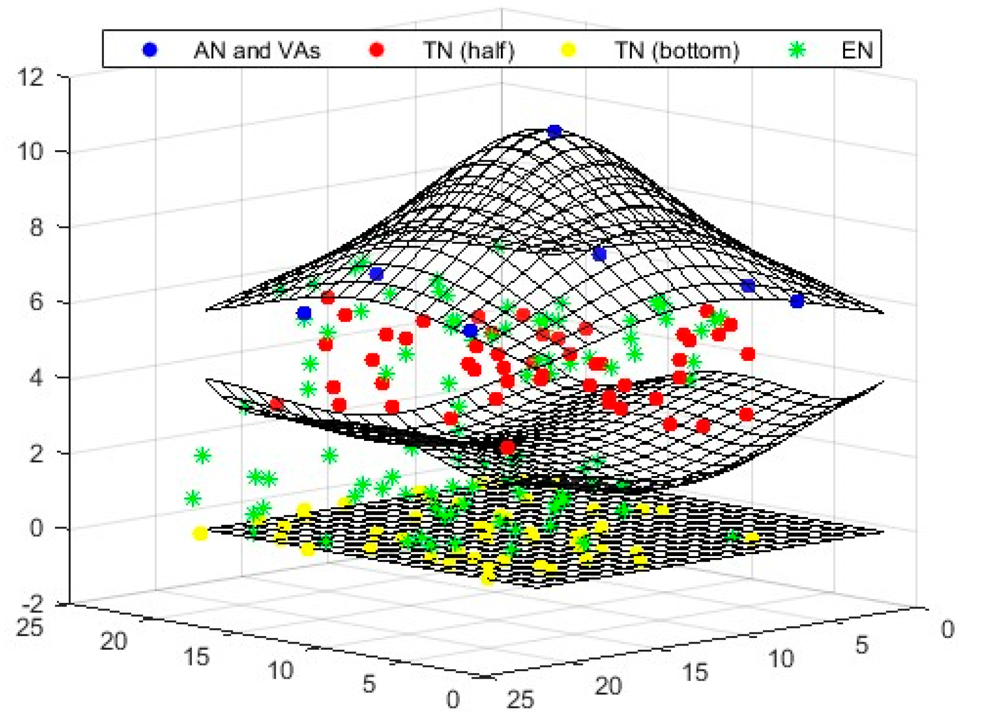
In the mobility-based scenario, the anchor node remains fixed while the target node is mobile. Figure 7, Figure 8, Figure 9, Figure 10, Figure 11, Figure 12 and Figure 13 illustrate the localization results of the comparison algorithms in the established 3D scenario. These figures demonstrate that the virtual anchors and the target nodes design an umbrella projection pattern, which effectively determines the 3D location of the anchor. This finding supports the validity of the proposed approach. Furthermore, when evaluating the localization and convergence performances of the comparison algorithms, it is evident that iaABC yields more successful solutions than the other algorithms.

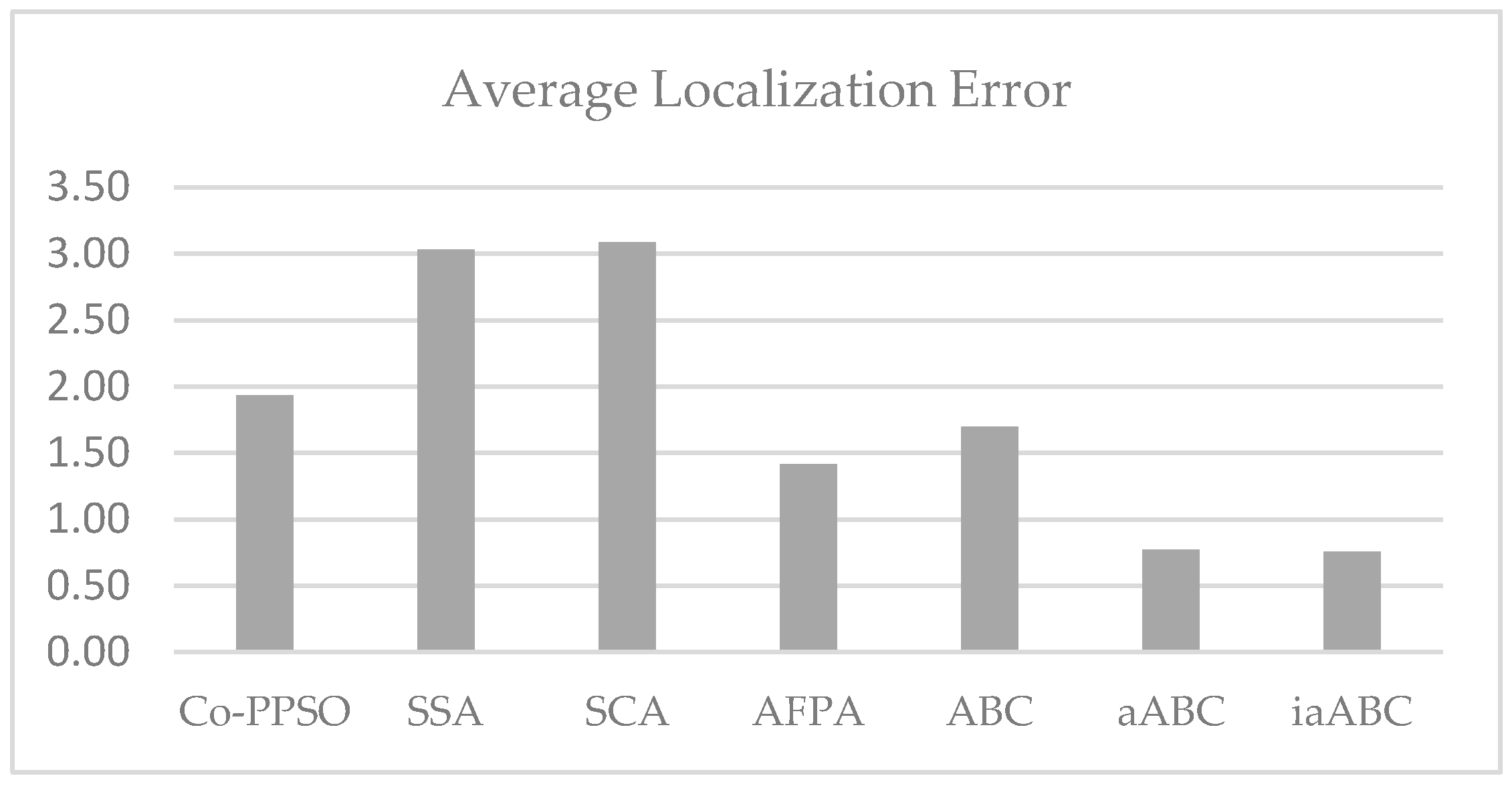
For the experiments conducted for the dynamic scenario, the minimum and maximum errors of the results produced by the competing algorithms and the calculated average error are presented in

Table 7. Comparison of algorithms.

Algorithms	Number of Movements	Localization Error (Max)	Localization Error (Min)	Average Error	Number of Located Targets
Co-PPSO	1	4.3710	0.0908	1.8458	100
	2	5.7293	0.1193	1.7638	100
	3	6.2017	0.1974	1.9267	100
	4	6.7341	0.1857	2.1561	100
	5	6.8199	0.1578	1.9744	100
SSA	1	4.7991	0.1056	2.2259	100
	2	6.3454	0.1774	2.6891	100
	3	6.8973	0.2119	2.4918	100
	4	8.3892	0.3272	3.9007	100
	5	7.2594	0.2805	3.8585	100
SCA	1	4.5295	0.1008	2.1722	100
	2	6.2578	0.1617	2.7114	100
	3	8.5904	0.2089	3.1056	100
	4	8.4899	0.3168	3.8873	100
	5	7.9741	0.2041	3.5671	100
AFPA	1	4.2779	0.1011	0.9861	100
	2	5.4338	0.0977	1.2391	100
	3	7.1194	0.1191	1.4468	100
	4	6.7734	0.0855	1.7348	100
	5	6.4891	0.0958	1.6814	100
ABC	1	4.3911	0.1148	1.1328	100
	2	6.0124	0.1067	1.3045	100
	3	7.1842	0.1247	2.2559	100
	4	7.0528	0.1163	1.8309	100
	5	6.8703	0.1189	1.9671	100
aABC	1	4.5803	0.0914	0.7832	100
	2	5.2579	0.1011	0.8011	100
	3	5.7711	0.0933	0.7546	100
	4	6.9016	0.0754	0.7949	100
	5	6.4715	0.0994	0.7284	100
iaABC	1	4.1107	0.0811	0.9993	100
	2	5.3199	0.1181	0.8597	100
	3	5.5551	0.0733	0.6311	100
	4	5.6916	0.0848	0.6882	100
	5	5.4157	0.0969	0.6118	100

and Figure 14.

Table 7 contains the errors calculated for the results obtained by the competitive algorithms for each experiment. Figure 14 displays the average error values for these experiments. A review of Figure 14 reveals that the proposed method yields results with generally lower errors.

The average processing time spent by the competitive algorithms for 30 experiments is shown in Figure 15. The processing time is presented in seconds and milliseconds.

6. Conclusions and Future Work

In WSNs, one of the most prominent topics of investigation is the localization problem. Localization in 3D WSNs has gained significant attention from researchers due to the expanding range of real-time applications for sensor networks. This is particularly relevant in static scenarios within a two-dimensional environment, where both range-based and range-free localization techniques are commonly employed to locate target nodes. This study focuses on a single anchor node approach, detailed in [11], specifically applied to three-dimensional WSNs. The main objective of the approach is to design the most effective umbrella projection using one anchor node and its virtual nodes to determine the locations of mobile TNs in a 3D environment. To achieve this objective, metaheuristic methods are utilized.

In this study, the iaABC algorithm is proposed for localization in a 3D WSN. This method is an improved model of adaptive ABC with an effective exploitation strategy to determine the search direction. In the adaptive version, the algorithm’s control parameters are updated to enhance exploitation, while in the improved model, the search direction is influenced by previous experiences. The statistical performance of iaABC was initially tested on the CEC 2022 test suits by comparing it with state-of-the-art algorithms. The results proved that the algorithm can successfully scan the solution space of the problem and has strong robustness. The method was later used to find TNs, and it was proven to achieve better results than other algorithms.

In particular, analyzing the data in Figure 15, it becomes clear that the standard ABC algorithm is very fast in generating solutions for numerical optimization problems. ABC is the second fastest algorithm after the SSA. Overall, it is thought that aABC is a version of standard ABC that increases the exploitation success but slows down the speed of producing solutions. Additionally, iaABC produces better solutions than both standard ABC and aABC, but it is slower in execution. Therefore, it can be concluded that iaABC may be the preferred option for 3D WSNs where time constraints are not critical.

In the next study, the method is planned to be applied in a real-world environment. Identifying the locations of robots and the density of diseased plants in a wide and rugged land where plant spraying robots operate is an important study topic in terms of agriculture. With the proposed method, a more efficient result is planned for plant irrigation, spraying, and monitoring.