1. Introduction
Overloading is a key issue and difficult point in the management of highway freight vehicles, while the traditional truck scale requires vehicles to wait in line, stop, and weigh, which often leads to congestion at the toll stations [
1,
2]. With the increasing demand for highway freight transportation in China, weigh-in-motion (WIM) technology, which enables accurate weight measurement while vehicles are in motion, is becoming increasingly important and has been developed rapidly. This technology holds notable research significance and engineering application value.
The goal of WIM systems is to obtain the number of axles and gross vehicle weight after the vehicle travels through WIM sensors at a constant speed. The advantage lies in the high traffic efficiency, whereas the challenge is to ensure weighing accuracy [
3,
4]. Currently, WIM systems are primarily divided into axle-load measurement and whole-vehicle-load measurement. Axle-load measurement weighs the individual axle loads to obtain the gross vehicle weight [
5]. The accuracy is generally improved by changing the sensor type [
6], optimizing the sensor layout [
7], and improving the weighing algorithm [
8]. For example, in 2011, Zhaojing Tong et al. proposed a WIM system based on a multi-sensor and Radial Basis Function (RBF) neural network. The proposed system shortened the testing time and improved the accuracy [
9]. When a vehicle is in motion, the axle loads change constantly as the center of mass moves. Therefore, the method of calculating the gross vehicle weight by weighing the axle loads at different times has defects in the weighing principle, which limits the improvement in the weighing accuracy of axle-load measurement and leads to untraceable weighing results.
Compared with axle-load measurement, whole-vehicle-load measurement has a significant improvement in weighing accuracy. For example, in 2017, Li Hailong et al. [
10] proposed a whole-vehicle-load measurement algorithm based on a Back Propagation (BP) neural network. This algorithm corrected the weighing signal by combining the axle type, speed, and acceleration, resulting in a weighing error of less than 0.5%. However, it does not support weighing multiple vehicles traveling through platforms simultaneously, and the traffic efficiency is low. At present, most whole-vehicle-load measurement systems using a large-platform scale still face the challenge of calculating the number of axles and the load of the individual axle [
11]. To identify the number of axles, most whole-vehicle-load measurement systems are equipped with axle recognition devices [
12], which increases the cost and reduces the system’s reliability due to the high failure rate of these devices. In 2015, Li Jianbo et al. [
13] used an expert algorithm to segment the entire weighing process of the vehicle, calculated the number of axles, and realized whole-vehicle-load measurement, but did not perform a quantitative analysis of axle recognition and weighing results.
In summary, whole-vehicle-load measurement has a higher accuracy. Furthermore, the axle load change caused by vehicle acceleration and deceleration will not affect the gross vehicle weight in whole-vehicle-load measurement. Then, whole-vehicle-load measurement has better robustness for vehicles traveling at variable speeds.
Consequently, this paper proposes a new modular WIM system that enables accurate axle recognition and weighing while multiple vehicles travel through platforms simultaneously. First, a new sensor module structure is designed, in which multiple scales are cascaded to create a combined scale, and each scale can be used independently or in combination. Second, instead of relying on specialized axle recognition devices, axle recognition is performed directly using the weighing signal from the WIM sensors. Therefore, an axle recognition algorithm based on a Transformer–Gated Recurrent Unit (GRU) is designed to classify the weighing signal at each time point and output the recognition results. Thus, the axle recognition task is converted into a sequence-to-sequence learning task, allowing the model to output the number of axles and the time points of axle entering and exiting platforms. This allows for determining the weighing time of both the axle and the whole vehicle to calculate the axle loads and gross vehicle weight.
Transformer is a deep learning model primarily used for natural language processing and sequence generation. It captures the relationships between different parts of the input data through the self-attention mechanism, making it particularly suitable for processing long sequence data. GRU is an improved version of the recurrent neural network, designed for sequence data processing. The Transformer part effectively captures global information and long-term dependencies, while the GRU part further captures local features, making it better suited for handling long sequence data with local information.
Finally, the accuracy of the axle recognition algorithm was tested on the test set and highway toll station. Additionally, the accuracy, consistency, and robustness of the modular WIM system were evaluated in the test field under different vehicle types, loads, and driving behaviors. The modular WIM system proposed in this paper has the advantages of high recognition, weighing accuracy, and traffic efficiency while meeting the requirements for accuracy, consistency, and traceability in measurement work. It is highly significant for implementing free-flow tolling and managing overload, in addition to presenting broad application prospects.
2. Materials and Methods
2.1. The Method of Transformer-GRU Model
Axle recognition is an important part of the WIM system, which is used to obtain the number of axles and the time points of entering and exiting platforms for each axle to obtain the gross vehicle weight. At present, most whole-vehicle-load WIM systems need to add axle recognition devices in the traveling direction, which increases the cost. Furthermore, the traditional peak detection algorithm [
14,
15] is easily influenced by interference signals, and the filtering and denoising processing [
16,
17] can affect the phase of the signal, leading to inadequate accuracy in detecting the start and end weighing time points. At present, deep neural networks have been successfully applied in Electrocardiography signal peak seeking and power quality disturbance signal recognition. Therefore, this study uses a deep neural network to accomplish the task of axle recognition. In this paper, an axle recognition algorithm based on Transformer-GRU is proposed to identify the axle directly by reasoning the weighing signal from the WIM sensors, which does not require axle recognition devices, reduces the cost, and enhances the system's reliability.
The architecture of the Transformer includes encoders and decoders, and realizes efficient information processing through a self-attention mechanism and fully connected layer. The self-attention mechanism enables the model to flexibly capture long-term dependencies in the input sequence, while multi-head self-attention allows the model to focus on information in parallel across different subspaces, thus efficiently processing long sequence data. Furthermore, the residual connection and layer normalization techniques in the model enhance stability and can better analyze the key information of the weighing signal. However, they may not fully capture the sequential local information in the sequence [
18]. To overcome this limitation, a GRU decoder was used to reconstruct the original sequence order.
By introducing reset gates and update gates [
19], the GRU provides the network with more flexibility to selectively forget or retain previous information. The reset gate determines which history information can be discarded, while the update gate regulates how the hidden state is updated using the candidate hidden state, which incorporates both historical information and the current time step data. GRU solves the problem of gradient disappearance in traditional recurrent neural networks (RNNs) by gating mechanism. Compared with Long Short Term Memory (LSTM), the GRU has a simpler structure and easier convergence.
In this paper, we propose a sequence-to-sequence model-based Transformer-GRU to generate 0–1 sequences for axle recognition and time positioning.
Figure 1 shows the overall architecture of the proposed sequence-to-sequence model, which consists of an input layer, a Transfromer encoder, a GRU decoder, and an output layer.
The input layer is mainly responsible for preprocessing the original data, including the vehicle entering and exiting platforms weighing signals collected by the WIM sensors. After standardization and labeling, we can obtain the input sequence and label sequence for the model.
The input sequence is fed into the Transformer encoder layer, which first embeds the input sequence and adds it with the positional encoding. Then, it is fed into the encoder, which is usually stacked with multiple independent coding layers. In this paper, we use a straightforward one-layer structure. The encoder layer consists of a multi-head self-attention mechanism and a fully connected feedforward network. A residual connection is adopted around the two sub-layers, and the activation value of each layer is normalized. Finally, a feature sequence with the same dimension as the input signal is obtained through the fully connected layer.
The feature sequence is sent to the hidden layer in the GRU decoder. The hidden layer consists of multiple stacked GRU layers, and the output of each GRU layer serves as the input for the next GRU layer. The output of the last GRU layer can be regarded as the feature extracted by the input sequence through the hidden layer in the current time step, and m is the number of neurons in the GRU layer.
The output layer receives the feature sequence extracted from the hidden layer. After traveling through the fully connected layer and sigmoid activation function, we obtain the output sequence . We binarize the output sequence to obtain a 0–1 sequence, which allows us to determine the class of each element, thereby identifying the corresponding weighing time points and the number of axles.
2.2. The Method of Modular WIM Systems
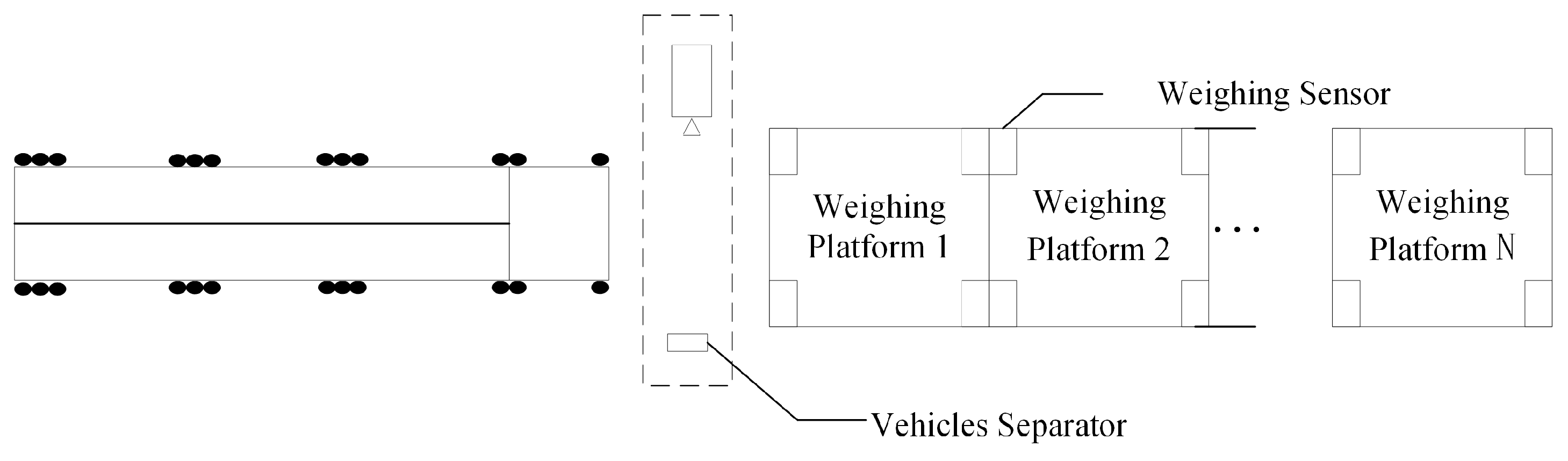
The modular WIM system consists of three main parts: a sensor module to obtain weighing signals, a data acquisition module to send signals, and a master control module to calculate the number of axles, axle loads, and gross vehicle weight. The innovative design of the sensor module is a key feature that makes the modular WIM system different from other WIM systems. Its structure is shown in
Figure 2. Along the traveling direction of the vehicle, there are a vehicle separator and N groups of weighing platforms, and each weighing module contains four bridge strain weighing sensors installed at the four corners of the platform. Weighing platforms operate independently, meaning that each platform can weigh on its own, or that multiple connected platforms can be combined to achieve weighing. The cascade structure design can help achieve two goals: one is continuous weighing with multiple vehicles traveling through platforms simultaneously, and the second is the whole-vehicle-load measurement of common vehicles.
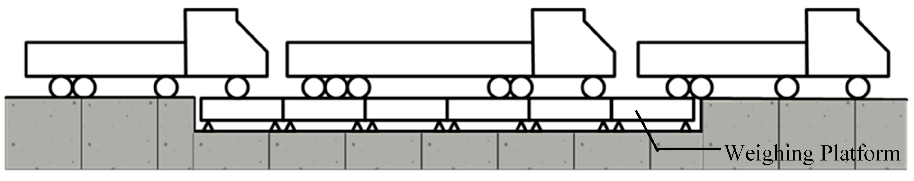
To enable continuous weighing with multiple vehicles traveling through platforms simultaneously, each weighing platform is designed to be 3.6 m, configured in a cascade structure. Thus, the probability of different vehicles having axles on the same weighing platform is low. The system uses a vehicle separator to obtain the occupied platforms for vehicles, enabling the combination of WIM sensor signals. Each vehicle is weighed on the platform it occupies without interference, thereby significantly improving the traffic efficiency of freight vehicles at toll stations. The schematic of the vehicle's continuous weighing with multiple vehicles traveling through platforms simultaneously is shown in
Figure 3.
By changing the number N of the weighing platforms, the total length of the weighing platform is adjusted to realize whole-vehicle-load weighing. Typically, the number of weighing platforms N ≤ 6. When N = 6, the total length of the weighing platform is 21.6 m, which exceeds the length of the conventional trucks. This configuration ensures sufficient weighing time for each vehicle while enhancing the weighing accuracy.
Simultaneously, on the master control module, the effective weighing signal is a step and stabilization process, as shown in
Figure 4b. As each axle enters and exits the scale platform, the signal increases and decreases, respectively. Therefore, it is essential to determine the time points of each axle entering and exiting the scale platform. Traditional methods include the slope segmentation algorithm based on Kalman smoothing and single most likelihood replacement. In this paper, we use an algorithm based on the Transformer-GRU Model to measure time points, and then obtain the number of axles and the gross vehicle weight.
2.3. The Measuring Method of Modular WIM System Based on Transformer-GRU
2.3.1. Axle Recognition
To calculate the number of axles, axle loads, and gross vehicle weight, it is necessary to obtain the signal of axle entering platforms from sensors in the front and the signal while exiting platforms from sensors in the rear as shown in
Figure 4a. The entering input sequence shows that when an axle enters the platform, there is a sudden change in the entering signal, and as the axle travels further away from the sensor, the signal gradually decreases; the exiting input sequence shows that when an axle exiting the platform, the change is the opposite. With the help of the Transformer-GRU axle recognition model identifying the time points of each axle entering and exiting the weighing platforms as the label sequence, the number of consecutive segments of class 1 in the label sequence is the number of axles, as shown in
Figure 4a, and it is a four-axle vehicle.
2.3.2. Weight Measuring
The part of axle loads and gross vehicle weight are accurately located in
Figure 4b. For example, for a four-axle truck, the input sequence and the ideal output sequence of the axle recognition model are shown in
Figure 4a. In
Figure 4b, the axle recognition signal which comes from
Figure 4a, and the weighing signal with multiple weighing platforms are drawn. Although the three signals come from different sensors, they maintain the same time scale, allowing the recognition results of the entering and exiting signal to be related to the weighing signal, and reflecting the position change in the vehicle on the platforms under different sampling points.
From
Figure 4b, it can be seen that axle 1 starts weighing at time point 1 and stabilizes at time point 2; axle 2 starts weighing at time point 3 and stabilizes at time point 4. Therefore, the weighing signal between point 2 and point 3 is the load of axle 1, and that between point 4 and point 5 is the loads of the sum of axles 1 and 2. At time point 6, axle 6 is completely on the scale, and axle 1 stops weighing at time point 7, therefore, the weighing signal between point 6 and point 7 is the gross vehicle weight. Similarly, the weighing signal of other individual axles or axle clusters can be determined.
When calculating the mean weight between point 6 and point 7, the signal that contains noise is first denoised based on Variational Mode Decomposition (VMD). VMD is used to decompose the signal into multiple Intrinsic Mode Functions (IMFs), and then find a set of K IMFs to minimize the residual between the original signal and their linear combination [
20]. To achieve the parameter self-optimization of VMD, the central frequency method [
21] is used to determine the mode decomposition number K, and sample entropy (SE) is introduced to identify effective modal components and noise modal components. After extensive testing, the SE threshold is set at 0.5, and the low-frequency IMF component with sample entropy values below this threshold is retained. A smooth denoising signal is obtained by reconstructing the low-frequency IMFs. The first and last maximum points in the signal are identified as the starting and ending points, respectively, for calculating the average value as the weight.
3. Results and Discussion in Axle Recognition
The axle recognition model was constructed using Transformer-GRU to locate the time points of axle entering and exiting platforms so as to calculate the number of axles, axle loads, and gross vehicle weight [
22,
23,
24,
25]. The input sequence was the weighing signal collected by the WIM sensors, and the label sequence was the 0–1 sequence, where the output value 1 represented the time points when the axle entered and exited platforms.
3.1. Training Process
3.1.1. Vehicle Data Acquisition and Selection
To facilitate field testing and verification, a modular WIM system was installed at the entrance lane of the Epang Palace highway toll station in Xi’an, Shaanxi, China. Approximately 1800 vehicles traveled through the lane every day, and we collected data from both rainy and sunny days. The weighing signals of 10,000 vehicles were randomly selected as the training and verification sets of the axle recognition model, and the weighing signals of 1853 vehicles were used as the test set. The dataset included multiple axle configurations, such as two-axle passenger cars, two-axle to six-axle trucks, and a small number of ultra-long trucks with more than six axles with extreme weight, achieving comprehensive coverage of vehicles at highway toll stations.
As shown in the sensor module structure diagram in
Figure 2, WIM sensors were installed at four corners of each weighing platform. The sum of the four sensors was referred to as the weight in one platform, the sum of multi-platforms occupied by vehicles was referred to as the combined weighing signal, the sum of the two sensors in front was referred to as the entering weighing signal, and the sum of the two sensors in the rear was called the exiting weighing signal. Weight fluctuations were obvious in the entering and exiting weighing signals. Therefore, the entering and exiting weighing signals were selected for axle recognition.
Figure 4a shows the entering and exiting weighing signals and the recognition results.
3.1.2. Standardized Processing of Data
The vehicle was separated according to the output signal of the light curtain separator, and the corresponding weighing signal of each vehicle was obtained. To ensure the consistent scaling of the model’s input signals and to enhance the training stability, the vehicle weighing signal was first normalized according to (1).
where
is the weighing signal, and
is the signal after being normalized.
And then signals were standardized using a z-score as described in (2).
where
is the mean of the signal and
is the standard deviation of the signal, and
is the signal after being standardized.
3.1.3. Data Annotation
We generated a label sequence that matched the length of the input sequence, where class 1 was assigned to the positions surrounding the axle key information, and class 0 was assigned to all the other positions. The consecutive segments of class 1 should begin when the axle starts entering or exiting the platform, until it has completely entered or exited the platform, to ensure that there is a sufficient segment length. The marked sequence represented the ideal output sequence of the model, and the axle signal corresponded to the class 1 segment with sufficient length, without generating noise from short class 1 segments, and ensured that no axle signals were missed. The ideal output signal is shown in
Figure 4a.
3.1.4. Training Optimization
To facilitate model training and testing, Pytorch was selected to construct sequence-to-sequence models based on Transformer-GRU.
Considering that there were only two classes, class 0 and class 1, in the target output sequence, the sigmoid activation function was added after the fully connected output layer to map the output value between 0 and 1, thereby accelerating the model’s convergence.
At the same time, since the number of class 0 in the label sequence was generally much more than the number of class 1, the focal_loss function was chosen to prevent the model from neglecting the learning of class 1, with an increased weight assigned to the class 1 and hard-to-classify samples. We do not want to lose class 1, so focal_loss helps the model avoid false negatives.
The Adam optimization algorithm was used during model training, gradient clipping was used to prevent gradient explosion, and L2 regularization was used to prevent overfitting.
The Transformer-GRU model was trained with the above conditions. The trend of training and validation loss is shown in
Figure 5. Since focal_loss dynamically adjusted the weight of hard-to-classify samples, validation loss fluctuated slightly, but both training loss and validation loss converged and the gap was small. The model was well trained and had high accuracy in testing.
Finally, the model was verified on the test set, and it was deployed at the Epang Palace highway toll station for field tests.
3.2. Test Set Results
Experimental analysis shows that a single Transformer encoder can extract the key information of the weighing signal, but the output signal cannot be calculated for the number of axles, the axle loads, and gross vehicle weight. Therefore, the GRU is necessary to decode the local information and obtain an ideal output. In addition, RNN and LSTM models were considered and compared when selecting GRU models.
To verify the accuracy of the axle recognition model based on Transformer-GRU, we used the test set for evaluation on a GTX 1080Ti GPU. The input was the weighing signal, the output was the time series of the same length as the input, and the output was binarized to obtain the 0–1 sequence. By post-processing the 0–1 sequence, we can calculate the number of segments of consecutive class 1 to obtain the number of axles. All the evaluation index metrics were calculated based on the number of axles. A total of 1853 vehicles were included in the test set. The confusion matrices of the Transformer-GRU model are listed in
Table 1. The distribution of vehicle types and the corresponding recognition performance under the Transformer-GRU model are listed in
Table 2.
The test set data simulated the number and proportion of vehicle types traveling through the highway toll station in a day, and appropriately increased the number of rare vehicles. Among them, the accuracy of all the vehicles reached 0.9951, the number of two-axle vehicles and six-axle vehicles was the largest, and the precision, recall, and F1-score all exceeded 0.99. In addition, vehicles with more than 6 axles were more susceptible to the influence of other vehicle types because of their lower number, with three false positives and two false negatives, but the precision, recall, and F1-score all exceeded 0.9. According to the confusion matrix, the false positives and false negatives were mainly caused by having one axle less or one axle more due to the recognition probability of a real axle being too low and the recognition probability of interference being too high, respectively.
Models based on Transformer-RNN, Transformer-LSTM, and Transformer-GRU were executed on a PC for comparative testing. The comparison of accuracy, training time with 200 epochs on a small dataset that contains 1134 vehicles, and average inference time for a vehicle among the three models are presented in
Table 3.
As shown in
Table 3, the sequence-to-sequence model based on Transformer-GRU exhibited the best performance on the test set with an accuracy of 99.51%. The Transformer-RNN model exhibited the worst performance with an accuracy of 75.07%. Compared with the Transformer-RNN model, the accuracy of the Transformer-LSTM model was improved by 19.84%. Furthermore, the RNN model had limited ability to process long sequences, which led to the loss of axle information and unsatisfactory recognition results. The introduction of the gating mechanism in the LSTM and GRU models can effectively solve the issues of vanishing gradients and exploding gradients of traditional RNN, although the training and testing time is increased, there were no special requirements on the hardware. This enhancement significantly boosted the accuracy of sequence-to-sequence models utilizing Transformer-LSTM and Transformer-GRU.
The LSTM model has a more complex network structure than the GRU models; therefore, it can capture contextual dependencies in sequences more effectively. However, the Transformer encoder already captured critical information of the weighing signal in long sequences, whereas the decoder needed to pay more attention to capturing the short and significant signal changes caused by instantaneous axle load fluctuations. The GRU controls the hidden state by integrating the forget and input gates into the update gates, and the structure was relatively simple with fewer parameters, faster training speed, and easier convergence, particularly when working with smaller datasets. Additionally, due to the varying lengths of weighing signals from different vehicles, the simple gating structure of the GRU models allowed them to adapt more flexibly to different timescales. These factors contributed to the Transformer-GRU model performing better on the test set compared with the Transformer-LSTM model.
3.3. Toll Station Field Test Results
To further verify the accuracy and robustness of the axle recognition model, the modular WIM system was installed at the entrance of Epang Palace highway toll station for field tests. The system included a data-collecting board and an upper computer. The data-collecting board obtained data from WIM sensors and transmitted them to the NVIDIA Jetson Xavier NX edge using an ethernet interface. And, the Transformer-GRU axle recognition model was deployed on the Jetson Xavier NX for a field test.
The speed of the vehicles in this toll station lane (
Figure 6) ranged from 0 to 30 km/h. In total, 9250 vehicles’ axle recognition results were recorded. The actual axle number was determined through a manual review, and the model results are presented in
Table 4.
The field test results showed that the accuracy is very similar between rainy and sunny days, and the accuracy improved by 0.33% compared with its performance on the test set. This improvement was primarily because two-axle and six-axle vehicles, which exhibited high accuracy with the Transformer-GRU axle recognition model, were the most frequently encountered at the toll station. The proportion of two-axle and six-axle vehicles had gradually increased, leading to a slight improvement in the model’s accuracy. In addition, although the operating conditions for trucks at the toll station were more complex, with various special situations such as parking and reversing, the five weighing platforms could identify five times and obtain voting results from the five sampling signals of one vehicle, further enhancing accuracy. The axle recognition model demonstrated strong accuracy and robustness when vehicles traveled through the toll station.
5. Conclusions
This paper proposes a modular WIM system, including an axle recognition algorithm based on the Transformer-GRU model and a weighing algorithm under the new sensor module, which realizes whole-vehicle-load weighing with multiple vehicles traveling through platforms simultaneously. It offers the advantages of high weighing accuracy, high traffic efficiency, and strong anti-cheating capabilities, enabling highway free-flow toll collection and overload management. Furthermore, the accuracy of the axle recognition algorithm based on Transformer-GRU achieves a very high level in both the test set and field test, offering advantages in reducing costs and enhancing system reliability. The verification of the five-platform modular system at the test site and toll station entrance shows excellent accuracy, consistency, and robustness. At present, modular sensor systems have passed the measurement organization evaluation test, and have been actually operated at toll stations in Guangxi, Yunnan, and Shaanxi, and the weighing results are accurate and reliable.


