Transforming Wind Data into Insights: A Comparative Study of Stochastic and Machine Learning Models in Wind Speed Forecasting

Abstract

Wind speed is a critical parameter for both energy applications and climate studies, particularly under changing climatic conditions and has attracted increasing research interest from the scientific comunity. This parameter is of interest to both researchers interested in climate change and researchers working on issues related to energy production. Based on this, in this study, prospective analyses were made with various machine learning algorithms, the long-short term memory (LSTM), the artificial neural network (ANN), and the support vector machine (SVM) algorithms, and one of the stochastic methods, the seasonal autoregressive integrated moving average (SARIMA), using the monthly wind data obtained from Bodo. In these analyses, five different models were created with the assistance of cross-correlation. The models obtained from the analyses were improved with the wavelet transformation (WT), and the results obtained were evaluated for the correlation coefficient (R), the Nash–Sutcliffe model efficiency (NSE), the Kling–Gupta efficiency (KGE), the performance index (PI), the root mean standard deviation ratio (RSR), and the root mean square error (RMSE). The results obtained from this study unveiled that LSTM emerged as the best performance metric in the M04 model among other models (R = 0.9532, NSE = 0.8938, KGE = 0.9463, PI = 0.0361, RSR = 0.0870, and RMSE = 0.3248). Another notable finding obtained from this study was that the best performance values in analyses without WT were obtained with SARIMA. The results of this study provide information on forward-looking modeling for institutions and decision-makers related to energy and climate change.

1. Introduction

The wind is a critical factor in the Arctic, particularly in Norway, as it drives the Arctic ecosystem, climate dynamics, and renewable energy production while the changing climate is reshaping the wind patterns, with significant implications for ecological systems, human communities, and energy projects [1,2,3]. Furthermore, as the Arctic continues to warm, the expected changes in wind patterns and their effects on oceanic and atmospheric processes will likely have cascading impacts on the environment and human activities [4]. In Norway, these shifts could influence fisheries, marine biodiversity, and hydrological systems, with far-reaching consequences for Arctic communities and industries dependent on these resources [5,6,7].

Accurate wind resource assessment and advanced forecasting techniques are critical for addressing these challenges and maximizing the potential of wind as a sustainable energy resource. Numerous methods have been applied to forecast wind separately or by a combination of stochastic methods, and machine learning. One prominent approach is the integration of machine learning with traditional statistical methods. For instance, Kim and Lee [8] propose a hybrid framework that combines long short-term memory (LSTM) networks with an unscented Kalman filter (UKF) to enhance wind nowcasting accuracy in aviation applications. This combination allows for better handling of the uncertainties inherent in wind data, demonstrating the effectiveness of hybrid models in forecasting tasks. Similarly, Xu and Yang [9] present a hybrid model that utilizes empirical mode decomposition (EMD) and multiple kernel Learning for short-term wind speed forecasting, showcasing the potential of combining different methodologies to improve prediction performance [9]. Haque et al. [10] also presented a hybrid machine learning technique composed of wavelet transform (WT) and fuzzy ARTMAP (FA) network for short-term wind speed forecasting.

The application of various machine learning algorithms has also been extensively documented. For example, Valsaraj et al. [11] analyze wind speed data with multiple ML techniques, including SVM, the multilayer feed-forward neural networks, and the adaptive neuro-fuzzy inference system (ANFIS), finding SVM to be the most effective. This aligns with findings from other studies, such as those by Fang and Chiang [12], who categorize forecasting methods into physical, statistical, and machine learning-based approaches, emphasizing the growing importance of ML in wind power forecasting. Furthermore, Demolli et al. [13] highlight using daily wind speed data with machine learning algorithms to forecast wind power, reinforcing the versatility of ML applications in this field. Khosravi et al. [14] developed multilayer feed-forward neural network (MLFFNN), support vector regression (SVR), fuzzy inference system (FIS), ANFIS, group method of data handling (GMDH) type neural network, ANFIS optimized with particle swarm optimization algorithm (ANFIS-PSO), and ANFIS optimized with genetic algorithm (GA), namely (ANFIS-GA), models to predict the time-series wind speed data.

Moreover, data-driven methodologies are increasingly recognized for their ability to leverage large datasets for improved forecasting. For instance, a study by Feng et al. [15] introduces a multi-model approach that employs deep feature selection to enhance short-term wind forecasting accuracy. This is complemented by the work of Yao et al. [16], who utilize LSTM networks to outperform other regression algorithms in forecasting wind power output based on real wind speed data. The integration of advanced data processing techniques, such as WT, has also been explored, as demonstrated by Zhang et al. [17], who employ extreme learning machines in their forecasting model. Alkesaiberi et al. [18] employed Bayesian optimization (BO) to optimally tune hyperparameters of the Gaussian process regression (GPR), SVR with different kernels, and ensemble learning (ES) models (i.e., boosted trees and bagged trees) and investigated their forecasting performance. The use of ensemble learning techniques has also gained traction in wind forecasting. Lee et al. [19] discuss the application of ensemble learning-based models to predict wind power, highlighting the advantages of combining multiple predictive models to enhance accuracy. This is further supported by Park et al. [20], who found that Gradient Boosting Regression Tree algorithms yield superior performance in forecasting wind power outputs compared to traditional methods. Heinermann and Kramer [21] investigated the use of machine learning ensembles for wind power prediction and proposed a heterogeneous ensemble approach utilizing both DT and SVR. Such ensemble approaches capitalize on the strengths of various models, leading to more robust predictions.

Along with the popular machine learning methods, the seasonal autoregressive integrated moving average (SARIMA) model stands out as a reliable method for wind speed prediction by effectively capturing seasonal trends and providing accurate forecasts essential for various meteorology and renewable energy management applications. Its adaptability and proven performance across different contexts make it a valuable tool for researchers and practitioners in the field. (SARIMA) model has emerged as a prominent statistical technique for wind speed prediction, mainly due to its ability to account for seasonal variations inherent in meteorological data. SARIMA extends the ARIMA model by incorporating seasonal components, making it particularly effective for time series data that exhibit periodic fluctuations, such as wind speed [22,23]. The model’s structure allows it to weigh historical observations differently, giving more importance to recent data, which is crucial for accurately forecasting rapidly changing environmental conditions [22].

Several studies have demonstrated the effectiveness of SARIMA in wind speed forecasting. For instance, Guo et al. [24] highlighted that the SARIMA model outperformed traditional ARIMA models in monthly wind velocity forecasting, showcasing its enhanced accuracy. Similarly, Tyass et al. [25] compared SARIMA with deep learning models and found that while both approaches have their merits, SARIMA remains a robust choice for wind speed prediction due to its statistical foundation and interpretability. Islam [26] applied long-term solar and wind resources estimation methods and indicated SARIMA as a powerful tool for prediction. However, he also notices the hyperparameter tuning and comprehensive understanding of data issues are challenging tasks with SARIMA. Furthermore, the model’s performance has been validated in various contexts, including large-scale wind farms, where it has been used to model uncertainty in wind speed forecasts [27]. The application of SARIMA is not limited to short-term predictions; it has also been effectively utilized for long-term forecasting of climatic parameters, including wind speed [22,23]. This versatility is particularly beneficial for energy production planning in wind farms, where accurate wind speed forecasts are critical for optimizing energy output and managing grid stability [28]. The integration of SARIMA with other forecasting techniques, such as neural networks, has also been explored, leading to hybrid models that leverage the strengths of both statistical and machine-learning approaches [29]. These hybrid models have shown promises in improving prediction accuracy, particularly in complex environments where multiple variables influence wind patterns [30].

This study evaluates and compares three advanced methodologies for wind prediction, integrating machine learning, signal processing, and stochastic techniques. Specifically, the stochastic approach employed in this study is the SARIMA model, which is assessed alongside machine learning techniques for their effectiveness and adaptability to diverse regional contexts in Bodø, Norway. The machine learning methods under investigation include LSTM: A type of recurrent neural network that excels at capturing long-term dependencies in sequential data, making it particularly effective for forecasting seasonally influenced variables like drought indices; SVM: A supervised learning algorithm adept at handling complex relationships between climate variables. Its robustness makes it well-suited for classification tasks and severity prediction, even with limited data availability; ANN: A model composed of interconnected processing units (“neurons”) that work collaboratively to model nonlinear patterns in data. To enhance the predictive performance of these methods, WT is employed as a preprocessing step. This versatile signal processing technique effectively captures both high-frequency and low-frequency patterns in climate data, thereby improving the input data quality for models such as LSTM and SVM.

The primary objective of this study is to determine the most effective machine learning algorithm and model architecture for describing wind speed at a monthly timescale. The performance of each method will also be evaluated in predicting maximum monthly wind speed. Moreover the study investigates the impact of data feature selection and the application of signal decomposition techniques in improving the accuracy and computational efficiency of wind speed forecasting. Through a comparative analysis of these approaches, this study aims to improve wind forecasting capabilities and offer practical insights in selecting the most effective methodologies across varying regional and climatic conditions.

2. Methodology

2.1. Study Area and Dataset

The study encompasses the Bodø region in Norway (Figure 1). Norway’s climate is predominantly maritime, strongly influenced by its latitude and extensive coastline, with the Gulf Stream bringing milder air to its shores. Bodø, with its proximity to the sea, experiences a more temperate oceanic climate, which can lead to varied precipitation patterns and influence drought frequency and severity. The Bodø region in Norway is characterized by its unique geographical, social, and cultural attributes, which collectively shape the experiences of its inhabitants. Located in Nordland County, Bodø serves as a central hub for various services and interactions among diverse populations, including both native Norwegians and immigrants. The region’s infrastructure, comprising significant harbors and an airport, facilitates connectivity and access to essential services, thereby influencing the utilization of healthcare and social services in the area [31]. The complex topography of the Bodø region further influences local wind patterns. Studies have shown that the interaction between large-scale winds and local terrain can create significant variability in wind speeds and directions. This variability is particularly pronounced in regions with complex topography, such as fjords and mountains, which can channel and amplify wind flows [32,33]. Additionally, the presence of snow and other natural disturbances can modify the wind’s impact on the local environment, affecting both vegetation and forest dynamics [34]. Future projections suggest that climate change will continue to alter wind patterns in the Bodø region. Recent studies indicate a potential decrease in extreme wind speeds in northern Norway, while southern regions may experience an increase [35]. This shift could have profound implications for local ecosystems, infrastructure, and energy production, particularly as Norway seeks to expand its offshore wind capabilities. Maximum wind speed patterns can be seen in Figure 2. Data used for the study areas are given in

Table 1. Information of dataset.

Data	Number of Data	Initial Data	End of Data	Mean	Min. (m/s)	Max. (m/s)	Standard Deviation	Skewness
Maximum Monthly Wind Speed	492	January 1983	December 2023	17.66	9.3	29.3	3.25	1.15

.

A full-scale meteorological observatory is operated by the Norwegian meteorological office in Bodø (station ID: SN82290; variables: temperature, precipitation, snow, and wind). Additional information about the station, based on their station ID, can be obtained from the Norwegian Climate Service Center “https://seklima.met.no/ (accessed on 28 January 2025)”.

2.2. Feature Selection

In this study, 5 different models were created in the analysis by utilizing machine learning algorithms. While creating these models, we used auto-correlation and cross-correlation methods. Each model was created according to the values obtained from these methods and the results obtained are shown in Figure 3 and

Table 2. The structure of all models.

Model			Inputs			Output
M01					Wt-12	Wt
M02				Wt-11	Wt-12	Wt
M03			Wt-1	Wt-11	Wt-12	Wt
M04		Wt-2	Wt-1	Wt-11	Wt-12	Wt
M05	Wt-10	Wt-2	Wt-1	Wt-11	Wt-12	Wt

. According to the cross-correlation results, the input data that have the most impact on the output parameter are the t-12 lagged data. It is understood from these results that the most second effective parameters are the data t-11 and t-2 lagged. The results obtained from cross-correlation and auto-correlation are very close to each other. The input variables based on results obtained from both methods were created as in Table 2. Many methods can be used to determine the input variables and also the model diversity can be increased. In the preliminary analysis, many different data input combinations were tried and as a result, it was decided to use the model inputs given in Table 2. The input variables that gave negative results as seen in Figure 3 were not added to the input structure because they did not give effective results in the preliminary analysis. Considering Table 2, the t-12, t-11, t-2, and t-1 indicate lagged time for 12 months, 11 months, etc. For instance, t-11 shows the input from the lagged time of 11 months before the output variable’s time t. Both methods here were applied to the entire dataset, and no pre-processing was applied to the data. The most successful models were chosen for this study.

2.3. Artificial Neural Network (ANN)

An artificial neural network (ANN) is composed of basic processing units called neurons which interact with one another [36]. These neurons process input data and derive logical outputs, passing information between neurons according to their weights, leading to an output similar to organic/biological brain networks. The learning phase of the ANN involves adjusting these weights to enhance overall performance [37]. The input layer receives raw data and then transmits it through the network to the output layer. There are many types of ANNs that exist, categorized by their learning algorithms and architectures, such as multi-layer perceptron (MLP) and feed-forward neural networks. In this study, an ANN model with an MLP architecture trained using the Levenberg–Marquardt backpropagation method was utilized, owing to its proven efficiency in hydrological forecasting [38].

MLP is one of the most widely employed forms of ANN for various applications. MLPs typically include one input layer, one or more hidden layers, and one output layer [39].

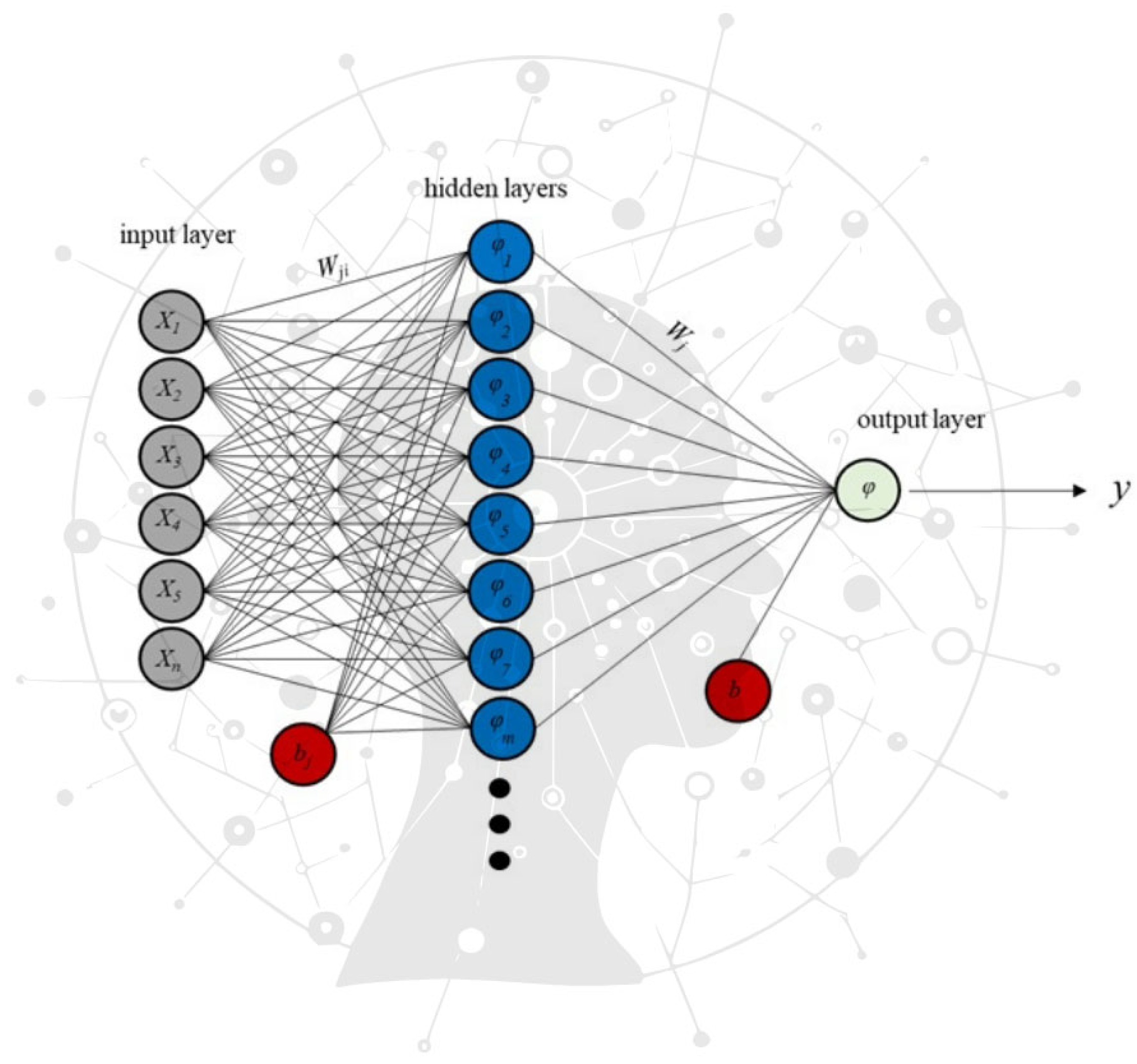
The topology of an ANN model, characterized by signals propagating layer by layer in a forward manner through the network, is concisely specified in Equation (1) and is illustrated in Figure 4 [40].

$$y=\left[{\sum }_{j=1}^m{w}_j\left({\sum }_{i=1}^N{w}_{ji}+b_j\right)+b\right]$$

(1)

where

• m: Number of neurons in the hidden layer.
• N: Number of samples in the input data.
• x_i: The ith input variable at time step t.
• w_ji: Weight connecting the ith neuron in the input layer to the ith neuron in the hidden layer.
• b_j: Bias term for the ith hidden neuron.
• ϕ_j: Activation function applied to the hidden neuron.
• w_j: Weight connecting the ith neuron in the hidden layer to the kth neuron in the output layer.
• b: Bias term for the kth output neuron.
• ϕ: Activation function applied to the output neuron.
• y: The predicted kth output at time step t.

This equation describes the forward propagation process in an ANN, where the input data are transformed through weighted summations, biases, and activation functions at each layer. The hidden neurons compute intermediate representations of the input data, while the output neurons produce the final predicted value $\left(y\right)$ for a given time step.

For additional foundational insights on ANN structures and functionality, refer to Kim and Valdés [39].

The calculations for the ANN in this study were performed utilizing MATLAB 2023a. The linear activation function was chosen for ANNs because of its superior performance compared to other functions, including logistic and sigmoid.

2.4. Support Vector Machine (SVM)

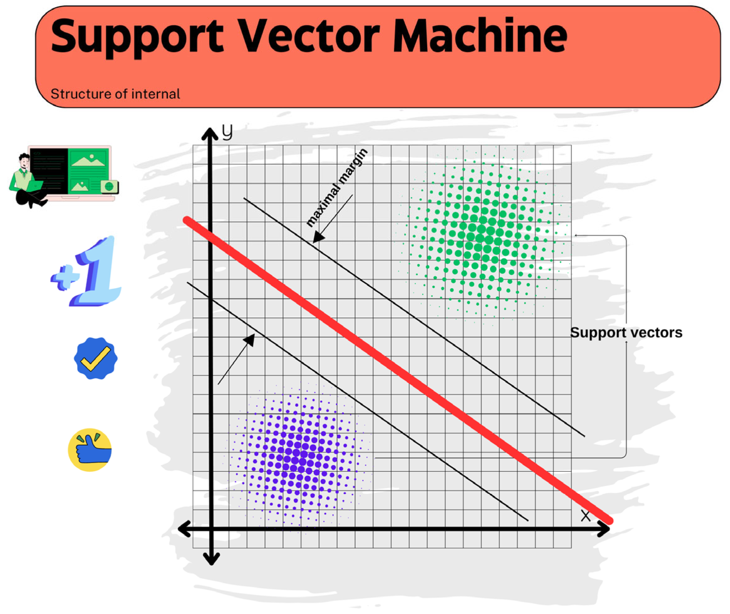
The works of Vapnik [41] paved the way for what would become known as support vector machines (SVMs), which were initially titled “Support-vector networks” [42]. SVM is extensively utilized for classification and regression, enhancing prediction accuracy in areas such as hydrology through statistical learning theory. SVM, as a supervised learning method, identifies a singular optimal solution for a given dataset, in contrast to other algorithms that may yield multiple potential solutions. This characteristic enhances its effectiveness in mitigating overfitting. This is achieved through the use of a kernel function that defines decision boundaries in nonlinear applications [43]. In the realm of kernel-based machine learning methods, SVM serves as a classifier aimed at categorizing data or predicting a fitness function through the minimization of classification errors or the fitness function itself. In linear data classification, the algorithm identifies a decision boundary that optimizes the margin between classes [44]. Figure 5 shows a sample of the SVM of the structure.

The versatility and robust performance of SVM in regression and classification tasks position it as a prominent method in machine learning, supported by numerous documented successful applications. Numerous modifications and enhancements to the fundamental SVM framework have demonstrated encouraging outcomes [45,46,47]. In the context of regression problems, SVM is known as support vector regression (SVR) [48,49]. The primary aim is to minimize statistical learning errors, which enhances the model’s predictive capabilities and robustness [50]. For further information regarding the theoretical foundations of SVR, refer to Gunn [51], Vapnik [41], and Panahi et al. [52]. The mathematical formulation of SVM is presented in Equation (2), defining the relationship between input and output variables:

$$f\left(x\right)=\left(w,\varphi \left(x\right)\right)+b$$

(2)

where $f\left(x\right)$ denotes a high-dimensional feature space, $w$ represents the weight of the output variable, and $b$ refers to the bias term.

2.5. Long-Short Term Memory (LSTM)

The long short-term memory (LSTM) networks improve upon standard recurrent neural networks (RNNs) by incorporating a mechanism that selectively retains or discards information via specialized memory cells and gates (Figure 6) [53]. The memory cells can retain information for prolonged periods, with the input, forget, and output gates regulating the data flow in and out [54,55]. LSTM effectively captures both short-term and long-term dependencies in the input. LSTM networks exhibit enhanced performance over conventional RNNs in tasks requiring long-term dependencies, effectively addressing the vanishing gradient problem. Success has been achieved in various applications, including video summarization [56], hand gesture recognition [57], and ship motion forecasting [58]. Furthermore, LSTMs have been integrated with other deep learning frameworks, including convolutional neural networks (CNNs), to develop hybrid models that effectively manage both spatial and temporal data [59].

An LSTM network is composed of a series of recurrently connected sub-networks known as memory blocks [60]. The blocks connect to the LSTM layer, which consists of units featuring an input gate, a forget gate, a cell with a self-recurrent loop, and an output gate [55]. These components dynamically add or remove information as required, a method first introduced by Hochreiter and Schmidhuber [53] and subsequently expanded by Gers et al. [61]. Various methods exist for optimizing LSTM parameters and reducing the loss function [55]. Similar to recurrent neural networks (RNNs), long short-term memory (LSTM) networks map an input sequence x to an output sequence y by iteratively computing the network unit activations from $t=1$ to $t=\tau$, with initial conditions $C_o=0$ and $h_o=0$. The LSTM computations are described by the following equations:

$$i_t=\sigma \left(W_i x_t+U_i h_{t-1}+b_i\right)$$

(3)

$$f_t=\sigma \left(W_f x_t+U_f h_{t-1}+b_f\right)$$

(4)

$$o_t=\sigma \left(W_o x_t+U_o h_{t-1}+b_o\right)$$

(5)

$$C_t=tanh\left(W_c x_t+U_c h_{t-1}+b_c\right)$$

(6)

$$C_t=f_t\otimes C_{t-1}+i_t\otimes C_t$$

(7)

$$h_t=o_t\otimes tanh\left(C_t\right)$$

(8)

where

Weight matrices: $W_i$, $W_f$, and $W_o$ represent the weights from the input to the input gate, forget gate, and output gate, respectively. Similarly, $U_i$, $U_f$, and $U_o$ denote the weights connecting the hidden layer to these gates.

Bias vectors: $b_i$, $b_f$, and $b_o$ are the bias terms associated with the input, forget, and output gates.

Activation functions: The sigmoid function ($\sigma$) serves as the non-linear activation applied element-wise, while the hyperbolic tangent (tanh) scales values between −1 and 1.

Gates and cell state: The vectors $i_t$, $f_t$, $o_t$, and $c_t$ correspond to the input gate, forget gate, output gate, and cell state at time step t, all of which are of the same dimension as the hidden state vector hth.

Element-wise operations: The symbol ⊗ denotes element-wise multiplication between vectors.

The LSTM network’s architecture uses these gates and the cell state to regulate the flow of information, enabling it to capture both long-term dependencies and short-term patterns effectively. For detailed analyses and further discussions on LSTM mechanisms, references such as Kratzert et al. [62], Zhang et al. [63], and Wang et al. [64] provide valuable insights.

Hyperparameters belonging to LSTM used in this study are as follows: hidden layers = (8, 16, 32, 64, 128, 256), solver = (Adam), step size = (96), and initial learning rate = (0.001, 0.3).

2.6. Seasonal Autoregressive Integrated Moving Average (SARIMA)

The seasonal autoregressive integrated moving average (SARIMA) model is a widely recognized statistical approach for forecasting time series data that exhibit seasonality and trends. Its structure is defined as SARIMA (p,d,q)(P,D,Q)S, where p, d, and q represent the non-seasonal autoregressive order, degree of differencing, and moving average order, respectively, while P, D, and Q correspond to the seasonal components of the model, and S denotes the seasonal period length [27]. The SARIMA model is particularly advantageous in fields such as epidemiology, economics, and environmental science, where seasonal patterns are prevalent.

$${\phi }_p(B){\Phi }_p(B^s)W_t={\theta }_q(B){\Theta }_Q(B^s){\omega }_t$$

(9)

The notation for Equation (17) is described as follows: The parameters p, d, and q represent the order of the non-seasonal components of the model. Specifically,

• P denotes the order of the seasonal autoregressive (AR) model.
• D refers to the number of seasonal differencing required to achieve stationarity.
• Q indicates the order of the seasonal moving average (MA) component.
• S represents the length of the seasonal cycle or periodicity.

In addition, ω_t refers to the white noise value at time t, while B denotes the backward shift operator. The SARIMA (p,d,q) × (P,D,Q)S model is particularly effective for analyzing a variety of time series due to its relatively compact order, making it computationally efficient. The periodicity ($s$) of the time series is determined based on the seasonal characteristics of the dataset.

One of the key strengths of the SARIMA model is its ability to capture linear relationships within time series data effectively. For instance, studies have demonstrated that SARIMA outperforms nonlinear models like back propagation neural networks (BPNNs) in forecasting disease incidence, as seen in the analysis of rubella incidence in Chongqing, China [65]. This finding is echoed in the context of mumps forecasting in Zibo City, where SARIMA exhibited superior performance compared to standard regression models, which often fail to account for autocorrelations and trends adequately [66]. Furthermore, the SARIMA model has been successfully applied to predict various infectious diseases, including tuberculosis and dengue fever, highlighting its versatility and reliability in public health forecasting [67]. However, the application of the SARIMA model is not without limitations. It is essential that the data used for modeling are relatively smooth, as the model may struggle with complex nonlinear data, potentially leading to a loss of information during the transformation process [68]. Additionally, while SARIMA is effective for many types of seasonal data, it may not always outperform hybrid models that combine SARIMA with other techniques, such as ANN or GA [69,70]. For example, a hybrid SARIMA-ANN model has shown improved forecasting accuracy in various studies, suggesting that combining different modeling approaches can enhance predictive performance [71,72].

In conclusion, SARIMA remains a robust method for forecasting seasonal time series data, particularly in fields requiring accurate predictions of trends and cyclic patterns. Its ability to model linear relationships effectively makes it a preferred choice in many applications, although researchers should remain cognizant of its limitations and consider hybrid approaches for more complex datasets. Continued exploration of SARIMA’s hyperparameters and its integration with other forecasting methods will likely yield further improvements in predictive accuracy across diverse domains [73,74]. The development of an ARIMA model involves three key stages: identification, parameter estimation, and diagnostic testing [75].

• Identification: This stage focuses on selecting the appropriate level of differencing to transform the time series into a stationary form. It also involves determining the desired order of the model and analyzing the autocorrelation function (ACF) and the partial autocorrelation function (PACF). These functions help to uncover the temporal correlation structure of the transformed data. Specifically:
  • The ACF is used to assess whether past values have a significant association with the current values.
  • The PACF quantifies the correlation between the variable and its time-lagged values, while controlling for intermediate lags.
• Model Selection: The Akaike information criterion (AIC) and the Bayesian information criterion (BIC) (also referred to as Schwarz’s BIC) are commonly employed to identify the optimal model. These criteria are defined mathematically in Equations (6) and (7), respectively, and provide a trade-off between model complexity and goodness-of-fit.
• Parameter Estimation and Diagnostic Testing: Once the model structure is identified, parameters are estimated, and diagnostic testing is performed to ensure the model adequately fits the data.

The $AIC$ and $BIC$ serve as key tools in balancing model parsimony with accuracy, enabling the selection of an effective ARIMA model [75].

$$AIC=-2\log \left(L\right)+2k=-2\log \left(L\right)+2(p+q+P+Q)$$

(10)

$$BIC=-2\log \left(L\right)+k \ast ln\left(n\right)=-2\log \left(L\right)+(p+q+P+Q)$$

(11)

In this context, n represents the number of observations in the time series, while k denotes the set of ARIMA parameters. Through empirical analysis, it was observed that the model’s efficiency improved as the $AIC$ value decreased. The forecasting model with the lowest $AIC$ score was identified as the best-fitting model, indicating its superior balance between complexity and goodness-of-fit [75,76].

In order to determine the most suitable model, many models are defined and among these, residuals are examined. Following the selection of the stochastic time series model, the stationarity and reversibility of the model parameters are examined. The most popular method among those suggested in the literature is to look at the residual terms’ correlogram (ACF) after testing them as independent series in order to choose the best model for explaining the process. The residual terms’ correlogram should be independent, random, and below a selected confidence level, which is often 95%. The model’s residual terms must be regularly distributed and independent of time. The Ljung–Box test [11], which is provided as follows, is used to verify it.

$$Q=n(n+2){\sum }_{k=1}^m{(n-k)}^{-1}{r_{k\left(e\right)}}^2$$

(12)

where m is the maximum lag, r_k(e) is the residual correlogram, and n is the number of observations. It is compared with the χ² (chi square) statistic, which is the degree of freedom (m-p-q) at a chosen significance level with the calculated Q statistic.

2.7. Wavelet Transformation (WT)

In the literature, wavelet transformations are typically categorized into two variants: continuous wavelet transformation (CWT) and discrete wavelet transformation (DWT). Discrete wavelet transformation (DWT) is frequently favored over continuous wavelet transformation (CWT) because of its reduced computational demands.

Discrete wavelet transform (DWT) serves as a signal processing technique and an alternative to the Fourier transform by decomposing time series data into independent sub-signals across various frequencies, thereby facilitating the identification of significant features [77,78,79]. By incorporating both temporal and spectral dimensions, it provides a thorough time-frequency analysis of the signal. The mother/main wavelet function is represented as $\psi y\left(t\right)$, which is the fundamental component of DWT, serves as a base function. This wavelet captures distinct frequencies by modifying different scales ($s_0$) and translating in time (${\tau }_0$), which allows for precise localization in the time-frequency domain. The formulation of the mother wavelet is expressed in Equation (13):

$${\psi }_{m,n}(t)={\displaystyle \frac{1}{s_0^m}}\psi \left\{{\displaystyle \frac{t-n{\tau }_0{s}_0^m}{s_0^m}}\right\}$$

(13)

where

$m$ and $n$ are integers representing the scale and shift parameters, respectively;

${\psi }_{m,n}(t)$ is the wavelet function.

Typically, the scale parameter $s_0$ is set to 2, and the shift parameter (${\tau }_0$) is set to 1. According to Mallat’s theory, DWT decomposes a signal into a series of approximation and detail components, which are linearly independent. In this framework:

• s₀ represents the precision step for the signal’s expansion.
• τ₀ denotes the localization parameter for handling discrete time series data ($x_i$), where the data are sampled at discrete intervals (i).

The inverse DWT, which reconstructs the original signal from its approximation and detail components, is defined in Equation (14), following the framework established by Mallat [80]:

$$x\left(t\right)=T+{\sum }_{m=1}^M{\sum }_{t=0}^{2^{M-m-1}}{W}_{m,n}{2}^{-{\displaystyle \frac{m}{2}}}\psi (2^{-m}t-n)$$

(14)

where $W_{m,n}{2}^{-{\displaystyle \frac{m}{2}}}{\sum }_{t=0}^{N-1}\psi \left(2^{-m}t-n\right)x(t)$ is the wavelet coefficient for the discrete wavelet at scale s = $2^m$ and τ = $2^m$. In this study, a 5-level decomposition was chosen for the wavelet transformation because it improved the model results. The calculation for the level is given by Equation (15):

$$L=int\left(N\right)$$

(15)

where $L$ is the level of the decomposition and $N$ is the number of runs.

2.8. Performance Metrics

There are various statistical performance measurement criteria in the literature. The created models were appraised to test the prediction accuracy of models with 6 different statistical methods: correlation coefficient (R), RMSE (root mean-square error), Nash–Sutcliffe efficiency coefficient (NSE), and Kling–Gupta efficiency (KGE).

The correlation coefficient (R) is given in Equation (16) [81]:

$$\mathrm{R}={\displaystyle \frac{\sum _{i=1}^N{(W}_{pi}-\overline{W_p})(W_{oi}-\overline{W_o})}{\sqrt{\sum _{i=1}^N{{(W}_{pi}-\overline{W_p})}^2} \ast \sqrt{\sum _{i=1}^N{(W_{oi}-\overline{W_o})}^2}}}$$

(16)

where $W_{pi}$ is predicted W for i, $\overline{W_p}$ indicates the mean of the predicted W value, $W_{oi}$ shows observed W values for i, and $\overline{W_o}$ indicates the mean of the observed W value.

RMSE is given in Equation (17) [81]:

$$\mathrm{R}\mathrm{M}\mathrm{S}\mathrm{E}=\sqrt{{\displaystyle \frac{1}{N}}\sum _{t=1}^N{\left(W_{oi}-W_{pi}\right)}^2}$$

(17)

NSE is sensitive to additive and proportional differences between forecasts and observations [82].

NSE is calculated in Equation (18):

$$\mathrm{N}\mathrm{S}\mathrm{E}=1-\left[{\displaystyle \frac{\sum _{t=1}^N{\left(W_{oi}-W_{pi}\right)}^2}{\sum _{t=1}^N{\left(W_{oi}-\overline{W_o}\right)}^2}}\right]$$

(18)

Gupta et al. [83] proposed the Kling–Gupta efficiency (KGE), which is based on the decomposition of the Nash–Sutcliffe efficiency [82] into its fundamental components: correlation, variability bias, and systematic bias, for the calibration and evaluation process of hydrological models.

$$\mathrm{K}\mathrm{G}\mathrm{E}=1-\sqrt{{({\alpha }_P-1)}^2+{({\beta }_P-1)}^2+{({\gamma }_{RP}-1)}^2}$$

(19)

$${\beta }_P={\displaystyle \frac{{\mu }_G}{{\mu }_O}}$$

(20)

$${\gamma }_{RP}={\displaystyle \frac{{CV}_G}{{CV}_O}}={\displaystyle \frac{\left(\frac{{\sigma }_G}{{\mu }_G}\right)}{\left(\frac{{\sigma }_O}{{\mu }_O}\right)}}$$

(21)

where ${\alpha }_P$ represents the Pearson correlation between the data observed and GCM-analyzed data, ${\beta }_P$ represents the bias rate, and ${\gamma }_{RP}$ represents the variability rate. In Equation (5), ${\mu }_G$ and ${\mu }_O$ represent the average of GCM-analyzed and observed data, respectively. In Equation (6), ${CV}_G$ and ${CV}_O$ represent the coefficient of variation of GCM-analyzed and observed data, respectively. KGE values range from minus infinity to 1; values closer to 1 indicate higher model performance.

Another method that used performance metrics for comparison is the RMSE-standard deviation ratio (RSR). This method’s calculation is as follows:

$$\mathrm{R}\mathrm{S}\mathrm{R}=\left[{\displaystyle \frac{\sqrt{\sum _{t=1}^N{\left(W_{oi}-W_{pi}\right)}^2}}{\sqrt{\sum _{t=1}^N{\left(W_{oi}-\overline{W_o}\right)}^2}}}\right]$$

(22)

3. Results

This study employed both stochastic method, SARIMA, and machine learning algorithms, ANN, SVM, and LSTM to model the wind speed data measured for Bodo in Norway. The results obtained from these techniques were further enhanced using WT, significantly improving the predictive accuracy and capability.. Using WT enabled a more detailed analysis of the data and captured patterns that were not evident in the raw data. Consequently, the overall accuracy of the predictions improved significantly, enhancing the reliability of the findings. These improvements contribute to more reliable forecasts that provides valuable insights for decision-makers against natural disasters or develop energy planning strategies in the region.

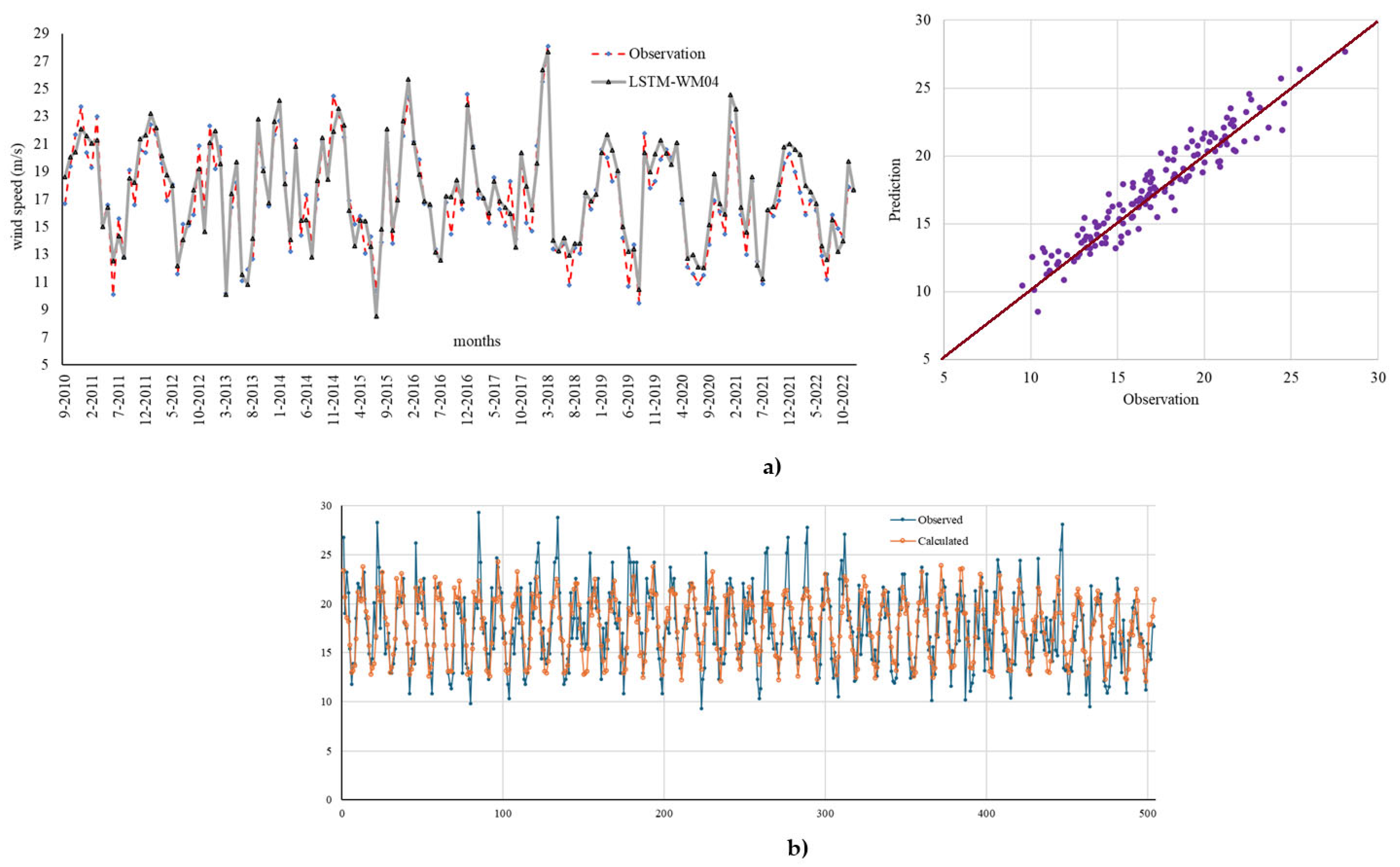
For this study, 70% of the monthly wind speed data from the study area was used for learning/training, while 30% was reserved for testing. The results from all techniques, both with and without WT, were shown in

Table 3. The results of all models and algorithms.

	LSTM						ANN						SVM
	R	NSE	KGE	PI	RSR	RMSE	R	NSE	KGE	PI	RSR	RMSE	R	NSE	KGE	PI	RSR	RMSE
M01	0.6087	0.2715	0.5612	0.1148	0.2289	0.8506	0.5161	0.2016	0.4562	0.1275	0.8905	3.3086	0.5451	0.2932	0.3992	0.1177	0.2255	0.8378
M02	0.6461	0.3678	0.5519	0.1045	0.2133	0.7924	0.5568	0.2617	0.4810	0.1194	0.8564	3.1816	0.5818	0.3340	0.4434	0.1116	0.2189	0.8133
M03	0.6511	0.3784	0.5466	0.1033	0.2115	0.7858	0.5717	0.2788	0.5195	0.1169	0.8464	3.1446	0.6120	0.3743	0.4613	0.1062	0.2122	0.7883
M04	0.4971	0.1613	0.1391	0.1323	0.2457	0.9127	0.5663	0.2021	0.5544	0.1234	0.8902	3.3075	0.6160	0.3792	0.4683	0.1055	0.2114	0.7853
M05	0.6511	0.3818	0.5910	0.1030	0.2109	0.7836	0.2182	−1.9460	0.0029	0.3048	1.7106	6.3554	0.6167	0.3787	0.4678	0.1055	0.2114	0.7856
	LSTM-W						ANN-W						SVM-W
	R	NSE	KGE	PI	RSR	RMSE	R	NSE	KGE	PI	RSR	RMSE	R	NSE	KGE	PI	RSR	RMSE
M01	0.6709	0.4055	0.5991	0.0998	0.2068	0.7684	0.5274	−0.0131	0.5238	0.1426	1.0031	3.7270	0.6754	0.4516	0.5858	0.0956	0.1987	0.7381
M02	0.6457	0.3305	0.6260	0.1076	0.2195	0.8155	0.1137	−0.5921	0.1034	0.2451	1.2575	4.6720	0.6775	0.4513	0.5976	0.0955	0.1987	0.7383
M03	0.9400	0.8646	0.9282	0.0410	0.0987	0.3667	0.4148	−1.5852	0.0588	0.2459	1.6024	5.9534	0.8453	0.7133	0.7745	0.0628	0.1436	0.5336
M04	0.9532	0.8938	0.9463	0.0361	0.0870	0.3248	0.2851	−1.0483	0.2104	0.2409	1.4263	5.2993	0.9289	0.8593	0.9276	0.0421	0.1006	0.3739
M05	0.9502	0.8820	0.9421	0.0381	0.0921	0.3423	0.4374	−1.0264	0.2224	0.2143	1.4187	5.2710	0.9296	0.8601	0.9270	0.0419	0.1003	0.3728
	SARIMA
	R	NSE	KGE	PI	RSR	RMSE
MR1	0.7411	0.5455	0.6745	0.0856	0.6735	2.6348
MR2	0.7153	0.5013	0.6543	0.0910	0.7055	2.7598
MR3	0.7186	0.4954	0.6859	0.0913	0.7096	2.7761
MR1:	(0,0,0)(8,1,0)12
MR2:	(1,1,1)(6,1,0)12
MR3:	(6,1,0)(8,1,0)12

Bolds represent the best results.

. Besides, in Table 3, the best results in each group are highlighted in bold. According to the results, the most successful model was M04 utilizing the LSTM algorithm with WT (LSTM-WM04). This model achieved the highest performance with R = 0.9532, NSE = 0.8938, KGE = 0.9463, PI = 0.0361, RSR = 0.0870, and RMSE = 0.3248, among all the results, including/incorporating input data t-1, t-2, t-11, and t-12. In contrast, without WT, the performance metrics for the same model were significantly lower (R = 0.4971, NSE = 0.1613, KGE = 0.1391, PI = 0.1323, RSR = 0.2457, and RMSE = 0.9127), demonstrating the improvements gained with WT. The M05 model with WT, also performed well, with metrics R = 0.9502, NSE = 0.8820, KGE = 0.9421, PI = 0.0381, RS = 0.0921, and RMSE = 0.3423. However, the input structure of these two models is different. Including a different input structure, t-10 lagged wind speed data, negatively impacted the performance of M05. Therefore, it can be concluded that the performance differences between these two models primarily depend on the selected input data. In the analysis performed without WT, it was observed that M05 outperformed the other models. Figure 7a shows a comparison of this model with observation values.

Another method used in this study for wind speed prediction is ANN. The analyses revealed that there was a decrease in performance metrics across all ANN models when WT was applied. Therefore, ANN with WT is not recommended to predict wind speed in this region. In the analysis performed without WT, however, the most successful ANN model was M03, yielding performance metrics of R = 0.5717, NSE = 0.2788, KGE = 0.5195, PI = 0.1169, RSR = 0.8464, and RMSE = 3.1446.

SVM is another machine learning algorithm used in this study. While the most successful SVM model in the analysis without WT was M04 (SVM-M04), whereas the most successful SVM algorithm in the analysis with WT was M05 (SVM-WM05). Although SVM-WM05 outperformed other SVM models, it still falls behind models LSTM-WM04, LSTM-WM05, and LSTM-WM03 in terms of performance. Overall, the application of WT improved the performance of all SVM models. However, compared to LSTM-based models, SVM models showed relatively lower performance.

Another forecasting method used for this study region is SARIMA, a stochastic model that also accounts for the seasonal effects. The findings from SARIMA are presented in Table 3. Besides, in this study, we created many models in the analysis with SARIMA. But we added the three most effective models, MR1, MR2, and MR3, these models estimated output value, which is the wind speed, in the best way, as performance metrics to the study. Among all SARIMA models, MR1 demonstrated the best performance metrics, achieving R = 0.7411, NSE = 0.5455, KGE = 0.6745, PI = 0.0856, RSR = 0.6735, and RMSE = 2.6348. When compared with machine learning algorithms performed without WT in terms of overall performance, MR1 ranked second, following LSTM-M05. Therefore, SARIMA (particularly MR1) is one of the preferred methods when WT is not applied in this region for wind speed forecasting. Figure 7b shows a comparison of this model with observation values. Three different SARIMA models (MR1, MR2, and MR3) were developed, each having distinct input structures, and their results are shown in

Table 4. (a) Summary of the selection of stochastic models. (b) SARIMA (0,0,0)(8,1,0)₁₂ model parameters and their probabilities. (c) Asymptotic correlation matrix of SARIMA (0,0,0)(8,1,0)₁₂ model.

(a)
Model			AIC		BIC		Log Likelihood
SARIMA (0,0,0)(8,1,0)12 (MR1)			992.5600		1026.3410		−488.2800
SARIMA (1,1,1)(6,1,0)12 (MR2)			1039.2921		1073.0730		−511.6460
SARIMA (6,1,0)(8,1,0)12 (MR3)			1057.2203		1116.3360		−514.6102
(b)
Model Estimation Section
Parameter	Parameter Estimate		Standard Error		T-Value		Prob Level
SAR (1)	−0.8007		0.0446		−17.9386		0.0000
SAR (2)	−0.7161		0.0543		−13.1831		0.0000
SAR (3)	−0.6014		0.0604		−9.9501		0.0000
SAR (4)	−0.5319		0.0611		−8.7065		0.0000
SAR (5)	−0.4948		0.0610		−8.1042		0.0000
SAR (6)	−0.4185		0.0592		−7.0708		0.0000
SAR (7)	−0.3718		0.0538		−6.9135		0.0000
SAR (8)	−0.1595		0.0449		−3.5508		0.0004
(c)
	SAR (1)	SAR (2)	SAR (3)	SAR (4)	SAR (5)	SAR (6)	SAR (7)	SAR (8)
SAR (1)	1.0000	0.6202	0.5012	0.3906	0.3343	0.3099	0.2599	0.2580
SAR (2)	0.6202	1.0000	0.7035	0.5497	0.4252	0.3553	0.2990	0.2431
SAR (3)	0.5012	0.7035	1.0000	0.7262	0.5755	0.4437	0.3573	0.3007
SAR (4)	0.3906	0.5497	0.7262	1.0000	0.7151	0.5455	0.3914	0.2916
SAR (5)	0.3343	0.4252	0.5755	0.7151	1.0000	0.6995	0.5216	0.3538
SAR (6)	0.3099	0.3553	0.4437	0.5455	0.6995	1.0000	0.6715	0.4741
SAR (7)	0.2599	0.2990	0.3573	0.3914	0.5216	0.6715	1.0000	0.6022
SAR (8)	0.2580	0.2431	0.3007	0.2916	0.3538	0.4741	0.6022	1.0000

and Figure 8.

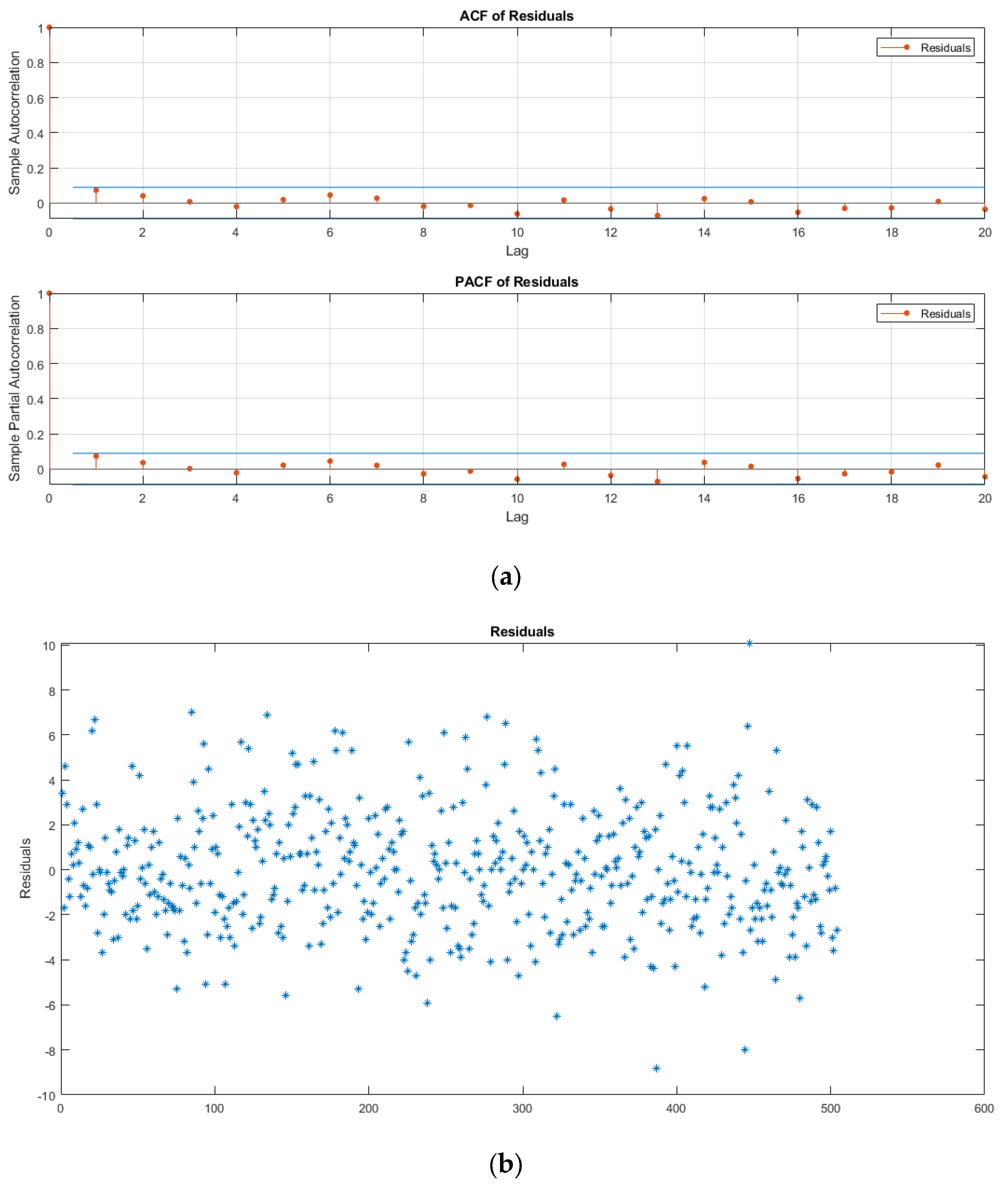
The time series model was systematically examined through three stages: identification, parameter estimation, and diagnostic checking. To construct an appropriate ARIMA model, it is essential for the time series to be stationary. The ACF and PACF plots for the wind data, presented in Figure 8, indicate the orders of the AR and MA components, along with skewness and noticeable significant deviations. Therefore, in this study, seasonal differencing was applied to ensure stationarity.

In this study, a stochastic SARIMA model was considered, and multiple SARIMA models were tested to determine the best-fitting model. Based on the AIC and BIC criteria, the optimal SARIMA model was identified as SARIMA (0,0,0)(8,1,0)₁₂. Table 4a presents some of the tested models along with their corresponding AIC and BIC values. The parameters of the selected best-fitting model are provided in Table 4b,c. Specifically, Table 4b lists the model parameters along with their probabilities of being the best fit. Since all p-values are below 5%, this confirms the statistical significance of the parameters. Additionally, Table 4c displays the asymptotic correlation matrix for the selected model parameters, further supporting the robustness of the chosen model.

Figure 8a depicts the residuals’ ACF and PACF, revealing no significant lags and suggesting that the residuals behave as white noise. Figure 8b illustrates the variation of these residuals, indicating independence. Additionally, the Ljung–Box test was conducted up to fifty lags, achieving probabilities exceeding 5%, which confirms that the residuals are uncorrelated and independent and validates that the selected model is an appropriate model.

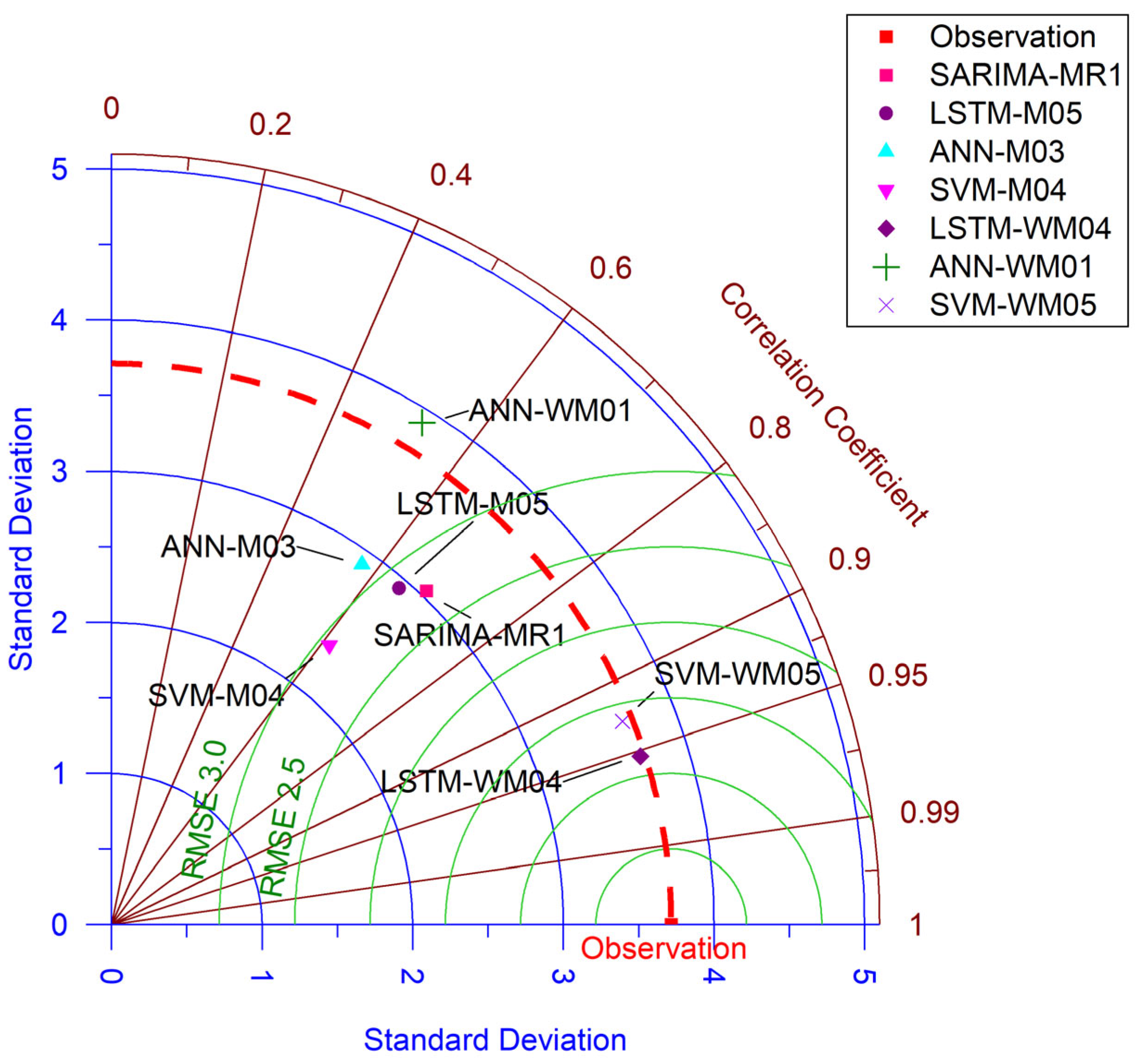
A Taylor diagram was used to compare the most successful methods within their respective categories among all the methods analyzed (Figure 9). According to the results, the LSTM-WM04 model is the closest to the observed values compared to other models. Additionally, as shown in Table 3, this model achieves the best performance metrics among all algorithms and models. The consistency between the results obtained from these two different evaluation methods further reinforces the reliability of the findings.

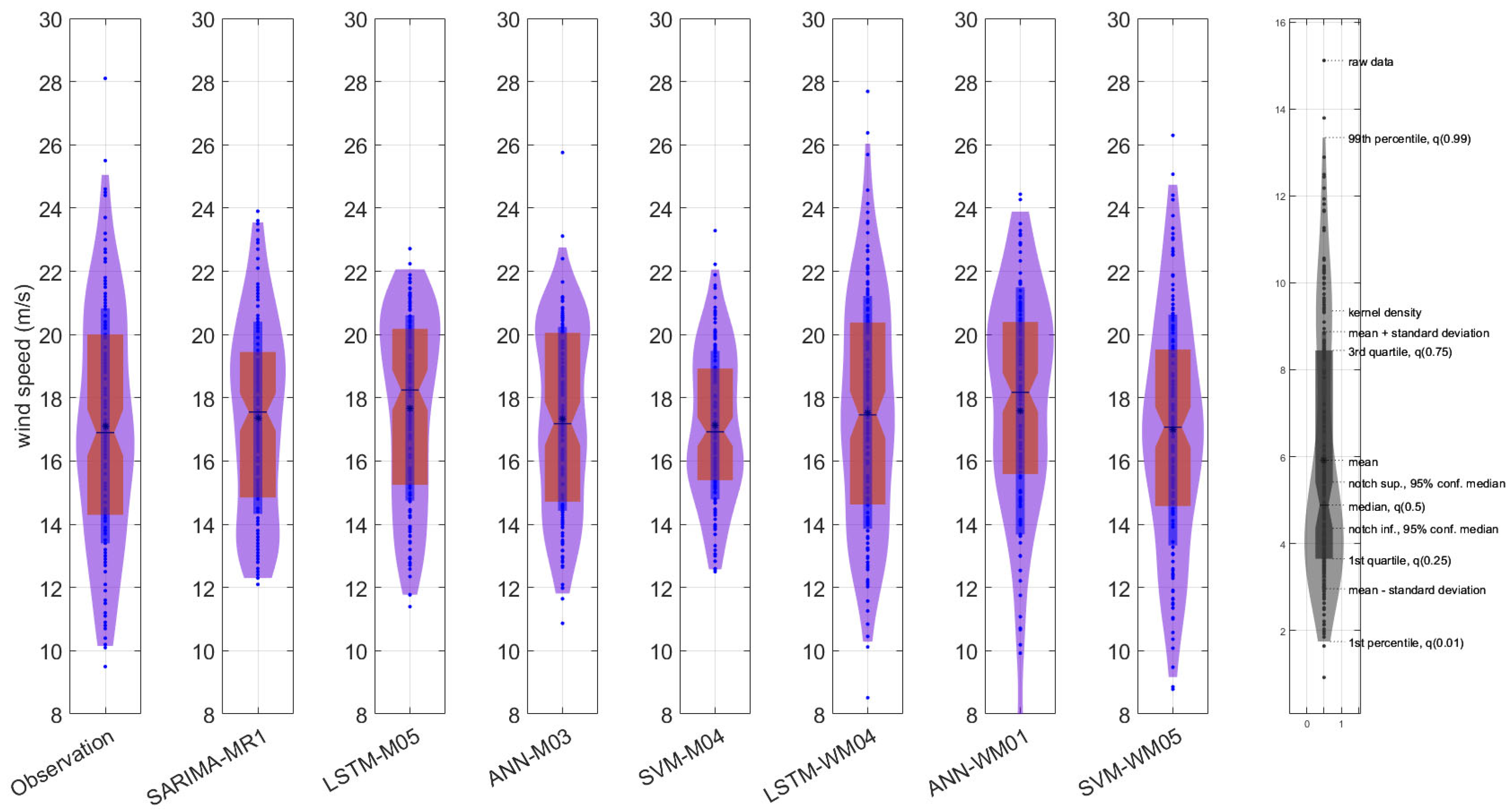
The Violin diagram, a method used to compare performance metrics between models, is also employed in this analysis. The results from this diagram, shown in Figure 10, indicate that the LSTM-WM04 model closely exhibits the observation values in shape. The results from this model show the most accurate representation of the extreme values found in the observation data. Moreover, the mean and median values of the LSTM-WM04 models are closely aligned with the observed values while the kernel density as well as the 1st and 3rd quartiles also show strong agreement with the observation values. The SVM-WM05 model exhibits a similar performance, closely following the observation values. Overall, the findings from the Violin diagram are consistent with the statistical results, reinforcing the robustness of the analysis.

The Ridge chart was also used to compare the performance of models (Figure 11). In this chart, the most successful models within their respective categories are compared against each other. Based on the results of the Ridge chart analysis, the LSTM-WM04 model demonstrates the highest similarity to the observed values, particularly in terms of peak alignment. The peaks of this model closely correspond to those of the observed values, indicating strong agreement. In contrast, the SVM-M04 and ANN-WM01 models exhibit shapes that are noticeably different from the observed values, suggesting lower performance in capturing the observed patterns.

4. Discussion

In this study, the most suitable model and algorithm for predicting future wind speed were identified by applying a series of machine learning algorithms alongside SARIMA, a stochastic method, using monthly measured wind speeds in the Bodo region. The findings of this study align with results from previous research in the literature.

For instance, Karaman [84] modeled wind energy data from a wind turbine located in the Şenköy region using LSTM, ANN, the recurrent neural network (RNN), and the convolutional neural network (CNN). Instead of directly modeling wind speed, his study focused on predicting the electrical energy generated from wind speed, utilizing daily data from 2018. The models were evaluated using performance metrics such as root mean square error (RMSE), the coefficient of determination (R²), mean absolute error (MAE), and mean squared error (MSE). The study concluded that LSTM outperformed other methods in terms of predictive accuracy.

Similarly, Demirtop and Selvi [85] analyzed wind speed data from a wind turbine in Çanakkale Gelibolu using LSTM and ARIMA, a stochastic method, to develop future forecasting models. Their study was based on daily data collected between 2014 and 2021. Unlike this study, they did not create a specific model structure. However, their findings indicated that LSTM outperformed ARIMA in predictive performance, aligning with the results of this study.

Machine learning algorithms are widely used in the literature for estimating meteorological and hydrological parameters. One example is the estimation of drought indices. Oruc et al. [86] developed future-oriented drought prediction models for six different regions in Norway using four different algorithms, including LSTM. They further enhanced their models using WT. Notably, the Bodo region, which is part of the present study, was also included in their analysis. Their findings indicated that LSTM was among the most effective algorithms for drought analysis, even without WT. The methods and results of their study closely align with the present study.

Another study on wind speed prediction was conducted by Taoussi et al. [87], who employed both SARIMA and LSTM models without a predefined model structure. Their research in the El-Oued region found that LSTM outperformed SARIMA in predictive accuracy.

Overall, the findings of this study are consistent with those of the aforementioned studies, demonstrating that SARIMA generally yields lower predictive performance compared to machine learning methods, including models enhanced with WT.

Similar performance trend is not limited to wind speed but extends to other meteorological and hydrological parameters as well. For example, Tuğrul et al. [88] examined drought prediction using rainfall data recorded between 1926 and 2020 from the central meteorological station in Konya. Their approach was first calculating the drought index and then deriving the 3-month and 12-month values of the standardized precipitation index (SPI) values. Using these data, they developed five different models based on cross-correlation and analyzed them using various modifications of LSTM and SVM. While their results indicated that LSTM underperformed compared to SVM, they emphasized that LSTM still exhibited strong performance metrics.

In contrast, the present study found the opposite trend, with LSTM outperforming SVM in wind speed prediction. One of the most notable findings of this study is the relatively poor performance of ANN combined with WT. While numerous studies in the literature [89,90,91] highlight the effectiveness of ANN with WT in predicting meteorological parameters, this combination did not yield good results for wind speed prediction in this region. Therefore, ANN with WT may not be a suitable approach for wind speed forecasting in this specific location.

This study provides practical insights for those working with both machine learning and traditional forecasting methods. Researchers who use wind data in this region should adopt the model structures developed for machine learning as well as the model structure established for the traditional method, SARIMA, in their studies. The results obtained in this region confirm the effectiveness of these approaches. More specifically, in studies on predicting wind data with machine learning, the use of WT significantly improves model results. Among the tested models, LSTM-W algorithms outperform other algorithms and serve as an optimal reference in terms of performance criteria. As a result, if successful models are to be established, they should be similar to the LSTM-WM04 model. Another conclusion is that if WT is not used, traditional methods, particularly SARIMA, achieve competitive results comparable to machine learning methods.

5. Conclusions

In this study, future forecasting of the monthly measured wind speed parameter in the Bodo region was conducted using a series of machine learning algorithms, including LSTM, SVM, and ANN, across five different models. To enhance model performance, WT was also applied. The most significant findings from this study are as follows:

• Based on statistical analysis and visual comparison results, the most successful algorithm was LSTM with WT, and the most successful model was M04. This model’s input structure should be used for wind speed forecasting in this region. Additionally, the input variables should be kept at an optimal level. The input structure for this model was created using lagged data at t-1, t-2, t-11, and t-12.
• In the analysis performed without WT, the most successful algorithm was SARIMA-MR1. Therefore, stochastic methods should be preferred in analyses that do not incorporate WT.
• In the ANN analyses using WT, negative values were found in all models, indicating that WT had an adverse effect on ANN. Consequently, ANN should not be used with WT for wind speed prediction models in this region.
• In SVM analysis incorporating WT, the M05 model yielded the most successful results. However, in terms of performance, this model still lagged behind LSTM models with WT. Nevertheless, WT led to performance improvements in all SVM models.
• Among machine learning methods, the best results were obtained with LSTM in model M04. Compared to other models, the input structure of M04 is the most suitable for wind speed prediction in this region.
• In LSTM analyses with WT, the most successful model was M04, while the least successful was M01. The input structure of M01 consisted of a single lagged t-12 wind data point. The results indicate that model performance varies depending on both the algorithm and the input structure. Therefore, selecting the appropriate algorithm and optimizing the input structure are critical for achieving accurate forecasts.
• In SARIMA analyses, the most successful model parameters were found in MR1. If stochastic methods are used for wind speed forecasting in this region, the MR1 model parameters should be applied.

These conclusions provide valuable insights, particularly for ongoing climate change adaptation efforts and wind-based energy production in Norway. These findings contribute to a better understanding of energy management, energy-related risks, and climate change impacts. Additionally, they offer guidance for institutions involved in environmental management and policymaking.

Given Norway’s vulnerability to climate change, this study offers several directions for future research. Its findings may support stakeholders involved in energy production, environmental planning, and decision-making processes related to these areas. In the future projects, risk assessments, or energy production planning, the findings of this study should be considered as a valuable reference as Norway continues to expand its renewable energy infrastructure.

References

1. Wu, B.; Yang, K.; Francis, J.A. Summer Arctic dipole wind pattern affects the winter Siberian High. Int. J. Climatol. 2016, 36, 4187–4201. [Google Scholar]
2. Crawford, A.D.; Krumhardt, K.M.; Lovenduski, N.S.; van Dijken, G.L.; Arrigo, K.R. Summer high-wind events and phytoplankton productivity in the Arctic Ocean. J. Geophys. Res. Ocean. 2020, 125, e2020JC016565. [Google Scholar]
3. Day, J.J.; Hodges, K.I. Growing land-sea temperature contrast and the intensification of Arctic cyclones. Geophys. Res. Lett. 2018, 45, 3673–3681. [Google Scholar]
4. Oliver, J. Norway’s Climate Odyssey: Assessing Impacts, Mitigation Strategies, and Policy Responses in a Warming Arctic. Endless Int. J. Future Stud. 2023, 6, 29–43. [Google Scholar] [CrossRef]
5. Jaison, A.; Michel, C.; Sorteberg, A.; Breivik, Ø. Projections of windstorms damages under changing climate and demography for Norway. Environ. Res. Clim. 2024, 3, 045006. [Google Scholar]
6. Little, A.S.; Priestley, M.D.; Catto, J.L. Future increased risk from extratropical windstorms in northern Europe. Nat. Commun. 2023, 14, 4434. [Google Scholar]
7. Momberg, M.; Hedding, D.W.; Luoto, M.; le Roux, P.C. Exposing wind stress as a driver of fine-scale variation in plant communities. J. Ecol. 2021, 109, 2121–2136. [Google Scholar]
8. Kim, J.; Lee, K. Unscented Kalman filter-aided long short-term memory approach for wind nowcasting. Aerospace 2021, 8, 236. [Google Scholar] [CrossRef]
9. Xu, Y.; Yang, G. A Short-Term Wind Speed Forecasting Hybrid Model Based on Empirical Mode Decomposition and Multiple Kernel Learning. Complexity 2020, 2020, 8811407. [Google Scholar]
10. Haque, A.U.; Mandal, P.; Meng, J.; Negnevitsky, M. Wind speed forecast model for wind farm based on a hybrid machine learning algorithm. Int. J. Sustain. Energy 2015, 34, 38–51. [Google Scholar]
11. Valsaraj, P.; Thumba, D.A.; Kumar, S. Machine learning-based simplified methods using shorter wind measuring masts for the time ahead wind forecasting at higher altitude for wind energy applications. Renew. Energy Environ. Sustain. 2022, 7, 24. [Google Scholar]
12. Fang, S.; Chiang, H.D. Improving supervised wind power forecasting models using extended numerical weather variables and unlabelled data. IET Renew. Power Gener. 2016, 10, 1616–1624. [Google Scholar]
13. Demolli, H.; Dokuz, A.S.; Ecemis, A.; Gokcek, M. Wind power forecasting based on daily wind speed data using machine learning algorithms. Energy Convers. Manag. 2019, 198, 111823. [Google Scholar]
14. Khosravi, A.; Machado, L.; Nunes, R. Time-series prediction of wind speed using machine learning algorithms: A case study Osorio wind farm, Brazil. Appl. Energy 2018, 224, 550–566. [Google Scholar]
15. Feng, C.; Cui, M.; Hodge, B.-M.; Zhang, J. A data-driven multi-model methodology with deep feature selection for short-term wind forecasting. Appl. Energy 2017, 190, 1245–1257. [Google Scholar]
16. Yao, F.; Liu, W.; Zhao, X.; Song, L. Integrated Machine Learning and Enhanced Statistical Approach-Based Wind Power Forecasting in Australian Tasmania Wind Farm. Complexity 2020, 2020, 9250937. [Google Scholar]
17. Zhang, Y.H.; Wang, H.; Hu, Z.J.; Wang, K.; Li, Y.; Huang, D.S.; Ning, W.H.; Zhang, C.X. A hybrid short-term wind speed forecasting model based on wavelet decomposition and extreme learning machine. Adv. Mater. Res. 2014, 860, 361–367. [Google Scholar]
18. Alkesaiberi, A.; Harrou, F.; Sun, Y. Efficient wind power prediction using machine learning methods: A comparative study. Energies 2022, 15, 2327. [Google Scholar] [CrossRef]
19. Lee, J.; Wang, W.; Harrou, F.; Sun, Y. Wind power prediction using ensemble learning-based models. IEEE Access 2020, 8, 61517–61527. [Google Scholar]
20. Park, S.; Jung, S.; Lee, J.; Hur, J. A short-term forecasting of wind power outputs based on gradient boosting regression tree algorithms. Energies 2023, 16, 1132. [Google Scholar] [CrossRef]
21. Heinermann, J.; Kramer, O. Machine learning ensembles for wind power prediction. Renew. Energy 2016, 89, 671–679. [Google Scholar] [CrossRef]
22. Chia, M.Y.; Huang, Y.F.; Koo, C.H.; Chong, Z.R. Long-term forecasting of climatic parameters using parametric and non-parametric stochastic modelling. E3S Web Conf. 2022, 34, 05013. [Google Scholar]
23. Liu, X.; Lin, Z.; Feng, Z. Short-term offshore wind speed forecast by seasonal ARIMA-A comparison against GRU and LSTM. Energy 2021, 227, 120492. [Google Scholar] [CrossRef]
24. Guo, Z.; Zhao, J.; Zhang, W.; Wang, J. A corrected hybrid approach for wind speed prediction in Hexi Corridor of China. Energy 2011, 36, 1668–1679. [Google Scholar]
25. Tyass, I.; Khalili, T.; Mohamed, R.; Abdelouahed, B.; Raihani, A.; Mansouri, K. Wind speed prediction based on statistical and deep learning models. Int. J. Renew. Energy Dev. 2023, 12, 288. [Google Scholar]
26. Islam, M.; Hassan, N.; Rasul, M.; Emami, K.; Chowdhury, A.A. Forecasting of solar and wind resources for power generation. Energies 2023, 16, 6247. [Google Scholar] [CrossRef]
27. Wang, H.; Tian, C.; Wang, W.; Luo, X. Time-series analysis of tuberculosis from 2005 to 2017 in China. Epidemiol. Infect. 2018, 146, 935–939. [Google Scholar]
28. Rizwan, M.; Hong, L.; Waseem, M.; Ahmad, S.; Sharaf, M.; Shafiq, M. A robust adaptive overcurrent relay coordination scheme for wind-farm-integrated power systems based on forecasting the wind dynamics for smart energy systems. Appl. Sci. 2020, 10, 6318. [Google Scholar] [CrossRef]
29. Alencar, D.B.; Affonso, C.M.; Oliveira, R.C.; Jose Filho, C. Hybrid approach combining SARIMA and neural networks for multi-step ahead wind speed forecasting in Brazil. IEEE Access 2018, 6, 55986–55994. [Google Scholar]
30. Parasyris, A.; Alexandrakis, G.; Kozyrakis, G.V.; Spanoudaki, K.; Kampanis, N.A. Predicting meteorological variables on local level with SARIMA, LSTM and hybrid techniques. Atmosphere 2022, 13, 878. [Google Scholar] [CrossRef]
31. Myklebust, L.H.; Sørgaard, K.; Wynn, R. Local inpatient units may increase patients’ utilization of outpatient services: A comparative cohort-study in Nordland County, Norway. Psychol. Res. Behav. Manag. 2015, 8, 251–257. [Google Scholar] [PubMed]
32. Iversen, E.C.; Burningham, H. Relationship between NAO and wind climate over Norway. Clim. Res. 2015, 63, 115–134. [Google Scholar] [CrossRef]
33. Jonassen, M.O.; Ólafsson, H.; Reuder, J.; Olseth, J. Multi-scale variability of winds in the complex topography of southwestern Norway. Tellus A Dyn. Meteorol. Oceanogr. 2012, 64, 11962. [Google Scholar] [CrossRef]
34. Díaz-Yáñez, O.; Mola-Yudego, B.; Eriksen, R.; González-Olabarria, J.R. Assessment of the main natural disturbances on Norwegian forest based on 20 years of national inventory. PLoS ONE 2016, 11, e0161361. [Google Scholar] [CrossRef]
35. Michel, C.; Sorteberg, A. Future projections of EURO-CORDEX raw and bias-corrected daily maximum wind speeds over Scandinavia. J. Geophys. Res. Atmos. 2023, 128, e2022JD037953. [Google Scholar] [CrossRef]
36. Haykin, S. Neural Networks: A Comprehensive Foundation; Prentice Hall PTR: Hoboken, NJ, USA, 1998. [Google Scholar]
37. Demuth, H.; Beale, M. Neural Network Toolbox for Use with MATLAB: User’s Guide; Computation, Visualization, Programming; MathWorks Incorporated: Natick, MA, USA, 1998. [Google Scholar]
38. Piri, J.; Amin, S.; Moghaddamnia, A.; Keshavarz, A.; Han, D.; Remesan, R. Daily pan evaporation modeling in a hot and dry climate. J. Hydrol. Eng. 2009, 14, 803–811. [Google Scholar] [CrossRef]
39. Kim, T.-W.; Valdés, J.B. Nonlinear model for drought forecasting based on a conjunction of wavelet transforms and neural networks. J. Hydrol. Eng. 2003, 8, 319–328. [Google Scholar] [CrossRef]
40. Dikshit, A.; Pradhan, B.; Alamri, A.M. Temporal hydrological drought index forecasting for New South Wales, Australia using machine learning approaches. Atmosphere 2020, 11, 585. [Google Scholar] [CrossRef]
41. Vapnik, V. The Nature of Statistical Learning Theory; Springer Science & Business Media: Berlin/Heidelberg, Germany, 1999. [Google Scholar]
42. Cortes, C. Support-Vector Networks. Mach. Learn. 1995, 20, 273–297. [Google Scholar] [CrossRef]
43. Oruc, S.; Tugrul, T.; Hinis, M.A. Beyond Traditional Metrics: Exploring the potential of Hybrid algorithms for Drought characterization and prediction in the Tromso Region, Norway. Appl. Sci. 2024, 14, 7813. [Google Scholar] [CrossRef]
44. Shabani, E.; Ghorbani, M.A.; Inyurt, S. The power of the GP-ARX model in CO2 emission forecasting. In Risk, Reliability and Sustainable Remediation in the Field of Civil and Environmental Engineering; Elsevier: Amsterdam, The Netherlands, 2022; pp. 79–91. [Google Scholar]
45. Buyukyildiz, M.; Kumcu, S.Y. An estimation of the suspended sediment load using adaptive network based fuzzy inference system, support vector machine and artificial neural network models. Water Resour. Manag. 2017, 31, 1343–1359. [Google Scholar]
46. Katipoğlu, O.M.; Yeşilyurt, S.N.; Dalkılıç, H.Y.; Akar, F. Application of empirical mode decomposition, particle swarm optimization, and support vector machine methods to predict stream flows. Environ. Monit. Assess. 2023, 195, 1108. [Google Scholar] [PubMed]
47. Saha, S.; Saha, A.; Hembram, T.K.; Kundu, B.; Sarkar, R. Novel ensemble of deep learning neural network and support vector machine for landslide susceptibility mapping in Tehri region, Garhwal Himalaya. Geocarto Int. 2022, 37, 17018–17043. [Google Scholar]
48. Müller, K.-R.; Mika, S.; Tsuda, K.; Schölkopf, K. An introduction to kernel-based learning algorithms. In Handbook of Neural Network Signal Processing; CRC Press: Boca Raton, FL, USA, 2018; p. 4-1-4-40. [Google Scholar]
49. Abumohsen, M.; Owda, A.Y.; Owda, M.; Abumihsan, A. Hybrid machine learning model combining of CNN-LSTM-RF for time series forecasting of Solar Power Generation. e-Prime-Adv. Electr. Eng. Electron. Energy 2024, 9, 100636. [Google Scholar]
50. Belayneh, A.; Adamowski, J.; Khalil, B.; Ozga-Zielinski, B. Long-term SPI drought forecasting in the Awash River Basin in Ethiopia using wavelet neural network and wavelet support vector regression models. J. Hydrol. 2014, 508, 418–429. [Google Scholar]
51. Gunn, S.R. Support Vector Machines for Classification and Regression; Citeseer: Princeton, NJ, USA, 1997. [Google Scholar]
52. Panahi, M.; Sadhasivam, N.; Pourghasemi, H.R.; Rezaie, F.; Lee, S. Spatial prediction of groundwater potential mapping based on convolutional neural network (CNN) and support vector regression (SVR). J. Hydrol. 2020, 588, 125033. [Google Scholar]
53. Hochreiter, S. Long Short-term Memory. Neural Comput. 1997, 9, 1735–1780. [Google Scholar]
54. Anshuka, A.; Chandra, R.; Buzacott, A.J.; Sanderson, D.; van Ogtrop, F.F. Spatio temporal hydrological extreme forecasting framework using LSTM deep learning model. Stoch. Environ. Res. Risk Assess. 2022, 36, 3467–3485. [Google Scholar]
55. Ham, Y.-S.; Sonu, K.-B.; Paek, U.-S.; Om, K.-C.; Jong, S.-I.; Jo, K.-R. Comparison of LSTM network, neural network and support vector regression coupled with wavelet decomposition for drought forecasting in the western area of the DPRK. Nat. Hazards 2023, 116, 2619–2643. [Google Scholar]
56. Zhang, K.; Chao, W.-L.; Sha, F.; Grauman, K. Video summarization with long short-term memory. In Proceedings of the Computer Vision–ECCV 2016: 14th European Conference, Amsterdam, The Netherlands, 11–14 October 2016; Proceedings, Part VII 14. pp. 766–782. [Google Scholar]
57. Tai, T.-M.; Jhang, Y.-J.; Liao, Z.-W.; Teng, K.-C.; Hwang, W.-J. Sensor-based continuous hand gesture recognition by long short-term memory. IEEE Sens. Lett. 2018, 2, 1–4. [Google Scholar]
58. Hu, X.; Zhang, B.; Tang, G. Research on ship motion prediction algorithm based on dual-pass long short-term memory neural network. IEEE Access 2021, 9, 28429–28438. [Google Scholar]
59. Venugopalan, S.; Xu, H.; Donahue, J.; Rohrbach, M.; Mooney, R.; Saenko, K. Translating videos to natural language using deep recurrent neural networks. arXiv 2014, arXiv:1412.4729. [Google Scholar]
60. Van Houdt, G.; Mosquera, C.; Nápoles, G. A review on the long short-term memory model. Artif. Intell. Rev. 2020, 53, 5929–5955. [Google Scholar]
61. Gers, F.A.; Schmidhuber, J.; Cummins, F. Learning to forget: Continual prediction with LSTM. Neural Comput. 2000, 12, 2451–2471. [Google Scholar]
62. Kratzert, F.; Klotz, D.; Brenner, C.; Schulz, K.; Herrnegger, M. Rainfall–runoff modelling using long short-term memory (LSTM) networks. Hydrol. Earth Syst. Sci. 2018, 22, 6005–6022. [Google Scholar]
63. Zhang, J.; Zhu, Y.; Zhang, X.; Ye, M.; Yang, J. Developing a Long Short-Term Memory (LSTM) based model for predicting water table depth in agricultural areas. J. Hydrol. 2018, 561, 918–929. [Google Scholar]
64. Wang, F.; Gao, G. Optimization of short-term wind power prediction of Multi-kernel Extreme Learning Machine based on Sparrow Search Algorithm. J. Phys. Conf. Ser. 2023, 2527, 012075. [Google Scholar]
65. Chen, Q.; Zhao, H.; Qiu, H.; Wang, Q.; Zeng, D.; Ye, M. Time series analysis of rubella incidence in Chongqing, China using SARIMA and BPNN mathematical models. J. Infect. Dev. Ctries. 2022, 16, 1343–1350. [Google Scholar]
66. Xu, Q.; Li, R.; Liu, Y.; Luo, C.; Xu, A.; Xue, F.; Xu, Q.; Li, X. Forecasting the incidence of mumps in Zibo City based on a SARIMA model. Int. J. Environ. Res. Public Health 2017, 14, 925. [Google Scholar] [CrossRef]
67. Zou, J.-J.; Jiang, G.-F.; Xie, X.-X.; Huang, J.; Yang, X.-B. Application of a combined model with seasonal autoregressive integrated moving average and support vector regression in forecasting hand-foot-mouth disease incidence in Wuhan, China. Medicine 2019, 98, e14195. [Google Scholar]
68. Wang, Z.D.; Yang, C.X.; Zhang, S.K.; Wang, Y.B.; Xu, Z.; Feng, Z.J. Analysis and forecasting of syphilis trends in mainland China based on hybrid time series models. Epidemiol. Infect. 2024, 152, e93. [Google Scholar] [PubMed]
69. Peirano, R.; Kristjanpoller, W.; Minutolo, M.C. Forecasting inflation in Latin American countries using a SARIMA–LSTM combination. Soft Comput. 2021, 25, 10851–10862. [Google Scholar]
70. Maarof, M.Z.M.; Ismail, Z.; Fadzli, M. Optimization of SARIMA model using genetic algorithm method in forecasting Singapore tourist arrivals to Malaysia. Appl. Math. Sci 2014, 8, 8481–8491. [Google Scholar]
71. Zhou, L.; Zhao, P.; Wu, D.; Cheng, C.; Huang, H. Time series model for forecasting the number of new admission inpatients. BMC Med. Inform. Decis. Mak. 2018, 18, 1–11. [Google Scholar]
72. Yu, G.; Feng, H.; Feng, S.; Zhao, J.; Xu, J. Forecasting hand-foot-and-mouth disease cases using wavelet-based SARIMA–NNAR hybrid model. PLoS ONE 2021, 16, e0246673. [Google Scholar]
73. Duangchaemkarn, K.; Boonchieng, W.; Wiwatanadate, P.; Chouvatut, V. SARIMA model forecasting performance of the COVID-19 daily statistics in Thailand during the Omicron variant epidemic. Healthcare 2022, 10, 1310. [Google Scholar] [CrossRef]
74. ArunKumar, K.; Kalaga, D.V.; Kumar, C.M.S.; Chilkoor, G.; Kawaji, M.; Brenza, T.M. Forecasting the dynamics of cumulative COVID-19 cases (confirmed, recovered and deaths) for top-16 countries using statistical machine learning models: Auto-Regressive Integrated Moving Average (ARIMA) and Seasonal Auto-Regressive Integrated Moving Average (SARIMA). Appl. Soft Comput. 2021, 103, 107161. [Google Scholar]
75. Noor, T.H.; Almars, A.M.; Alwateer, M.; Almaliki, M.; Gad, I.; Atlam, E.-S. Sarima: A seasonal autoregressive integrated moving average model for crime analysis in Saudi Arabia. Electronics 2022, 11, 3986. [Google Scholar] [CrossRef]
76. Box, G.E.; Jenkins, G.M.; Reinsel, G.C.; Ljung, G.M. Time Series Analysis: Forecasting and Control; John Wiley & Sons: Hoboken, NJ, USA, 2015. [Google Scholar]
77. Maheswaran, R.; Khosa, R. Comparative study of different wavelets for hydrologic forecasting. Comput. Geosci. 2012, 46, 284–295. [Google Scholar]
78. Sang, Y.-F. A review on the applications of wavelet transform in hydrology time series analysis. Atmos. Res. 2013, 122, 8–15. [Google Scholar]
79. Wang, H.; Cao, J.Z.; Tang, L.N.; Zhou, Z.F. A Joint Method Based on Wavelet and Curvelet Transform for Image Denoising. Adv. Mater. Res. 2012, 532, 758–762. [Google Scholar]
80. Mallat, S.G. A theory for multiresolution signal decomposition: The wavelet representation. IEEE Trans. Pattern Anal. Mach. Intell. 1989, 11, 674–693. [Google Scholar]
81. Yilmaz, V.; Koycegiz, C.; Buyukyildiz, M. Performance of data-driven models based on seasonal-trend decomposition for streamflow forecasting in different climate regions of Türkiye. Phys. Chem. Earth Parts A/B/C 2024, 136, 103696. [Google Scholar]
82. Nash, J.E.; Sutcliffe, J.V. River flow forecasting through conceptual models part I—A discussion of principles. J. Hydrol. 1970, 10, 282–290. [Google Scholar]
83. Gupta, H.V.; Kling, H.; Yilmaz, K.K.; Martinez, G.F. Decomposition of the mean squared error and NSE performance criteria: Implications for improving hydrological modelling. J. Hydrol. 2009, 377, 80–91. [Google Scholar]
84. Karaman, Ö.A. Prediction of Wind Power with Machine Learning Models. Appl. Sci. 2023, 13, 11455. [Google Scholar] [CrossRef]
85. Demirtop, A.; Sevli, O. Wind speed prediction using LSTM and ARIMA time series analysis models: A case study of Gelibolu. Turk. J. Eng. 2024, 8, 524–536. [Google Scholar]
86. Oruc, S.; Hinis, M.A.; Tugrul, T. Evaluating Performances of LSTM, SVM, GPR, and RF for Drought Prediction in Norway: A Wavelet Decomposition Approach on Regional Forecasting. Water 2024, 16, 3465. [Google Scholar] [CrossRef]
87. Taoussi, B.; Damani, M.A.; Boudia, S.M. Seasonal ARIMA and LSTM Models for Wind Speed Prediction at El-Oued Region, Algeria. In Proceedings of the 2024 6th International Conference on Pattern Analysis and Intelligent Systems (PAIS), El Oued, Algeria, 24–25 April 2024. [Google Scholar] [CrossRef]
88. Tuğrul, T.; Hınıs, M.A.; Oruç, S. Comparison of LSTM and SVM methods through wavelet decomposition in drought forecasting. Earth Sci. Inform. 2025, 18, 139. [Google Scholar] [CrossRef]
89. Tuğrul, T.; Hinis, M.A. Improvement of drought forecasting by means of various machine learning algorithms and wavelet transformation. Acta Geophys. 2024, 73, 855–874. [Google Scholar] [CrossRef]
90. Vidyarthi, V.K.; Jain, A. Knowledge extraction from trained ANN drought classification model. J. Hydrol. 2020, 585, 124804. [Google Scholar] [CrossRef]
91. Belayneh, A.; Adamowski, J.; Khalil, B. Short-term SPI drought forecasting in the Awash River Basin in Ethiopia using wavelet transforms and machine learning methods. Sustain. Water Resour. Manag. 2016, 2, 87–101. [Google Scholar] [CrossRef]
Figure 1. Study area.
Applsci 15 03543 g001
Figure 2. Maximum monthly wind speed for study area.
Applsci 15 03543 g002
Figure 3. Results of cross-correlation and autocorrelation.
Applsci 15 03543 g003
Figure 4. The schematic of ANN architecture.
Applsci 15 03543 g004
Figure 5. The schematic of SVM architecture.
Applsci 15 03543 g005
Figure 6. The schematic of LSTM architecture.
Applsci 15 03543 g006
Figure 7. (a) Comparison of LSTM-WM04 model result with observed wind of Bodo station. (b) Comparison of SARIMA (0,0,0)(8,1,0)12 (MR1) model result with observed wind of Bodo station.
Applsci 15 03543 g007
Figure 8. (a) ACF and PACF of residuals. (b) Variation of residual plot of SARIMA (0,0,0)(8,1,0)12 model wind data at Bodo station.
Applsci 15 03543 g008
Figure 9. The results of the best models in Taylor diagram where LSTM-WM02 analysis of LSTM with WT for M04, SVM-WM05 analysis of SVM with WT for M05, etc.
Applsci 15 03543 g009
Figure 10. The results of the best models in Violin diagram where LSTM-WM02 analysis of LSTM with WT for M04, SVM-WM05 analysis of SVM with WT for M05, etc.
Applsci 15 03543 g010
Figure 11. The results of the best models in Ridge chart where LSTM-WM02 analysis of LSTM with WT for M04, SVM-WM05 analysis of SVM with WT for M05, etc.
Applsci 15 03543 g011