Application of Improved Electromagnetism-like Mechanism Algorithm on Massive Remote Sensing Image Screening

Abstract

In recent years, remote sensing data have gradually shown a trend towards big data. The cost of the efficient storage, transmission, and processing of multi-source massive remote sensing data is very high. In practical applications, it is usually necessary to screen out data that meet specific coverage requirements from a large amount of remote sensing data, which can be regarded as a set covering problem. The traditional manual screening method is time-consuming and labor-intensive, making it difficult to meet the needs of large-scale information processing and analysis tasks across multiple fields. To improve the screening efficiency, people usually adopt the greedy algorithm for data screening, which may lead to becoming trapped in a local optimal solution. In this paper, an improved electromagnetism-like mechanism algorithm is proposed to solve the optimal screening problem of remote sensing data, using the tent chaotic map to construct the initial population, combining with a new local search strategy, and introducing the idea of differential evolutionary algorithm. The experimental results show that the improved algorithm has significant advantages in the optimal screening problem of massive remote sensing data. Compared with the greedy algorithm, the optimal solution of the improved algorithm is increased by about 9.78% on average. Compared with the original algorithm, it can search for the global optimal solution more quickly and has better robustness.

1. Introduction

With the development of technology and the increasing number of launched satellites, remote sensing data have gradually shown the characteristics of high resolution, multi-scale, multi-temporal, multi-spectral, and global coverage, and the order of magnitude develops from GB to TB to PB nowadays, presenting the trend of big data and sea quantization [1,2]. The so-called “sea quantification” here refers to the fact that the amount of data has reached an extremely large degree, beyond the scope of traditional data processing capabilities. This has brought great potential for remote sensing applications, but also posed challenges in data processing and analysis.

The storage of massive remote sensing data requires huge storage space and high-performance storage devices. Traditional storage architecture makes it difficult to meet the long-term storage and fast access requirements of such large-scale data. For example, in some large remote sensing data centers, in order to store the ever-growing data, a large amount of money needs to be continuously invested in expanding storage equipment. At the same time, data transmission is also faced with difficulties. Transmitting remote sensing data from the collection end to the processing center or the user end requires a high-bandwidth network support, or else it will lead to serious data transmission delays, which affects the timeliness of the data. If the massive remote sensing data are analyzed directly, the consumption of computing resources is huge and the analysis efficiency is extremely low. When classifying large-scale remote sensing images, without data screening, traditional classification algorithms may take hours or even days to complete the processing. Moreover, redundant information and noise in the data will interfere with the training and prediction of the analysis model and reduce the accuracy of the analysis results. In the face of the above challenges, how to quickly and effectively screen out the data with application value from the massive amount of remote sensing data has become a challenging and practical application research direction.

With the increasing diversity of remote sensing data sources, the data volume is huge and the spatial distribution is unbalanced. At home and abroad, the retrieval of remote sensing data is carried out based on conditions such as spatial range, data source, imaging time range, and cloud cover. Among them, the retrieval of the spatial range includes retrieval based on administrative regions, custom-defined regions, longitude and latitude, etc. [3]. However, the number of entries in the query results usually reaches hundreds or even thousands. If users want to carefully screen out the ideal results, they need to rely on manual further selection, which is time-consuming and labor-intensive, seriously affecting the efficiency of users in using remote sensing data. In various monitoring and analysis application scenarios, solving the optimal screening problem enables us to obtain key information more quickly. For instance, after regional natural disasters such as earthquakes, floods, and typhoons occur, it is particularly important to quickly obtain the latest phase of remote sensing imagery covering the affected area. These image data can help decision makers identify the extent of damage to the affected area, the destruction of infrastructure, and the evacuation needs of people, thus providing an important basis for effective post-disaster rescue. In the field of agricultural monitoring, quickly screening out the key images reflecting the growth status of crops is of vital importance for promptly grasping the health and growth trends of crops. This allows farmers and agricultural managers to take timely and effective management measures to ensure agricultural production. In addition, this efficient screening method is equally applicable to a variety of other monitoring scenarios, such as environmental monitoring and urban planning. Therefore, how to obtain the minimum amount of data that meets the requirements from a large number of repeatedly covered data is an urgent issue to be addressed in the early stage of data production. This is related to subsequent data processing and analysis.

The remote sensing data optimization screening problem is to select fewer image data of superior quality under the constraint of maximizing the coverage of the target region and can be viewed as a set covering problem (SCP) [1,4]. The SCP is a classical NP-complete problem, and to date, all NP-complete problems have not been solved in polynomial algorithmic time [5]. The SCP has been extensively explored in the fields of optimization and mathematical planning, with initial work relying on the proper use of branch-and-bound and branch-and-cut algorithms, exact methods which are often unable to deal with large instances of the SCP [6]. There are also those who have proposed the greedy algorithm. However, because it adheres to fixed and predetermined rules, it may be limited in the process of searching for the optimal solution and is likely to be trapped in local optimal solutions. The SCP is widely applied in various fields, including facility location [7,8,9], base station deployment in wireless communication networks [10], and crew scheduling for railway and public transportation companies [11].

With the development of computer technology and intelligent algorithms, many scholars began to try to apply intelligent optimization algorithms to a wide variety of optimization problems. For example, ant colony optimization [12], tabu search [13], simulated annealing [14], and the genetic algorithm [15] have been widely proposed to solve the classical SCP. Recent metaheuristics for solving this problem can also be found in the literature, e.g., firefly optimization [6,16], cat swarm optimization [17], the shuffled frog leaping algorithm [18,19], and the electromagnetism-like mechanism algorithm [11], etc. These algorithms have demonstrated unique advantages and potential in solving various optimization problems such as the SCP. Each algorithm draws inspiration from different natural phenomena or biological behaviors, providing diverse ideas for solving complex problems. In this paper, the EM algorithm is chosen to solve the optimal screening problem of remote sensing data. The Electromagnetism-like mechanism (EM) algorithm is an intelligent optimization algorithm proposed by Birbil et al. in 2003 [20]. Based on the principles of electromagnetism, it regards each solution as a charged particle and conducts the search according to the action of electromagnetic forces. The electromagnetic forces not only guide the particles to approach the currently known better solutions but also subject the particles to the combined influence of the charges of other particles, forming a dynamic and multi-directional search force. This search method enables the EM algorithm to explore and balance more effectively among different local optimal regions during the optimization process. It does not simply gather towards a single global optimal direction or a local optimal region. The EM algorithm features a simple structure, a fast convergence speed, easy implementation, and a small number of parameters to be adjusted. It can not only be used as an independent optimization algorithm to solve problems but also easily absorb the advantages of other algorithms and be combined with other algorithms to form new optimization algorithms [21]. The innovations of this paper regarding the EM algorithm are as follows: (1) The initial population is generated by using the tent chaotic map, which is a chaotic map model based on segmented linear functions, and is named because its function image resembles a tent. (2) A new local search strategy is combined and an additional heuristic operator is employed to generate feasible solutions. A heuristic feasibility operator is some operation or rule designed to guide the search process according to the particular situation of the problem. (3) The idea of the differential evolutionary (DE) algorithm is introduced. The differential evolutionary algorithm is an evolutionary algorithm based on population differences. It uses the difference information between individuals to guide the search direction by performing differential variation, crossover, and selection operations on the individuals in the population, constantly updating the population, and making the population evolve in the direction of higher fitness to find the optimal solution.

The structure of this paper is as follows: Section 2 gives a brief overview of the SCP, describes in detail the process of transforming the remote sensing data optimization screening problem into solving the SCP, introduces the classical EM algorithm, discusses the problems that need to be noted when applying the algorithm to SCP, and proposes an improved EM algorithm to solve the remote sensing data optimization screening problem. Section 3 presents the experimental data, and the experimental results obtained from different experimental design schemes are compared and analyzed to verify the effectiveness of the improved EM algorithm to solve the remote sensing data optimization screening problem, and the code encapsulation is achieved. Finally, Section 4 summarizes the paper.

2. Methodology

Figure 1 shows the technical roadmap of this study. Firstly, the remote sensing data optimization screening problem is transformed into solving the minimum SCP. Then, the classical EM algorithm is improved and applied to solve the SCP. Finally, the optimal image combination data after screening is obtained.

2.1. Transforming the Problem into Solving a SCP

The SCP is a classical problem in combinatorial optimization. Given a set U (known as the universal set) and a collection $S=\{S_1,S_2,\dots ,S_m\}$ consisting of a number of subsets of U, the objective is to find a subset C of S such that the union of all subsets in C is equal to the universal set U, and the size of C (number of elements) is as small as possible. The idea of solving this problem is to select some columns from a 0–1 sparse matrix A = ${\left(a_{ij}\right)}_{m\times n}$ with m rows and n columns to cover all rows while minimizing the sum of the costs of the selected columns. The corresponding mathematical formulation is as follows:

$${\displaystyle x=min\sum _{j=1}^n{c}_j{x}_j.}$$

(1)

$${\displaystyle s.t.\sum _{j=1}^n{a}_{ij}{x}_j\ge 1,i=1,2,\dots ,m.}$$

(2)

$$x_jϵ\left\{0,1\right\},j=1,2,\dots ,n.$$

(3)

In the above formula, $c_j$ represents the cost of column j. In this study, we set the cost of each column to be the same (i.e., $c_j$ = 1); $x_j$ is taken as 0 or 1, with 0 indicating that column j is not selected and 1 indicating that column j is included in the solution; $a_{ij}$ represents the values of the ith row and jth column of the 0-1 sparse matrix A = ${\left(a_{ij}\right)}_{m\times n}$, where $a_{ij}$ = 0 means that the jth column does not cover the ith row, and $a_{ij}$ = 1 means that the jth column covers the ith row.

ArcGIS (The version used in this study is 10.7.1), as the mainstream geographic information software, is widely used in data processing [22], and can realize the batch processing of remote sensing images through the model builder. The specific process of transforming the remote sensing data optimization screening problem into solving the SCP is as follows:

(1)

We obtain all image datasets intersecting the target region by spatial queries and performing a simple conditional filtering to obtain the initial datasets.

(2)

The effective range of each view image is utilized so they cut one another and the same items are removed to obtain the fragments that do not overlap each other as a candidate sets.

(3)

The spatial join of the cropping result and the set of fragmented geometric elements is performed to obtain the fragmentation information contained in each view image.

(4)

The data are preprocessed to simplify the research problem.

After the above steps, the remote sensing data optimization screening problem has been transformed into solving the SCP. At this time, the columns refer to the data of each view, and the rows covered by the column refer to the fragments contained in the images of each view.

2.2. Classical EM Algorithms

The EM algorithm consists of four phases, i.e., particle initialization, local search, charge and force calculation, and moving particle along the direction of the resultant force. The flowchart of the algorithm is shown in Figure 2.

Step 1: Particle initialization. Initialization is performed to randomly select a certain number of points from the known feasible domain as the initial particles, then calculate the objective function value $f\left(x_i\right)$ for each particle, and denote the particle with the best objective function value as $x_{best}$.

Step 2: Local search. The local search is performed on a single particle and is used to improve the solution already searched by the population. The local search used by the basic EM algorithm is the simplest linear search, where each dimension of the population’s current optimal particle $x_{best}$ is searched in a certain step size, and the current optimal particle is updated once a better solution is found.

Step 3: Charge and force calculation. Firstly, the charge $Q_i$ of particle i is calculated as in Equation (4), and then, the resultant force $F_i$ of each particle is calculated by imitating the formula of force in electromagnetic field (see Equation (5)). Of the two particles, the particle with the smaller value of the objective function attracts the other particle and, vice versa, repels it.

$$Q_i=exp\left\{-n\ast {\displaystyle \frac{f\left(x_i\right)-f\left(x_{best}\right)}{{\displaystyle \sum _{k=1}^m\left[f\left(x_k\right)-f\left(x_{best}\right)\right]}}}\right\},\forall i.$$

(4)

As can be seen from Equation (4), the smaller the value of the objective function, the greater the charge carried by the particles and the stronger their attraction. The charge carried by each particle in the population is not positive or negative, which is different from the charged particles in a real electromagnetic field, and the charges calculated in this algorithm are all positive numbers belonging to the interval (0, 1]. The EM algorithm takes the size of the objective function value between particles as the standard to determine the direction of force between particles, and also, based on Coulomb’s law in electromagnetic theory (the force exerted by a particle by other particles is inversely proportional to the square of the distance between particles and is proportional to the product of the number of charges they carry), synthesizes the formula of the resultant force $F_i$ acting on the particle i, which is given in the following formulas:

$${\displaystyle F_i=\sum _{j\ne i}^m\left\{\begin{array}{c}(x_j-x_i)\frac{Q_i{Q}_j}{{∥x_j-x_i∥}^2},f\left(x_j\right)<f\left(x_i\right)\\ (x_i-x_j)\frac{Q_i{Q}_j}{{∥x_j-x_i∥}^2},f\left(x_j\right)\ge f\left(x_i\right)\end{array}\right.,\forall i.}$$

(5)

Step 4: Move the particle. After calculating the resultant force $F_i$, particle i will move along the direction of the resultant force in a random step $\lambda$, which is uniformly distributed on [0,1]. The formula for moving the particle in each step is

$$x_i=x_i+\lambda {\displaystyle \frac{F_i}{∥F_i∥}}\left(RNG\right),\forall i.$$

(6)

During the move, its feasible movement range is given by the vector $RNG=(v_1,v_2,\dots ,v_n)$, where $v_k(k=1,2,\dots ,n)$ denotes the feasible step size for moving towards the upper boundary $u_k$ or the lower boundary $l_k$.

$$v_k=\left\{\begin{array}{c}(u_k-x_i^k),F_i^k>0\\ (x_i^k-l_k),otherwise\end{array}\right..$$

(7)

where $F_i^k$ is the kth dimensional component of the resultant force $F_i$ on the ith particle $x_i$.

Given that the EM algorithm has a powerful global search capability and has a simple structure that is easy to implement, it received the attention of scholars as soon as it was proposed. However, in the classical EM algorithm, the initial population is randomly generated, which results in a less-than-ideal uniformity of particle distribution across the search space, and the initial population frequently clusters in certain local regions, significantly increasing the probability that the algorithm will become trapped in a local optimum. Moreover, the local search adopts the simplest stochastic linear search algorithm, which easily falls into the local optimum and cannot jump out, and the accuracy of the solution is not high enough. Regarding the charge calculation, it is overly redundant, which not only makes the algorithm calculation increase and the running time increase, but it also makes the convergence of the algorithm decrease. Additionally, the resultant force calculation formula overly relies on the distance factor, which has the direct consequence of making the particles not move according to the theoretical feasible direction. The selection of the particle moving step has a very important impact on the search performance of the algorithm, and whether the moving step is selected appropriately will directly affect the convergence speed of the algorithm. Through the above analysis, it can be seen that there are many imperfections in the classical EM algorithm, so we still need to further explore and improve it.

It is worth noting that the EM algorithm is not tailor-made for the SCP. The SCP requires that the solution set must completely cover the target region, while the EM algorithm may generate solutions that fail to completely cover the target region during the iteration process. Therefore, when constructing the initial population, it is important not only to consider the fitness of individuals, but also to ensure that the initial solutions can fully cover the target region.

2.3. Algorithm Improvement

2.3.1. Preprocessing Procedure

After transforming the remote sensing data optimization screening problem into the SCP, we first perform a data preprocessing process with the aim of speeding up the algorithm by reducing the problem dimensions. The data input S is a set, $S_1,S_2,\dots ,S_m$ is a subset of S. We carry out three main stepes around the data:

• If $S_i$ is contained in $S_j$, then $S_i$ is deleted.
• If there exists x belonging to S, and x belongs to only one of the sets $S_i$ in $S_1,S_2,\dots ,S_m$, then $S_i$ is inserted in the generated solution.
• If column j is necessary, delete column j and all rows covered by j and add the cost corresponding to that column to the objective function value—simplifying the SCP.

2.3.2. Construction of Initial Population Based on Tent Chaotic Map

The EM algorithm is a population-based algorithm, so the quality of the initial population has a great impact on the search performance of the algorithm. In the classical EM algorithm for solving the SCP problem, we use the greedy algorithm to obtain a local optimal solution, and then repeat the local search process m times to generate the initial population, which will make it difficult to retain the diversity of the population, resulting in poor optimization results of the algorithm. However, chaotic motion is characterized by randomness, regularity, and ergodicity, which can make the algorithm easily escape from the local optimal solution when solving the SCP, so as to maintain the diversity of the population and improve the global search ability at the same time. Therefore, this paper will use the tent chaotic map to construct the initial population.

Chaotic systems are a class of complex systems that exhibit extremely sensitive initial conditions and nonlinear dynamic behavior, in which even small changes in the initial conditions will lead to the rapid development of completely different trajectories, and the evolution of the system does not exist and does not exhibit significant periodicity [23]. The tent chaotic map is a type of chaotic system, also known as a tent map, and its mapping model is

$$x_{i+1}=\left\{\begin{array}{c}{\displaystyle \frac{x_t}{u}},0\le x_t<u\\ {\displaystyle \frac{1-x_t}{1-u}},u\le x_t\le 1\end{array}\right..$$

(8)

From the perspective of the target space, we take the diversity of generated solutions, i.e., the variability of the objective function values, as a key consideration factor to determine the selection of the control parameter u. In this experiment, the value of u is set to 0.7 and the initial value $x_0$ is randomly generated in the range of [0,1].

2.3.3. Local Search Strategy

We apply the local search process to iterations, and for each iteration of this process, we remove a certain percentage of columns from the current solution according to a probability inversely proportional to the corresponding number of covered rows: probability $P_j=1/\left|I_j\right|$. The number of columns removed from the current solution $ND=\left|X\right|\times proportion$, where proportion is the parameter that controls the number of columns to delete. Let r be the median of $P_j/\overline{P}$, where $\overline{P}=\sum P_j(j=1,2,\dots ,n)$. Choose a random column j from the current solution and compute the $P_j/\overline{P}$ value of that column. If the value is greater than or equal to r, we delete the column, otherwise, we continue to look for another random column until we find a suitable column that satisfies the condition. Finally, loop this process until ND columns are deleted. This leaves us with a set containing uncovered rows and we need to find a new subset of columns to cover the uncovered rows. Each time the local search process finds a better solution, the current solution is updated.

2.3.4. Heuristic Feasibility Operator

Many processes of the algorithm may generate infeasible solutions, such as the construction of the initial population, local search, and moving particle processes, resulting in a small-scale SCP. Due to this problem, we employ an additional heuristic operator to generate feasible solutions. A heuristic feasibility operator is usually designed by combining the specific domain knowledge of the problem and heuristic strategies. It can evaluate and select the next operation according to the current search state to increase the possibility of finding a feasible solution. These operators allow efficient exploration of the solution space and avoid blind search so that a feasible solution satisfying the constraints of the problem can be found in a reasonable amount of time. For example, in the traveling salesman problem (TSP), a heuristic feasibility operator may be designed to select the next possible city to visit based on the distances between cities and the situation of the cities that have already been visited, so as to gradually construct a feasible route that satisfies that all cities are visited and the path is the shortest.

We calculate the percentage based on the sum of the number of uncovered rows contained in the column over the number of uncovered rows, ${\displaystyle K_j=\left|I_j^{\prime }\right|/\sum _{j=1}^n{I}_j^{\prime }}$, where columns with $K_j$ greater than a threshold $\alpha (\alpha =K_j\times pop$, with pop being a control parameter) constitute candidate columns, and a column is randomly selected from the candidate list to be added to the current solution until we obtain a feasible solution (i.e., all rows are covered). The value of $K_j$ is updated each time a column is added to the solution.

2.3.5. Simplified Charge and Particle Resultant Force Calculations

The formula for calculating the charge in the classical algorithm is complicated, especially when the difference between the maximum and the minimum value of the objective function is large, which significantly increases the amount of calculation and decreases the optimization efficiency of the algorithm. From the perspective of reducing the computational load, we define the standardized benchmark of charge quantity as: $\tau =f\left(x_{worst}\right)-f\left(x_{best}\right)$, then, the improved charge calculation formula is

$$Q_i=exp\left\{\begin{array}{c}-n\ast {\displaystyle \frac{f\left(x_i\right)-f\left(x_{best}\right)}{\tau }}\end{array}\right\},\forall i.$$

(9)

For formula ${\displaystyle \frac{f\left(x_i\right)-f\left(x_{best}\right)}{\tau }}$, when $x_i=x_{worst}$, take the maximum value 1; when $x_i=x_{best}$, take the minimum value 0, i.e., the value domain is [0,1]. Compared with the standard formula, the amount of calculation is significantly reduced after the improvement. At the same time, the improved charge calculation formula still satisfies the relationship of “the smaller the value of the objective function, the larger the charge carried by the particle”.

In the particle resultant force formula of the standard algorithm, when the two particles are positioned infinitely close to each other, the denominator part of the resultant force formula tends to 0 infinitely, which leads to the overflow of the calculation result. Therefore, we remove the distance factor from the calculation formula, and the modified resultant force formula is

$${\displaystyle F_i=\sum _{j\ne i}^m\left\{\begin{array}{c}(x_j-x_i)Q_i{Q}_j,f\left(x_j\right)<f\left(x_i\right)\\ (x_i-x_j)Q_i{Q}_j,f\left(x_j\right)\ge f\left(x_i\right)\end{array}\right.,\forall i.}$$

(10)

When calculating the resultant force for each particle, the component forces exerted on it by the other (m − 1) particles need to be calculated. However, the calculation process of the component forces is relatively complex, which means that the population size m cannot be too large. Otherwise, it will lead to an excessively long calculation time. Except for the optimal particle $x_{best}$, the resultant force needs to be calculated for all particles in the population. Therefore, in each iteration, there are ${(m-1)}^2$ calculations of component forces. To reduce the number of particles involved in the calculation of the resultant force and simplify the calculation process, the idea of the mutation strategy in the DE algorithm is introduced. The calculation of all particles in the resultant force calculation formula is modified to the calculation of three particles in the population, including two different particles randomly selected and the optimal particle. After this modification, the computational complexity has changed significantly, from the original $O(m^2\times n)$ to $O(m\times n)$; n is the dimension of the problem. This improves the computational performance to a certain extent, especially for the case of large-scale populations, which can effectively shorten the computation time and improve the execution efficiency of the algorithm. Figure 3 visualizes the improvement of this resultant force calculation process. Eventually, the formula for the calculation of the resultant force is simplified as

$${\displaystyle F_i=\sum _{j=R_1,R_2,Best}\left\{\begin{array}{c}(x_j-x_i)Q_i{Q}_j,f\left(x_j\right)< f\left(x_i\right)\\ (x_i-x_j)Q_i{Q}_j,f\left(x_j\right)\ge f\left(x_i\right)\end{array}\right.,\forall i.}$$

(11)

2.3.6. Introduction of DE Algorithm Idea for Moving Particle Process

In order to escape from the local optimum, we borrow the crossover operation in differential evolutionary algorithm and introduce the selection operation of this algorithm. In this paper, a binomial crossover operator CR is applied to $x_i$ to generate the trial vector $y_i^k$. The trial vector is obtained by the following formula:

$$y_i^k=\left\{\begin{array}{c}{x}_i^k+\lambda {\displaystyle \frac{F_i^k}{∥F_i^k∥}}(u_k-x_i^k),rand\le CR\\ x_i^k+\lambda {\displaystyle \frac{F_i^k}{∥F_i^k∥}}(x_i^k-l_k),rand>CR\end{array}\right..$$

(12)

In the above formula, i = 1, 2, …, m; k = 1, 2, …, n; rand is a random number uniformly distributed in the middle of (0,1). CR is a cross-control parameter with a value in the range of [0,1].

After the crossover operation, a selection operation is performed to decide whether it is the target vector or the trial vector that survives to the next generation. That is, if the solution obtained after the move is worse than before the move, the original solution is retained, otherwise, the solution after the move is replaced. The selection operation is shown in Equation (13), which increases the convergence speed of the algorithm and ensures that the particles in the population are constantly moving towards the optimal solution.

$$x_i=\left\{\begin{array}{c}{y}_i,f\left(y_i\right)< f\left(x_i\right)\\ x_i,otherwise\end{array}\right..$$

(13)

2.3.7. Overall Algorithm

Based on the above description, the main steps of applying the improved EM algorithm to the problem of optimal screening of remote sensing data are detailed in Algorithm 1. Line 1 loads the input data. Line 2 performs data preprocessing. Lines 3–12 utilize the tent chaotic map to construct the initial population. Lines 13–18 are the process of generating new solutions. At this point, when constructing the initial population, for each particle, an initialization operation is performed on its n dimensions with a complexity of O(m × n), where m is the size of the population and n is the dimension of the problem. The local search process requires traversing m particles to determine the optimal particle, and its complexity is O(m). In computing the resultant force, the complexity is O(m × n). The complexity of the moving particle process is O(m × n).

Algorithm 1 Improved Electromagnetism-like Mechanism Algorithm.

Require: Transforming the remote sensing data optimization screening problem into solving a set covering problem Ensure: The best solution that resolves the SCP 1: loadData() 2: Apply the Preprocessing Procedure 3: for each $particl{e}_i,(\forall i=1,\dots ,m)$ do 4:       for each dimension d,$(\forall d=1,\dots ,n)$ do 5:             Apply the Tent Chaotic Map 6:             if U.intersection(solutions) != U then 7:                   Apply the Greedy Algorithm 8:             end if 9:      end for 10:      Apply the Column Pruning Procedure 11:      Calculate Cost 12: end for 13: while t < T do 14:      Select the Best Particle to Local Search 15:      Apply the Force Calculation Procedure 16:      Apply the Move Procedure 17:      Calculate Cost 18: end while

3. Experiments

3.1. Datasets Description

The Gaofen-1 satellite (GF-1) adapts to multiple spatial resolutions, multiple spectral resolutions, and the integrated demand for multi-source remote sensing data, and it can realize the measurement, control, and management of the time period outside the country. The satellite carries two 2 m-resolution panchromatic/8 m-resolution multispectral cameras and four 16 m-resolution multispectral cameras, with 2 m high-resolution realizing an imaging width of more than 60 km and 16 m resolution realizing an imaging width of more than 800 km. Gaofen-2 satellite (GF-2), as China’s first wide-format civil remote sensing satellite with a resolution of sub-meter, has broken through the sub-meter-level and large-width imaging technology. The satellite carries two high-resolution 1-m panchromatic and 4-m multispectral cameras to achieve spatial imaging. The positioning accuracy of the satellite without control points reaches 20–35 m, and it also has intelligent on-board autonomous management capabilities. Examples of Gaofen-1 and Gaofen-2 images are shown in Figure 4.

We selected remote sensing images from different satellites for experimentation and validation as follows: GF-1 satellite remote sensing images were used as experimental data, with the United States as the target region. The total area of the United States is 9.37 million square kilometers. A total of 1786 views of the remote sensing image were selected to complete the coverage of the United States, and the imaging time span was from 1 March 2021 to 30 September 2021. The validation data used GF-1 satellite remote sensing images corresponding to Hebei 2 and Inner Mongolia regions, and GF-2 satellite remote sensing images corresponding to Hebei 1 region.

To understand the difficulty of the problem, we counted the number of elements and subsets of the experimental and validation datasets, which directly affects the computational complexity; the more elements and subsets, the more complex the problem usually is. The statistical results are shown in

Table 1. Size of datasets for the study area.

Study Area	United States	Hebei 1	Hebei 2	Inner Mongolia
Subset Number	1786	2202	511	2150
Element Number	104, 245	49,297	13,798	64,843

.

3.2. Experimental Environment

The experiment uses the processor Intel(R) Core(TM) i7-10875H CPU@2.30GHz (Santa Clara, CA, USA), equipped with 8 G RAM, the experimental environment is Windows 10 Professional operating system, and the programming language is python 3.7.

3.3. Experimental Design

In order to verify whether the improved algorithm outperforms the original algorithm in terms of optimization seeking performance, we have conducted a systematic experimental design aiming at evaluating the performance of the improved algorithm in terms of processing speed, optimal solution, and robustness, etc., and the following is a detailed description of the experiments. To present the differences among various experimental groups in key aspects more clearly,

Table 2. Implementation of key experimental steps (✓ means that the experimental group contains the step).

Experimental Group	Greedy Algorithm	Tent Chaotic Map	Column Pruning	DE Algorithm
Experiment A	✓
Experiment B	✓		✓
Experiment C		✓	✓
Experiment D		✓	✓	✓

is specifically created.

Experiment A: Greedy algorithm. A locally optimal solution is obtained based on the rule that column covers the maximum number of rows.

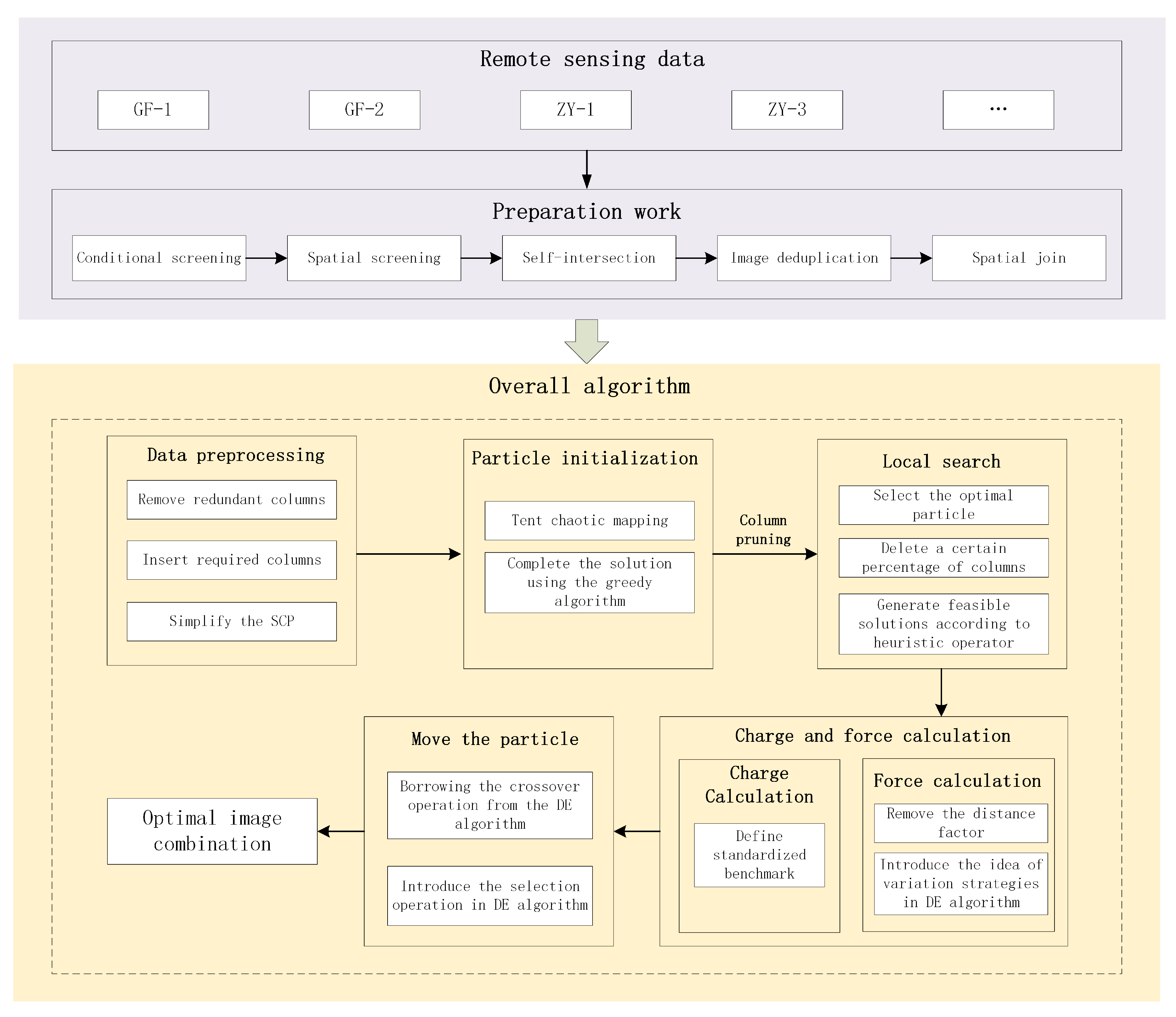
Experiment B: EM algorithm experiment. We use the greedy algorithm to obtain a locally optimal solution and then repeat the local search process m times to generate the initial population. This local search process uses the local search strategy mentioned in Section 2.3.3 of this paper. At this point, after generating a new solution, there may be some redundant columns, so a column pruning process is added. The specific process is to traverse all the columns, if the solution obtained after deleting the column can still cover all the rows, the column is considered to be redundant and the column is deleted.

Experiment C: Tent chaotic map to construct initial population experiment. The method can both fully utilize the traversal advantages of chaos and produce more uniform particles.

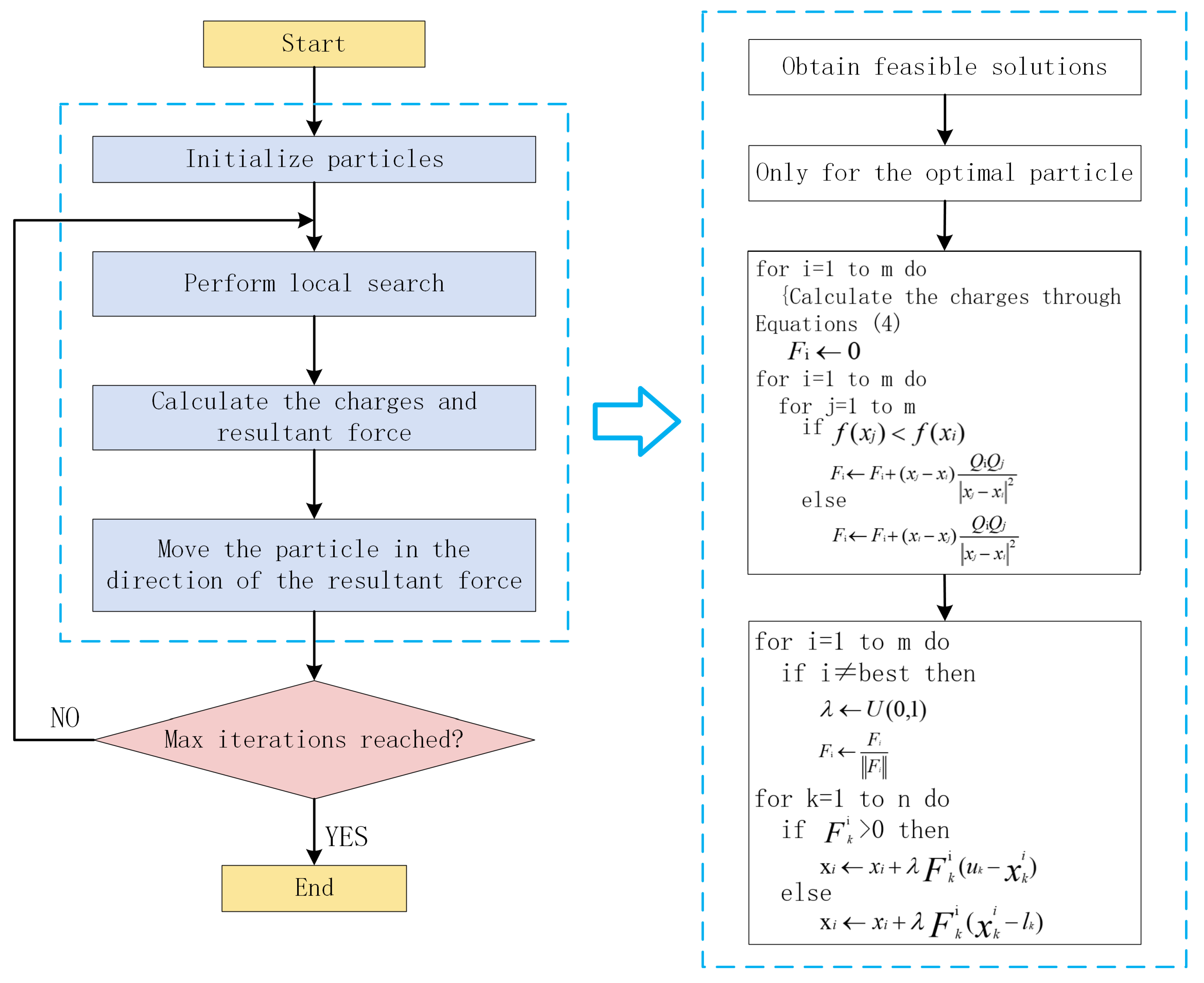
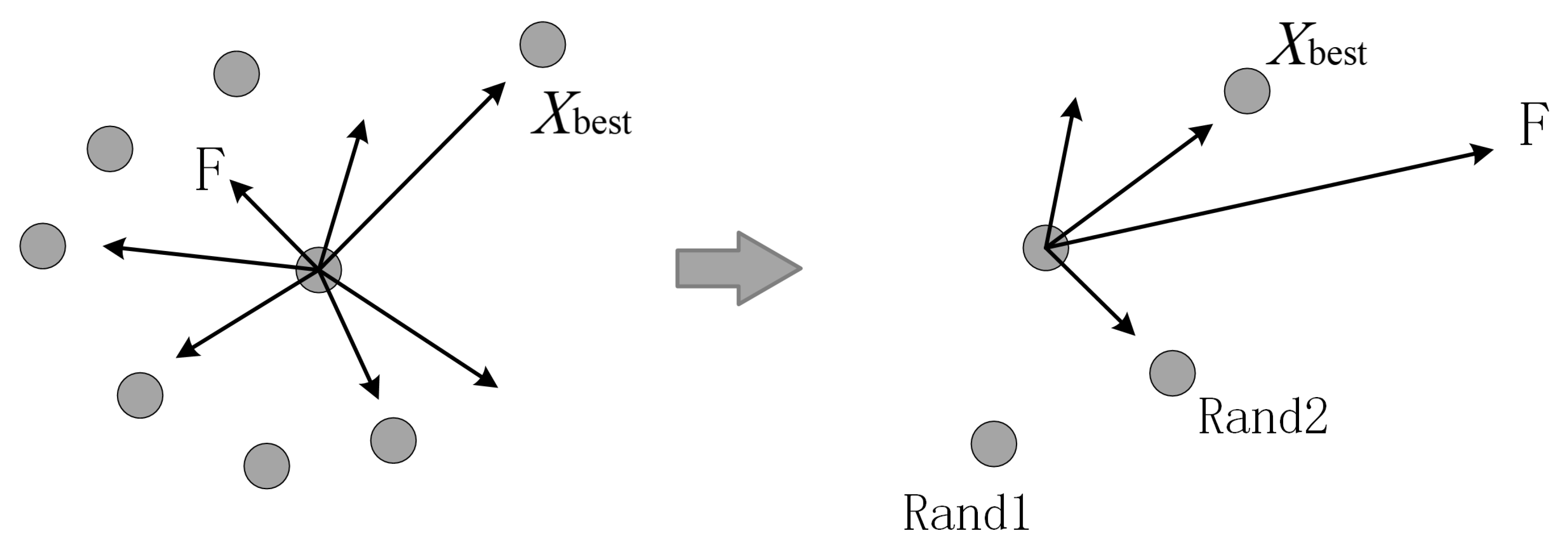
Experiment D: Improved EM algorithm experiment. Based on experiment C, in order to optimize the experimental results and ensure that the particles in the population move towards the optimal solution every time, we introduced the idea of DE algorithm in the process of moving particles.

Experiment E: Comparative Reference Experiment. We respectively use the ant colony optimization algorithm (ACO), the genetic algorithm (GA), and the particle swarm optimization algorithm (PSO) to conduct the optimal screening of remote sensing data for the United States, Hebei 1, Hebei 2, and Inner Mongolia regions, so as to further evaluate the performance and effect of the algorithms in this study.

In experiment BCD, we set the iteration number to 50 and the initial population number to 15 to remain unchanged, and the value range for different deletion column proportion parameters is 0.1–0.5 (0.1, 0.2, 0.3, 0.4, and 0.5). The control parameter pop of different threshold $\alpha$ ranges from 0.7 to 0.95 (0.7, 0.8, 0.85, 0.9, and 0.95).

3.4. Result and Discussion

Based on the U.S. regional datasets, we set the cost of each view image to be the same (i.e., $c_j=1$), resulting in a cost of 1786 for the pre-screening data.

The optimal solution cost of Experiment A is 340, and the result is the same every time. When Experiment C also uses the same column pruning process as Experiment B, the minimum cost is 299, which takes 3497.77 s. From

Table 3. Time proportion of each step in the algorithm (The experimental results of performing the column pruning operation every time a new solution is generated in Experiment C).

Step	Local Search	Charge and Force Calculation	Move the Particle	Column Pruning
Proportion	8.423%	0.093%	10.594%	80.89%

, the column pruning process of Experiment C consumes about 80.89% of the time. After we completely deleted this process, the minimum cost is 315, which takes 1647.24 s. If we only perform column pruning after constructing the initial population, we obtain the minimum cost of 307, which takes 2007.69 s, where the column pruning process consumes 15.38% of the time. From the above experimental results, we can see that column pruning operation is crucial to the optimization of the algorithm. However, considering the influence of time, we choose to carry out the column pruning operation only after generating the initial population, at which time the experimental optimal result is 307, which is reduced by 8–22 compared to Experiment B, and the time consumed is significantly reduced, which is exactly what was adopted for Experiment C recorded in

Table 4. Experimental results (iteration = 50, population = 15; optimal solutions are marked in bold).

Proportion	Pop	EM Algorithm Minimum Cost	Tent Chaotic Map Minimum Cost	Improved EM Algorithm Minimum Cost
0.1	0.7	331	315	301
0.2	0.7	329	315	300
0.3	0.7	329	312	302
0.4	0.7	327	311	303
0.5	0.7	327	309	303
0.1	0.8	332	319	304
0.2	0.8	329	307	303
0.3	0.8	328	310	303
0.4	0.8	326	312	304
0.5	0.8	329	310	304
0.1	0.85	327	317	305
0.2	0.85	325	310	305
0.3	0.85	325	314	301
0.4	0.85	325	311	300
0.5	0.85	325	311	302
0.1	0.9	331	314	303
0.2	0.9	327	307	303
0.3	0.9	330	316	303
0.4	0.9	329	315	305
0.5	0.9	331	310	301
0.1	0.95	329	312	304
0.2	0.95	329	312	301
0.3	0.95	328	312	302
0.4	0.95	327	309	303
0.5	0.95	325	317	304

.

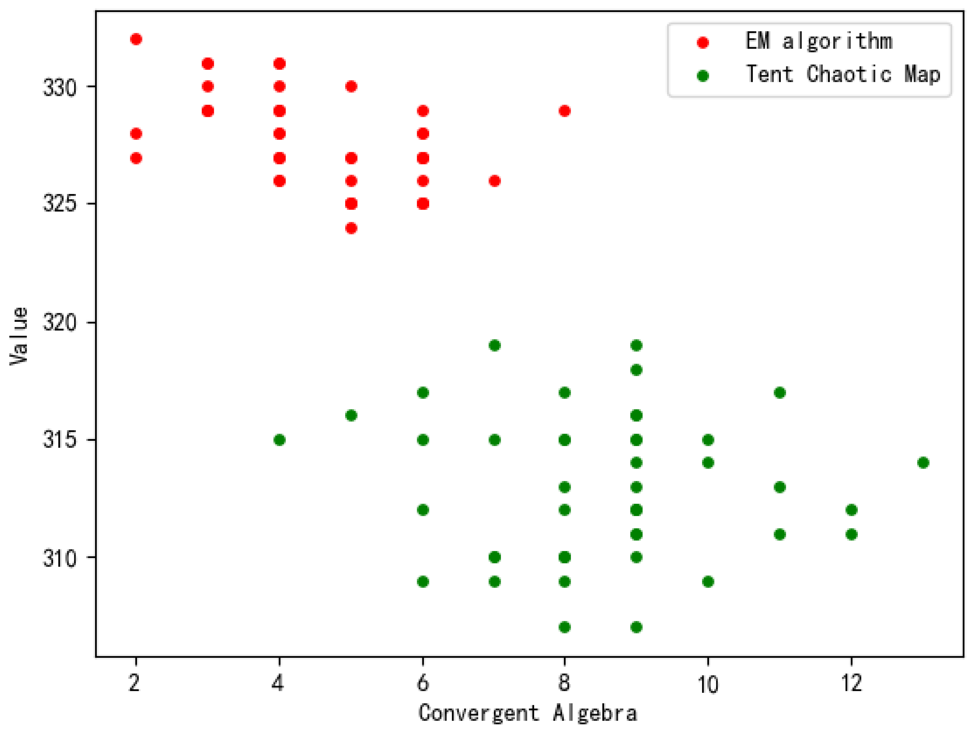
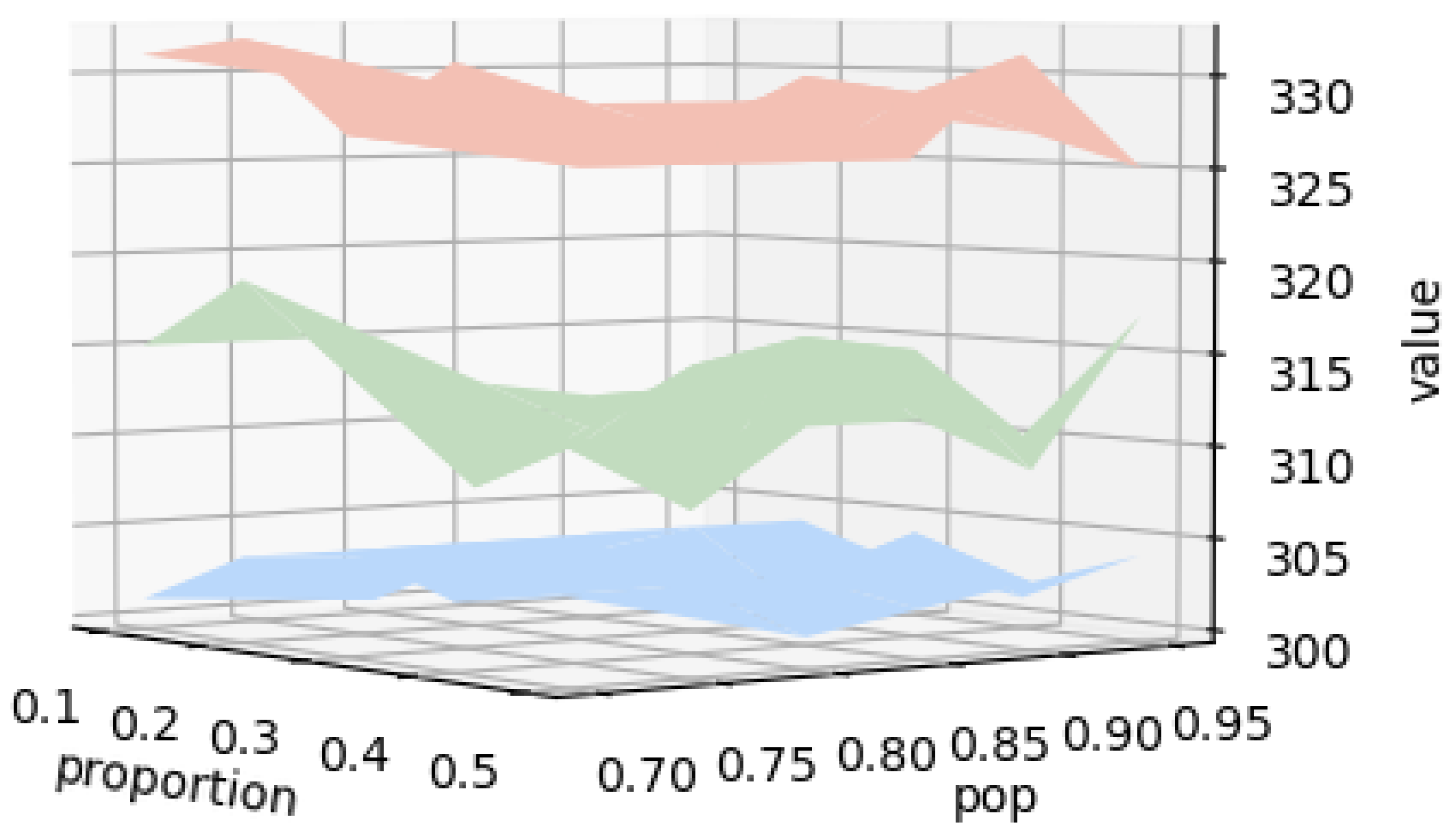
The running results of Experiment BCD are shown in Table 4. We choose the convergence algebra and optimal solution cost in Experiment B and Experiment C to plot the scatter plot. As shown in Figure 5, the initial population constructed by the tent chaotic map has a richer diversity and more uniform distribution, i.e., it is easier to escape from the local optimum, and at the same time, it has a better optimization performance. In Experiment D, we obtain a minimum cost of 300, which takes 1821.54 s. We plotted a 3D surface map based on the different parameter settings of Experiment BCD, with each parameter combination corresponding to a surface, as shown in Figure 6. It can be seen that the experimental results of the improved algorithm are better.

To further explore the effect of population size on the experimental results, we increased the initial population number to 30, and chose the set of parameter configurations that contained the largest number of optimal solutions, i.e., we chose a pop value of 0.85 for the experiment. As shown in

Table 5. Effect of population size on experimental results (iteration = 50).

Proportion	Pop	Minimum Cost (Population = 15)	Minimum Cost (Population = 30)
0.1	0.85	305	301
0.2	0.85	305	300
0.3	0.85	301	298
0.5	0.85	300	301
0.5	0.85	302	299

, when the initial population size is doubled, the minimum cost of 298 is obtained, which takes 4091.61 s. The cost of the optimal solution shows a decreasing trend in general, but the decrease is not significant, while at the same time, the corresponding running time increases significantly. Similarly, in order to determine the effect of the number of iterations on the experimental results, the number of iterations was increased to 100 for the experiments, and it was found that its minimum cost did not fluctuate significantly with the increase in the number of iterations, and its convergence algebra was almost the same as that of 50 iterations in Table 4. After the validation of several repetitions of the experiment, we found that the experiment was able to achieve the optimal balance between efficiency and solution quality when the iteration number is set to 50 and the initial population is set to 15.

Based on the analysis of the above experimental results, we find that the improved EM algorithm proposed in this paper exhibits low sensitivity to these parameter adjustments, which highlights its robustness in the face of parameter changes. In other words, even if the parameters fluctuate within a certain range, the algorithm can still maintain a stable performance. In addition, the implementation of the algorithmic improvement strategy at each step of the process improves the performance of the algorithm, resulting in a more efficient final result compared to the previous one.

In order to verify the feasibility and effectiveness of the improved EM algorithm proposed in this paper to solve the optimization screening problem of remote sensing data, we use the datasets of Hebei and Inner Mongolia for screening. We summarize the results obtained by using other meta-heuristic algorithms for data screening in Experiment E in

Table 6. The results presented by different algorithms when screening different regions.

Region	Raw Data/Scene	Greedy Algorithm Screening Results/Scene	ACO Screening Results/Scene	GA Screening Results/Scene	PSO Screening Results/Scene	Improved EM Algorithm Screening Results/Scene
United States	1786	340	359	346	315	300
Hebei 1	2202	835	841	824	790	775
Hebei 2	511	156	152	151	144	140
Inner Mongolia	2150	685	645	648	628	617

, and through comparative analysis, we find that there are differences in the data screening effects of different algorithms for different regions, which may be related to the characteristics of regional data and the design of the algorithms. In each region, the improved EM algorithm screened the least number of scenes, followed by PSO and greedy algorithm, and the GA and ACO had poor screening results.

Because the greedy algorithm is representative in the field of remote sensing image screening, we use the greedy algorithm as a benchmark method, and we find that the improved EM algorithm improves its optimal solution by about 9.78% on average compared to the greedy algorithm. In order to verify that the improvement was not caused by randomization, we conducted a paired sample t-test and confidence intervals. The original hypothesis (H0) was that there is no significant difference between the screening results of the two methods (mean difference is 0), and the alternative hypothesis (H1) is that there is a significant difference between the screening results of the two methods (mean difference is not 0). The result p-value = 0.0287 < 0.05 was obtained, then, the original hypothesis was rejected and the two methods were considered to show a significant difference in the screening results. Specifically, the mean difference between the two methods is 46, indicating that the greedy screening method is 46 units higher than the improved EM algorithm screening method in terms of screening effectiveness. In addition, the 95% confidence interval ranges from 9.07 to 82.93, which means that we can assume with 95% certainty that the actual mean difference falls within this interval.

These experimental results show that using the improved EM algorithm proposed in this paper to solve the problem can effectively eliminate most of the duplicate coverage data existing in the remote sensing datasets, and obtain the smallest possible dataset that satisfies the conditions, and the optimal solution of the improved EM algorithm is improved by about 9.78% on average compared with the greedy algorithm. Regarding the computational cost, the greedy screening method takes much less time than the improved EM algorithm. Although the improved EM algorithm performs well in screening results, its higher computational cost may limit its application on large-scale datasets. In the future, we will explore optimization strategies to reduce the computational complexity through algorithm optimization and hardware acceleration (e.g., GPU parallel computing). The experimental data in this study are mainly from four regions, and there may be a dependence on region-specific data, which may be affected by the uniformity of regional data distribution. In order to improve the generalization ability of the algorithm, we plan to introduce more diverse datasets in future studies.

The solution of the SCP is not only of theoretical significance, but also has a wide range of applications in real life. For example, by solving the SCP, we can apply its methodology to the fire station location problem [6]. In fire station layout, we need to determine the location of the minimum number of fire stations that can respond quickly to fire and emergency rescue needs throughout the city. This corresponds directly to the goal in the set coverage problem: to select the fewest sets (or regions) such that the concatenation of these sets covers the entire fire risk area of the city. Therefore, the solution of the SCP is not only a theoretical algorithmic optimization, but also an effective tool for solving important problems in real life. As future work, we plan to explore more intelligent optimization algorithms. Additionally, we will actively expand cross-disciplinary applications by integrating deep learning, and apply the results to fields such as urban planning and disaster warning.

3.5. Engineering and Practical Applications

To achieve the efficient screening of massive remote sensing data, we used PyQt5 (The version used in this study is 5.15.9) to encapsulate the code into application software. First, we designed an intuitive graphical user interface (GUI) according to user requirements to enable interaction between users and the algorithm. Subsequently, the developed optimization screening algorithm for remote sensing data was integrated into the PyQt5 framework to ensure the stable operation of the algorithm in the GUI environment. Finally, we used the PyInstaller tool to package the entire project into a standalone.exe file. This process not only simplifies the usage of complex algorithms but also allows non-professionals to operate easily through optimized interaction design. Nowadays, the application has been applied to many practical projects, such as pre-disaster data screening in Pakistan, national land change survey task area data optimization, the optimal selection of basic survey data on water resources, and the national land use dynamics coverage project. Verified by practice, it has significantly shortened the data screening cycle, improved the accuracy and efficiency of data processing, and strongly promoted the development of remote sensing data application.

4. Conclusions

In this paper, we first transform the remote sensing data optimization screening problem into solving the SCP, and secondly, apply the EM algorithm to the SCP, and then, improve the EM algorithm. The improvement idea is as follows:

(1)

Using tent chaotic mapping to construct the initial population so that it can be more uniformly distributed in the feasible domains;

(2)

Combining with a new local search strategy and employ an additional heuristic operator to generate feasible solutions to avoid the algorithm from falling into a local optimum prematurely;

(3)

Normalizing the objective function value to simplify the charge calculation formula, and introducing the idea of variation strategy in differential evolutionary algorithms to simplify the resultant force calculation formula, which significantly reduces the amount of calculation;

(4)

Introducing the idea of differential evolutionary algorithms in moving particle process, which improves the convergence speed of the algorithm.

To verify the effectiveness of the improved EM algorithm proposed in this paper, we utilize the U.S., Hebei, and Inner Mongolia datasets to conduct experiments. The experimental results show that the improved EM algorithm gives better results, searches the global optimal solution faster, and has better robustness. Taking the dataset discussed in this paper as an example, compared with the greedy algorithm, the optimal solution obtained in this study has been improved by 9.78% on average. This achievement has been successfully applied to data optimization scenarios in practical work with remarkable effectiveness, which not only effectively reduces the cost of data storage, transmission, and processing, but also practically improves the work efficiency. Moreover, it strongly supports the data services of various remote sensing applications such as urban and rural planning [24], natural disaster and environmental monitoring [25], and land resource surveys [26], thereby enhancing the utilization efficiency and application value of data.

References

1. Yan, X.; Liu, W.; Liu, S.; Duan, J.; Xia, W. Screening method of remote sensing image region covering dataset. J. Univ. Chin. Acad. Sci. 2023, 40, 523–530. [Google Scholar] [CrossRef]
2. Zhu, L.; Su, X.; Hu, Y.; Tai, X.; Fu, K. A Spatio-Temporal Local Association Query Algorithm for Multi-Source Remote Sensing Big Data. Remote Sens. 2021, 13, 2333. [Google Scholar] [CrossRef]
3. He, F. Research on Massive Remote Sensing Data Retrieval Techniques Based on Spatial Grid Filtering. Master’s Thesis, Henan University, Kaifeng, China, 2017. [Google Scholar]
4. Yang, X.; Yan, J. Research on Optimal Region Covering Algorithm for ZY-3 Satellite Image. J. Geomat. 2019, 44, 71–74. [Google Scholar] [CrossRef]
5. Ge, H.; Gao, Y. Ant colony algorithm for solving set-covering problems. Comput. Eng. Appl. 2007, 43, 49–50. [Google Scholar] [CrossRef]
6. Soto, R.; Crawford, B.; Olivares, R.; Barraza, J.; Figueroa, I.; Johnson, F.; Paredes, F.; Olguín, E. Solving the non-unicost set covering problem by using cuckoo search and black hole optimization. Nat. Comput. 2017, 16, 213–229. [Google Scholar] [CrossRef]
7. Luo, L.; Li, Q. Research on location of emergency logistics facilities based on improved ensemble coverage model. Technol. Mark. 2021, 28, 9–11. [Google Scholar]
8. Song, J.; Mao, Y.; Ai, Y.; Shen, J.; Zou, Y. Research on optimization for community cainiao Station Site Selection Based on Set Coverage Model. Mod. Inf. Technol. 2023, 7, 8–13. [Google Scholar] [CrossRef]
9. Li, X.; Qin, H.; Wang, Y.; Zhao, S.; Yang, J.; Yang, L. Research on Location Problem Based on Set Coverage Model and Linear Weighted Sum Method—Taking the Site Selection of Emergency Logistics Center in Lanzhou Heping University Cluster as an Example. Logist. Sci.-Tech. 2024, 47, 9–12. [Google Scholar] [CrossRef]
10. Tian, Y.; Liu, A.; Yan, J.; Fan, J. Research on energy saving technology of base station based on collective coverage in cellular network. Electron. Des. Eng. 2022, 30, 156–159. [Google Scholar] [CrossRef]
11. Naji-Azimi, Z.; Toth, P.; Galli, L. An electromagnetism metaheuristic for the unicost set covering problem. Eur. J. Oper. Res. 2010, 205, 290–300. [Google Scholar] [CrossRef]
12. Dorigo, M.; Maniezzo, V.; Colorni, A. Ant system: Optimization by a colony of cooperating agents. IEEE Trans. Syst. Man Cybern. Part B Cybern. 1996, 26, 29–41. [Google Scholar] [CrossRef]
13. Caserta, M. Tabu Search-Based Metaheuristic Algorithm for Large-scale Set Covering Problems. Metaheuristics Prog. Complex Syst. Optim. 2007, 39, 43–63. [Google Scholar] [CrossRef]
14. Brusco, M.J.; Jacobs, L.W.; Thompson, G.M. A morphing procedure to supplement a simulated annealing heuristic for cost- and coverage-correlated set-covering problems. Ann. Oper. Res. 1999, 86, 611. [Google Scholar] [CrossRef]
15. Al-Sultan, K.S.; Hussain, M.F.; Nizami, J.S. A Genetic Algorithm for the Set Covering Problem. J. Oper. Res. Soc. 1996, 47, 702–709. [Google Scholar] [CrossRef]
16. Crawford, B.; Soto, R.; Olivares-Suarez, M.; Paredes, F.; Johnson, F. A Binary Firefly Algorithm for the Set Covering Problem. Mod. Trends Tech. Comput. Sci. 2014, 285, 65–73. [Google Scholar] [CrossRef]
17. Crawford, B.; Soto, R.; Berrios, N.; Johnson, F.; Paredes, F.; Castro, C.; Norero, E. A Binary Cat Swarm Optimization Algorithm for the Non-Unicost Set Covering Problem. Math. Probl. Eng. 2015, 2015, 578541. [Google Scholar] [CrossRef]
18. Crawford, B.; Soto, R.; Pena, C.; Riquelme-Leiva, M.; Torres-Rojas, C.; Johnson, F.; Paredes, F. Binarization Methods for Shuffled Frog Leaping Algorithms That Solve Set Covering Problems. Softw. Eng. Intell. Syst. 2015, 349, 317–326. [Google Scholar] [CrossRef]
19. Crawford, B.; Soto, R.; Pena, C.; Palma, W.; Johnson, F.; Paredes, F. Solving the Set Covering Problem with a Shuffled Frog Leaping Algorithm. Intell. Inf. Database Syst. 2015, 9012, 41–50. [Google Scholar] [CrossRef]
20. Birbil, S.I.; Fang, S.C. An electromagnetism-like mechanism for global optimization. J. Glob. Optim. 2003, 25, 263–282. [Google Scholar] [CrossRef]
21. Wang, S. The Improvement and Application of Electromagnetism-Like Mechanism Algorithm. Master’s Thesis, Xidian University, Xi’an, China, 2012. [Google Scholar]
22. Wang, L. Research on Batch Coordinate Transformation Method Based on ArcGIS. Geomat. Spat. Inf. Technol. 2021, 44, 132–134. [Google Scholar] [CrossRef]
23. Zhang, X.; Wei, S. Improved Equilibrium Optimizer Algorithm Based on Tent Chaotic Map and Random Walk Strategy. J. Taiyuan Norm. Univ. Nat. Sci. Ed. 2024, 23, 6–9. [Google Scholar]
24. He, T.; Wang, S. Application of Remote Sensing Technology in Urban and Rural Planning and Construction Inspectors—Monitoring the Status of Urban Land Use. Image Technol. 2012, 24, 52–56. [Google Scholar] [CrossRef]
25. Dou, C.; Li, Z. A Brief Discussion on the Development and Application of Photogrammetry and Remote Sensing. Manag. Strategy Qinghai Land Resour. 2011, 6, 29–31. [Google Scholar] [CrossRef]
26. Zhang, D. Current status and development trend of remote sensing technology application for land resources. Agric. Technol. 2018, 38, 253. [Google Scholar]
Figure 1. Technology roadmap.
Applsci 15 03542 g001
Figure 2. Flowchart of EM algorithm.
Applsci 15 03542 g002
Figure 3. Diagram of the improved resultant force calculation process. The original algorithm’s calculation of the current particle’s resultant force requires the calculation of the resultant force of all other particles on its component forces, whereas the improved algorithm selects only the optimal particle X b e s t as well as two randomly selected particles from the remaining particles to perform the calculation.
Applsci 15 03542 g003
Figure 4. Examples of Gaofen-1 and Gaofen-2 images. (a) Gaofen-1 image. (b) Gaofen-2 image.
Applsci 15 03542 g004
Figure 5. Experimental results of initial population construction using EM algorithm and tent chaotic map.
Applsci 15 03542 g005
Figure 6. Experiment with 3D surface map (corresponding to Experiment BCD from top to bottom).
Applsci 15 03542 g006