Abstract
This study aims to improve the prediction accuracy of reference evapotranspiration under limited meteorological factors. Based on the commonly recommended PSO-ELM model for ET0 prediction and addressing its limitations, an improved QPSO algorithm and multiple kernel functions are introduced. Additionally, a novel evapotranspiration prediction model, Kmeans-QPSO-MKELM, is proposed, incorporating K-means clustering to estimate the daily evapotranspiration in Yancheng, Jiangsu Province, China. In the input selection process, based on the variance and correlation coefficients of various meteorological factors, eight input models are proposed, attempting to incorporate the sine and cosine values of the date. The new model is then subjected to ablation and comparison experiments. Ablation experiment results show that introducing K-means clustering improves the model’s running speed, while the improved QPSO algorithm and the introduction of multiple kernel functions enhance the model’s accuracy. The improvement brought by introducing multiple kernel functions was especially significant when wind speed was included. Comparison experiment results indicate that the new model’s prediction accuracy is significantly higher than all other comparison models, especially after including date sine and cosine values in the input. The new model’s running speed is only slower than the RF model. Therefore, the Kmeans-QPSO-MKELM model, using date sine and cosine values as inputs, provides a fast and accurate new approach for predicting evapotranspiration.
1. Introduction
With the growth of the global population, the shortage of freshwater resources is becoming increasingly severe. However, worldwide, agriculture accounts for 70% of total water usage; of that, approximately 60% is lost through evaporation. The prediction of evapotranspiration (ET0) is crucial for calculating agricultural irrigation requirements, as well as for the design, optimization, and management of irrigation systems and water resources [1,2,3,4]. The widely recognized standard for calculating ET0 is the FAO-56 Penman–Monteith equation [5], proposed by the Food and Agriculture Organization (FAO), which has been extensively used for calculating reference evapotranspiration (ET0) values [6,7,8,9]. However, the FAO-56 Penman–Monteith equation requires numerous meteorological variables, many of which are often incomplete or missing, particularly in developing countries. This limitation restricts the direct application of FAO-56 [10,11]. As a result, researchers have developed and calibrated various simplified models and empirical formulas for estimating evapotranspiration, such as the Makkink, Priestley–Taylor, and Hargreaves models. However, evaluations in practical applications have shown that these models often exhibit significant deviations in prediction accuracy [12,13,14], and many coefficients require region-specific adjustments [15]. Therefore, there is a need to identify methods that can more accurately predict ET0 under conditions with limited meteorological data.
In recent years, with the rapid development of machine learning, it has been widely applied to predicting evapotranspiration. Many common machine learning algorithms, such as Artificial Neural Network (ANN) [16], Random Forest (RF) [6,17], Support Vector Machine (SVM) [17,18,19], Adaptive Neuro-Fuzzy Inference Systems (ANFIS) [16,18], Multivariate Adaptive Regression Splines (MARS) [18], and M5P [17], have been used to model and predict ET0, yielding promising results. Among these, the Extreme Learning Machine (ELM) model has garnered significant attention in academia and industry due to its fast and efficient computation, excellent generalization ability, and strong adaptability [20]. Abdullah et al. (2015) were the first to apply the ELM model to predict evapotranspiration. They used the ELM model and the Feedforward Backpropagation Neural Network (FFBP) to predict ET0 at three sites across Iraq. Their study found that the ELM model exhibited excellent predictive capability for daily ET0 outperformed the FFBP model in prediction accuracy and efficiency, even when incomplete meteorological data were used. They strongly recommended the ELM model for evapotranspiration prediction [21].
Since then, many researchers have attempted to use the ELM model to predict evapotranspiration in different regions and under various input conditions, all finding that it delivers superior performance in ET0 prediction. For example, Kumar et al. (2016) used ELM, ANN, Genetic Programming (GP), and SVM to model and predict ET0 for Pusa in Bihar, India. They found that ELM achieved significantly higher prediction accuracy than the other three models with much shorter computation times [22]. Similarly, Fan et al. (2018) used SVM, ELM, and four tree-based ensemble models to model and predict daily evapotranspiration for different climatic regions in China. Their results showed that SVM and ELM had higher prediction accuracy and stability than the other models, with the ELM model slightly outperforming the SVM model [17].
In machine learning, a model’s performance is closely related to the setting of its parameters. Optimization algorithms can continuously refine the parameters by searching for the optimal solution, significantly improving the predictive accuracy of machine learning models. Therefore, optimization algorithms are widely used in conjunction with machine learning models, and their advantages are continuously validated in practice [23,24,25]. The ELM model does not require iterations compared to other machine learning models. The connection weights between the input layer and the hidden layer, as well as the thresholds of the hidden layer, are randomly generated, which gives ELM a breakneck computational speed. However, this also means that ELM may not consistently achieve optimal performance and leaves room for further optimization. As a result, many optimization algorithms have been applied to enhance ELM. In the field of evapotranspiration prediction, Particle Swarm Optimization (PSO) has been repeatedly shown to be one of the most effective methods for optimizing ELM, making it a popular and widely used model in evapotranspiration prediction.
For example, Zhu et al. (2020) optimized the ELM model using PSO for evapotranspiration modeling and prediction in northwestern China’s temperate continental climate region. They compared the performance of the PSO-ELM model with the original ELM, ANN, RF, and six empirical models regarding prediction accuracy. The results indicated that PSO enhanced the performance of ELM, outperforming other machine learning and empirical models [12]. Similarly, Wu et al. (2021) used Genetic Algorithm (GA), PSO, and Artificial Bee Colony (ABC) algorithms to optimize ELM for ET0 prediction at 12 representative stations across five different climatic regions in China. Their results showed that all optimization algorithms significantly improved the prediction accuracy of ELM, with the PSO-ELM model performing the best [13]. Additionally, Shi et al. (2023) optimized the ELM model using GA, PSO, and Salp Swarm Algorithm (SSA) to predict ET0 at 23 stations in China. Their findings demonstrated that the PSO-ELM model had the highest prediction accuracy and most excellent applicability [26]. These studies highlight the significant performance improvements achieved by using PSO to optimize ELM for ET0 prediction, establishing PSO-ELM as a practical and superior approach.
However, the traditional PSO algorithm has some drawbacks, such as the tendency to get stuck in local optima in complex multimodal problems, the lack of randomness in particle position updates, and the rapid decrease in population diversity as iterations progress, which negatively impacts its global search capability. To address these limitations, the Quantum Particle Swarm Optimization (QPSO) algorithm, which incorporates quantum theory, has been proposed to enhance the diversity of the population, improve global search ability, and balance global and local searches, thus reducing the likelihood of getting trapped in local optima [27]. QPSO has been applied in many fields and has improved performance [28,29,30]. In recent years, the improved Kernel Extreme Learning Machine (KELM) model has been proposed. It introduces a kernel function into the ELM model, which maps the data to a higher-dimensional space, thereby enhancing the ELM model’s ability to handle nonlinear data. Since the factors involved in evapotranspiration (ET0) prediction are complexly interrelated and highly nonlinear, this approach has also been applied to ET0 prediction and has yielded promising results [31,32]. However, using a single kernel function limits its adaptability to handle complex and diverse data types. To overcome this, multi-kernel functions can be introduced, which, by optimizing the weightings of different kernels, further enhance the model’s ability and adaptability to handle data with different features [33,34,35,36].
In the KELM model, computing the kernel matrix becomes very time-consuming when the sample size is large. By applying clustering algorithms to group-related samples and building models for each group, the computational load of the kernel matrix can be significantly reduced, resulting in lower computational costs [32]. Therefore, the main objectives of this study are as follows: (1) To propose an improved QPSO-MKELM model based on the PSO-ELM model, then introduce the K-means-QPSO-MKELM model. The model’s prediction accuracy and computation time will be compared for different numbers of clusters to determine the optimal number of clusters. (2) To conduct ablation experiments on the proposed K-means-QPSO-MKELM model. (3) To compare the prediction accuracy and computation time of K-means-QPSO-MKELM, QPSO-MKELM, PSO-ELM, RF, Whale Optimization Algorithm–Support Vector Regression (WOA-SVR), and ANFIS.
2. Materials and Methods
2.1. Study Area and Data Information
The study area is located in Yancheng, China, within the Huaihe River Basin, at a latitude of 32.75° and a longitude of 120.25°, with an elevation of 3 m. Yancheng is home to the Dafeng Farm, one of China’s significant agricultural regions. The dataset includes temperature, humidity, wind speed, sunshine duration, and precipitation. It was obtained from the China Meteorological Data Service Center and has undergone strict manual review and rigorous quality control, ensuring high reliability with no prolonged missing periods. No extreme outliers were detected upon inspection, and the missing data rate was 0.26%. Missing values were imputed using linear interpolation. The dataset consists of daily meteorological data from 1980 to 2023, spanning 44 years. Among these, data from 1980 to 2018 (39 years) were used for training the model, while data from 2019 to 2023 (5 years) were used for testing the model.
2.2. FAO-56 Penman–Monteith Model
The FAO-56 model, proposed by Allen et al. (1998), is a formula-based model for calculating evapotranspiration [5] and is known for its high computational accuracy. Since no experimental ET0 data are available in the study area, FAO-56 was used to calculate ET0 as the reference target output for machine learning models. This approach is acceptable and commonly employed under such circumstances [37]. The specific formula is as follows:
where ET0 (mm/d) is the reference evapotranspiration, Rn (MJ/m2/d) is the net radiation, G (MJ/m2/d) is the soil heat flux density, Tmeans (°C) is the mean air temperature, ea (kPa) is the actual vapor pressure, es(kPa) is the saturated vapor pressure, Δ is the slope of the vapor pressure curve, γ is the psychrometric constant, and U2 (m/s) is the wind speed at 2 m above the ground. Allen et al. (1998) provides the detailed calculation process of this model [5]. Additionally, radiation is calculated from sunshine duration using the Angström equation [38].
2.3. Correlation Analysis and Variance
Evapotranspiration (ET0) has a complex nonlinear relationship with various meteorological factors, and among these, the FAO-56 model, while highly accurate, requires many meteorological inputs. However, these inputs are often incomplete, which limits the model’s applicability. In contrast, machine learning can build models and make predictions even when data are incomplete. It is important to note that different meteorological data contain varying amounts of information about evapotranspiration. Thus, we can perform correlation and variance analyses to preliminarily select features, providing a valuable reference for constructing the final model.
Correlation analysis is used to study the relationships between variables or between variables and outputs. This study employs the maximal information coefficient (MIC) [39], a correlation measure from information theory. MIC can capture both linear relationships between features and evapotranspiration, as well as complex nonlinear relationships among them.
Variance is a statistical measure that describes the degree of data dispersion and quantifies how much data points deviate from the mean. The variance of a feature reflects its numerical variation range. However, variances cannot be directly used to measure information content due to differences in units and scales among features. By computing the variance of normalized features, the variation of different features can be compared on the same scale, enabling the quantification of the information contained in each feature; the larger the normalized variance, the more information the feature carries.
2.4. New Model
2.4.1. K-Means Clustering
K-means is a widely used and simple clustering algorithm. It divides the dataset into k clusters, aiming to minimize the distance between data points within each cluster so that data points in the same cluster are more similar to each other than to points in different clusters.
Its principle and steps are as follows: first, the number of clusters k is set. Then, k data points are randomly selected as centroids. The data points are assigned to the nearest centroid’s cluster by calculating the Euclidean distance. The mean of the data points within each cluster is then recalculated to serve as the new centroid. The process of reassigning points to clusters and recalculating centroids is repeated until the change in centroids is below a set threshold, at which point the iteration stops. Once the iteration ends, all data points are assigned to one of the k clusters, completing the clustering process.
The K-means clustering algorithm operates in the original feature space, and its calculation is straightforward and efficient. It is suitable for large datasets and can perform clustering with relatively low computational cost. However, it also has some drawbacks. The value of k must be set in advance, and in practical applications, this value can be challenging to determine. Accurately setting k requires a good understanding of the dataset. In real-world applications, the value of k is usually determined by trying different values and comparing the clustering results.
2.4.2. MKELM
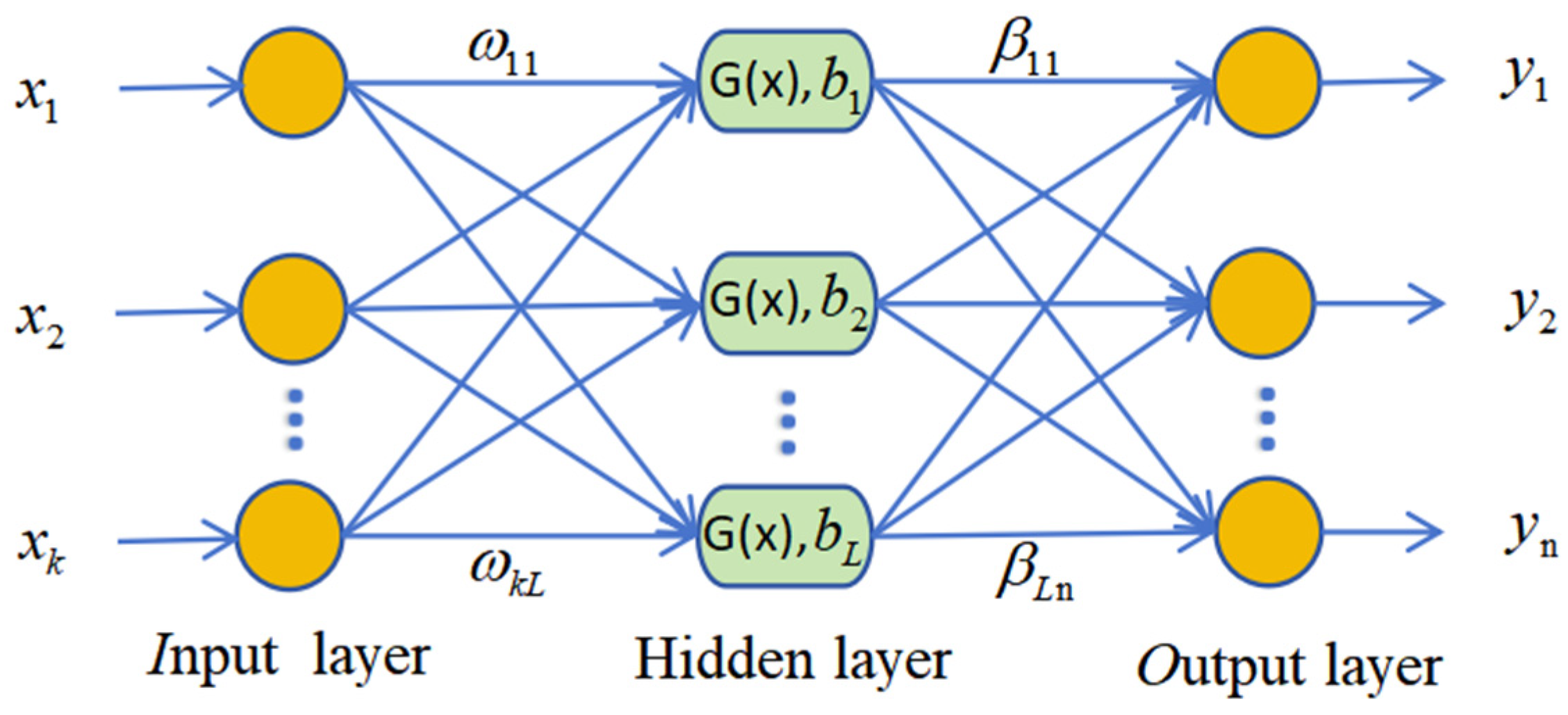
The ELM [40] is a single hidden-layer neural network proposed by Huang, GB, in 2006. As shown in Figure 1, its network structure consists of the input layer, hidden layer, and output layer. Compared to traditional BP neural networks and support vector machines, the weights between the hidden layer and the output layer are determined by solving the generalized inverse matrix. This eliminates the need to adjust connection weights, resulting in breakneck computation speed.
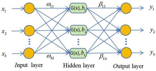
Figure 1.
Structure diagram of Extreme Learning Machine.
Let x1 to xk represent the k-dimensional input of the sample and y1 to yn represent the n-dimensional target output. An ELM with L hidden layer neurons can be expressed as:
Let X be the input matrix and ω be the connection weights randomly generated between the input nodes and the hidden layer nodes. bi represents the bias of the i-th hidden layer node. G(x) is the activation function of the hidden layer.
The equation can be expressed as:
where H is the feature mapping from the k-dimensional input space to the L-dimensional space, representing the hidden layer’s output matrix, and is the weight vector from the hidden layer to the output layer. By applying regularized least squares to minimize the loss function, the solution is obtained:
The least squares solution can easily lead to overfitting, which limits the model’s generalization ability. Therefore, a regularization parameter C is introduced to reduce the risk of overfitting.
The output weights are then obtained as:
Kernel functions are introduced to enhance the performance of the ELM, leading to the KELM algorithm [41]. The main difference between KELM and ELM is that the kernel function, through kernel mapping, increases the dimensionality of the data, mapping linearly non-separable data in a low-dimensional space to a higher-dimensional space where it becomes linearly separable.
The kernel matrix can be defined as:
The kernel matrix based on the kernel function replaces the HHT, h(x) is the output matrix of the hidden layer, and K(xi,xj) represents the kernel function. The output of the KELM can be expressed as:
Random mapping is replaced with kernel mapping, which eliminates the need to set the number of hidden layer nodes during the initialization phase. Additionally, there is no need to set the hidden layer node weights and thresholds, effectively improving the generalization ability and stability that could be compromised by random initialization of hidden layer weights.
The KELM introduces kernel functions, enhancing the ELM performance when dealing with nonlinear problems. However, the kernel function in KELM is a single, static function, which limits its ability to handle complex data structures and its adaptability to different data types and features [33,34,35,36]. Therefore, this paper introduces multiple kernel functions, which are combined linearly to form a final kernel function. The weight of each kernel function is optimized through an algorithm. This enables the model to adapt to data characteristics from multiple dimensions and perspectives, improving the model’s learning and generalization abilities. As a result, the model demonstrates more stable performance across various scenarios.
This study selects the following kernel functions to construct the multiple kernel function: RBF (Radial Basis Function) kernel, linear kernel, and polynomial kernel. The linear kernel can capture the linearly separable parts of the data well without increasing the model’s complexity. The RBF kernel maps the data into an infinite-dimensional space, effectively handling linearly non-separable data structures in the original space. The polynomial kernel is capable of handling high-dimensional polynomial structures in the data. These kernels are combined, and their weights are optimized.
The parameters that need to be optimized in the MKELM include the width of the Gaussian kernel (σ), the degree of the polynomial kernel (d), the regularization parameter C, and the weights of the three kernel functions, namely c1, c2, and c3, where c1 + c2 + c3 = 1.
2.4.3. Piecewise QPSO Improved by GA
The traditional PSO algorithm updates the velocity and position of the particles in the next generation based on the particle’s velocity inertia, individual best, and global best, which carries a significant risk of getting stuck in local optima. To address this issue, Jun Sun et al. introduced quantum theory into the Particle Swarm Optimization algorithm, resulting in the QPSO algorithm [27]. In the QPSO algorithm, the particle’s position update formula is as follows:
where is the local attraction point for the i-th particle, and its formula is as follows:
Pi (t) is the individual best position of the i-th particle at the t-th iteration, and Pg(t) is the global best position at the t-th iteration.
(t) is the shrinkage-expansion coefficient; Nbest(t) is the average position of all particles’ individual best positions at the t-th iteration; and are random numbers uniformly generated within the range [0, 1]. The formula for calculating Nbest(t) is as follows:
The formula for calculating (t) is as follows:
where t is the current iteration number, and T is the maximum number of iterations. The local attraction point, , is important in the particle position update. It is a linear combination of the individual and global best positions. is a random number in the range [0, 1]. Although the particle can integrate individual and population information to update its position, the search lacks emphasis on different stages. This paper proposes a piecewise attraction point, which adjusts the emphasis on the dominance of individual and global best in different stages. The parameter is bounded by a maximum value of instead of 1. When exceeds 0.5, is a random number in the range [0.5, ]. Otherwise, it is in the range [0, ]. The formula for is as follows:
At the early stages of the algorithm, has a higher probability of selecting larger values, and the individual best dominates in the attraction point, improving the particle’s global search ability and avoiding premature convergence to local optima. In the later stages, the probability of selecting smaller values for increases, and the global best dominates in the attraction point.
The improvement of the piecewise attraction point enhances the global search ability of the particle. However, there is still a possibility of getting stuck in local optima during the particle convergence phase. To address this, the idea of genetic algorithm mutation is introduced. A piecewise mutation strategy is proposed. A minimal mutation probability is applied in the early stages when the particles are still relatively dispersed. This ensures that the search and convergence of the particles are not affected. In the later stages, when the particles converge to a certain extent, and the population becomes highly similar, the mutation rate increases. At this point, increasing the mutation rate has little effect on the convergence trend of the population but greatly improves the ability of the population to escape from local optima, further enhancing the model’s global search ability and stability, and reducing the risk of the model getting trapped in local optima. The mutation rate λ is calculated as follows:
where λ is a random number in the range of [0, 0.1], when < 0.09; otherwise, λ is a random number in the range of [0.09, ].
2.4.4. QPSO-MKELM Model and Kmeans-QPSO-MKELM Model
The QPSO-MKELM model is constructed by optimizing the hyperparameters of the MKELM using a Segmented QPSO improved by GA. These hyperparameters include the Gaussian kernel width (σ), polynomial kernel degree (d), regularization parameter C, and the weight parameters of the three kernel functions (c1,c2,c3).
The Kmeans-QPSO-MKELM model first divides the training set into k clusters using K-means clustering. The k clusters are then treated as k subsets of the original dataset. For each k subset, a QPSO-MKELM sub-model is trained, and all k sub-models are combined to form the final model. In this study, the Kmeans-QPSO-MKELM model adopts a weighted scheme during the testing phase. First, the Euclidean distance between each data point in the test set and the centroids of the k clusters is calculated. The two clusters whose centroids are closest to the test point are selected, and the corresponding sub-models are used to make predictions. The final prediction is then computed using a weighted averaging approach, where the weights are determined by the formula 1/(d^6). In this study, k was chosen as 10, 20, 30, and 40 for comparative experiments.
2.5. Hardware and Software Configuration & Program Execution Time
The machine learning models in this experiment were run on a computer with an Intel Core i5-1135G7 CPU, Intel Iris Xe Graphics GPU, and 16 GB RAM, using MATLAB R2023b software.
The model execution time reported in this study refers to the training time of the models, which is the average time taken from running each model five times.
2.6. Performance Comparison Criteria
This study uses R2, MAE, RMSE, and (Global Performance Index) Gp [26,42,43,44] as evaluation metrics to assess the performance of different models. The specific calculation methods and formulas for R2, MAE, and RMSE can be found in reference [45]. The specific calculation formula for Gp [26] is as follows:
where Tj is the normalized value of the three evaluation metrics (R2, MAE, RMSE), and Mj is the median value of the corresponding evaluation metric. When Tj corresponds to R2, αj is 1; for other cases, αj is −1.
The higher the R2 value, the better the model’s fit to the data, indicating better performance. The lower the RMSE and MAE, the better the model’s performance. The higher the Gp value, the better the overall performance of the model. Gp-Rank ranks the models based on their Gp values, from the highest to the lowest.
3. Results and Analysis
3.1. Model Input Selection
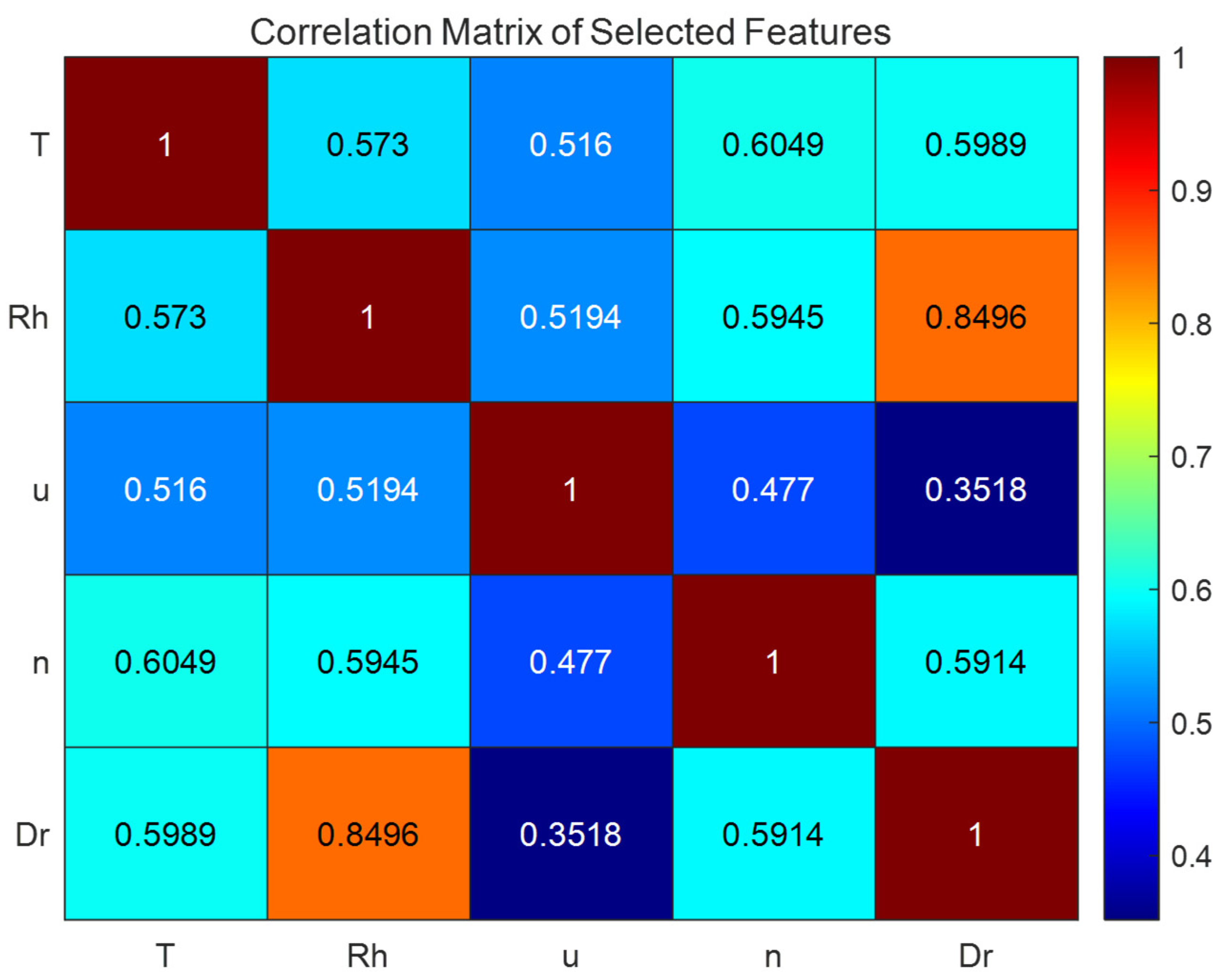
Table 1 provides the basic statistical summary of meteorological factors in the dataset for the study area. First, the average temperature (T), humidity (Rh), 2 m average wind speed (u), sunshine duration (n), daily precipitation (Dr), and ET0 were normalized. Then, the variance between each input meteorological factor was calculated (Table 2), and the correlation with ET0 was calculated (Table 3). Next, the correlation between each input meteorological factor was calculated (Figure 2). Finally, the monthly average of the daily ET0 in the study area was plotted (Figure 3).

Table 1.
Basic statistical summary of meteorological factors in the dataset for the study area.
Table 2.
Variance of each input meteorological factor after normalization.
Table 3.
Correlation coefficient between each meteorological factor and ET0.
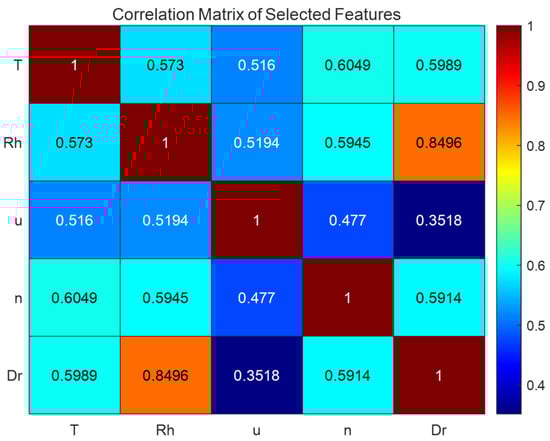
Figure 2.
Correlation heatmap between each input meteorological factor.
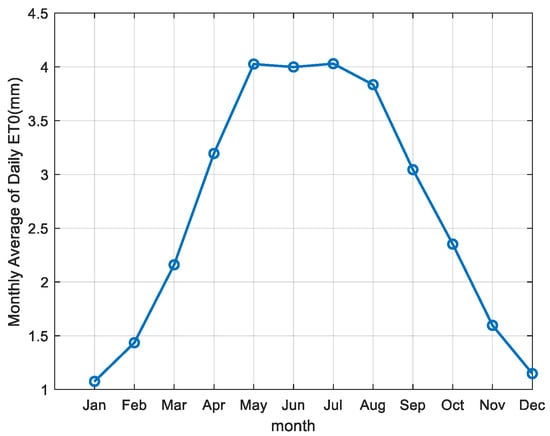
Figure 3.
Monthly average of daily evapotranspiration over 44 years in the study area.
The correlation coefficients of temperature and sunshine duration with ET0 reached as high as 0.8660 and 0.9298 (Table 3), which are highly correlated and much higher than the other features. Their normalized variances are 0.0454 and 0.0551 (Table 2), respectively, which are also the highest among all features. Therefore, they are initially considered to contain the most information about ET0 and are the two most important meteorological factors for predicting daily ET0. The correlation coefficients of humidity, wind speed, and precipitation with ET0 are 0.5895, 0.5705, and 0.5536 (Table 3), respectively, relatively close. Their normalized variances are 0.0268, 0.015, and 0.0035 (Table 2). The variance of the humidity feature is greater than that of wind speed and much larger than that of precipitation. If the correlation between features is not considered, humidity and wind speed would be the third and fourth most important features. The heatmap of feature correlations shows that the correlation coefficient between humidity and precipitation is as high as 0.8496 (Figure 2), the only feature pair with a correlation coefficient above 0.8, indicating a strong correlation and significant information redundancy. Therefore, precipitation was excluded from the input. It is concluded that humidity and wind speed are the third and fourth most important factors for predicting evapotranspiration in the current region, although their importance is far less than that of temperature and sunshine duration.
Evapotranspiration exhibits a uniform variation trend throughout the year [46,47], and this is also true for the region in this study. As shown in Figure 3, evapotranspiration in the study area changes uniformly and shows strong periodicity. Moreover, the day of the year can be converted directly without additional sensor measurements.Therefore, the day of the year was also considered as an input to observe its impact on the machine learning model’s prediction accuracy. Since the day of the year is periodic, the last day of the year and the first day of the following year are theoretically closest, yet numerically, they are farthest apart. To address this, trigonometric functions, sin(day) and cos(day), were used to transform the day of the year for input.
Based on this, the study proposed and developed eight input models for evaluation (Table 4).
Table 4.
Correspondence between input models and features.
3.2. Performance of QPSO-MKELM and Kmeans-QPSO-MKELM with Different Numbers of Clusters
In this study, the QPSO-MKELM model was established for each of the eight input models proposed earlier. Additionally, Kmeans-QPSO-MKELM models were built with k values of 10, 20, 30, and 40 for the K-means algorithm. The prediction accuracy and training time for each model were recorded, and the results are shown in Table 5 and Figure 4.
Table 5.
Error metrics and runtime statistics of QPSO-MKELM and Kmeans-QPSO-MKELM Models.
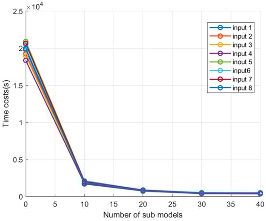
Figure 4.
Comparison of program runtime for each model under different inputs.
From Figure 4 and Table 5, it can be seen that for models with the same number of clusters, the training time trends under different feature inputs are generally similar. The training time for the QPSO-MKELM model under different feature inputs ranged from 18,364 s to 20,933 s, significantly higher than the training time of other models. The average training times for the Kmeans-QPSO-MKELM-10, Kmeans-QPSO-MKELM-20, Kmeans-QPSO-MKELM-30, and Kmeans-QPSO-MKELM-40 models were 10%, 4.19%, 2.39%, and 2.29% of the QPSO-MKELM model’s training time, respectively. As the number of clusters increases, the training time first decreases rapidly and then decreases more slowly. This can be explained by the fact that the main computational load of the MKELM model lies in calculating the kernel matrix and the pseudoinverse, with a time complexity of O(n3). When the sample size n is large, the computational load becomes significant. After dividing the dataset into k subsets, the reduced sample size in each submodel accelerates computation. However, when the sample size in each submodel becomes small, further increasing the number of subsets leads to less noticeable improvements in computation speed.
From the perspective of model prediction accuracy, the accuracy mainly depends on the input sample features. For the same set of sample features, there are slight differences in prediction accuracy among the models. It was observed that the Kmeans-QPSO-MKELM-40 model had the lowest prediction accuracy when inputs were 1, 3, 4, 5, 6, 7, and 8, compared to the other models with the same inputs. This may be due to the excessive number of clusters in Kmeans, which leads to some classes having insufficient samples when training the submodels, resulting in inadequate training and poorer performance. For the remaining four models, the performance differences were relatively small. The QPSO-MKELM model performed slightly better than Kmeans-QPSO-MKELM-30, which in turn performed better than Kmeans-QPSO-MKELM-10, followed by Kmeans-QPSO-MKELM-20.
Considering both the training time and prediction accuracy, the Kmeans-QPSO-MKELM-30 model was ultimately selected as the final model.
3.3. Ablation Experiment
In the ablation experiment, six models were selected for comparison: Kmeans-QPSO-MKELM-30, QPSO-MKELM, PSO-MKELM, QPSO-ELM, PSO-ELM, and MKELM. These models were evaluated on the prediction accuracy and modeling time using the eight feature inputs proposed earlier. The results are shown in Table 6.
Table 6.
Error metrics and runtime statistics of each model in the ablation experiment.
From the analysis of Table 6:
- Comparison between Kmeans-QPSO-MKELM-30 and QPSO-MKELM models: To observe the effect of adding the K-means clustering algorithm, it can be seen that the prediction accuracy of the two models is very similar. In inputs 2, 3, and 6, the Kmeans-QPSO-MKELM-30 model has slightly better accuracy than the QPSO-MKELM model. However, in inputs 5, 7, and 8, the QPSO-MKELM model outperforms the Kmeans-QPSO-MKELM-30 model. For inputs 1 and 4, the prediction accuracy of both models is nearly the same. Regarding training time, Kmeans-QPSO-MKELM-30 shows an average improvement of 41.84 times over QPSO-MKELM.
- Comparison between QPSO-MKELM, PSO-MKELM, and MKELM models: To observe the impact of optimization methods on model performance, it was found that except for input 6, where QPSO-MKELM and PSO-MKELM show similar prediction accuracy, the QPSO-MKELM model performs better than the PSO-MKELM model for the other inputs. Both models significantly outperform the MKELM model. Similarly, comparing QPSO-ELM and PSO-ELM models, it was found that, except for input 2, where the PSO-ELM model is superior, the QPSO-ELM model outperforms PSO-ELM for the other seven inputs. For input 5, the MAE and RMSE decreased by 50.8% and 48.7%, respectively. This suggests that the QPSO, which improves upon traditional PSO with segmental attraction points and segmental mutation, enhances the global search ability of the optimization algorithm and reduces the likelihood of falling into local optima, increasing the probability of finding the optimal or a better solution. Regarding runtime: The runtime for QPSO-MKELM is between 18,364 s and 20,932 s. The runtime for PSO-MKELM is between 18,538 s and 20,674 s. The runtime for QPSO-ELM is between 598 s and 735 s. The runtime for PSO-ELM is between 500 s and 613 s. The runtime for MKELM is between 12 s and 15 s. Overall, the change in the optimization algorithm has a relatively small effect on the runtime, with PSO being slightly faster than QPSO. However, when adding multiple kernel functions, the computation of large kernel matrices becomes very time-consuming.
- Comparing the QPSO-MKELM model with the QPSO-ELM model, as well as the PSO-MKELM model with the PSO-ELM model, to observe the impact of adding multiple kernel functions on the performance of the ELM: It was found that adding multiple kernel functions significantly improved the performance of the models, particularly in inputs 5 and 7, which include wind speed features. Specifically: Input 5: QPSO-MKELM and QPSO-ELM had R2, MAE, and RMSE values of 0.99999 and 0.9983, and 0.00187 mm and 0.04328 mm, 0.00390 mm, and 0.06404 mm, respectively. PSO-MKELM and PSO-ELM had R2, MAE, and RMSE values of 0.99999 and 0.99352, 0.00216 mm and 0.08800 mm, 0.00473 mm and 0.12488 mm, respectively. Input 7: QPSO-MKELM and QPSO-ELM had R2, MAE, and RMSE values of 0.97744 and 0.97061, 0.15908 mm and 0.19089 mm, 0.2331 mm and 0.26602 mm, respectively. PSO-MKELM and PSO-ELM had R2, MAE, and RMSE values of 0.97736 and 0.96739, 0.15934 mm and 0.19304 mm, 0.23362 mm and 0.28023 mm, respectively. However, the performance improvement was minor in inputs 2 and 6, where wind speed features were not included. This is likely because the relationship between wind speed and ET0 is more complex and nonlinear compared to humidity. Traditional ELM models are relatively capable of capturing the relationship between humidity and ET0 but less effective at capturing the more complex relationship between wind speed and ET0. Adding multiple kernel functions in the MKELM model enhances the ability to handle complex nonlinear relationships, especially when wind speed features are included, showing a more significant improvement compared to traditional ELM models.
3.4. Comparative Experiment
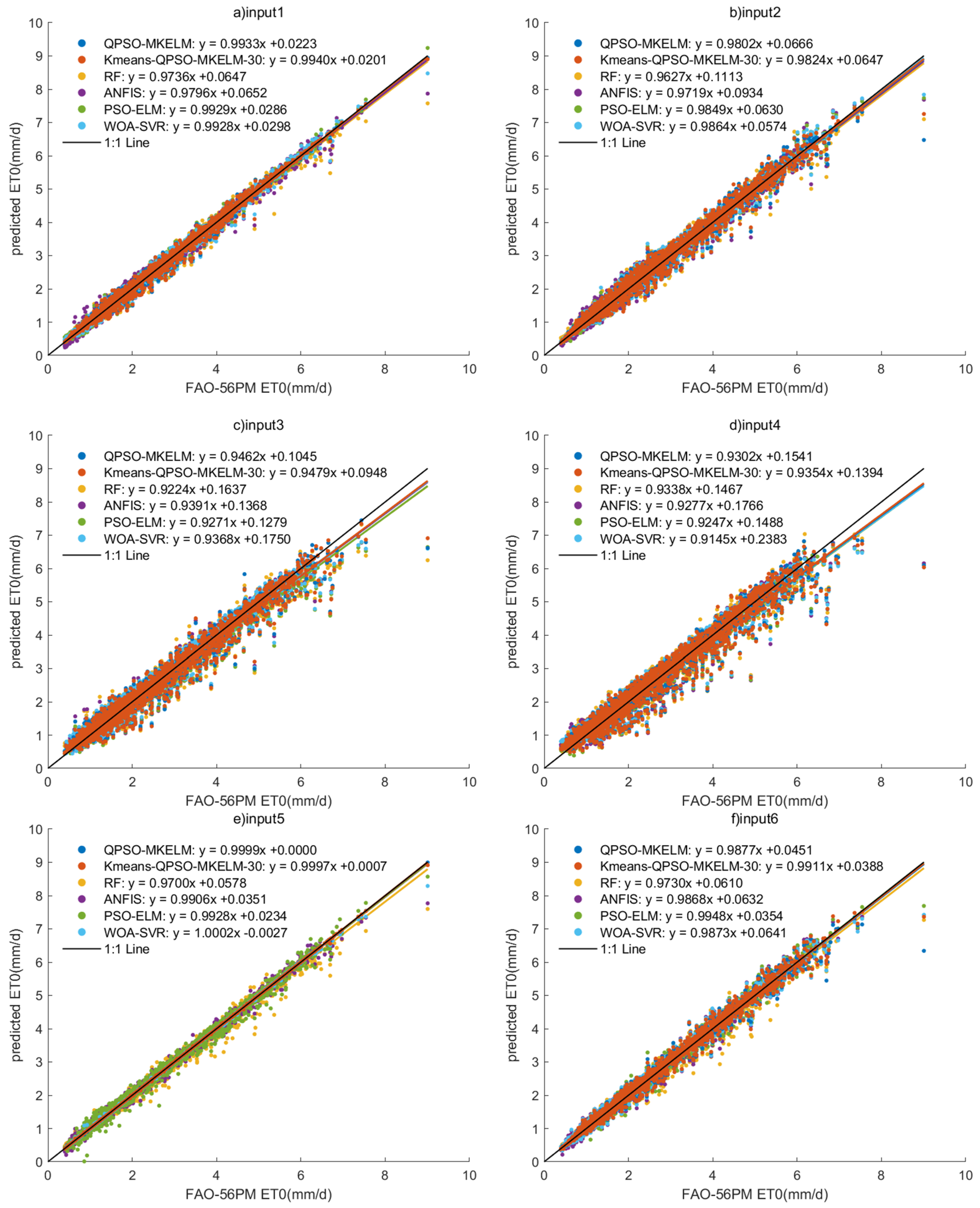
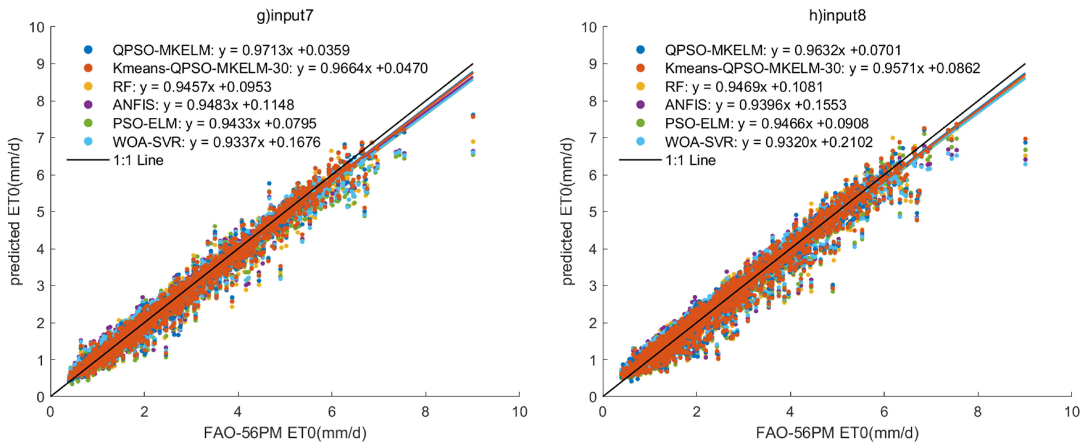
In the comparative experiment, the QPSO-MKELM model, Kmeans-QPSO-MKELM-30 model, ANFIS model, PSO-ELM model, WOA-SVR model (with RBF kernel), and RF model were selected to compare the impact of different input features on ET0 prediction accuracy. The modeling results of these models under eight different input feature sets, including their ET0 prediction accuracy and runtime, are shown in Table 7. Additionally, scatter plots of the models’ predictions under the eight input sets are displayed in Figure 5, and the Taylor diagram is shown in Figure 6.
Table 7.
Error metrics and runtime statistics of each model in the comparative experiment.
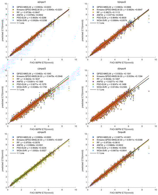

Figure 5.
Scatter plots of prediction results of each model under different inputs in the comparison experiment.
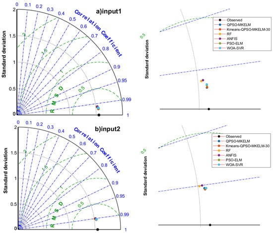
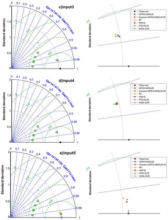
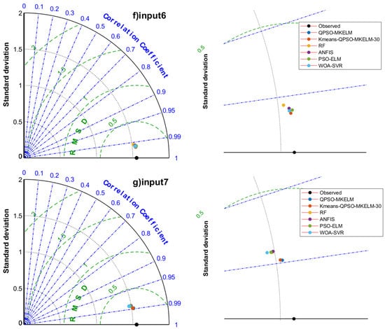
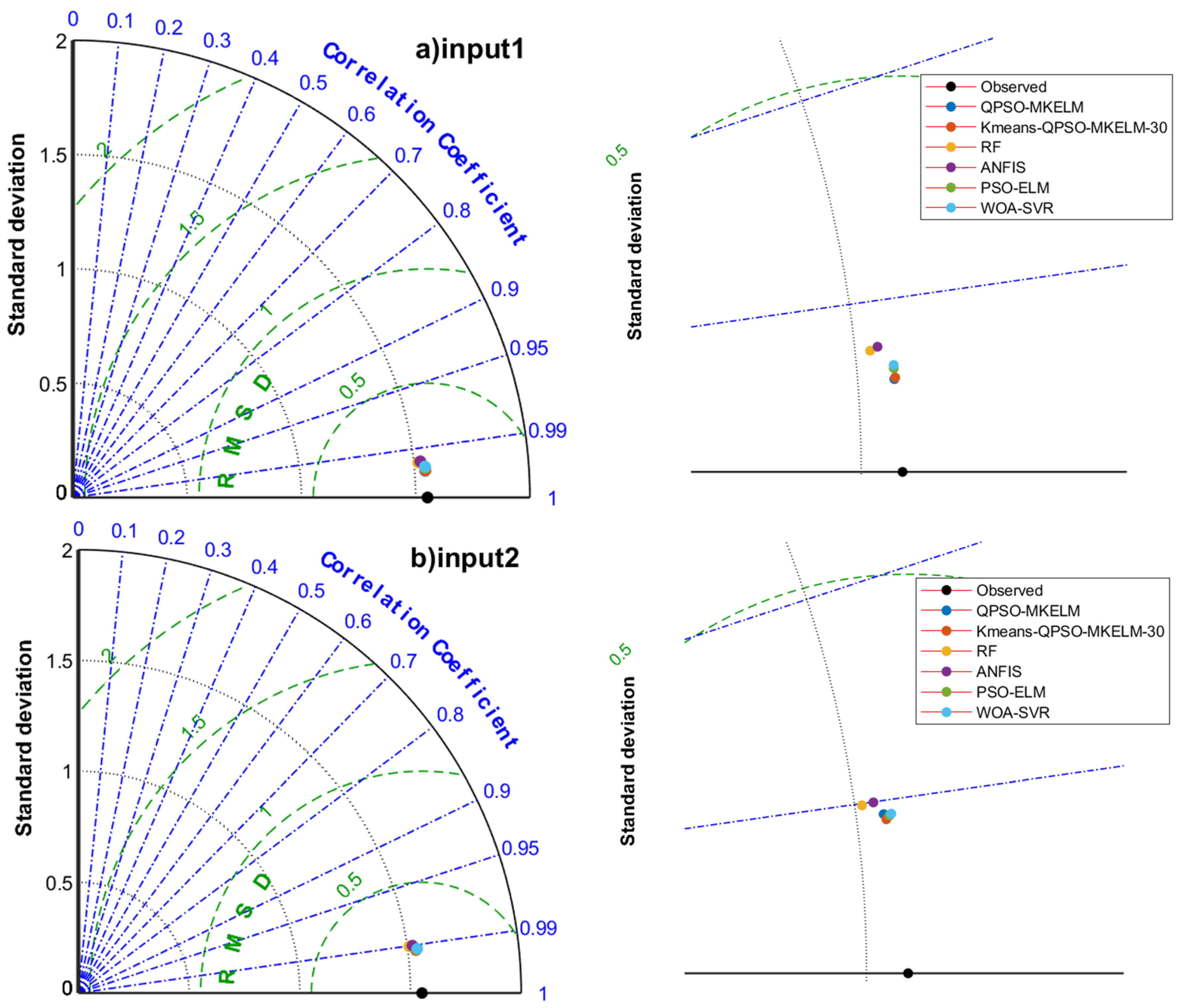
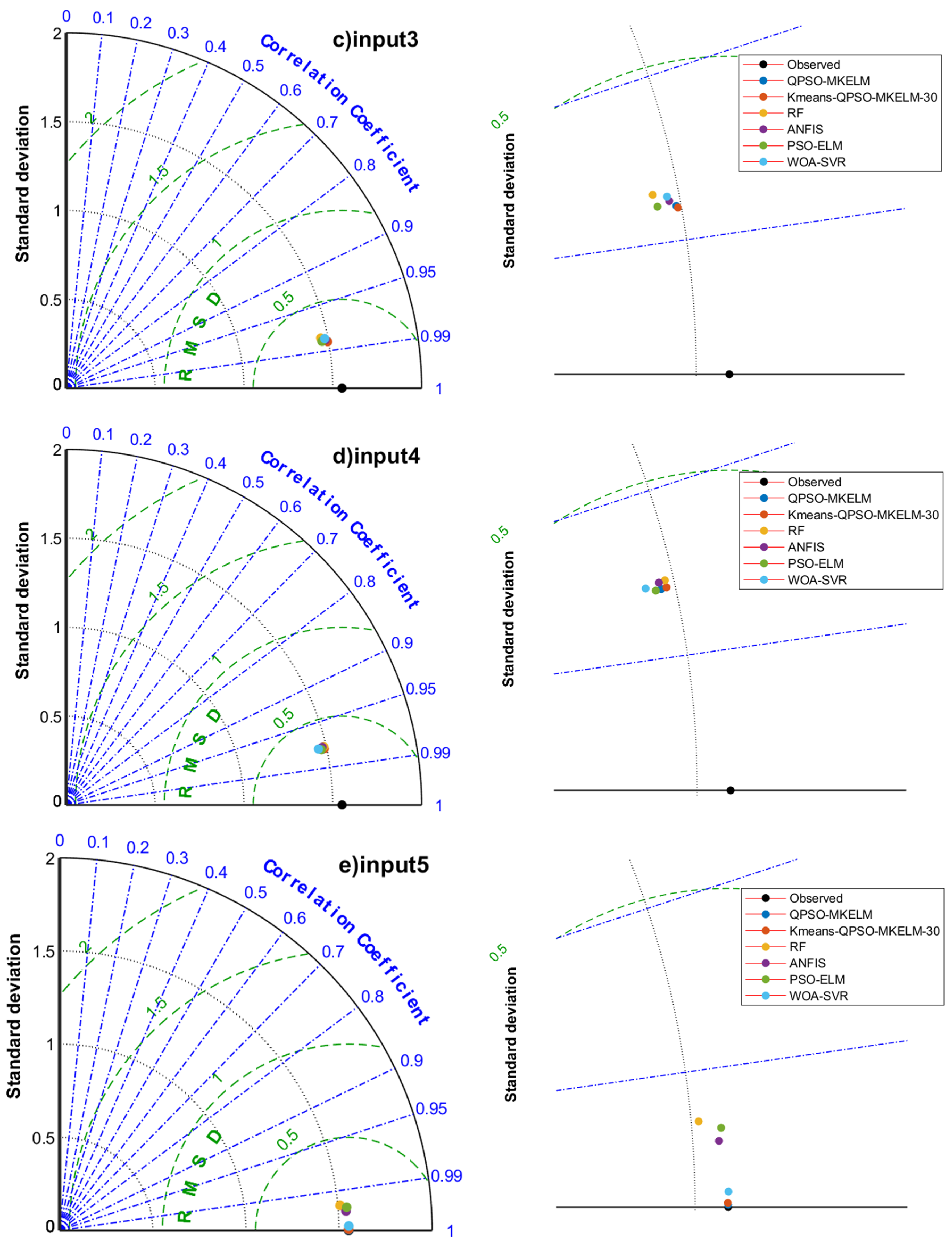
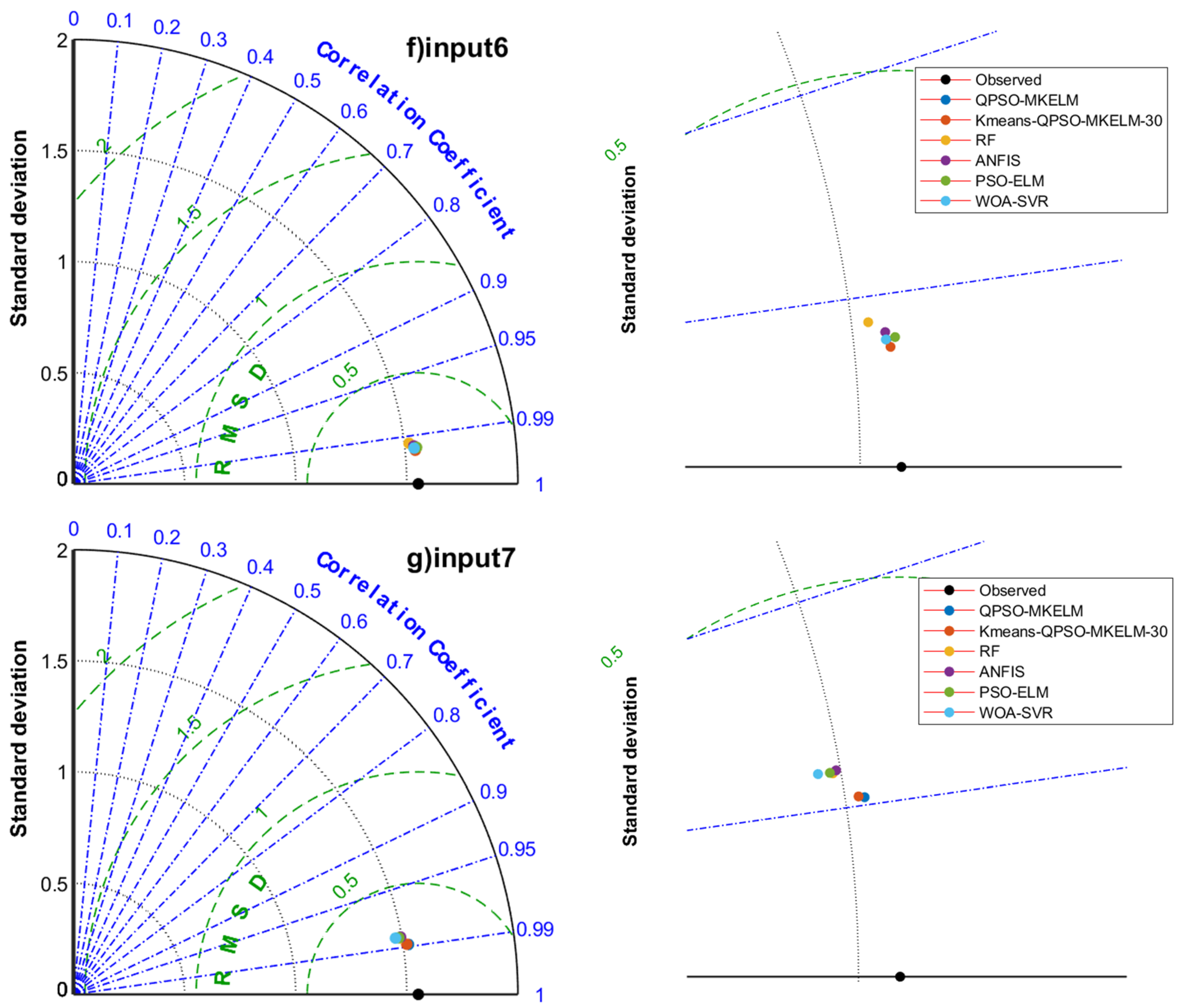
Figure 6.
Taylor diagrams of prediction results of each model under different inputs in the comparison experiment.
- Effect of different feature inputs on model prediction accuracy: The combination of temperature, humidity, and sunlight duration (input 2, input 6) outperformed the combination of temperature, wind speed, and sunlight duration (input 3, input 7) regarding prediction accuracy. For input 5, the predicted R2 values for all models ranged from 0.99135 to 0.99999, MAE from 0.00187 to 0.08962 mm, and RMSE from 0.00390 to 0.14437 mm. In the scatter plot (Figure 5e), the predictions were closely aligned with the 1:1 line, and in the Taylor diagram (Figure 6e), the points were very near the observed values. All models achieved remarkably high accuracy, making input 5 a recommended feature set when sufficient meteorological data are available. For input 8, the predicted R2 values ranged from 0.95739 to 0.9639, MAE from 0.21065 to 0.24072 mm, and RMSE from 0.29486 to 0.32035 mm. The scatter plot (Figure 5h) showed an even distribution with only a few outliers, demonstrating that even with just temperature and sunlight duration as features, the prediction accuracy for ET0 remained relatively high. This result can guide the selection of meteorological features when equipment and budget resources are limited. Adding the date feature to the input significantly improved the prediction accuracy for all models, with only a slight increase in runtime. Therefore, it is recommended that the date feature be included when building predictive models.
- Comparing the prediction accuracy of different models with the same input features, it can be observed that the QPSO-MKELM and Kmeans-QPSO-MKELM-30 models outperform all other models across all input features. These two models are also closer to the observed points on the Taylor diagram (Figure 6). Additionally, by comparing the three error metrics and scatter plots (Table 7 and Figure 5), it is found that the inclusion of the date feature leads to a more significant improvement in prediction accuracy for these two models compared to other models. In the Taylor diagram (Figure 6), the distance between these two models and the target observation point is further reduced by including the date feature. This can be attributed to the fact that the MKELM model’s weighted multi-kernel function is more capable of capturing various data structures and relationships, including the relationship between the date feature and ET0. Particularly in input 5, which includes the most features, the QPSO-MKELM and Kmeans-QPSO-MKELM-30 models almost perfectly fit the 1:1 line in the scatter plot (Figure 5e), and they are the only models without any outliers. The PSO-ELM and WOA-SVR models have similar prediction accuracy, falling in the middle range. They each have strengths and weaknesses depending on the meteorological feature inputs: in inputs 4 and 8, which only include temperature and sunshine duration, the PSO-ELM model performs better, while in inputs 1 and 5, which include humidity and wind speed, the WOA-SVR model performs better. The ANFIS model has slightly lower overall accuracy compared to the two models mentioned earlier. The RF model performs relatively poorly in terms of prediction accuracy, consistently ranking among the bottom two in inputs 1 through 6. It is also farther from the observed values on the Taylor diagram (Figure 6).
- Comparing the running times of different models, it can be observed that the QPSO-MKELM model (18,364–20,932 s) and the WOA-SVR model (3504–4236 s) have significantly longer running times compared to the other models. This is primarily due to the computation of a large kernel matrix. The RF model has the shortest running time, ranging from 96 s to 151 s. The running times of the Kmeans-QPSO-MKELM-30 model (399 s–544 s), PSO-ELM model (500–613 s), and ANFIS model (370–590 s) are within the same range, with the Kmeans-QPSO-MKELM-30 model being slightly faster.
4. Discussion
This study first estimated the importance of meteorological features for predicting ET0 based on the correlation between each meteorological feature and ET0 and the correlation among the meteorological features themselves. The normalized variance values of the features were used to assess their significance, and important features were selected while redundant ones were excluded. The study identified temperature and sunshine duration as the two most important features for estimating evapotranspiration. All models achieved over 95% prediction accuracy in experiments when only temperature and sunshine duration were used as inputs. This is consistent with the findings of Zhao et al. (2023), who predicted evapotranspiration for 14 sites in southern China [48]. This indicates that estimating ET0 using only temperature and sunshine duration in southern China with limited meteorological conditions is reasonable. This finding provides valuable guidance for sensor selection and data collection in practical applications that require ET0 prediction.
Considering that evapotranspiration varies uniformly and exhibits significant periodicity in the study region, the sine and cosine values of the date were added as inputs, resulting in a noticeable improvement in prediction accuracy across all models. Similarly, Hu et al. (2024) incorporated extraterrestrial radiation (Ra), a parameter that can be calculated from the date and latitude, into their model, and observed a significant improvement in prediction performance [49]. Building upon the widely recommended PSO-ELM model for ET0 prediction, this study proposes the Kmeans-QPSO-MKELM algorithm, which addresses the shortcomings of the original model. The new model improves prediction accuracy and achieves a shorter training time. At the research site, the new model outperformed the WOA-SVR model proposed by Mohammadi et al. (2020) for ET0 prediction [24], achieving higher prediction accuracy and shorter training time. The prediction accuracy of the new model was also higher than that of the traditional ANFIS and RF models.
At the same time, this study has several limitations and areas for improvement:
- In this study, the Kmeans-QPSO-MKELM model used a linear kernel function, a polynomial kernel function, and an RBF kernel. Future research could compare the impact of different kernel functions on the model’s ability to capture meteorological features and predict ET0. Given that ET0 exhibits periodicity, periodic kernel functions could be included.
- This study was conducted only in one location within a single climatic zone. Future studies should expand to different climatic zones to assess the model’s performance in varied conditions.
- This study used the FAO-56 model to calculate the target values of ET0, which is a common practice. However, the conclusions drawn may not be robust enough, and therefore, future research should use experimental ET0 data as the target value for more reliable experiments.
- The models compared in this study were limited. Future work could include comparisons with other models, such as deep learning models, to assess their performance.
5. Conclusions
This study proposed eight input models based on the variance and correlation coefficients of meteorological factors combined with the cosine and sine values of the date. To address the shortcomings of the commonly used PSO-ELM model for ET0 prediction, the Kmeans-QPSO-MKELM model was proposed. The optimal number of clusters was selected in the experiment, followed by ablation and comparison experiments. The main conclusions are as follows:
- Compared to the PSO-ELM model, the Kmeans-QPSO-MKELM model, with improvements in the optimization algorithm, reduces the probability of PSO falling into local optima and has a higher chance of finding a better solution. Introducing multiple kernel functions in the ELM model improves its ability to handle complex nonlinear problems, especially when input factors such as wind speed, which exhibit a more nonlinear relationship with ET0, are included. When K-means clustering is applied, and the number of clusters is appropriately chosen, classification training followed by weighted prediction significantly reduces the model training time while maintaining similar prediction accuracy.
- For all models in this study, adding the cosine and sine values of the date as input significantly improved prediction accuracy. It is, therefore, recommended that the cosine and sine values of the date be included in the input features.
- Comparison experiments show that the prediction accuracy of Kmeans-QPSO-MKELM and QPSO-MKELM is significantly higher than that of other models under all eight input scenarios, especially when the date cosine and sine values are included. The Kmeans-QPSO-MKELM model runs slightly slower than the RF model but faster than all other models in the comparison. Therefore, it is strongly recommended to use the Kmeans-QPSO-MKELM model combined with the date cosine and sine values as inputs for ET0 prediction.
Author Contributions
Conceptualization, C.Z.; methodology, C.Z. and M.Y.; software, C.Z.; validation, C.Z.; formal analysis, C.Z.; data curation, C.Z.; writing—original draft preparation, C.Z.; writing—review and editing, C.Z. and M.Y.; visualization, C.Z.; supervision, M.Y. All authors have read and agreed to the published version of the manuscript.
Funding
This research received no external funding.
Institutional Review Board Statement
Not applicable.
Informed Consent Statement
Not applicable.
Data Availability Statement
The data that support the findings of this study are available from the corresponding authors upon reasonable request.
Conflicts of Interest
The authors declare no conflicts of interest.
References
- Zhao, J.; Xia, H.; Yue, Q.; Wang, Z. Spatiotemporal variation in reference evapotranspiration and its contributing climatic factors in China under future scenarios. Int. J. Climatol. 2020, 40, 3813–3831. [Google Scholar] [CrossRef]
- Valipour, M.; Khoshkam, H.; Bateni, S.M.; Jun, C.; Band, S.S. Hybrid machine learning and deep learning models for multi-step-ahead daily reference evapotranspiration forecasting in different climate regions across the contiguous United States. Agric. Water Manag. 2023, 283, 108311. [Google Scholar] [CrossRef]
- Zhao, T.; Wang, Q.J.; Schepen, A.; Griffiths, M. Ensemble forecasting of monthly and seasonal reference crop evapotranspiration based on global climate model outputs. Agric. For. Meteorol. 2019, 264, 114–124. [Google Scholar] [CrossRef]
- Ahmadi, F.; Mehdizadeh, S.; Mohammadi, B.; Pham, Q.B.; Doan, T.N.C.; Vo, N.D. Application of an artificial intelligence technique enhanced with intelligent water drops for monthly reference evapotranspiration estimation. Agric. Water Manag. 2021, 244, 106622. [Google Scholar] [CrossRef]
- Allen, R.G.; Pereira, L.S.; Raes, D.; Smith, M. Crop Evapotranspiration: Guidelines for Computing Crop Requirements. FAO Irrig. Drain. Pap. 56 1998, 300, D05109. [Google Scholar]
- Ponraj, A.S.; Vigneswaran, T. Daily evapotranspiration prediction using gradient boost regression model for irrigation planning. J. Supercomput. 2020, 76, 5732–5744. [Google Scholar] [CrossRef]
- Zhou, Z.G.; Zhao, L.; Lin, A.W.; Qin, W.M.; Lu, Y.B.; Li, J.Y.; Zhong, Y.; He, L.J. Exploring the potential of deep factorization machine and various gradient boosting models in modeling daily reference evapotranspiration in China. Arab. J. Geosci. 2020, 13, 1287. [Google Scholar] [CrossRef]
- Saggi, M.K.; Jain, S. Reference evapotranspiration estimation and modeling of the Punjab Northern India using deep learning. Comput. Electron. Agric. 2019, 156, 387–398. [Google Scholar] [CrossRef]
- Roy, D.K.; Barzegar, R.; Quilty, J.; Adamowski, J. Using ensembles of adaptive neuro-fuzzy inference system and optimization algorithms to predict reference evapotranspiration in subtropical climatic zones. J. Hydrol. 2020, 591, 125509. [Google Scholar] [CrossRef]
- Dong, J.H.; Liu, X.G.; Huang, G.M.; Fan, J.L.; Wu, L.F.; Wu, J. Comparison of four bio-inspired algorithms to optimize KNEA for predicting monthly reference evapotranspiration in different climate zones of China. Comput. Electron. Agric. 2021, 186, 106211. [Google Scholar] [CrossRef]
- Salam, R.; Islam, A.M.T. Potential of RT, bagging and RS ensemble learning algorithms for reference evapotranspiration prediction using climatic data-limited humid region in Bangladesh. J. Hydrol. 2020, 590, 125241. [Google Scholar]
- Zhu, B.; Feng, Y.; Gong, D.; Jiang, S.; Zhao, L.; Cui, N. Hybrid particle swarm optimization with extreme learning machine for daily reference evapotranspiration prediction from limited climatic data. Comput. Electron. Agric. 2020, 173, 105430. [Google Scholar]
- Wu, Z.; Cui, N.; Hu, X.; Gong, D.; Wang, Y.; Feng, Y.; Jiang, S.; Lv, M.; Han, L.; Xing, L.; et al. Optimization of extreme learning machine model with biological heuristic algorithms to estimate daily reference crop evapotranspiration in different climatic regions of China. J. Hydrol. 2021, 603, 127028. [Google Scholar] [CrossRef]
- Djaman, K.; Balde, A.B.; Sow, A.; Muller, B.; Irmak, S.; N’Diaye, M.K.; Manneh, B.; Moukoumbi, Y.D.; Futakuchi, K.; Saito, K. Evaluation of sixteen reference evapotranspiration methods under sahelian conditions in the Senegal River Valley. J. Hydrol. Reg. Stud. 2015, 3, 139–159. [Google Scholar]
- Wu, Z.; Chen, X.; Cui, N.; Zhu, B.; Gong, D.; Han, L.; Xing, L.; Zhen, S.; Li, Q.; Liu, Q.; et al. Optimized empirical model based on whale optimization algorithm for simulate daily reference crop evapotranspiration in different climatic regions of China. J. Hydrol. 2022, 612, 128084. [Google Scholar]
- Duhan, D.; Singh, M.C.; Singh, D.; Satpute, S.; Singh, S.; Prasad, V. Modeling reference evapotranspiration using machine learning and remote sensing techniques for semiarid subtropical climate of Indian Punjab. J. Water Clim. Change 2023, 14, 2227–2243. [Google Scholar]
- Fan, J.; Yue, W.; Wu, L.; Zhang, F.; Cai, H.; Wang, X.; Lu, X.; Xiang, Y. Evaluation of SVM, ELM and four tree-based ensemble models for predicting daily reference evapotranspiration using limited meteorological data in different climates of China. Agric. For. Meteorol. 2018, 263, 225–241. [Google Scholar] [CrossRef]
- Wu, L.; Fan, J. Comparison of neuron-based, kernel-based, tree-based and curve-based machine learning models for predicting daily reference evapotranspiration. PLoS ONE 2019, 14, e0217520. [Google Scholar] [CrossRef]
- Khoja, I.; Latrech, B.; Lasram, A.; Ladhari, T.; M’Sahli, F.; Sakly, A. Application of Machine Learning in Agriculture the Reference Evapotranspiration Model Prediction. In Proceedings of the 2023 IEEE International Conference on Artificial Intelligence & Green Energy, Sousse, Tunisia, 12–14 October 2023. [Google Scholar]
- Huang, G.; Huang, G.B.; Song, S.J.; You, K.Y. Trends in extreme learning machines: A review. Neural Netw. 2015, 61, 32–48. [Google Scholar]
- Abdullah, S.S.; Malek, M.A.; Abdullah, N.S.; Kisi, O.; Yap, K.S. Extreme Learning Machines: A new approach for prediction of reference evapotranspiration. J. Hydrol. 2015, 527, 184–195. [Google Scholar] [CrossRef]
- Kumar, D.; Adamowski, J.; Suresh, R.; Ozga-Zielinski, B. Estimating Evapotranspiration Using an Extreme Learning Machine Model: Case Study in North Bihar, India. J. Irrig. Drain. Eng. 2016, 142, 04016032. [Google Scholar]
- Qin, A.Z.; Fan, Z.L.; Zhang, L.Z. Hybrid Genetic Algorithm-Based BP Neural Network Models Optimize Estimation Performance of Reference Crop Evapotranspiration in China. Appl. Sci.-Basel 2022, 12, 10689. [Google Scholar]
- Mohammadi, B.; Mehdizadeh, S. Modeling daily reference evapotranspiration via a novel approach based on support vector regression coupled with whale optimization algorithm. Agric. Water Manag. 2020, 237, 106145. [Google Scholar] [CrossRef]
- Zhao, L.; Zhao, X.; Pan, X.; Shi, Y.; Qiu, Z.; Li, X.; Xing, X.; Bai, J. Prediction of daily reference crop evapotranspiration in different Chinese climate zones: Combined application of key meteorological factors and Elman algorithm. J. Hydrol. 2022, 610, 127822. [Google Scholar] [CrossRef]
- Shi, Y.; Wang, Y.; Zhao, L.; Cao, R.; Wang, Y.; Shen, J.; Duan, Z. Evapotranspiration prediction using CART importance ranking and hybrid ELM models. Trans. Chin. Soc. Agric. Eng. 2023, 39, 89–96. [Google Scholar]
- Jun, S.; Bin, F.; Wenbo, X. Particle swarm optimization with particles having quantum behavior. In Proceedings of the 2004 Congress on Evolutionary Computation, Portland, OR, USA, 19–23 June 2004. [Google Scholar]
- Wang, C.T.; Li, W.; Xin, G.F.; Wang, Y.Q.; Xu, S.Y. Prediction Model of Corrosion Current Density Induced by Stray Current Based on QPSO-Driven Neural Network. Complexity 2019, 2019, 3429816. [Google Scholar]
- Alajmi, M.S.; Almeshal, A.M. Least Squares Boosting Ensemble and Quantum-Behaved Particle Swarm Optimization for Predicting the Surface Roughness in Face Milling Process of Aluminum Material. Appl. Sci.-Basel 2021, 11, 2126. [Google Scholar]
- Shi, H.C.; Shi, M.L.; Xu, W.S. Cable Tension of Long-Span Steel Box Tied Arch Bridges Based on Radial Basis Function-Support Vector Machine Optimized by Quantum-Behaved Particle Swarm Optimization. Appl. Sci.-Basel 2024, 14, 7163. [Google Scholar]
- Zhao, L.; Zhao, X.B.; Li, Y.Z.; Shi, Y.; Zhou, H.M.; Li, X.Z.; Wang, X.D.; Xing, X.G. Applicability of hybrid bionic optimization models with kernel-based extreme learning machine algorithm for predicting daily reference evapotranspiration: A case study in arid and semiarid regions, China. Environ. Sci. Pollut. Res. 2023, 30, 22396–22412. [Google Scholar]
- Wu, L.F.; Peng, Y.W.; Fan, J.L.; Wang, Y.C.; Huang, G.M. A novel kernel extreme learning machine model coupled with K-means clustering and firefly algorithm for estimating monthly reference evapotranspiration in parallel computation. Agric. Water Manag. 2021, 245, 106624. [Google Scholar]
- Li, T.Y.; Qian, Z.J.; He, T. Short-Term Load Forecasting with Improved CEEMDAN and GWO-Based Multiple Kernel ELM. Complexity 2020, 2020, 1209547. [Google Scholar] [CrossRef]
- Ma, L.; Li, J. Short-term wind power prediction based on multiple kernel extreme learning machine method. In Proceedings of the 2020 7th International Forum on Electrical Engineering and Automation, Hefei, China, 25–27 September 2020. [Google Scholar]
- Zhang, Y.D.; Ma, H.Y.; Wang, S.; Li, S.Y.; Guo, R. Indirect prediction of remaining useful life for lithium-ion batteries based on improved multiple kernel extreme learning machine. J. Energy Storage 2023, 64. [Google Scholar] [CrossRef]
- Shen, Y.P.; Zheng, K.F.; Wu, C.H.; Yang, Y.X. A Nature-inspired Multiple Kernel Extreme Learning Machine Model for Intrusion Detection. Ksii Trans. Internet Inf. Syst. 2020, 14, 702–723. [Google Scholar]
- Feng, Y.; Cui, N.; Gong, D.; Zhang, Q.; Zhao, L. Evaluation of random forests and generalized regression neural networks for daily reference evapotranspiration modelling. Agric. Water Manag. 2017, 193, 163–173. [Google Scholar]
- Black, J.N.; Bonython, C.W.; Prescott, J.A. Solar radiation and the duration of sunshine. Q. J. R. Meteorol. Soc. 1954, 80, 231–235. [Google Scholar]
- Reshef, D.N.; Reshef, Y.A.; Finucane, H.K.; Grossman, S.R.; McVean, G.; Turnbaugh, P.J.; Lander, E.S.; Mitzenmacher, M.; Sabeti, P.C. Detecting novel associations in large data sets. Science 2011, 334, 1518–1524. [Google Scholar]
- Huang, G.B.; Zhu, Q.Y.; Siew, C.K. Extreme learning machine: Theory and applications. Neurocomputing 2006, 70, 489–501. [Google Scholar] [CrossRef]
- Huang, G.B. An Insight into Extreme Learning Machines: Random Neurons, Random Features and Kernels. Cogn. Comput. 2014, 6, 376–390. [Google Scholar] [CrossRef]
- Chai, T.; Draxler, R.R. Root mean square error (RMSE) or mean absolute error (MAE)? —Arguments against avoiding RMSE in the literature. Geosci. Model Dev. 2014, 7, 1247–1250. [Google Scholar]
- Hodson, T.O. Root-mean-square error (RMSE) or mean absolute error (MAE): When to use them or not. Geosci. Model Dev. 2022, 15, 5481–5487. [Google Scholar]
- Heramb, P.; Rao, K.V.R.; Subeesh, A.; Srivastava, A. Predictive Modelling of Reference Evapotranspiration Using Machine Learning Models Coupled with Grey Wolf Optimizer. Water 2023, 15, 856. [Google Scholar] [CrossRef]
- Cemek, B.; Tasan, S.; Canturk, A.; Tasan, M.; Simsek, H. Machine learning techniques in estimation of eggplant crop evapotranspiration. Appl. Water Sci. 2023, 13, 136. [Google Scholar] [CrossRef]
- Cheshmberah, F.; Zolfaghari, A.A. The Effect of Climate Change on Future Reference Evapotranspiration in Different Climatic Zones of Iran. Pure Appl. Geophys. 2019, 176, 3649–3664. [Google Scholar] [CrossRef]
- Wang, G.T.; Zhao, X.J.; Zhang, Z.H.; Song, S.L.; Wu, Y.Y. Machine learning-based estimation of evapotranspiration under adaptation conditions: A case study in Heilongjiang Province, China. Int. J. Biometeorol. 2024, 68, 2543–2564. [Google Scholar] [CrossRef] [PubMed]
- Zhao, L.; Xing, L.W.; Wang, Y.H.; Cui, N.B.; Zhou, H.M.; Shi, Y.; Chen, S.D.; Zhao, X.B.; Li, Z. Prediction Model for Reference Crop Evapotranspiration Based on the Back-propagation Algorithm with Limited Factors. Water Resour. Manag. 2023, 37, 1207–1222. [Google Scholar] [CrossRef]
- Hu, J.; Ma, R.; Jiang, S.Z.; Liu, Y.L.; Mao, H.Y. Prediction of Reference Crop Evapotranspiration in China’s Climatic Regions Using Optimized Machine Learning Models. Water 2024, 16, 3349. [Google Scholar] [CrossRef]


Disclaimer/Publisher’s Note: The statements, opinions and data contained in all publications are solely those of the individual author(s) and contributor(s) and not of MDPI and/or the editor(s). MDPI and/or the editor(s) disclaim responsibility for any injury to people or property resulting from any ideas, methods, instructions or products referred to in the content. |
© 2025 by the authors. Licensee MDPI, Basel, Switzerland. This article is an open access article distributed under the terms and conditions of the Creative Commons Attribution (CC BY) license (https://creativecommons.org/licenses/by/4.0/).