1. Introduction
The International Thermonuclear Experimental Reactor (ITER), under construction in Cadarche, in Southern France, aims to create a sustained deuterium/tritium plasma predominantly heated by α particles, thus proving the technological and scientific feasibility of fusion power reactors [
1,
2].
The reference plasma scenario for the ITER’s operation is the high-confinement state (H-mode) [
3], with a longer energy confinement time than in the low-confinement state (L-mode); the latter one is characterised by relatively higher turbulence, which allows the energy to escape the plasma [
4]. The H-mode provides the basis for achieving a net gain of the reactor of up to 10 (Q = 10), with 500 MW of fusion power from 50 MW of input heating power [
5].
The DINA code has been developed for the simulation of the plasma scenario [
5], and it has been validated with experiments [
6,
7]. Simulations of the plasma burn in the ITER reactor were provided for two representative scenarios of ITER operation [
8]. The first scenario has a 15 MA plasma current with a full-bore plasma producing 500 MW of fusion power with Q = 10 for about 400 s. The second scenario is a steady-state case with a plasma current of 9 MA and a highly shaped plasma, producing about 300 MW of fusion power with a net gain higher than 5 (Q > 5) for about 3000 s [
2].
During the plasma scenario, several loss sources arise, which involve the superconducting coils, cooled by supercritical helium (SHe), and the cryogenic system. The major contributors are as follows.
Maintaining the superconducting magnets within a controlled temperature increase is crucial for the safe operation of the reactor. An uncontrolled temperature rise can lead to the current-sharing temperature threshold being exceeded, generating Joule heating and then an irreversible quench during plasma operation [
16,
17].
Adequate numerical modelling of the superconducting magnets during plasma scenarios is crucial in estimating the operational temperature margin of the coils and preventing permanent damage to the magnet [
18]. The challenge of these analyses, when using numerical methods, is related to two main aspects:
The model requires a multi-physics analysis, able to tackle thermal, hydraulic and electromagnetic phenomena;
A large number of degrees of freedom is required to discretise a large-scale magnet, wound with several kilometres of cable-in-conduit conductors (CICCs), and its cryogenic system, with several kilometres of pipes and different components, such as bypass and control valves, heat exchangers and the circulation pump.
Several numerical models have been developed from the 1980s to the present day, with the intent to analyse the multi-physics behaviour of a superconducting magnet: from the early works with MAGS [
19] or Saruman/Gandalf [
20,
21] to the most recent models with Vincenta/Venezia [
22,
23], the 4C code [
24,
25] and
SuperMagnet [
26,
27].
In this work, the temperature margin—here defined as the difference between the temperature in the conductor and the current-sharing temperature—and, more generally, the thermal–hydraulic behaviour of the ITER central solenoid (CS) during the 15 MA plasma scenario, modelled with the DINA code, are computed with the
SuperMagnet code [
28]. The
SuperMagnet (SM) code was developed by
CryoSoft [
29] with the intent to simultaneously simulate the electrical, thermal and hydraulic phenomena occurring in superconducting coils [
30].
A methodology is here proposed to reduce the computational burden while still being able to retain the main phenomena occurring during the plasma scenario. The temperature evolution of the conductor and of the supercritical helium—which allows the determination of the operation margin of the conductors—is presented during the plasma scenario. The cryogenic system’s behaviour, with regard to equipment such as the circulation pump and heat exchanger, is also described in detail.
2. The ITER Central Solenoid and the Cryogenic Plant
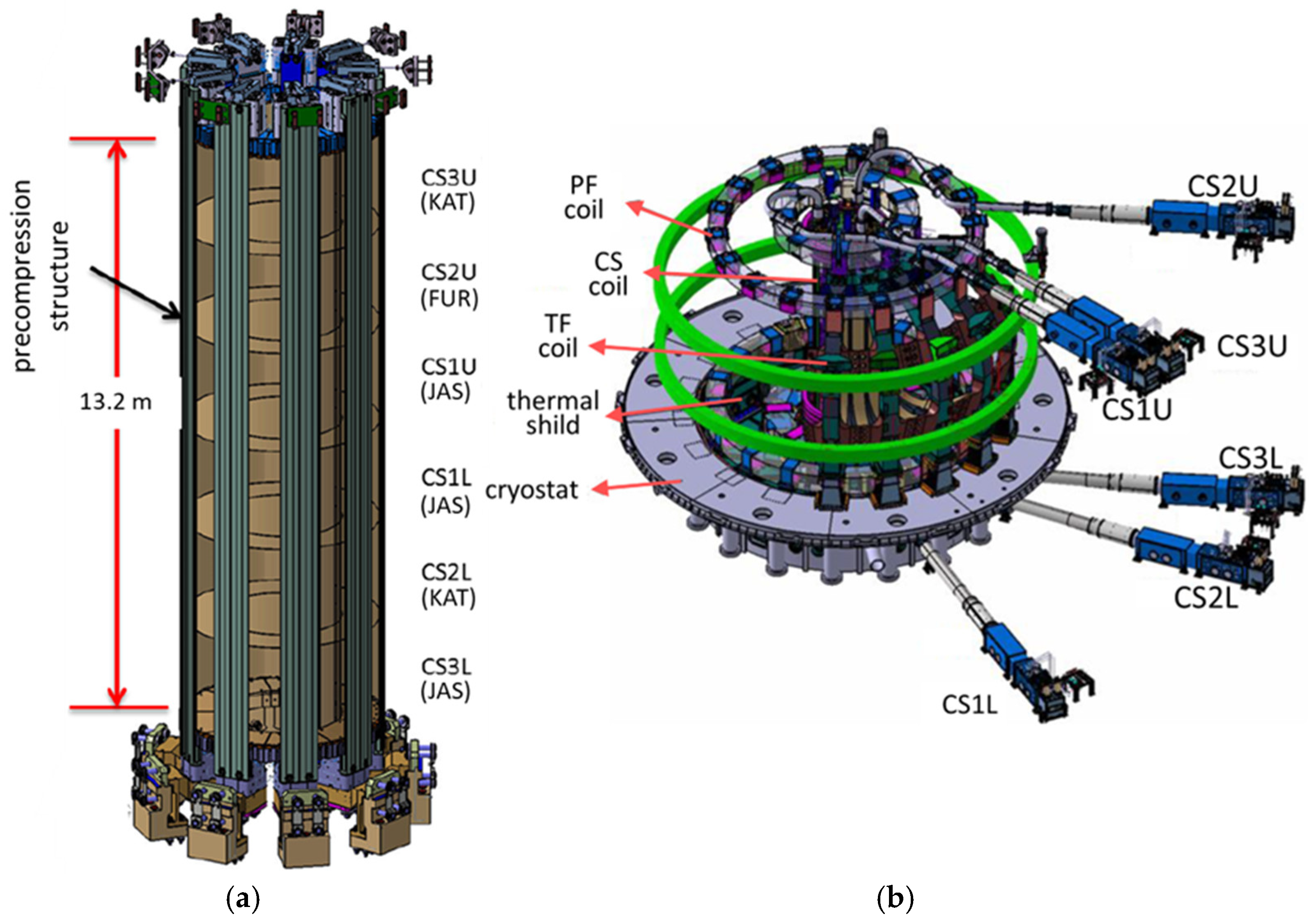
The CS system is composed of six coils [
31,
32] and its feeders with the associated cryogenic cooling loop, as shown in
Figure 1 [
33,
34].
The CS assembly consists of a stack of six identical circular coils, called modules CS3L (bottom lower module) to CS3U (top upper module), compressed together by a mechanical structure and attached to the toroidal field coils (TF) through a supporting system and centring system; see
Figure 1a. The assembly has a diameter of 4.3 m and a height of more than 16 m. Each module is composed of 20 double pancakes (40 pancakes in total) [
34].
The modules are cooled with supercritical He (SHe) at 4.3 K in parallel by their feeders, as shown in
Figure 1b. This loop is closed and independent of any other supercritical loops from the hydraulic point of view [
34].
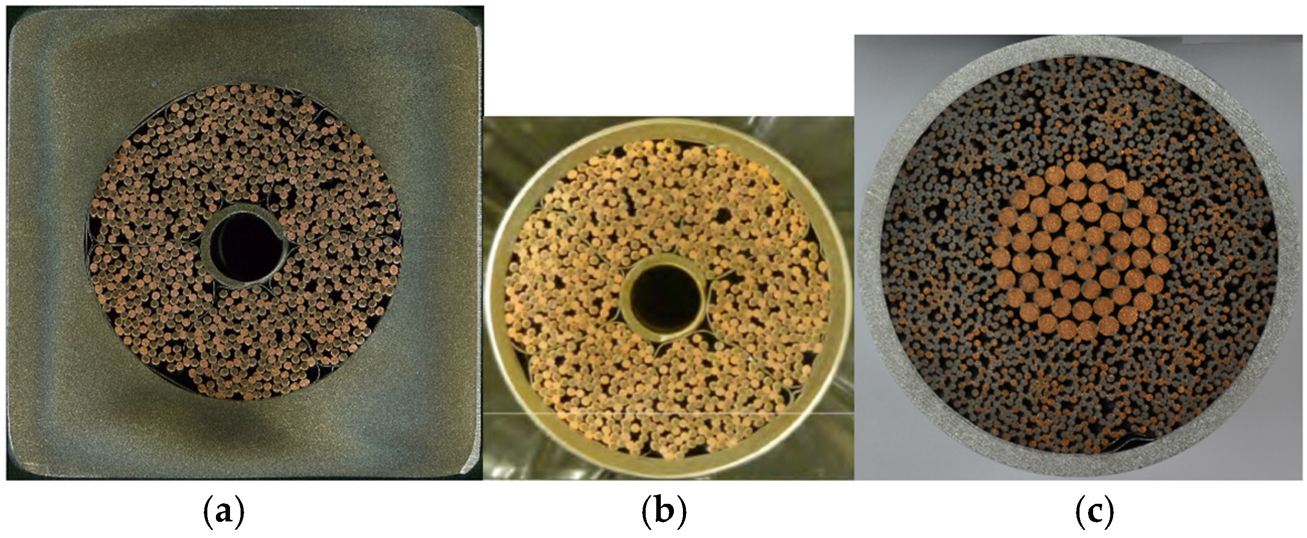
In the CS modules, three different conductor types are used: the conductors in the modules (see
Figure 2a), the busbar lead extensions (EXT; see
Figure 2b) and the main busbar conductors (MB; see
Figure 2c). The conductors in the modules and the lead extensions are manufactured as round cables in a square stainless-steel jacket, while the main busbars are manufactured as round cables in a round stainless-steel jacket. The different strands and corresponding manufacturers used in the aforementioned conductors are reported in
Table 1. The main busbars are manufactured with NbTi strands produced by the Western Superconducting Technologies Co., Ltd. (WST, Xi’an, China). The lead extensions (EXT) and the CS modules are produced with Nb
3Sn strands manufactured by Jastec (JAS, Hyogo, Japan), Furukawa (FUR, Tokyo, Japan) and Kiswire Advanced Technology (KAT, Daejeon, Republic of Korea); they have two main differences:
The conductor realised with KAT strands has a slightly larger central spiral—8 mm × 10 mm instead of 7 mm × 9 mm—which implies different helium sections and void fractions;
The JAS and FUR strands are based on the bronze route process, whereas KAT is based on the internal tin route, and they exhibit slightly different performance (Tcs, AC loss characteristic, etc.).
In the bronze route process, niobium (Nb) filaments are embedded inside the bronze matrix (Cu-Sn alloy) used as the tin source. Instead, in the internal tin route, pure tin (Sn) is used as a direct source, instead of a bronze alloy. During heat treatment, the tin in the bronze diffuses into the Nb filaments, forming Nb3Sn at the Nb–bronze interface. In the internal tin route, the higher tin content leads to faster and more complete Nb3Sn formation. Typically, this results in a higher critical current density (Jc) than in the bronze route. However, the mechanical properties can be weaker compared to those of bronze route wires.
The CS modules, except for the two central ones (CS1U and CS1L), have independent power supplies [
33,
34], used forplasma current initiation, positioning and shaping control. The two central modules of the CS are connected in series to a common power unit.
3. Model Description
3.1. Model of the Cryogenic Plant in Flower
The
Flower model [
35] is a 1D hydraulic tool for the simulation of standard components of cryogenic circuits (heat exchangers, pumps, valves, etc.), combined in a closed hydraulic network [
36,
37]. The
Flower model describes the general hydraulic loop: the pipes, cryogenic pump, heat exchanger, cryogenic lines, feeder, control and bypass valves.
A sketch of the main cryogenic system implemented in
Flower is shown in
Figure 3a. Each module is detailed, with its corresponding feeder and conductors. The general hydraulic scheme of the module and feeder, with details of the joint location, is reported in
Figure 3b.
3.2. Model of the CICC in Thea
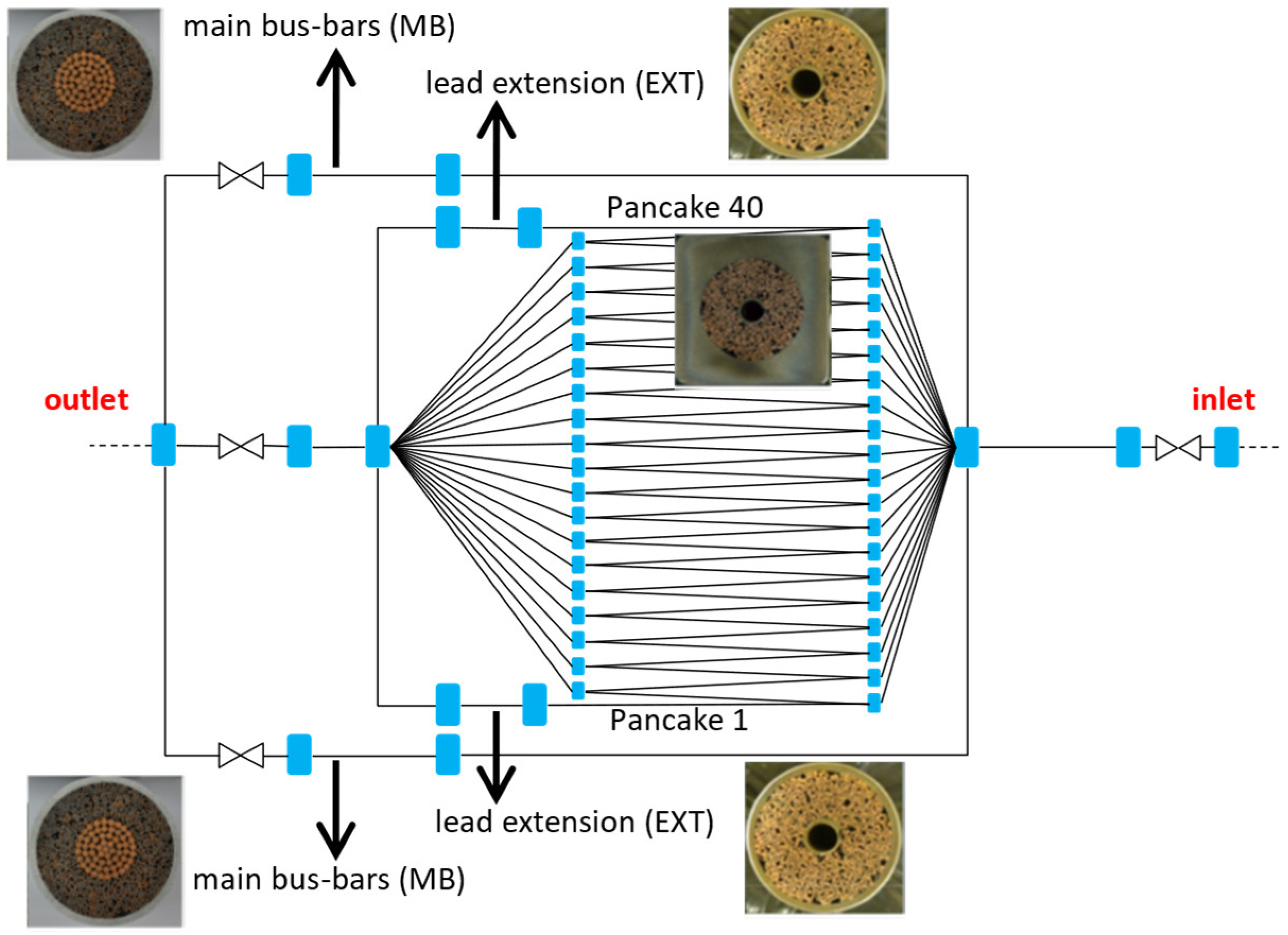
The
Thea model [
38] is a 1D multi-physics tool for the analysis of superconducting cables that accounts for the heat conduction in the solid, the heat transfer in the coolant and the electrical properties of the conductor [
39,
40]. The
Thea model describes the cable-in-conduit conductors (CICCs) with the characteristics of the conductor, the bundle and the spiral. As sketched in
Figure 4, in
Thea, the following conductors are modelled:
CS conductors, with 240 conductors in total and 40 pancakes per module;
Lead extensions (EXT), with 12 in total;
The main busbars (MB), with 12 in total.
In this model, the critical current of the conductors is computed as a function of the magnetic flux density, the temperature and the strain [
41].
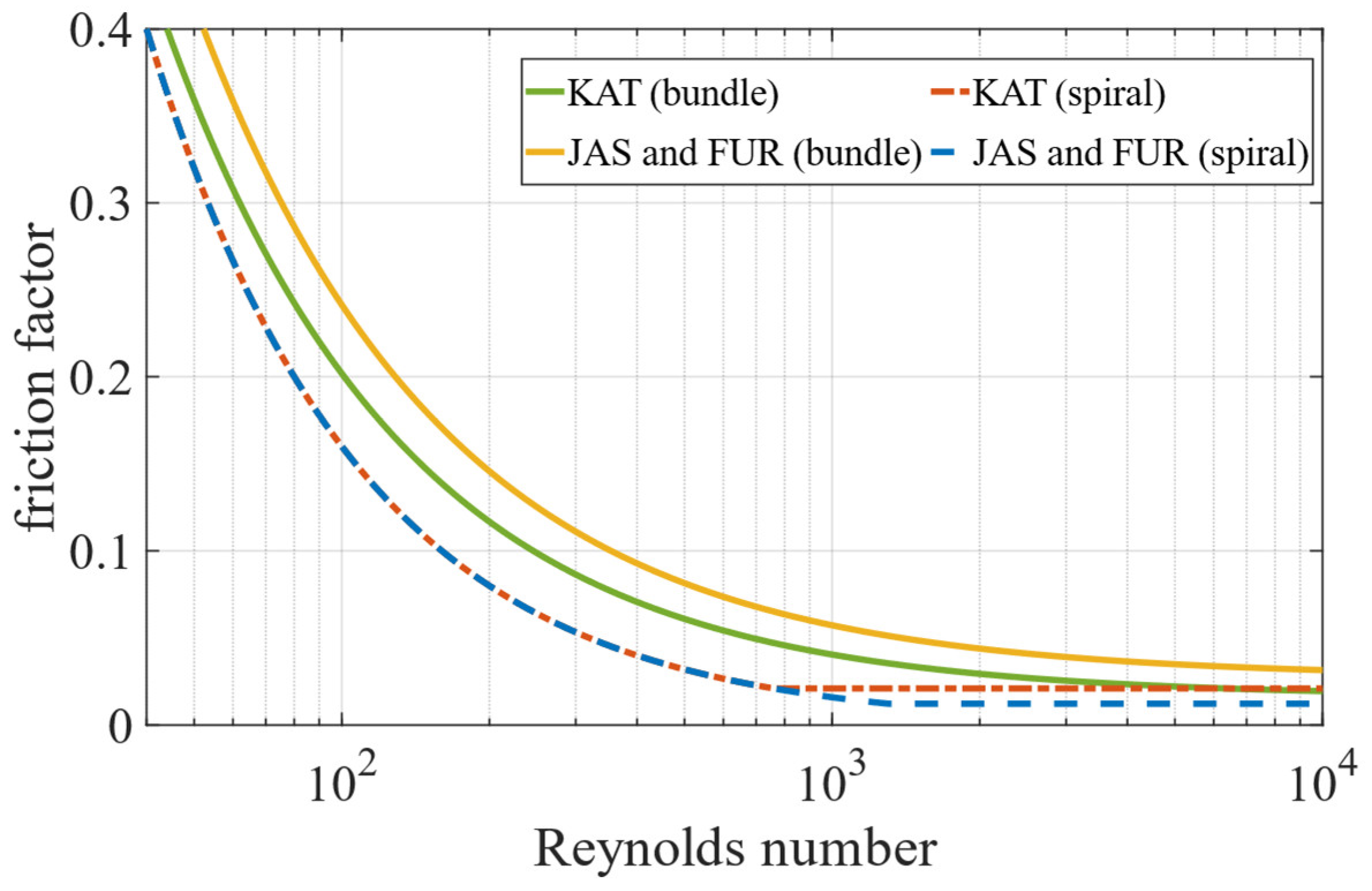
3.2.1. Friction Factor
The friction factor is defined differently in the bundle and in the spiral of the CICCs manufactured with Jastec (JAS), Kiswire (KAT) and Furukawa (FUR) strands according to the following relations.
In the bundle, the Katheder correlation is used [
42]:
where
is the void fraction and
the Reynolds number. The parameters
,
,
and
are reported in
Table 2.
In the spiral, the following relation is implemented [
43]:
and the parameters
and
are collected in
Table 2 for the spiral.
The friction factor as a function of the Reynolds number is shown in
Figure 5 for the different conductor types. The formulations mentioned above are derived by fitting the pressure drop measured during the test campaign of the CS insert [
44], tested in 2016 at the National Institutes for Quantum and Radiological Science and Technology (Naka, Japan), and the CS modules, tested at the premises of General Atomics (Poway, San Diego, CA, USA) [
45,
46].
3.2.2. Strain
The critical current density of the superconducting strands is a crucial parameter describing its electromagnetic characteristics. In Nb3Sn CICCs, the critical current density is a function of the temperature, magnetic field and strain. The concept of the effective strain, defined as the value of uniform strain that determines a given value of the current-sharing temperature of the conductor, is adopted here.
The effective strain in the conductors is modelled according to relation (3). The impact of the transverse force (I × B-dependent component) on the effective strain was assessed from tests of straight samples in the SULTAN facility (SPC, Villigen, Switzerland) in cycled conditions [
47,
48]. In Equation (3), a fraction of the hoop strain—equal to 80%, as established in the test campaign of the CS insert [
49]—is considered:
where
is the cooldown strain, which is usually compressive;
represents the lateral compressive force that crushes the cable against the jacket (proportional to the product of I × B with the current values in Amps). The parameters
,
and
are reported in
Table 3 for the JAS, FUR and KAT conductors. Since the hoop strain map is not available for the plasma scenario, it is not considered (
= 0%). The current-sharing temperature and temperature margin are thus computed under the conservative assumption of no improvement in the conductor’s performance due to the tensile hoop strain.
3.3. Model of the Jacked and Insulation Layers in Heater
The
Heater model [
50] is a 2D finite element model describing the thermal behaviour of the CS stack, accounting for the jacket and the upper and lower insulation plates.
Heater is able to model the 2D diffusion between pancakes and between turns. The 2D mesh includes nine identical cross-sections of the CS stack for each module [
30], equally spaced at an angular distance of 40°, as shown in
Figure 6. The mesh discretises the following parts of the winding:
The stainless steel jacket (JK2LB);
The glass–Kapton–glass (GKG) for inter-turn and inter-pancake insulation;
The G10 for the top and bottom plates.
In addition to the 2D elements, 1D lines are introduced. These lines couple Heater to Thea in the framework of the SuperMagnet environment. These lines allow heat convection between the jacket and the helium flowing in the CICC. Further details are reported in the next section.
This model of the CS assumes the contribution of the thermal conduction in the azimuthal direction along the turn due to the jacket to be negligible [
18]. The helium in connection with the jacket through the aforementioned lines drives the heat exchange in the azimuthal direction between the nine CS stacks [
30].
This assumption allows us to implement the CS stack as nine identical 2D cross-sections and not as a fully 3D stack, with a remarkable reduction in the computational burden.
3.4. Coupling Between Thea and Flower Models
As mentioned in the previous section, the inlet and outlet manifolds of the pancakes are described in the
Flower model, while the pancakes themselves are described in
Thea. The coupling between the two models is performed as follows [
28]:
The boundary conditions, in terms of pressure and temperature, at the ends of a pancake in Thea are set to be equal to those at the outlet section of the inlet manifold and at the inlet section of the outlet manifold;
The mass and enthalpy in or out of the two manifolds in Flower are determined by those entering and exiting the pancakes in Thea.
3.5. Coupling Between Thea and Heater Models
As previously discussed, several 1D lines are defined in
Heater. These lines allow one to model the heat convection between the jacket (modelled in
Heater) and the helium flowing in the pancakes (modelled in
Thea). The coupling between the two models is the following [
28].
4. Heat Loads During the Plasma Scenario
The CS magnet serves to induce a large current inside the plasma and to shape and locate the plasma. During the plasma scenario, the maximum field reached is 13 T and the maximum coil current is about 45 kA. Energy of between 3 GJ and 8 GJ is stored in the coils during normal operation [
31,
32,
33,
34].
During the 15 MA plasma scenario, several losses arise in the magnet and are deposited in its cryogenic loop [
52]. In
Table 4, the crucial states of this scenario are reported. In the CS, the AC losses in the conductor represent 90% of the losses, for a total amount of 9.3 MJ deposited in the conductors during this scenario [
53,
54,
55,
56]. The nuclear heating in the CS is almost negligible due the shielding effect of the structures—such as the blanket modules, vacuum vessel, in-wall shielding, thermal shield and TF coils—between the CS and the plasma [
15].
4.1. Static Heat Loads
The static heat load in the cryogenic lines and feeders and in the module supply/return lines are input for the
Flower model, while the static heat load in the main busbars is input for the
Thea model of the MB. The following amounts, constant during this scenario, are considered, as determined in [
47,
57]:
4.2. AC Losses in the Conductor
The time and space distribution of the AC losses during the plasma scenario are input to the
SuperMagnet model, as well as the current and magnetic field distributions [
53,
54,
55,
56].
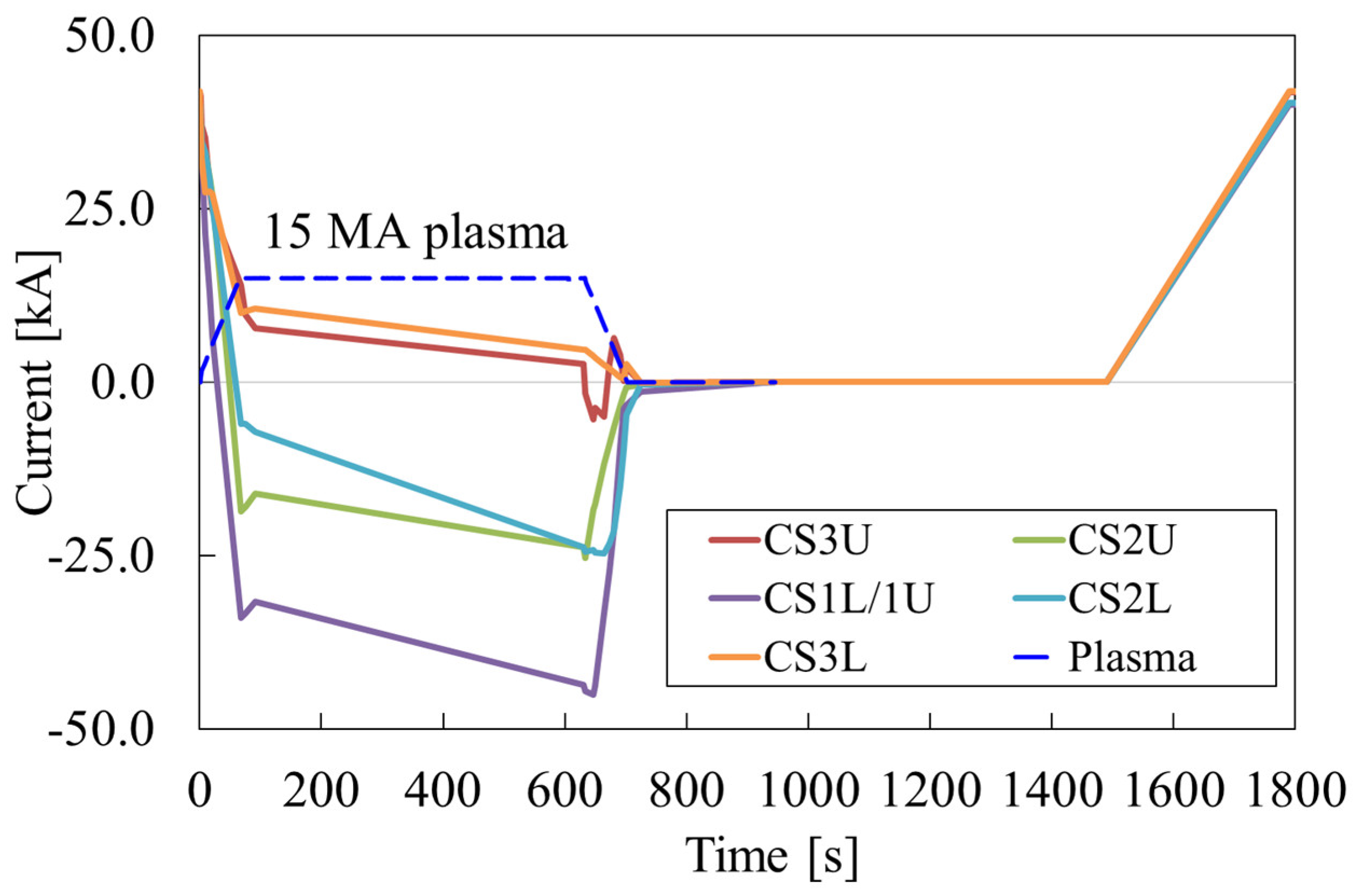
As shown in
Figure 7, the currents in the modules exhibit a rapid variation from +42 kA to −45 kA in less than 80 s. This fast current variation induces losses in the CS modules. In
Figure 8, the distribution of the losses in the CS modules is shown in some of the most relevant time instants during the plasma scenario. At the start of the plasma discharge, corresponding to
t = 0 s and
t = 1800 s, a peak in the losses can be observed at the inner turns of modules CS1L and CS1U, with the highest peak in module CS3L.
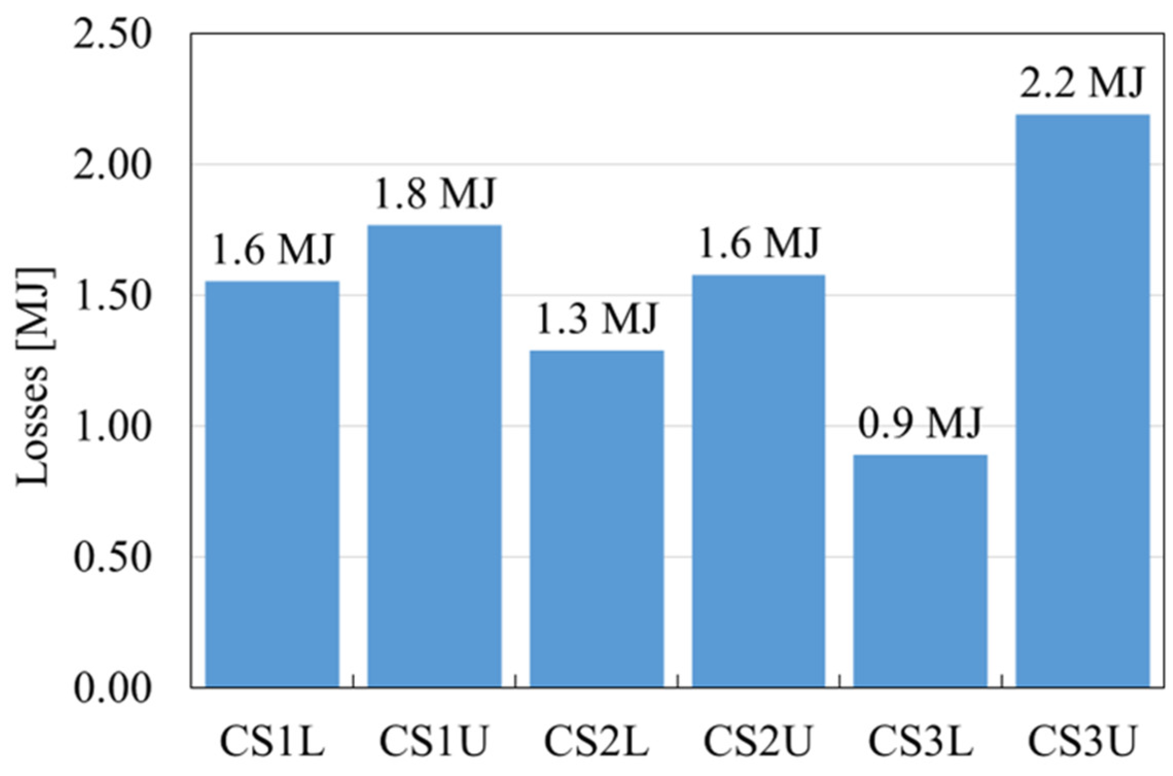
Despite the peak in losses during the plasma discharge, module CS3L has the smallest total amount of energy deposited during the plasma scenario, namely 0.9 MJ. The largest amount of 2.2 MJ is estimated for module CS3U. The total energy deposited in each module is shown in
Figure 9.
4.3. AC Losses in the Joints
The joints in the CS magnet are located at different positions and are subjected to different magnetic fields, as shown in
Figure 3b. The losses in the joints, retrieved from [
47] according to their location, are assumed constant during the scenario. The higher contributions are due to the coaxial and MB joints, with peak power of 5.95 W in the coaxial joint of module CS1L and 17.37 W in the MB joints of module CS1U. The losses in the splice joints and in the twin-box joints are much lower, below 0.22 W in both cases.
5. Result and Discussion
In this section, the hydraulic and thermal behaviours of the CS components—i.e., the pipes, cryogenic pump, winding pack and joints—are analysed during the 15 MA plasma scenario.
5.1. Performance of the Conductor During the Plasma Scenario
5.1.1. Temperature Evolution in the Pancakes
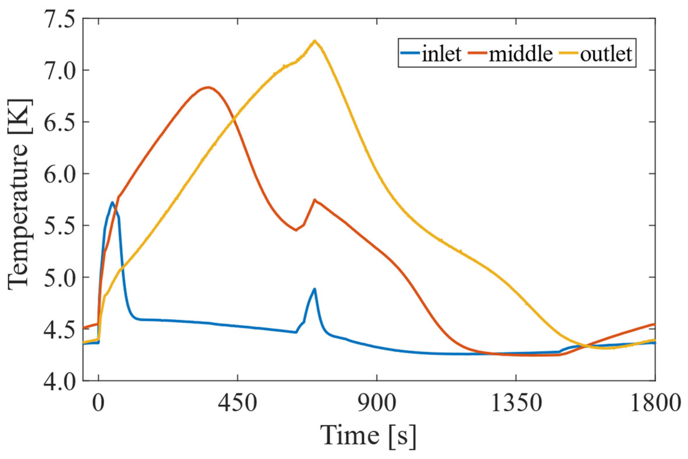
The temperature evolution in the bundle of the CICC is shown in
Figure 10 for pancake #39 of module CS1U. Three locations are selected, corresponding to the inlet (
x = 0 m), the middle point (
x = 73.75 m) and the outlet (
x = 147.5 m) section of the pancake. This pancake exhibits a peak temperature (7.4 K) at the outlet with respect to the other pancakes.
The temperature profile at the middle point of the pancake exhibits a peak at t = 300 s, while this peak is observed after about 6 min at the outlet. This delay is the transient time necessary for the helium in the conductor to flow along half of the pancake, corresponding to about 15 min to run through the 147.5-m-long pancake.
A further temperature increase is observed between 700 s and 1100 s in the middle point. This secondary temperature rise, although less pronounced than the major one, is related to the increase in losses corresponding to the end of plasma.
It is worth noting that, despite the amount of losses deposited in the inner turns of the modules, the cold circulator is able to maintain fresh helium at the inlet. A limited temperature increase (below 5.8 K) is observed at the inlet section of the pancake. After a transient of about 30 s, the temperature at the inlet is re-established at about 4.5 K.
The ability of the system to sustain stable temperature conditions at the inlet, and to efficiently dissipate the thermal load along the pancake, ensures robust performance under the nominal working conditions of the CS.
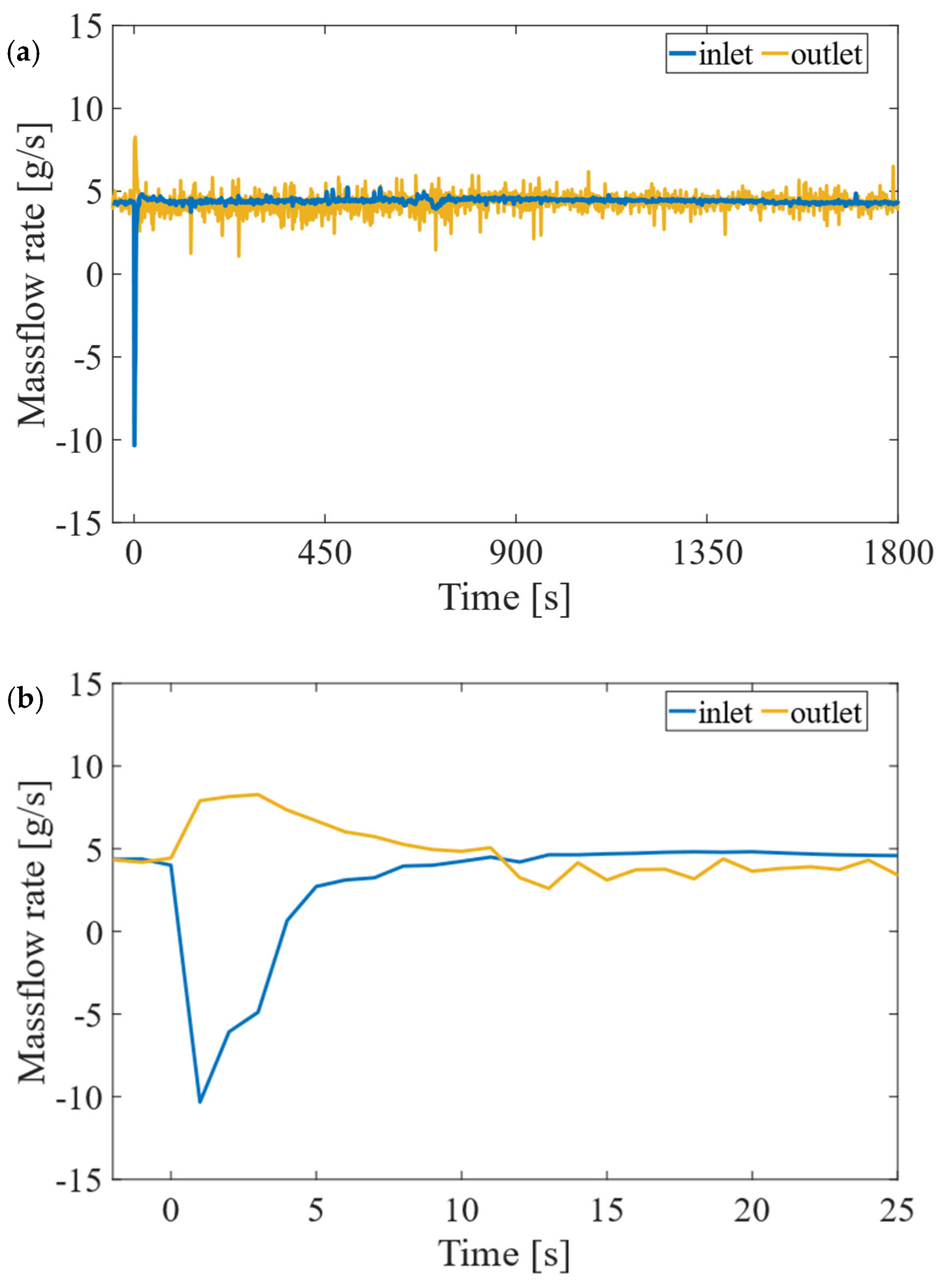
5.1.2. Mass Flow Rate Evolution in the Pancakes
Between
t = 0 s and
t = 10 s, helium backflow is observed at the inlets of modules CS3L, CS1L and CS1U. The reverse flow—which is not observed in the other modules—is due to the higher loss deposition in these modules than in the others during the start of the plasma discharge (
t = 0 s); see
Figure 8a.
An example is shown in
Figure 11a for the mass flow rate in the spiral of pancake #2, module CS3L. This module has the highest losses at
t = 0 s. An insight into the mass flow rate profile until
t = 25 s is shown in
Figure 11b. After a transient time of about 10 s, the circulator is able to re-establish the nominal flow with a mass flow rate of about 5 g/s in the spiral. This backflow, despite being undesired, does not have a remarkable impact on the performance of the conductor, as shown by the temperature increase discussed in the previous paragraph.
During the scenario, the mass flow rate in the bundle of the modules manufactured with KAT strands, i.e., CS2L and CS3U, is 16% higher than in the modules with JAS and FUR strands, i.e., CS3L, CS1L, CS1U and CS2U. The modules manufactured with KAT strands are in fact characterised by a lower friction factor than those manufactured with JAS and FUR strands.
In the modules manufactured with KAT strands, a portion corresponding to 52% of the helium flows in the spiral, while 48% flows in the bundle. In the modules with JAS and FUR strands, the flow repartition is slightly different, with 56% in the spiral and 44% in the bundle.
5.1.3. Pressure Evolution and Pressure Drop in the Pancakes
The pressure evolution in the spiral of the CICC during the scenario is shown in
Figure 12 for pancake #20 of module CS3U. Similar profiles, without any remarkable difference, are found for the other modules. The pressure drop of the pancakes during the scenario is between 0.65 bar and 0.48 bar.
The pressure dynamics observed during the scenario are directly influenced by the thermal inputs. As shown in
Figure 12, a fast pressure rise in the entire loop, above 3 bar, is observed between the SOD (
t = 0 s) and
t = 50 s. After this transient, the nominal flow is re-established, with a pressure of between 8 and 9 bar. A further fast pressure rise is observed between
t = 650 s and
t = 710 s. This further pressure rise of about 0.6 bar, smaller than the major one, is related to the loss rise corresponding to the end of the plasma.
5.2. Temperature Margin in the Conductor During the Plasma Scenario
The temperature margin (
) is computed as the difference between the temperature in the conductor (
) and the current-sharing temperature (
) at the same location and time instant (Equation (6)). Consequently, it depends on the value of the current in the module and on the magnetic flux density distribution.
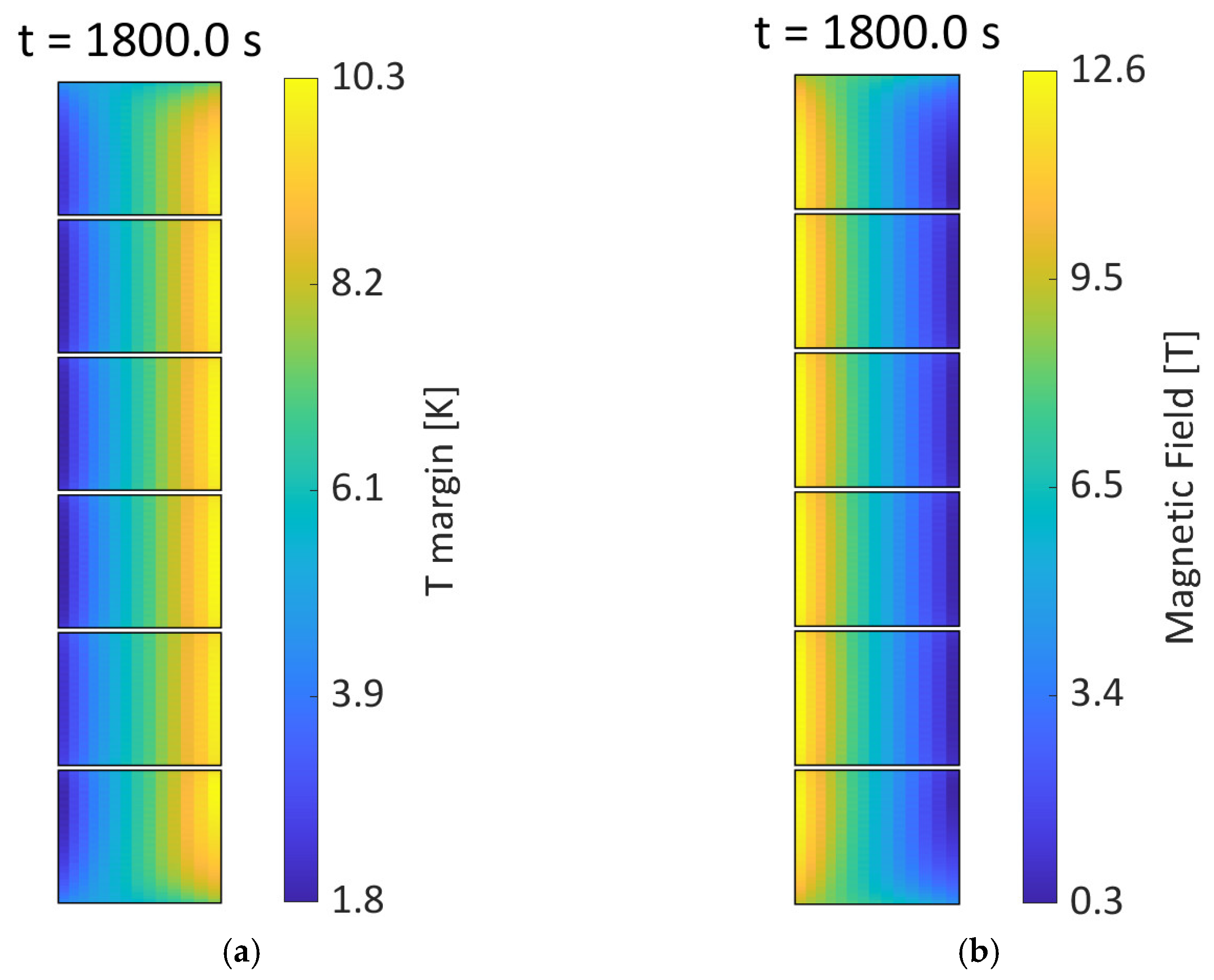
The minimum of the temperature margin is observed at the end of the plasma pulse, i.e.,
t = 1800 s. In
Figure 13a, the distribution of the temperature margin at the end of the pulse is shown. The inner turns, particularly turn #1, exhibit a lower margin. These turns are characterised by the highest magnetic flux density values, as shown in
Figure 13b.
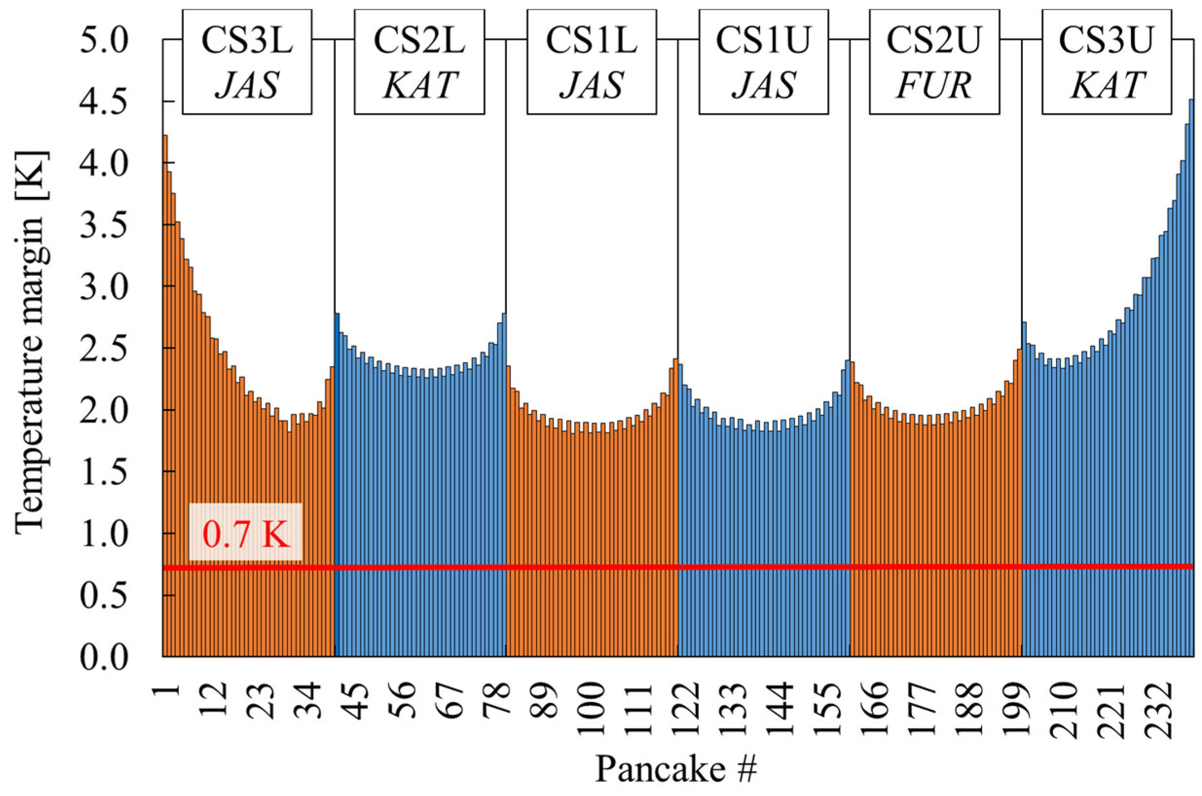
The minimum values of the temperature margin at the end of the pulse in each pancake of the module are shown in
Figure 14. These values, slightly below 2.0 K, are located in the central pancakes of the modules.
The minimum margins of 1.79 K for module CS1L and 1.82 K for module CS1U are found at x = 8.03 m, corresponding to 0.4 m from the outlet section of turn #1. The lowest value of 1.79 K fulfils the requirement of a temperature margin above 0.7 K.
5.3. Temperature in the Stack During the Plasma Scenario
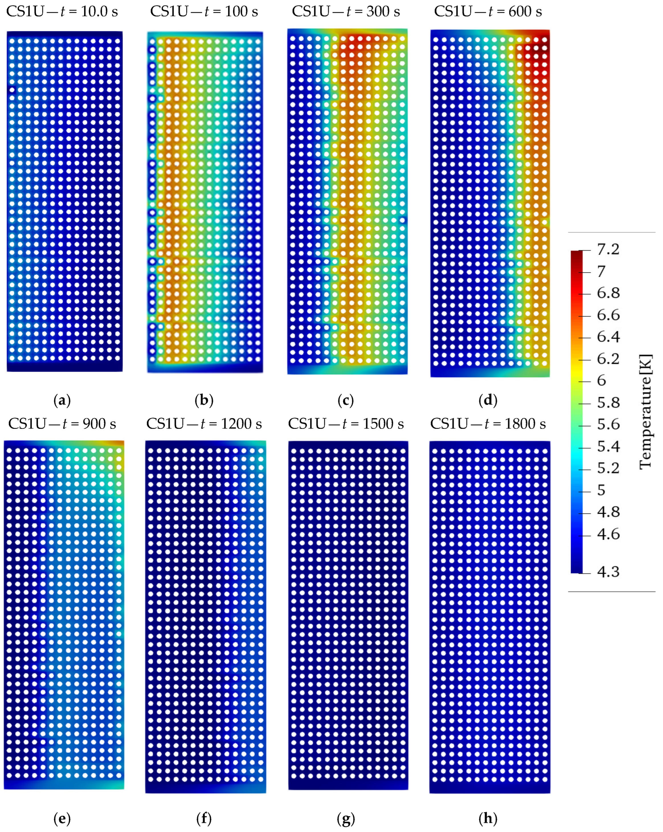
The temperature in the stack (the jacket of the cable and the inter-turn and inter-pancake insulation layers) during the plasma scenario in module CS1U is shown in
Figure 15. This module is selected as it exhibits the lowest temperature margin and also the temperature hotspot of the stack.
The heat deposited in the winding pack during the plasma scenario is removed by the fresh helium entering the pancakes. As an example, at
t = 100 s, turn #1 of every pancake is kept to a temperature lower than the others by the cold helium. At
t = 300 s, the central part of the stack exhibits the highest temperature, while, at
t = 900 s, the outer turns are the hottest ones. The hottest zone moves from the inner part (left part in
Figure 15) to the outer one (right part in
Figure 15). During the dwell, at
t = 1200.0 s, no remarkable hotspot zones are observed in the stack.
5.4. Performance of the Main Cryogenic Loop During the Plasma Scenario
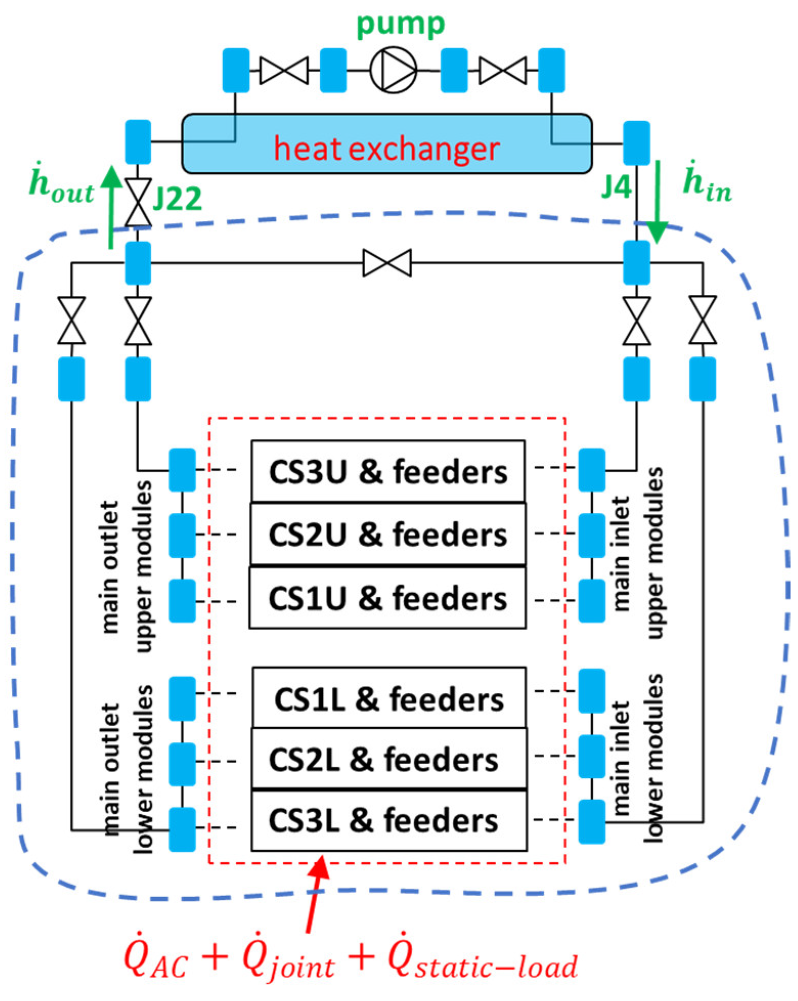
This section presents the behaviour of the main cryogenic loop, corresponding to the main inlet and outlet manifolds of the upper and lower modules (see
Figure 3).
5.4.1. Temperature in the Main Inlet/Outlet Pipes
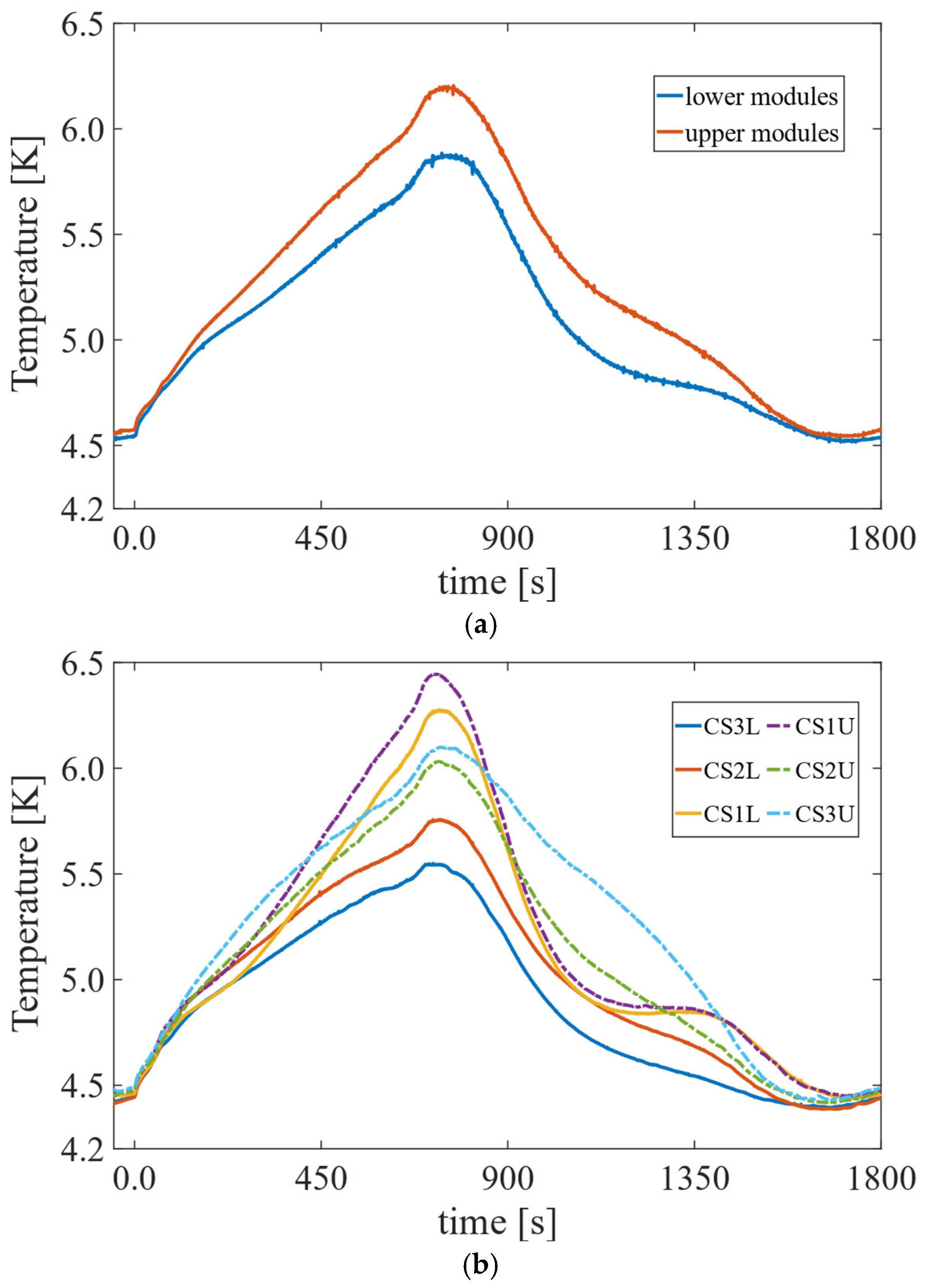
The temperatures of the two cooling pipes collecting the flow from the upper modules and from the lower modules are compared in
Figure 16a. Due to the different loss profiles, the outlet temperatures of the upper modules (CS3U, 2U and 1U) reach up to 0.4 K higher values than those of the lower modules (CS3L, 2L, 1L). The upper modules exhibit a peak temperature of 6.2 K, while 5.8 K is found at the same instant as in the lower modules. In
Figure 16b, the outlet temperatures of the six modules are compared.
5.4.2. Work of the Cryogenic Pump
The work of the pump can be computed by the enthalpy variation across the pump, i.e., the variation between its inlet and the outlet section:
where
is the mass flow rate;
and
are the pressure and temperature at the outlet;
is the corresponding enthalpy;
and
are the pressure and temperature at the inlet; and
is the corresponding enthalpy.
The total amount of energy required from the pump during the plasma scenario is computed by integrating Equation (5). In total, work amounting to about 2.4 MJ is required by the cryogenic pump to maintain nominal flow operation during one plasma pulse.
5.4.3. Heat Inventory of the CS System
The energy balance of the CS system during the plasma scenario is computed while accounting for the enthalpy variation of the helium between the inlet and outlet of the CS magnet (see the scheme in
Figure 17) and for the heat entering the magnet from the various sources, i.e., AC losses (
), joint losses (
) and the static heat load (
)):
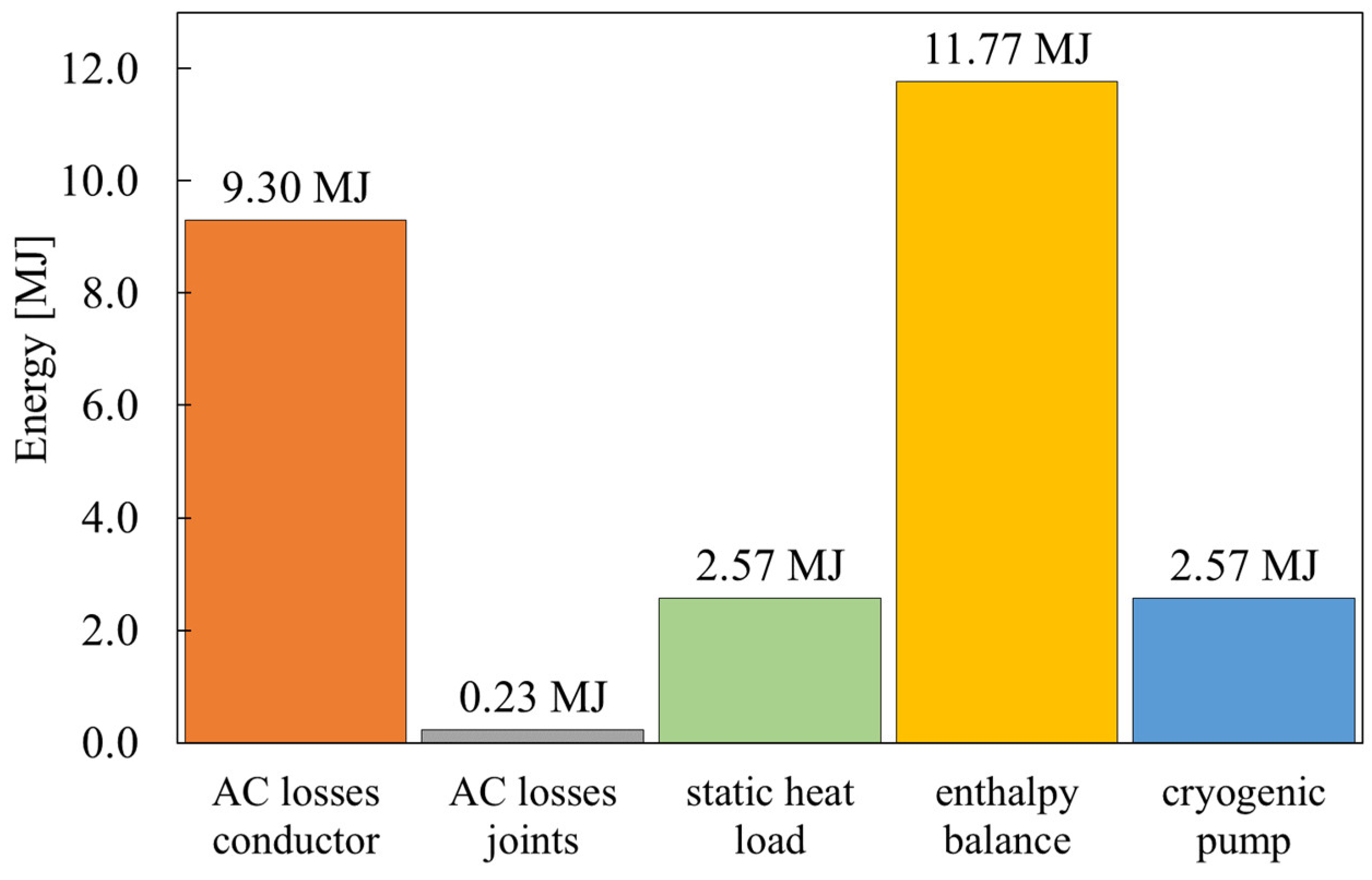
The total amount of energy computed by integrating the right-hand side of Equation (6) from t = 0 s to t = 1800 s gives 11.7 MJ.
During the scenario, a total amount of 9.3 MJ enters the CS magnet due to losses in the electrodynamic transient, while a smaller amount, about 0.23 MJ, is deposited in the joints. A total energy amount of 2.6 MJ enters the CS system due to the static heat load in the module supply and return lines and in the main busbars. Summing these contributions gives a total amount of about 12.1 MJ entering the system, which should be compared to the enthalpy variation of 11.7 MJ. The 3% difference between these two quantities can be ascribed to numerical errors. The aforementioned energy contributions are reported in the bar plot in
Figure 18.
6. Conclusions
The analysis of the ITER central solenoid during the 15 MA scenario was completed with a multi-physics model developed in the framework of the SuperMagnet suite of codes. This model reproduces the performance during the plasma scenario of the CS modules, namely six modules for a total of 240 pancakes, and of the cryogenic system, including about 4 km of pipes with about 30 valves, the circulator and the heat exchanger.
The main sources of losses that involve the CS and its cryogenic system during the scenario are accounted for in the model. A total amount of 12.1 MJ enters the system, and 75% of this total is attributed to AC losses and coupling and hysteresis losses, induced by the rapidly time-varying magnetic flux density and currents in the conductor. The static heat load in the feeders, arising from radiation heating from the thermal shields and conduction from the mechanical support, constitutes approximately 20% of the total losses. The losses in the joints are less than 1% of the total. The nuclear heating in the CS is almost negligible due the shielding effect of the components positioned between the plasma and the CS, such as the blanket, the vacuum vessel, the in-wall shielding, the thermal shield and the TF coils.
The model allows us to estimate the performance of the conductors during the plasma scenario. The temperature in the conductor exhibits a peak of 7.4 K in pancake #39 of module CS1U at t = 600 s. In the other modules, the peak temperature is below 7.0 K.
The larger amount of losses deposited at the inner turns of the CS determines a temperature increase, which is still limited to below 6.0 K, at the inlet of the pancakes. These higher losses also affect the flow circulation: a helium reverse flow is observed in particular in modules CS3L, CS1L and CS1U. After a transient time of about 10 s, the cryogenic pump is able to re-establish nominal flow operation, and fresh helium—with a temperature below 5 K—enters the pancakes without back flow during the remaining phases of the plasma scenario.
Analysing the results of the main cryogenic loop, a higher peak temperature is found at the manifold collecting the outlets of the upper modules (CS3U/2U/1U) than at the corresponding manifold of the lower modules (CS3L/2L/1L). This difference, still limited to about 0.4 K, is mainly due to the different loss profiles between the modules.
The main outcome of the model is the temperature margin of the coils during the plasma scenario, computed as the difference between the current-sharing temperature and the temperature in the conductor. A minimum value of 1.8 K is observed at the end of the plasma scenario in turn #1 of the central pancakes of modules CS3L, CS1L and CS1U, all assembled with Nb3Sn Jastec strands. This value is, in any case, above the prescribed threshold of 0.7 K for the CS conductor set by the design as the minimum margin.
Author Contributions
Conceptualization, L.C., M.B., J.L. and C.H.; methodology, L.C., M.B., J.L. and C.H.; software, L.C.; validation, L.C., M.B., J.L. and C.H.; formal analysis, L.C., M.B., J.L. and C.H.; investigation, L.C., M.B., J.L. and C.H.; resources, L.C., M.B., J.L. and C.H.; data curation, L.C., M.B., J.L. and C.H.; writing—original draft preparation, L.C.; writing—review and editing, L.C., M.B., J.L. and C.H.; visualization, L.C.; supervision, M.B. and C.H.; project administration, M.B. and C.H.; funding acquisition, M.B. and C.H. All authors have read and agreed to the published version of the manuscript.
Funding
The work at Università di Bologna was supported by the ITER Organization under contract # IO/20/CT/4300002342.
Institutional Review Board Statement
The views and opinions expressed herein do not necessarily reflect those of the ITER Organization.
Informed Consent Statement
Not applicable.
Data Availability Statement
The data presented in this study are available on request from the corresponding author. The data are not publicly available.
Acknowledgments
This paper is based on the work of many people. Particular mention to Florent Gauthier and Alexander Vostner of ITER Organization.
Conflicts of Interest
The authors declare no conflict of interest.
References
- ITER Physics Basis. Overview and summary. Nucl. Fusion 1999, 39, 2137–2174. [Google Scholar]
- A C C Sips, for the Steady State Operation and the Transport Physics Topical Groups of the International Tokamak Physics Activity. Advanced scenarios for ITER operation. Plasma Phys. Control. Fusion 2005, 47, A19–A40. [Google Scholar] [CrossRef]
- Wagner, F.; Becker, G.; Behringer, K.; Campbell, D.; Eberhagen, A.; Engelhardt, W.; Fussmann, G.; Gehre, O.; Gernhardt, J.; Gierke, G.V.; et al. Regime of Improved Confinement and High Beta in Neutral-Beam-Heated Divertor Discharges of the ASDEX Tokamak. Phys. Rev. Lett. 1982, 49, 1408. [Google Scholar]
- Schmitz, L. The role of turbulence–flow interactions in L- to H-mode transition dynamics: Recent progress. Nucl. Fusion 2017, 57, 025003. [Google Scholar] [CrossRef]
- Khayrutdinov, R.R.; Lukash, V.E. Studies of Plasma Equilibrium and Transport in a Tokamak Fusion Device with the Inverse-Variable Technique. J. Comp. Phys. 1993, 109, 193–201. [Google Scholar]
- Khayrutdinov, R.R.; Lister, J.B.; Lukash, V.E.; Wainwright, J.P. Comparing DINA code simulations with TCV experimental plasma equilibrium responses. Plasma Phys. Cont. Fusion 2001, 43, 321–342. [Google Scholar]
- Favez, J.-Y.; Khayrutdinov, R.R.; Lister, J.B.; Lukash, V.E. Comparing TCV experimental VDE responses with DINA code simulations. Plasma Phys. Cont. Fusion 2002, 44, 171–193. [Google Scholar]
- ITER Technical Basis. ITER EDA Documentation Series No. 24; IAEA: Vienna, Austria, 2002. [Google Scholar]
- Bauer, P.; Breschi, M.; Cavallucci, L.; Duchateau, J.L.; Gauthier, F.; Torre, A.; Turck, B. Description of the AC loss model for the ITER central solenoid during a plasma scenario. IEEE Trans. Appl. Supercond. 2022, 32, 4701305. [Google Scholar] [CrossRef]
- Torre, A.; Bauer, P.; Duchateau, J.L.; Gauthier, F.; Turck, B. Review of experimental results and models for AC losses in the ITER PF and CS conductors. IEEE Trans. Appl. Supercond. 2022, 32, 4700605. [Google Scholar]
- Cau, F.; Bessette, D.; Bauer, P.; Gauthier, F.; Portone, A.; Testoni, P.; Ventre, S. Update of Joule Losses Calculation in the ITER Cold Structures During Fast Plasma Transients. IEEE Trans. Appl. Supercond. 2020, 30, 4201404. [Google Scholar] [CrossRef]
- Albanese, R.; Rubinacci, G. Integral formulation for 3D eddy-current computation using edge elements. IEE Proc. A-Phys. Sci. Meas. Instrum. Manag. Educ.-Rev. 1988, 135, 457–462. [Google Scholar]
- Breschi, M.; Cavallucci, L.; Ribani, P.L.; Bauer, P. Electrodynamic Losses of the ITER PF Joints During the Dynamic Plasma Scenario. IEEE Trans. Appl. Supercond. 2023, 33, 4200705. [Google Scholar] [CrossRef]
- Breschi, M.; Cavallucci, L.; Adeagbo, H.; Sedlak, K.; Bajas, H.; Vostner, A.; Ilyin, Y. Performance review of the joints for the ITER poloidal field coils. Supercond. Sci. Technol. 2023, 36, 075009. [Google Scholar] [CrossRef]
- Fabbri, M.; Leichtle, D.; Martin, A.; Pampin, R.; Polunovskiy, E. Nuclear heat analysis for the ITER Vacuum Vessel regular sector. Fus. Eng. Des. 2018, 137, 435–439. [Google Scholar] [CrossRef]
- Wilson, M. Superconducting Magnets; Plenum Press: New York, NY, USA, 1983. [Google Scholar]
- Bottura, L. Modelling stability in superconducting cables. Phys. C 1998, 310, 316–326. [Google Scholar]
- Bottura, L. Thermal, Hydraulic, and Electromagnetic Modeling of Superconducting Magnet Systems. IEEE Trans. Appl. Supercond. 2016, 26, 4901807. [Google Scholar]
- Meyder, R. Investigation on effects of conductor concepts on 3D quench propagation in superconducting coils using the code system MAGS. J. Fusion Energy 1993, 12, 99–105. [Google Scholar]
- Bottura, L. SARUMAN—An integrated procedure for the analysis of quench in superconducting magnets. IEEE Trans. Magn. 1994, 30, 1978–1981. [Google Scholar]
- Bottura, L. A Numerical Model for the Simulation of Quench in the ITER Magnets. J. Comput. Phys. 1996, 125, 26–41. [Google Scholar]
- Gornikel, I.V.; Kalinin, V.V.; Kaparkova, M.V.; Kukhtin, V.P.; Shatil, D.N.; Shatil, N.A.; Sytchevsky, S.E.; Vasiliev, V.N. VENECIA: New Code for Simulation of Thermohydraulics in Complex Superconducting Systems. Math. Inf. Sci. Phys. 2010, 2, 127–131. [Google Scholar]
- Alphysica. Available online: http://www.alphysica.com/index.php/venecia.html (accessed on 1 March 2025).
- Richard, L.S.; Casella, F.; Fiori, B.; Zanino, R. The 4C code for the cryogenic circuit conductor and coil modeling in ITER. Cryogenics 2010, 50, 167–176. [Google Scholar]
- Bonifetto, R.; De Bastiani, M.; Di Zenobio, A.; Muzzi, L.; Turtu, S.; Zanino, R.; Zappatore, A. Analysis of the Thermal-HydraulicEffects of a Plasma Disruption on the DTT TF Magnets. IEEE Trans. Appl. Supercond. 2022, 32, 4204007. [Google Scholar]
- Gorit, Q.; Nicollet, S.; Lacroix, B.; Louzguiti, A.; Torre, A.; Topin, F.; Vallcorba, R.; Zani, L. JT-60SA TF coil quench model and Analysis: Joule energy estimation with SuperMagnet and STREAM. Cryogenics 2022, 124, 103454. [Google Scholar]
- Lee, H.; Oh, S.; Jung, L. Thermo-Hydraulic Analysis of the KSTAR PF Cryogenic Loop Using SUPERMAGNET Code. IEEE Trans. Appl. Supercond. 2022, 28, 4205505. [Google Scholar]
- CryoSoft, SuperMagnet, Multitasking Code Manager”, User’s Guide, Version 2.1, February 2016. Available online: https://supermagnet.sourceforge.io/supermagnet.html (accessed on 1 March 2025).
- Available online: https://htess.com/cryosoft/ (accessed on 1 March 2025).
- Bagnasco, M.; Bessette, D.; Bottura, L.; Marinucci, C.; Rosso, C. Progress in the Integrated Simulation of Thermal-Hydraulic Operation of the ITER Magnet System. IEEE Trans. Appl. Supercond. 2010, 20, 411–414. [Google Scholar] [CrossRef]
- Libeyre, P.; Mitchell, N.; Bessette, D.; Gribov, Y.; Jong, C.; Lyraud, C. Detailed design of the ITER central solenoid. Fus. Eng. Des. 2009, 84, 1188–1191. [Google Scholar] [CrossRef]
- Schultz, J.H.; Antaya, T.; Feng, J.; Gung, C.Y.; Martovetsky, N.; Minervini, J.V.; Michael, P.; Radovinsky, A.; Titus, P. The ITER Central Solenoid. In Proceedings of the 21st IEEE/NPS Symposium on Fusion Engineering SOFE 05, Knoxville, TN, USA, 26–29 September 2005; pp. 1–4. [Google Scholar] [CrossRef]
- Reiersen, W. (ITER Organization, St. Paul Lez Durance, France); DDD11-3: CS Coils and Pre-Compression Structure. IDM 2NHKHH 2013. 2013; (Unpublished work). [Google Scholar]
- Bauer, P. (ITER Organization, St. Paul Lez Durance, France); DDD11-6: Feeders, CTBs and Current Leads. IDM 2NMSYG 2011. 2011; (Unpublished work). [Google Scholar]
- CryoSoft, Flower, Hydraulic Network Simulation”, User’s Guide, version 4.5, January 2016. Available online: https://supermagnet.sourceforge.io/flower.html (accessed on 1 March 2025).
- Bottura, L.; Rosso, C. Flower, a model for the analysis of hydraulic networks and processes. Cryogenics 2003, 43, 215–223. [Google Scholar]
- Gauthier, F.; Bessette, D.; Oh, D.-K. Thermal Hydraulic Analysis of the ITER PF and Correction Coils in 15 MA Scenario Operation Using the SuperMagnet Suite of Codes. IEEE Trans. Appl. Supercond. 2014, 24, 4201705. [Google Scholar] [CrossRef]
- CryoSoft, Thea, Thermal, Hydraulic and Electrical Analysis of Superconducting Cables”, User’s Guide, Version 2.3, September 2016. Available online: https://supermagnet.sourceforge.io/thea.html (accessed on 1 March 2025).
- Bottura, L.; Rosso, C.; Breschi, M. A general model for thermal, hydraulic and electric analysis of superconducting cables. Cryogenics 2000, 40, 617–626. [Google Scholar]
- Bagni, T.; Duchateau, J.-L.; Breschi, M.; Devred, A.; Nijhuis, A. Analysis of ITER NbTi and Nb3Sn CICCs experimental minimum quench energy with JackPot, MCM and THEA models. Supercond. Sci. Technol. 2017, 30, 095003. [Google Scholar] [CrossRef]
- Bottura, L.; Bordini, B. Jc(B,T,ε) Parameterization for the ITER Nb3Sn Production. IEEE Trans. Appl. Supercond. 2009, 19, 1521–1524. [Google Scholar] [CrossRef]
- Katheder, H. Optimum thermohydraulic operation regime for cable in conduit superconductors (CICS). Cryogenics 1994, 34, 595–598. [Google Scholar] [CrossRef]
- Katheder, H. (The NET Team, Max Planck Institut für Plasmaphysik, Garching bei München, Germany); A General Formula For Calculation of the Friction Factor for Cable in Conduit Conductors. The NET Team, Internal Note N/R/0821/26/A 1993. 1993; (Unpublished work). [Google Scholar]
- Martovetsky, N.; Michael, P.; Minervini, J.; Radovinsky, A.; Takayasu, M.; Gung, C.; Thome, R.; Ando, T.; Isono, T.; Hamada, K.; et al. Test of the ITER central solenoid model coil and CS insert. IEEE Trans. Appl. Supercond. 2002, 12, 600–605. [Google Scholar] [CrossRef]
- Martovetsky, N.; Freudenberg, K.; Rossano, G.; Wooley, K.; Khumthong, K.; Norausky, N.; Ortiz, E.; Sheeron, J.; Smith, J.; Bonifetto, R.; et al. Testing of the ITER CS Module #4. IEEE Trans. Appl. Supercond. 2024, 34, 4200206. [Google Scholar] [CrossRef]
- Gauthier, F. (ITER Organization, St. Paul Lez Durance, France); et al.; Summary of Friction Factor Correlations for ITER Superconducting Magnet CICC. IDM 4GRMAX 2021. 2021; (Unpublished work). [Google Scholar]
- Bessette, D. (ITER Organization, St. Paul Lez Durance, France); CS Analysis During DINA2016-01 with the Venecia Model. Internal Report, IDM YDW582 v 1.0, March 2019. 2019; (Unpublished work). [Google Scholar]
- Martovetsky, N.; Isono, T.; Bessette, D.; Devred, A.; Nabara, Y.; Zanino, R.; Savoldi, L.; Bonifetto, R.; Bruzzone, P.; Breschi, M.; et al. Characterization of the ITER CS conductor and projection to the ITER CS performance. Fus. Eng. Des. 2017, 124, 1–5. [Google Scholar] [CrossRef]
- Breschi, M.; Bianchi, M.; Bonifetto, R.; Carli, S.; Devred, A.; Martovetsky, N.; Ribani, P.L.; Savoldi, L.; Takaaki, I.; Zanino, R. Analysis of AC Losses in the ITER Central Solenoid Insert Coil. IEEE Trans. Appl. Supercond. 2017, 27, 7762085. [Google Scholar]
- CryoSoft, Heater, Simulation of Heat Conduction”, User’s Guide, Version 2.1, February 2016. Available online: https://supermagnet.sourceforge.io/heater.html (accessed on 1 March 2025).
- Giarratano, P.J.; Arp, V.; Smith, R. Forced Convection Heat Transfer to Supercritical Helium. Cryogenics 1971, 11, 385–393. [Google Scholar]
- Gribov, Y. (ITER Organization, St. Paul Lez Durance, France); DINA Simulation of 15 MA DT Scenario: DINA 2016-01. IDM SFGRPW v 1.1. 2016; (Unpublished work). [Google Scholar]
- Bauer, P.; Breschi, M.; Cavallucci, L.; Duchateau, J.-L.; Gauthier, F.; Ilyin, Y.; Schild, T.; Torre, A.; Turck, B. AC Losses Calculations for the ITER CS and PF Magnet Systems during Plasma Operation. IEEE Trans. Appl. Supercond. 2023, 33, 1–5. [Google Scholar]
- Breschi, M.; Cavallucci, L.; Ribani, P.L.; Bonifetto, R.; Zappatore, A.; Zanino, R.; Gauthier, F.; Bauer, P.; Martovetsky, N. AC losses in the first ITER CS module tests: Experimental results and comparison to analytical models. IEEE Trans. Appl. Supercond. 2021, 31, 5900905. [Google Scholar]
- Breschi, M.; Cavallucci, L.; Bauer, P.; Gauthier, F.; Bonifetto, R.; Zappatore, A.; Zanino, R.; Martovetsky, N.; Khumthong, K.; Ortiz, E.; et al. AC Losses in the Second Module of the ITER Central Solenoid. IEEE Trans. Appl. Supercond. 2022, 32, 4700505. [Google Scholar]
- Breschi, M.; Cavallucci, L.; Ribani, P.L.; Gauthier, F. AC Loss Modeling of a Full-Size ITER CS Module. IEEE Trans. Appl. Supercond. 2023, 33, 5900212. [Google Scholar]
- Gauthier, F. (ITER Organization, St. Paul Lez Durance, France); SuperMagnet Model Update Of ACB#1 (PBS34.3C) CS (PBS11.CS) Under 15 MA DT Plasma Scenario (Baseline 2008). IDM 4RH5YE v 1.1, February 2021. 2021; (Unpublished work). [Google Scholar]
Figure 1.
(
a) CS modules [
33,
34]; (
b) CS feeder system [
33,
34].
Figure 1.
(
a) CS modules [
33,
34]; (
b) CS feeder system [
33,
34].
Figure 2.
Conductor cross-section: (a) CS, (b) busbar lead extension and (c) MB.
Figure 2.
Conductor cross-section: (a) CS, (b) busbar lead extension and (c) MB.
Figure 3.
(a) Hydraulic scheme of the cryogenic system and (b) module feeder and joint locations. The filled blue squares represent manifolds. The other filled squares represent different types, namely the coaxial, twin-box, MB and splice joints (see the legend).
Figure 3.
(a) Hydraulic scheme of the cryogenic system and (b) module feeder and joint locations. The filled blue squares represent manifolds. The other filled squares represent different types, namely the coaxial, twin-box, MB and splice joints (see the legend).
Figure 4.
Sketch of the Thea CICCs in one CS module.
Figure 4.
Sketch of the Thea CICCs in one CS module.
Figure 5.
Friction factor as a function of the flow regime in the bundle and spiral of the CICCs manufactured with KAT, JAS and FUR strands.
Figure 5.
Friction factor as a function of the flow regime in the bundle and spiral of the CICCs manufactured with KAT, JAS and FUR strands.
Figure 6.
Two-dimensional mesh of the nine stacks in Heater.
Figure 6.
Two-dimensional mesh of the nine stacks in Heater.
Figure 7.
Current profile in the CS modules during the plasma scenario.
Figure 7.
Current profile in the CS modules during the plasma scenario.
Figure 8.
AC losses in the CS during some of the relevant instants of the plasma scenario: (a) t = 0 s, start of discharge; (b) t = 70 s, start of current flattop; (c) t = 500 s, end of burn; (d) t = 704.5 s, end of plasma; (e) t = 1790 s, end of rebias; (f) t = 1800 s, start of discharge.
Figure 8.
AC losses in the CS during some of the relevant instants of the plasma scenario: (a) t = 0 s, start of discharge; (b) t = 70 s, start of current flattop; (c) t = 500 s, end of burn; (d) t = 704.5 s, end of plasma; (e) t = 1790 s, end of rebias; (f) t = 1800 s, start of discharge.
Figure 9.
Total energy deposited in the modules by the AC losses during the plasma scenario.
Figure 9.
Total energy deposited in the modules by the AC losses during the plasma scenario.
Figure 10.
Temperature of the bundle in pancake #39, module CS1U, at the inlet (x = 0.0 m), middle point (x = 73.75 m) and outlet (x = 147.5 m).
Figure 10.
Temperature of the bundle in pancake #39, module CS1U, at the inlet (x = 0.0 m), middle point (x = 73.75 m) and outlet (x = 147.5 m).
Figure 11.
Mass flow rate in the spiral at the inlet, middle point and outlet of (a) pancake #2, module CS3L; (b) insight into helium backflow until t = 25 s.
Figure 11.
Mass flow rate in the spiral at the inlet, middle point and outlet of (a) pancake #2, module CS3L; (b) insight into helium backflow until t = 25 s.
Figure 12.
Pressure profile in the spiral at the inlet, middle point and outlet of pancake #20, module CS3U.
Figure 12.
Pressure profile in the spiral at the inlet, middle point and outlet of pancake #20, module CS3U.
Figure 13.
(a) Temperature margin and (b) magnetic flux density in the CS at the end of the pulse, t = 1800 s.
Figure 13.
(a) Temperature margin and (b) magnetic flux density in the CS at the end of the pulse, t = 1800 s.
Figure 14.
Minimum value of the temperature margin over the pancakes of the CS at the end of the pulse, t = 1800 s.
Figure 14.
Minimum value of the temperature margin over the pancakes of the CS at the end of the pulse, t = 1800 s.
Figure 15.
Temperature profile in the stack of module CS1U at (a) t = 10 s; (b) t = 100 s; (c) t = 300 s; (d) t = 600 s; (e) t = 900 s; (f) t = 1200 s; (g) t = 1500 s; (h) t = 1800 s.
Figure 15.
Temperature profile in the stack of module CS1U at (a) t = 10 s; (b) t = 100 s; (c) t = 300 s; (d) t = 600 s; (e) t = 900 s; (f) t = 1200 s; (g) t = 1500 s; (h) t = 1800 s.
Figure 16.
Temperature profile during the scenario: (a) main outlet pipes of lower and upper modules; (b) outlet of each module.
Figure 16.
Temperature profile during the scenario: (a) main outlet pipes of lower and upper modules; (b) outlet of each module.
Figure 17.
Scheme of the enthalpy balance.
Figure 17.
Scheme of the enthalpy balance.
Figure 18.
Energy balance of the CS and the cryogenic circuit during the plasma scenario.
Figure 18.
Energy balance of the CS and the cryogenic circuit during the plasma scenario.
Table 1.
Conductor strand manufacturers.
Table 1.
Conductor strand manufacturers.
| CS Module | Strand Type | Manufacturer |
|---|
| CS3U | Nb3Sn
(internal tin) | Kiswire Advanced
Technology (KAT) |
| CS2U | Nb3Sn
(bronze) | Furukawa
(FUR) |
| CS1U | Nb3Sn
(bronze) | Jastec
(JAS) |
| CS1L | Nb3Sn
(bronze) | Jastec
(JAS) |
| CS2L | Nb3Sn
(internal tin) | Kiswire Advanced
Technology (KAT) |
| CS3L | Nb3Sn
(bronze) | Jastec
(JAS) |
busbar
lead extension (EXT) | Nb3Sn
(bronze) | Jastec
(JAS) |
main busbar
(MB) | NbTi | Western Superconducting
Technologies (WST) |
Table 2.
Friction factor parameters for the bundle and the spiral.
Table 2.
Friction factor parameters for the bundle and the spiral.
| |
(Bundle) |
(Bundle) |
(Bundle) |
(Bundle) |
(Spiral) |
(Spiral) |
|---|
| JAS | −0.742 | 19.5 | 0.0487 | 0.855 | 0.0492 | 0.0 |
| FUR | −0.742 | 19.5 | 0.0487 | 0.855 | 0.0492 | 0.0 |
| KAT | −0.742 | 19.5 | 0.0291 | 0.886 | 0.0842 | 0.0 |
| MB | −0.742 | 19.5 | 0.0231 | 0.7953 | / | / |
Table 3.
Parameters of the strain model.
Table 3.
Parameters of the strain model.
| | | | |
|---|
| JAS | −0.60942% | −1.0777 × 10⁻⁹ [A/T] | 0.0% |
| FUR | −0.66826% | −3.555 × 10⁻¹⁰ [A/T] | 0.0% |
| KAT | −0.57576% | −1.6263 × 10⁻⁹ [A/T] | 0.0% |
Table 4.
Plasma scenario.
Table 4.
Plasma scenario.
| Start of Discharge (SOD) | 0.0 s | End of Cooling (EOC) | 600.102 s |
| End of Plasma Initiation | 1.346 s | End of Plasma | 704.502 s |
| X Point Formation (XPF) | 11.502 s | Start of Dwell | 975 s |
| Start of Current Flattop (SOF) | 70.102 s | End of Dwell | 1490 s |
| Start of Burn (SOB) | 90.502 s | End of Rebias | 1790 s |
| End of Burn (EOB) | 500.102 s | SOD | 1800 s |
| Start of Discharge (SOD) | 0.0 s | End of Cooling (EOC) | 600.102 s |
| End of Plasma Initiation | 1.346 s | End of Plasma | 704.502 s |
| Disclaimer/Publisher’s Note: The statements, opinions and data contained in all publications are solely those of the individual author(s) and contributor(s) and not of MDPI and/or the editor(s). MDPI and/or the editor(s) disclaim responsibility for any injury to people or property resulting from any ideas, methods, instructions or products referred to in the content. |
© 2025 by the authors. Licensee MDPI, Basel, Switzerland. This article is an open access article distributed under the terms and conditions of the Creative Commons Attribution (CC BY) license (https://creativecommons.org/licenses/by/4.0/).


