Fault Diagnosis of Wind Turbine Blades Based on One-Dimensional Convolutional Neural Network-Bidirectional Long Short-Term Memory-Adaptive Boosting and Multi-Source Data Fusion

Abstract

To prevent wind turbine blade accidents and improve fault detection accuracy, a hybrid deep learning model based on 1D CNN-BiLSTM-AdaBoost for wind turbine-blade fault classification is proposed. Fault data are first preprocessed by segmenting and labeling the fault patterns. Features are extracted through the convolutional layers, followed by dimensionality reduction and denoising using the pooling layers, and feature fusion. The multi-source sensor features are then fed into the BiLSTM layer for further processing of the time-series characteristics. The processed data are classified through a fully connected layer. Finally, multiple weak classifiers are combined to generate the final classification result. Experimental results show that the 1D CNN-BiLSTM-AdaBoost model outperforms models that use only 1D CNN, BiLSTM, and 1D CNN-BiLSTM, achieving an accuracy of 96.88%, precision of 97.22%, recall of 96.92%, and an F1 score of 96.86%, with a maximum accuracy of 100%. These results validate the model’s effectiveness for fault classification.

1. Introduction

Wind energy has emerged as an efficient and sustainable power source, gaining widespread adoption in recent years. Wind turbine blades are critical components of wind energy systems, and early detection of faults is essential to ensure their reliability and prevent costly repairs [1]. Common faults in wind turbines include fractures, deformations, and vibration issues, which can significantly impact performance and safety. These faults often manifest as subtle changes in sensor data, making their detection challenging [2,3].

Traditional fault detection methods primarily rely on manual inspections and single-sensor diagnostic techniques, such as vibration, temperature, and pressure analysis. However, these approaches exhibit several limitations. Manual inspections are inherently subjective, inefficient, and prone to misjudgments [4]. Single-sensor-based methods are susceptible to environmental noise and signal interference, making it challenging to comprehensively assess turbine conditions. Additionally, conventional signal processing techniques often struggle to capture subtle fault-related features and long-term dynamic variations in complex operating environments, thereby limiting diagnostic accuracy [5].

With the rapid advances in sensor technology and data processing capabilities, multi-sensor data fusion has emerged as a promising approach for fault diagnosis. Liu et al. [6] demonstrated that integrating multi-sensor features significantly enhances bearing fault detection accuracy. Similarly, Chao et al. [7] employed multi-source sensor data, including vibration and pressure signals, to achieve precise fault diagnosis in reciprocating pumps through feature fusion techniques. Deep learning, particularly in the context of multi-sensor data fusion and temporal sequence modeling, has further revolutionized fault detection. Convolutional neural networks (CNNs), long short-term memory (LSTM) networks, and their variants, such as BiLSTM, have been extensively applied to fault mode recognition and health monitoring [8,9]. Among these models, one-dimensional CNNs (1D-CNNs) have been widely adopted for processing time-series data due to their ability to automatically extract local features, capture short-term dependencies, and reduce preprocessing requirements [10]. However, 1D-CNNs exhibit limitations in capturing long-term dependencies and global dynamic patterns, which may lead to critical information loss in certain fault signals, thereby affecting diagnostic performance.

To address these shortcomings, this study integrates LSTM networks with 1D-CNNs. LSTM’s superior memory capabilities enable the effective capture of long-term dependencies within time-series data, complementing 1D-CNN’s local feature extraction. By combining 1D-CNN and LSTM, the proposed model preserves the sensitivity of CNN to local patterns while simultaneously leveraging LSTM’s ability to model long-range temporal dependencies. This hybrid approach significantly enhances fault diagnosis accuracy and robustness [11]. For instance, Wang et al. demonstrated the effectiveness of 1D-CNN in fusing multimodal bearing sensor signals while incorporating visualization techniques to analyze model behavior [12]. Eren et al. utilized 1D-CNNs for the real-time processing of large-scale bearing datasets, revealing superior performance compared to other deep learning models [13]. Additionally, Chen et al. proposed a 1D-CNN architecture incorporating progressively reduced convolutional kernel sizes and dropout operations, achieving a diagnostic accuracy of 98% on public bearing datasets [14]. Furthermore, Huang et al. developed a hybrid CNN-LSTM model, demonstrating high recognition accuracy even under noisy conditions [15], while Shi et al. introduced a CNN-BiLSTM framework for extracting integrated vibration and rotational speed features, effectively diagnosing gearbox faults in varying operational conditions [16]. Despite the significant advancements achieved through CNN-LSTM integration, practical deployment remains challenging due to data complexity, noise interference, and imbalanced fault sample distributions. To overcome these challenges, ensemble learning techniques have been introduced to enhance diagnostic performance. Adaptive boosting (AdaBoost), a widely used ensemble learning algorithm, iteratively trains multiple weak classifiers while assigning higher weights to misclassified samples, thereby constructing a robust classifier [17]. This approach effectively mitigates the impact of noise and outliers while improving classification performance under imbalanced sample distributions. For example, Guo et al. [18] applied a reinforced AdaBoost model to wind turbine-blade ice fault detection, while An et al. [19] combined AdaBoost with extreme learning machines to enhance wind power prediction accuracy. In this study, AdaBoost is incorporated into the CNN-LSTM hybrid model to leverage the advantages of multiple weak classifiers, further improving fault feature recognition and enhancing system robustness. This integration not only reduces misclassification rates but also ensures high diagnostic precision under variable operating conditions.

This study aims to develop a deep learning-based fault diagnosis model by integrating 1D-CNN and LSTM networks while incorporating AdaBoost for ensemble optimization. The 1D-CNN extracts local temporal features and fuses multi-sensor data, BiLSTM captures bidirectional temporal dependencies and global information, and AdaBoost enhances the overall model performance. This approach addresses the limitations of conventional fault diagnosis methods, significantly improving the accuracy, real-time responsiveness, and robustness of wind turbine-blade fault detection. The findings not only provide theoretical and technical support for wind turbine fault diagnosis but also offer valuable insights for the design of intelligent monitoring and maintenance systems in practical engineering applications.

The remainder of this paper is structured as follows: Section 2 details the design of the integrated model, Section 3 describes the wind turbine-blade fault dataset and diagnostic model training, Section 4 presents experimental validation, and Section 5 concludes with general findings and future research directions.

2. Designed 1D CNN-BiLSTM-AdaBoost Model

2.1. Model Overview

The proposed model integrates dual-channel fault features and utilizes the AdaBoost algorithm to optimize performance. During the preprocessing stage, the fault data are segmented, and fault labels are printed. Feature extraction is then performed through convolutional layers, followed by dimensionality reduction and denoising via pooling layers. To mitigate the risk of overfitting, a dropout layer is incorporated after certain convolutional layers. Subsequently, the features from different channels are fused at the feature layer and passed into the BiLSTM layer for further processing of temporal features. After passing through the fully connected layer, the extracted features are used for classification. Finally, the AdaBoost algorithm combines multiple weak classifiers through a weighted ensemble to generate the final classification result. The process is illustrated in Figure 1.

2.2. Detailed Model Description

2.2.1. Design of the 1D CNN

The core components of the 1D CNN include convolutional layers, pooling layers, flattening layers, and fully connected layers [20]. The basic principle is illustrated in Figure 2. In the figure, T represents the length of the input data time window, and $V$ denotes the number of variables across all sampled points. The convolution kernel $f$ slides across a specific dimension of the time domain to extract dynamic features, enabling the extraction of high-level abstract feature representations from each convolutional layer. The feature $h_j^l\in R^{c_{1\times 1}}$ can be expressed as follows:

$${\mathrm{h}}_j^l=\sigma ({\mathrm{H}}^{l-1}\ast {\mathrm{f}}_j^{\prime }+{\mathrm{b}}_j^i)$$

(1)

where $h_j^l$ refers to the $j_{th}$ feature at the $l_{th}$ layer; $H^{l-1}=\left[h_1^{l-1},h_2^{l-1},\cdots ,h_N^{l-1}\right]\in R^{C_{l-1}\times N_{l-1}}$ represents the $l-1_{th}$ convolutional layer; $f_j^l$ is the $j_{th}$ convolution kernel at the $l_{th}$ layer; $b_j^l$ represents the network bias; $C$ is the feature dimension; $N$ indicates the number of convolution kernels; $\sigma (·)$ is the nonlinear activation function; and $*$ denotes the convolution operation.

The 1D CNN layer is adjusted through multiple iterations, ultimately selecting three different convolution kernel sizes (the convolutional layer group consists of three convolutional layers). The convolutional layers use ReLU as the activation function. The pooling layer reduces the input data size while retaining essential feature information, using max pooling. The dropout layer is employed to mitigate overfitting of neurons. Through experimentation, the dropout probability is set to 0.5.

The flattening layer transforms the local features from the three convolutional layers into a single vector by merging and integrating all relevant elements. These features are then passed to the BiLSTM model and subsequently to the fully connected layer for further processing.

2.2.2. Data Fusion

Sensor fusion refers to the integration and optimization of data collected from multiple sensors of the same or different types, positioned at different spatial locations. It is generally categorized into the following three types: data-level fusion, feature-level fusion, and decision-level fusion [21].

Data-level fusion involves directly concatenating raw sensor data [22]. Feature-level fusion is an intermediate approach where features are first extracted from the raw data and then integrated [23]. Decision-level fusion first derives decision-related information from the data before integrating the individual decisions [24]. A comparative analysis of the advantages and disadvantages of these three fusion strategies is presented in

Table 1. Comparison of data fusion methods.

Fusion Type	Advantages	Disadvantages
Data-level fusion	Provides rich information with high accuracy	Requires handling different data formats and precision
Feature-level fusion	Combines features from different sensors, enhancing robustness and efficiency	Effective feature extraction and selection can be complex
Decision-level fusion	Allows independent decision-making by each sensor, offering flexibility	More complex; decision-making at the sensor level is challenging

.

Compared to data-level and decision-level fusion, feature-level fusion is a more mature approach. It reduces the complexity of input data, avoids information redundancy, and preserves both local and global information, thereby enhancing accuracy and robustness. Additionally, it is more flexible as it does not require additional model training. Feature-level fusion effectively leverages deep learning models’ feature learning capabilities, further improving model performance. Therefore, this study adopts feature-level fusion for data processing.

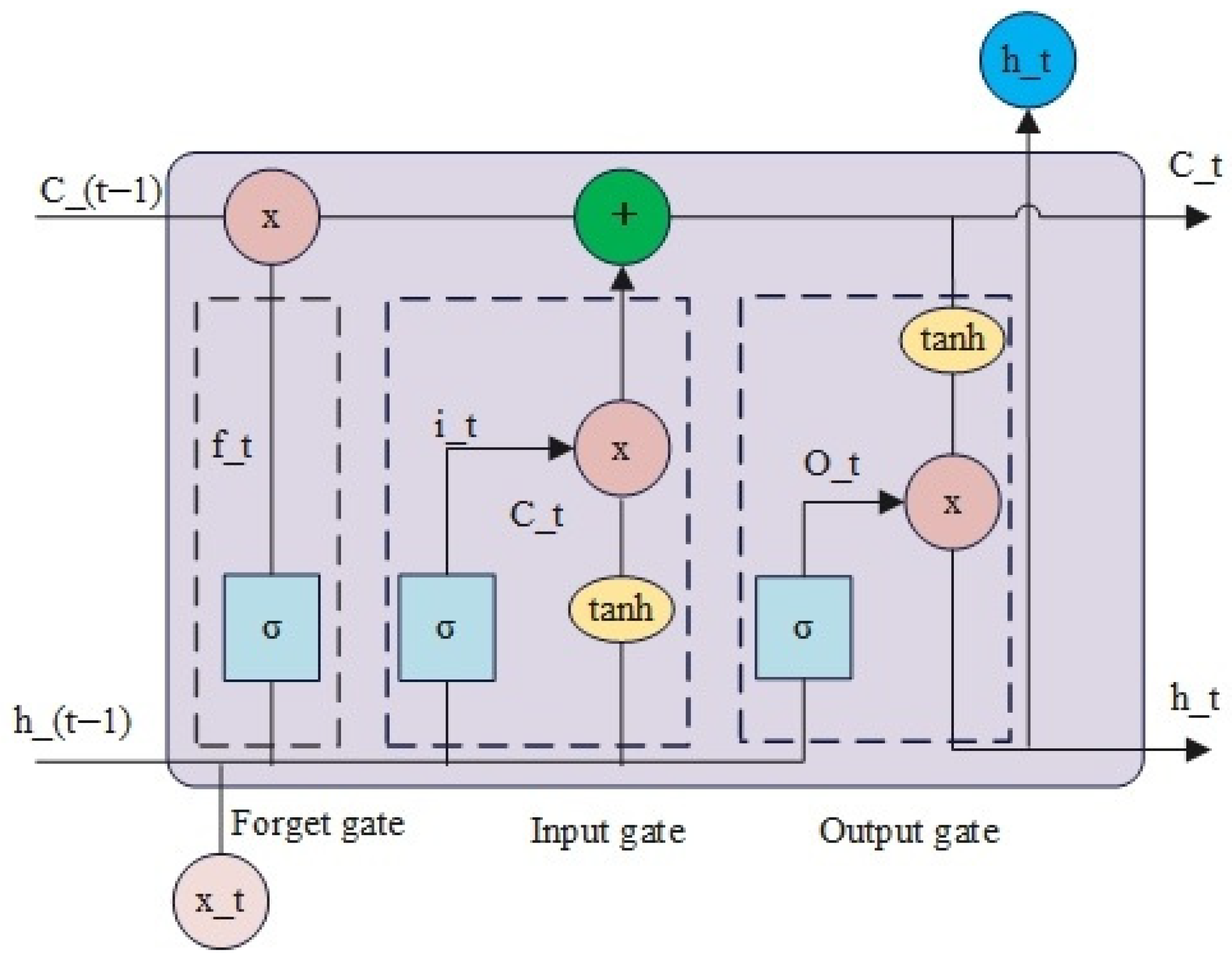
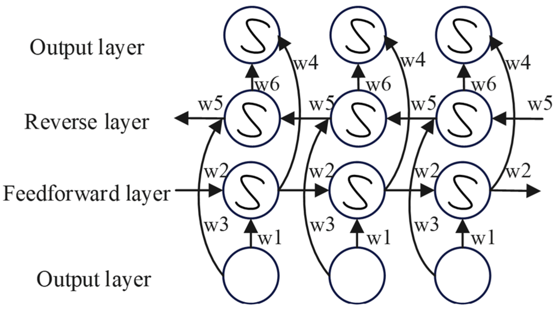
2.2.3. BiLSTM Architecture

BiLSTM is a variant of LSTM. Unlike conventional LSTM, which can only utilize past time-series data for predictions, BiLSTM incorporates both forward and backward LSTM layers, enabling more comprehensive information processing. The fundamental principle of LSTM is illustrated in Figure 3.

In a BiLSTM model, two independent LSTMs operate in parallel: a forward LSTM and a backward LSTM, which is presented in Figure 4.

Forward LSTM: Processes the input sequence ${\mathrm{x}}_1,{\mathrm{x}}_2,\dots ,{\mathrm{x}}_{\mathrm{T}}$ sequentially from time step $\mathrm{t}=1$ to $\mathrm{t}=\mathrm{T}$.

$${\overrightarrow{h}}_t={\mathrm{LSTM}}_{\mathrm{forward}}\left(x_t,{\overrightarrow{h}}_{t-1}\right)$$

(2)

Backward LSTM: Processes the input sequence ${\mathrm{x}}_{\mathrm{T}},{\mathrm{x}}_{\mathrm{T}-1},\dots ,{\mathrm{x}}_1$ in reverse order sequentially from time step $\mathrm{t}=\mathrm{T}$ to $\mathrm{t}=1$.

$${\overleftarrow{h}}_t={\mathrm{LSTM}}_{\mathrm{backward}}\left(x_t,{\overleftarrow{h}}_{t+1}\right)$$

(3)

Bidirectional Hidden State: At each time step, the hidden state of the BiLSTM is formed by concatenating the hidden states of the forward and backward LSTMs:

$$h_t=\left[{\overrightarrow{h}}_t;{\overleftarrow{h}}_t\right]$$

(4)

where $\overrightarrow{h}$ represents the hidden state of the forward LSTM at time step t; $\overleftarrow{h}$ is the hidden state derived from the backward LSTM; and $h_t$ is the final hidden state at time step t, obtained by concatenating the forward and backward hidden states.

The final output of the BiLSTM is typically computed by mapping the bidirectional hidden states at each time step ${\mathrm{h}}_{\mathrm{t}}$ to the desired output dimension through a linear layer:

$$y_t=W_y·h_t+b_y$$

(5)

where $W_y$ is the weight matrix and $b_y$ is the bias term.

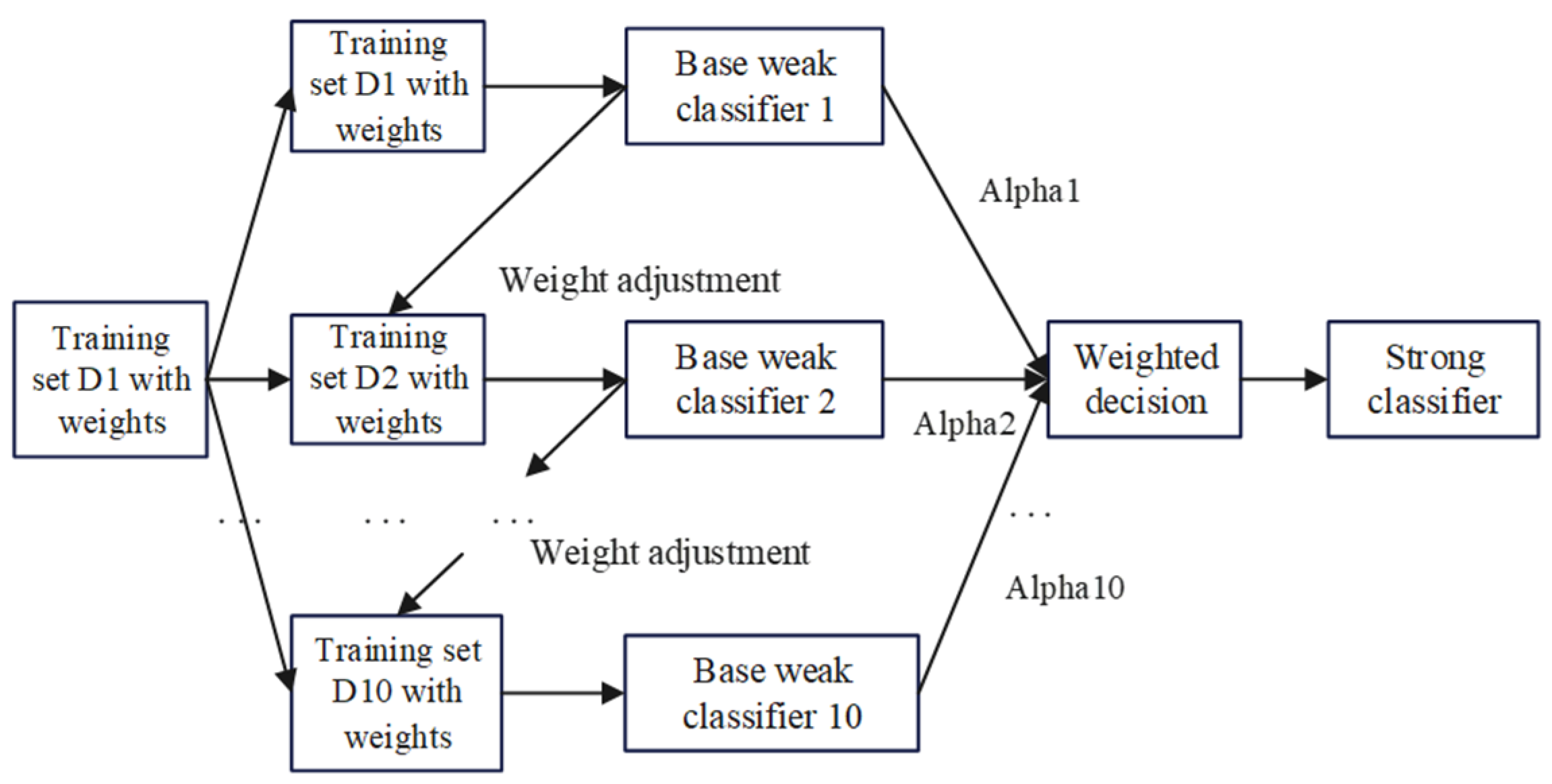
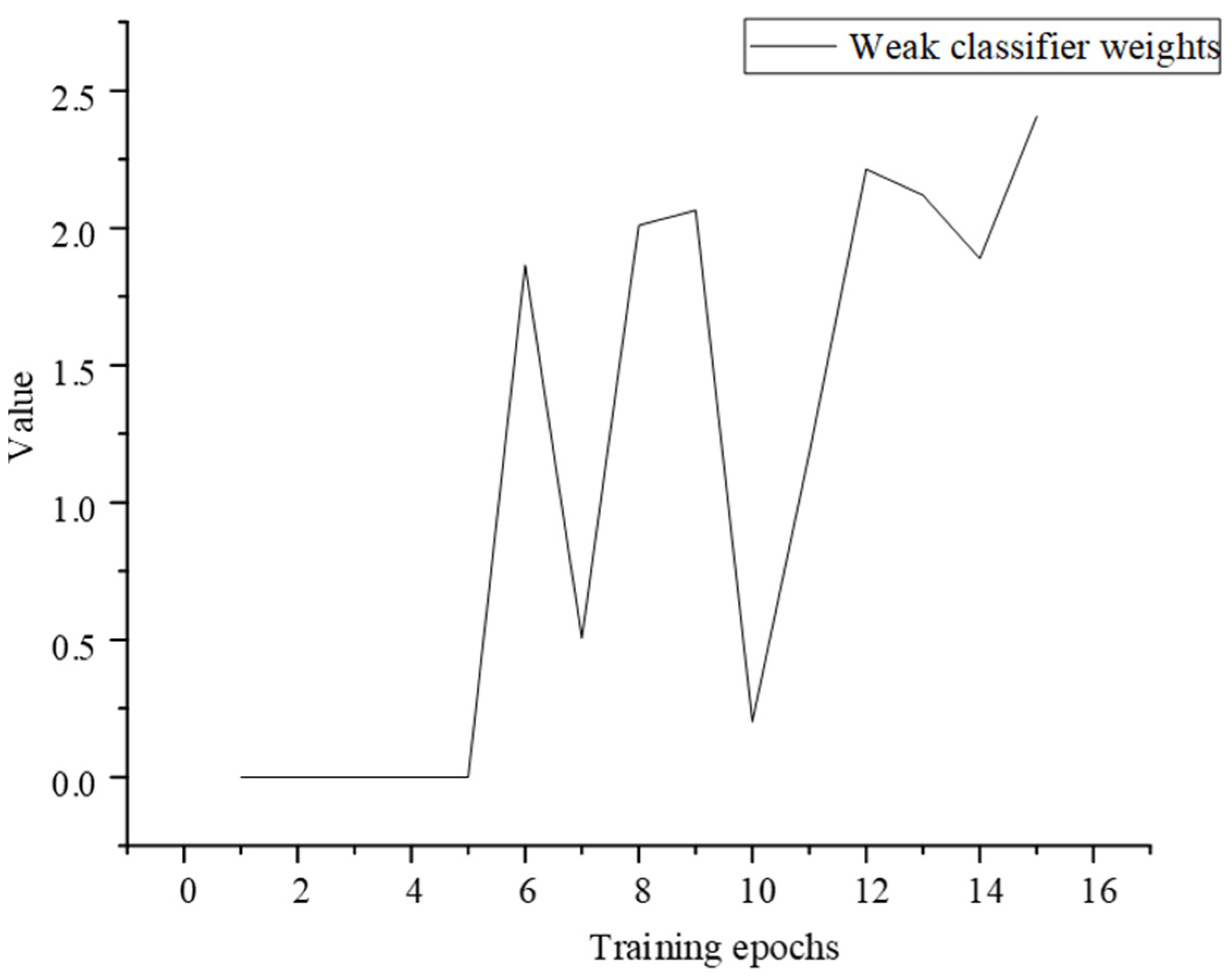
2.2.4. AdaBoost Network Architecture

The AdaBoost algorithm employs a 1D CNN-BiLSTM as a weak classifier. The fundamental principle of the algorithm is illustrated in Figure 5.

The algorithm consists of three main steps:

(1) Initialization of Data Weight Distribution

The initial weight distribution of the training samples is defined as follows:

$$D_i=\left(w_1,w_2,\dots w_N\right)=\left({\displaystyle \frac{1}{N}},\dots \dots ·{\displaystyle \frac{1}{N}}\right)$$

(6)

where $D_i$ represents the initial weight distribution; $w_i$ denotes the weight of the $i$ sample; and $N$ represents the total number of samples.

(2) Iterative Selection of Weak Classifiers

The AdaBoost algorithm iteratively selects weak classifiers over multiple rounds, where t = 1, 2…, T represents the iteration step.

① Selection of the weak classifier. The weak classifier $\mathrm{h}$ with the lowest error rate in the current round is selected as the $\mathrm{t}$-th base classifier ${\mathrm{H}}_{\mathrm{t}}$. The classification error ${\mathrm{e}}_{\mathrm{t}}$ on the weight distribution ${\mathrm{D}}_{\mathrm{t}}$ is computed as follows:

$$e_t=P\left(H_t\left(x_i\ne y_i\right)\right)={\displaystyle \sum _{i=1}^N{w}_{ti}}I\left(H_t\left(x_i\right)\ne y_i\right)$$

(7)

where $I\left(H_t\left(x_i\right)\ne y_i\right)$ is an indicator function that takes a value of 1 when $H_t\left(x_i\right)$ makes an incorrect prediction and 0 otherwise and $\mathrm{i}$ denotes the index of the sample $N$.

② Computation of the classifier’s weight. The coefficient $H_t\left(x\right)$ of the weak classifier in this iteration is calculated, representing its weight in the final ensemble classifier.

$$a_t={\displaystyle \frac{1}{2}}\ln \left({\displaystyle \frac{1-e_t}{e_t}}\right)$$

(8)

③ Weight adjustment for the next iteration. The weight distribution of the training dataset is updated to guide the subsequent iteration. The weight adjustment formula is as follows:

$$D_{t+1}={\displaystyle \frac{D_t(i)\exp \left(-a_t{y}_i{H}_t\left(x_i\right)\right)}{z_t}}$$

(9)

where $D_t(i)$ is the weight of the $i$-th sample in the $t$-th iteration; $y_i$ represents the ground truth label; $H_t\left(x_i\right)$ represents the prediction result of the $t$-th weak classifier; and $Z_t$ is the normalization constant $Z_t=2\sqrt{e_t\left(1-e_t\right)}$.

(3) Formation of the final strong classifier

The algorithm of AdaBoost-1DCNN-BiLSTM is presented in Algorithm 1. After multiple iterations, the weak classifiers ${\mathrm{H}}_{\mathrm{t}}\left(\mathrm{x}\right)$ and their corresponding weights are combined to form a strong classifier using the sign function:

$$f(x)={\displaystyle \sum _{t-1}^T{a}_t}{H}_t(x)$$

(10)

The final classifier is obtained through the application of the sign function sign, as follows:

$$H_{\mathrm{final}}=\mathrm{sign}(f(x))=\mathrm{sign}\left({\displaystyle \sum _{t-1}^T{a}_t}{H}_t(x)\right)$$

(11)

Algorithm 1: AdaBoost-1DCNN-BiLSTM
Input: Training dataset ${\left\{(x_i,y_i)\right\}}_{i=1}^N$, weak classifier 1DCNN-BiLSTM, number of iterations T
Output: Final strong classifier f(x)
1. Initialize the weight distribution
	Assign an initial weight to each training sample $x_i(i=1,2,\dots ,N)$ according to Equation (6).
2. Iterative training of weak classifiers
	For t = 1, 2, …, T, perform the following steps:
	① Train the weak classifier and compute the error rate Train the weak classifier $D_t$ using 1DCNN-BiLSTMbased on the current weight distribution $h_t$; Compute the classification error rate on $D_t$ using Equation (9).
	② Compute the weight of the weak classifier
	Determine the weight coefficient of $h_t$ in the final ensemble model using Equation (10).
	③ Update the weight distribution of training samples
	Update the weight of each sample according to Equation (11) to guide the next iteration.
3. Construct the strong classifier
	① Combine all weak classifiers and their corresponding weights using Equation (12);
	② Obtain the final strong classifier f(x) through Equation (13).

3. Wind Turbine Blade Fault Dataset and Fault Diagnosis Model Training

3.1. Data Collection

The dataset used in this study was obtained from the ZENODO platform, originating from the Institute of Structural Engineering at ETH Zurich. It consists of fault data for small wind turbine blades. R (healthy state): Normal operating condition. C (simulated icing fault): A mass block (3 × 44 g) is added to simulate an icing fault. H and L (crack faults): Cracks are introduced at 17%, 30%, and 50% of the blade’s longitudinal axis. Each crack has the following three variations: length 5 cm, 10 cm, or 15 cm. Depth and width: 4 mm and 1.5 mm, respectively. Cracks are set at different positions and lengths to simulate various crack fault scenarios. A summary of the fault settings is presented in

Table 2. Fault setting overview.

Label	Description
R	Healthy state
C	Mass block added (3 × 44 g) to simulate icing fault
H	Crack $l_1$= 10 cm, Crack $l_2$= 10 cm, Crack $l_3$= 5 cm
L	Crack $l_1$= 15 cm, Crack $l_2$= 15 cm, Crack $l_3$= 15 cm

. The training process is presented in Figure 6.

Experimental tests were conducted under controlled conditions: C-type faults were detected using S22 and S17 sensors. H- and L-type faults, along with the R (healthy) state, were monitored using A2 and S9-1 sensors. All data were collected at a stable temperature of 25 °C, with white noise used as the excitation source. For each fault condition, 50,000 data samples were collected; 15,000 samples were allocated for testing. The remaining samples were used for training.

3.2. Model Fault Training

The 1DCNN-BiLSTM-AdaBoost algorithm is trained on a computer with Windows 10, Intel (R) Core (TM) i7-8750H CPU @ 2.20GHz2.21GHz, and NVIDIA GTX 1060 GPU with a video memory capacity of 10 GB. It is developed in the Python (version 3.9.19) language deep learning framework system PyTorch (version 2.0.0+cu118).

The main training steps of the 1DCNN-BiLSTM-AdaBoost model are as follows:

(1) Input the two-way fault data required for 1DCNN-BiLSTM-AdaBoost training;

(2) Initialize the parameters of each network, such as the number of convolutional layers, the size of the hidden layer of BiLSTM, the number of weak classifiers, the weight of each weak classifier, etc.;

(3) Train the basic weak classifier 1DCNN-BiLSTM model, extract features from the fault data through 1DCNN and perform feature fusion and then pass it to BiLSTM for further feature extraction;

(4) Determine whether all weak classifiers have been calculated. If no, adjust the weights of each classifier and continue training; if yes, output the strong classifier results according to the weights of each classifier.

3.3. Model Hyperparameter Setting

Hyperparameter setting in deep learning is an important part of optimizing model performance. The performance of the AdaBoost weak classifier directly affects the performance of the final strong classifier. Too many BiLSTM neurons will cause the model to overfit, and too few will cause the model’s performance to deteriorate. Keeping the input size unchanged, the loss function obtained by changing the number of neurons is shown in Figure 7. Observing Figure 7a, when the number of neurons is set to 128, although the training set has good convergence, the test set has an overfitting problem; increasing the number of neurons to 256 as shown in Figure 7b, the overfitting problem of the test set is more serious; reducing the number of neurons to 32 as shown in Figure 7c, it is found that the overfitting problem of the test set has improved a little, but the loss function value remains in a larger range, and the convergence speed is slow; further increasing the number of neurons to 64 as shown in Figure 7d, it is found that the overfitting problem of the test set has also been well handled, and the loss function value can be maintained in a smaller range. After adjustment, the BiLSTM network input size is set to 64, including 2 hidden layers, each with 64 neurons. The parameters of the model after adjustment are shown in

Table 3. Hyperparameter settings.

Hyperparameter	Value
Learning rate	0.00002
Batch_size	8
Number of training rounds	500
Number of convolution kernels	1408
Number of convolution kernels	32, 3, 5, 7
Number of BiLSTM neurons	64
Number of BiLSTM layers	2
Activation function	ReLU
Optimizer	AdamW
Drop_out	0.5
Loss function	Cross entropy
Number of weak classifiers	10

.

4. Model Verification and Comparison Based on 1DCNN-BiLSTM-AdaBoost

4.1. Evaluation Indicators

In this study, the model’s performance is comprehensively evaluated using metrics such as the confusion matrix, cross-entropy loss function, precision, accuracy, recall, and F1-score. These metrics are widely used in deep learning and pattern recognition, as they not only reflect the model’s convergence during training but also provide a multifaceted assessment of its effectiveness in real-world fault detection tasks. For instance, the cross-entropy loss function measures the discrepancy between the predicted probability distribution and the true labels, while the confusion matrix visually represents the model’s classification performance across different categories. The following section will provide a detailed explanation of each evaluation metric, including their definitions and computation formulas, followed by an in-depth discussion of the experimental results in subsequent chapters.

4.1.1. Confusion Matrix

The confusion matrix is a tool for measuring the performance of the category model. For the actual label set $y_{\mathrm{true}}$ and the predicted label set $y_{\mathrm{pred}}$, the elements of the confusion matrix C are calculated as follows:

$$C_{i,j}={\displaystyle \sum _{k=1}^N\delta }\left(y_{\mathrm{true}}^{(k)},i\right)·\delta \left(y_{\mathrm{pred}}^{(k)},j\right)$$

(12)

where $N$ is the total number of test samples; $y_{\mathrm{true}}^{(k)}$ is the true category of the $k$-th sample; $y_{\mathrm{pred}}^{(k)}$ is the predicted category of the $k$-th sample; and $\delta (a,b)$ is the Kronecker delta function, which takes the value 1 when $\mathrm{a}=\mathrm{b}$, otherwise it is 0.

4.1.2. Loss Function

This paper uses the cross entropy loss function to evaluate the model, which combines the Softmax function and the negative log-likelihood loss and calculates the difference between the prediction result and the actual label by the model.

$$\mathrm{Loss}=-{\displaystyle \frac{1}{N}}{\displaystyle \sum _{i=0}^{N-1}{\displaystyle \sum _{k=0}^{K-1}{y}_{i,k}}}\ln p_{i,k}$$

(13)

where $y_{i,k}$ indicates that the true label of the $i$-th sample is $k$, there are $K$ label values and $N$ samples, and $p_{i,k}$ indicates the probability that the $i$-th sample is predicted to be the $k$-th label value.

4.1.3. Indicators

The formulas of four indicators are presented as follows.

$$\mathrm{Accuracy}={\displaystyle \frac{\mathrm{TP}+\mathrm{TN}}{\mathrm{TP}+\mathrm{FP}+\mathrm{FN}+\mathrm{TN}}}$$

(14)

$$\mathrm{Precision}={\displaystyle \frac{\mathrm{TP}}{\mathrm{TP}+\mathrm{FP}}}$$

(15)

$$\mathrm{Recall}={\displaystyle \frac{\mathrm{TP}}{\mathrm{TP}+\mathrm{FN}}}$$

(16)

$$\mathrm{Fmeasure}={\displaystyle \frac{1}{\frac{1}{\mathrm{Precision}}+\frac{1}{\mathrm{Recall}}}}$$

(17)

The formula introduction is shown in

Table 4. Meaning of the formula.

Real Situation	Prediction Result
	Prediction Value = True Class	Prediction Value = False Class
True value = true class	TP (true class)	FN (false negative class)
True value = false class	FP (false positive class)	TN (true negative class)

.

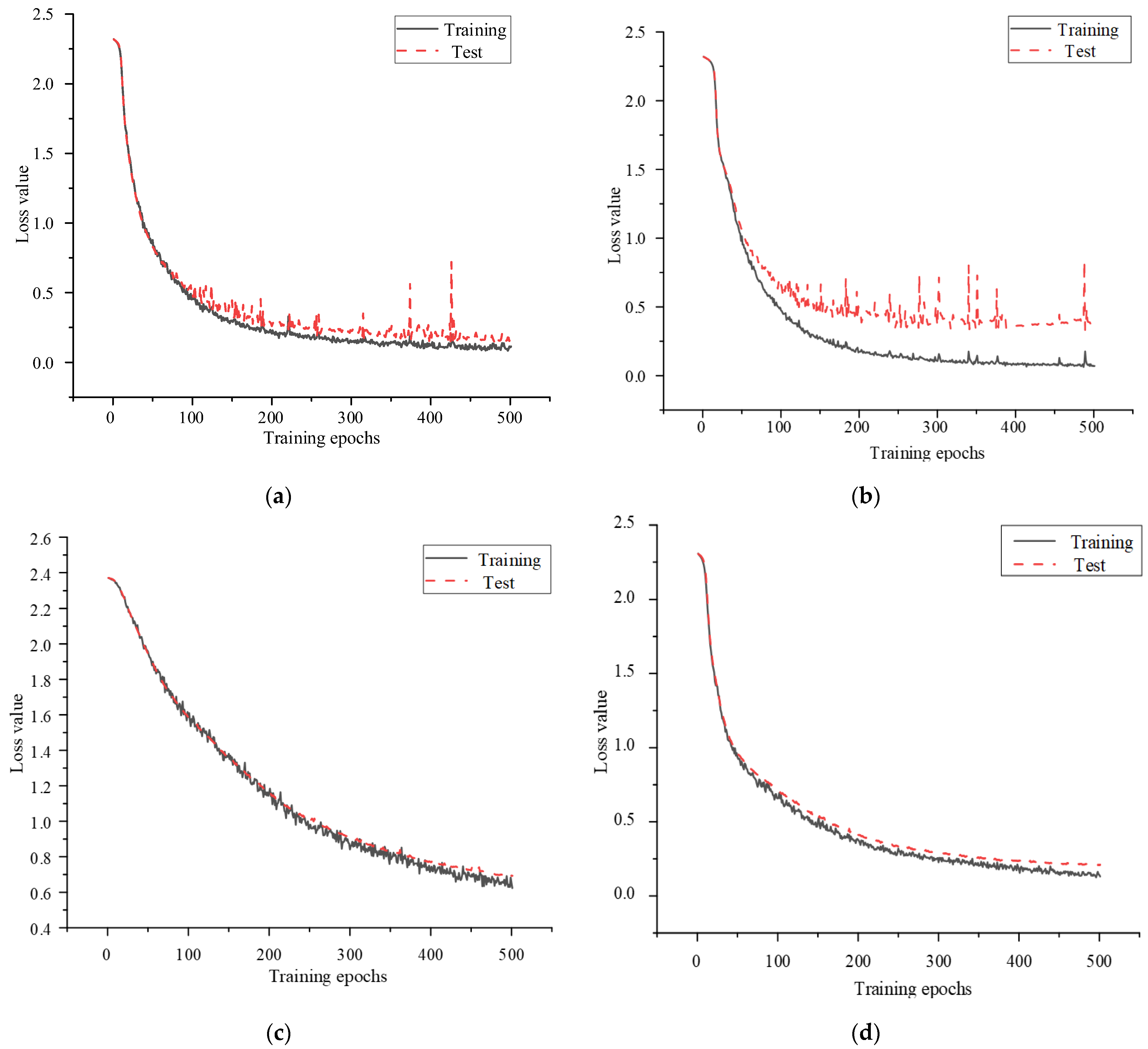
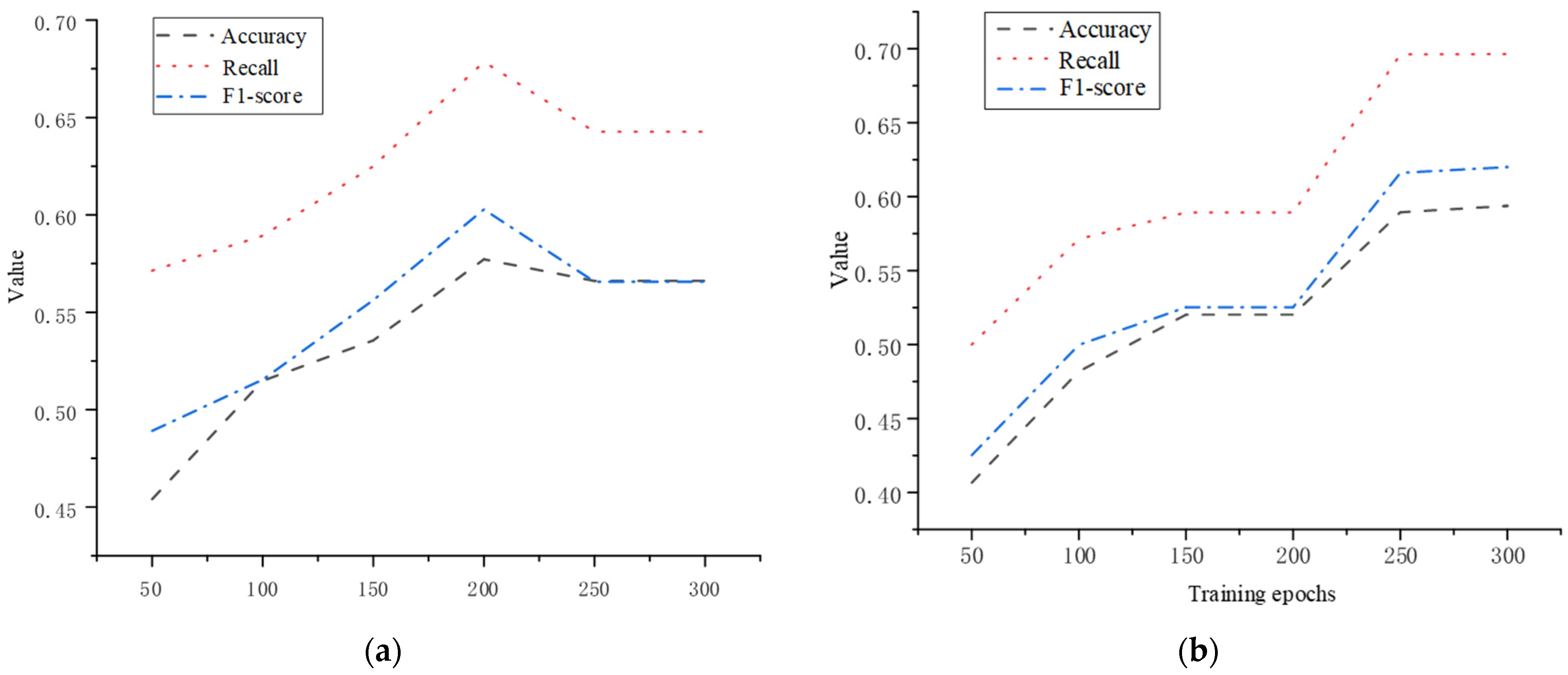
4.2. Model Verification Based on 1DCNN-BiLSTM-AdaBoost

The various performance metrics of the model are shown in Figure 8. By analyzing Figure 8, Figure 9 and Figure 10, we observe that the performance of the second and fifth weak classifiers declines significantly during the AdaBoost iteration process. This phenomenon primarily stems from the core mechanism of the AdaBoost algorithm: in each iteration, the sample weights are updated based on the classification errors of the previous weak classifier, ensuring that subsequent iterations focus more on samples that are prone to misclassification. While this dynamic weight adjustment mechanism may cause temporary performance drops in certain weak classifiers, it ultimately helps the ensemble model reduce the overall error rate, thereby enhancing final prediction accuracy and robustness. This behavior is a natural characteristic of AdaBoost’s weight adjustment process and reflects the model’s increased focus on difficult samples.

To better illustrate this process, Figure 9 presents the variation in the weights (Alpha values) of each weak classifier. The figure clearly shows how the weights change across different iterations. By observing the gradual increase in Alpha values, we can intuitively see that weak classifiers with higher overall weights play a more crucial role in the final decision-making process. This confirms that AdaBoost effectively emphasizes hard-to-classify samples, ultimately improving the model’s robustness.

Additionally, since the fault dataset used in this study is relatively balanced across different fault states, the accuracy and recall values remain close. To avoid redundancy in data visualization, we do not separately plot the accuracy curve. By evaluating cross-entropy loss, confusion matrices, and multiple performance metrics, we can comprehensively assess the model’s effectiveness. Overall, the introduction of the AdaBoost algorithm significantly enhances the model’s ability to capture complex data features, improving its accuracy and robustness in wind turbine blade fault detection tasks.

4.3. Algorithm Comparison and Verification

To validate the superiority of the 1DCNN-BiLSTM-AdaBoost model, we conducted performance experiments comparing it with the five other models listed in

Table 5. Model performance comparison.

Model	Metric 1	Metric 2	Metric 3	Metric 4
LSTM	0.6427	0.5661	0.6429	0.5673
BiLSTM	0.6964	0.5938	0.6967	0.6130
1D CNN	0.7400	0.6250	0.7400	0.6667
1D CNN-BiLSTM (Single-Channel)	0.7800	0.6450	0.7791	0.6863
1D CNN-BiLSTM (Dual-Channel)	0.9375	0.9500	0.9377	0.9395
Proposed Method (This Paper)	0.9688	0.9722	0.9692	0.9686

. The results, presented in Figure 8 and Table 5, highlight the performance differences across multiple evaluation metrics, such as accuracy, recall, and F1-score. These comparisons clearly demonstrate that the proposed 1DCNN-BiLSTM-AdaBoost model significantly outperforms the other models in various aspects. First, among the single-model comparisons, the 1DCNN model achieved the best performance within its category, with consistently high values across all evaluation metrics, indicating its effectiveness in processing time-series data. Second, the BiLSTM model improved accuracy by 5.37% compared to the traditional LSTM model, demonstrating that the bidirectional LSTM structure is more effective in capturing long- and short-term dependencies in time-series data. Furthermore, when using a single data source, the 1DCNN-BiLSTM model improved accuracy by 6.10% over the standalone 1DCNN model, proving that the information fusion strategy effectively enhances diagnostic capabilities by integrating sensor data from different modalities. When incorporating dual-channel data fusion, the performance of the 1DCNN-BiLSTM model improved even further, highlighting the advantage of leveraging multiple data sources. Finally, after integrating the AdaBoost algorithm with the 1DCNN-BiLSTM model, all evaluation metrics improved by approximately 2–3%, confirming the effectiveness of ensemble learning in optimizing performance. The AdaBoost-enhanced model prioritizes misclassified samples, focusing on the model’s weaknesses during training, thereby improving overall accuracy and robustness.

In summary, the proposed 1DCNN-BiLSTM-AdaBoost model demonstrates clear advantages across all evaluation metrics, proving its high accuracy and robustness in wind turbine-blade fault detection. The key findings of this study can be summarized as follows: (1) BiLSTM outperforms traditional LSTM in capturing temporal dependencies; (2) 1DCNN effectively extracts local features; (3) Combining 1DCNN with BiLSTM enables the model to capture both local and global information, further enhancing prediction accuracy; (4) Multi-channel data fusion significantly improves overall model performance; (5) The integration of the AdaBoost ensemble strategy enhances weak classifiers, allowing the final model to achieve optimal performance in wind turbine blade fault detection tasks.

5. Conclusions

In view of the low accuracy of blade fault identification, it is proposed to use multi-source data to identify faults and broaden the source of fault information. At the same time, the 1DCNN-BiLSTM-AdaBoost algorithm model is innovatively proposed for fault type classification. Through the comparison of model performance, it is found that the 1DCNN-BiLSTM algorithm has a better effect than the use of 1DCNN, BiLSTM, and other models alone. And after multi-channel data fusion, the performance of the 1DCNN-BiLSTM model is further improved. At the same time, through experimental verification, the AdaBoost algorithm has a good optimization effect on weak classifiers. After multiple runs, the improvement effect on the model is about 2~10%. The model proposed in this paper uses a large amount of data, which can meet the actual needs of wind turbine blade fault diagnosis. Although the proposed 1D CNN-BiLSTM-AdaBoost model achieved satisfactory performance on the ZENODO dataset, several challenges remain when deploying it in real-world wind turbine systems. These include data diversity, sensor configuration differences, real-time processing requirements, and system integration complexities. Future work will focus on expanding data sources, exploring domain adaptation techniques, and developing online update mechanisms to enhance the model’s robustness and generalization capability. These efforts aim to provide more reliable technical support for intelligent maintenance and fault diagnosis in practical applications.

In the future, this research is expected to have a profound impact on intelligent monitoring and maintenance of wind energy and other renewable energy systems, facilitating a transition toward data-driven and intelligent operations. Further studies could focus on enhancing the system’s adaptability to varying operating conditions and integrating emerging technologies such as IoT and big data analytics. These efforts aim to develop a more comprehensive, real-time, and efficient fault diagnosis framework, providing robust support for the safe and stable operation of renewable energy generation.

References

1. Zhao, D.; Shao, D.; Cui, L. CTNet: A data-driven time-frequency technique for wind turbines fault diagnosis under time-varying speeds. ISA Trans. 2024, 154, 335–351. [Google Scholar]
2. Jian, T.; Cao, J.; Liu, W.; Xu, G.; Zhong, J. A novel wind turbine fault diagnosis method based on compressive sensing and lightweight squeezenet model. Expert Syst. Appl. 2025, 260, 125440. [Google Scholar]
3. Shi, P.; Jia, L.; Yi, S.; Han, D. Wind turbines fault diagnosis method under variable working conditions based on AMVMD and deep discrimination transfer learning network. Meas. Sci. Technol. 2024, 35, 046120. [Google Scholar]
4. Zhao, K.; Liu, Z.; Li, J.; Zhao, B.; Jia, Z.; Shao, H. Self-paced decentralized federated transfer framework for rotating machinery fault diagnosis with multiple domains. Mech. Syst. Signal Process. 2024, 211, 111258. [Google Scholar]
5. Ren, X.; Wang, S.; Zhao, W.; Kong, X.; Fan, M.; Shao, H.; Zhao, K. Universal federated domain adaptation for gearbox fault diagnosis: A robust framework for credible pseudo-label generation. Adv. Eng. Inform. 2025, 65, 103233. [Google Scholar]
6. Liu, Y.; Jiang, H.; Yao, R.; Zeng, T. Counterfactual-augmented few-shot contrastive learning for machinery intelligent fault diagnosis with limited samples. Mech. Syst. Signal Process. 2024, 216, 111507. [Google Scholar]
7. Chao, Q.; Gao, H.; Tao, J.; Liu, C.; Wang, Y.; Zhou, J. Fault diagnosis of axial piston pumps with multi-sensor data and convolutional neural network. Front. Mech. Eng. 2022, 17, 36. [Google Scholar] [CrossRef]
8. Guo, Y.; Mao, J.; Zhao, M. Rolling bearing fault diagnosis method based on attention CNN and BiLSTM network. Neural Process. Lett. 2023, 55, 3377–3410. [Google Scholar]
9. Fu, G.; Wei, Q.; Yang, Y.; Li, C. Bearing fault diagnosis based on CNN-BiLSTM and residual module. Meas. Sci. Technol. 2023, 34, 125050. [Google Scholar]
10. Hong, D.; Kim, B. 1D convolutional neural network-based adaptive algorithm structure with system fault diagnosis and signal feature extraction for noise and vibration enhancement in mechanical systems. Mech. Syst. Signal Process. 2023, 197, 110395. [Google Scholar]
11. Wang, Q.; Cao, D.; Zhang, S.; Zhou, Y.; Yao, L. The Cable Fault Diagnosis for XLPE Cable Based on 1DCNNs-BiLSTM Network. J. Control Sci. Eng. 2023, 2023, 1068078. [Google Scholar]
12. Wang, X.; Mao, D.; Li, X. Bearing fault diagnosis based on vibro-acoustic data fusion and 1D-CNN network. Measurement 2021, 173, 108518. [Google Scholar]
13. Eren, L.; Ince, T.; Kiranyaz, S. A generic intelligent bearing fault diagnosis system using compact adaptive 1D CNN classifier. J. Signal Process. Syst. 2019, 91, 179–189. [Google Scholar]
14. Chen, C.C.; Liu, Z.; Yang, G.; Wu, C.C.; Ye, Q. An improved fault diagnosis using 1d-convolutional neural network model. Electronics 2020, 10, 59. [Google Scholar] [CrossRef]
15. Huang, T.; Zhang, Q.; Tang, X.; Zhao, S.; Lu, X. A novel fault diagnosis method based on CNN and LSTM and its application in fault diagnosis for complex systems. Artif. Intell. Rev. 2022, 55, 1289–1315. [Google Scholar]
16. Shi, J.; Peng, D.; Peng, Z.; Zhang, Z.; Goebel, K.; Wu, D. Planetary gearbox fault diagnosis using bidirectional-convolutional LSTM networks. Mech. Syst. Signal Process. 2022, 162, 107996. [Google Scholar]
17. Zhao, K.; Jia, F.; Shao, H. Unbalanced fault diagnosis of rolling bearings using transfer adaptive boosting with squeeze-and-excitation attention convolutional neural network. Meas. Sci. Technol. 2023, 34, 044006. [Google Scholar]
18. Guo, J.; Song, X.; Liu, C.; Zhang, Y.; Guo, S.; Wu, J.; Cai, C.; Li, Q. Research on the Icing Diagnosis of Wind Turbine Blades Based on FS-XGBoost-EWMA. Energy Eng. 2024, 121, 1739–1758. [Google Scholar]
19. An, G.; Jiang, Z.; Cao, X.; Liang, Y.; Zhao, Y.; Li, Z.; Dong, W.; Sun, H. Short-term wind power prediction based on particle swarm optimization-extreme learning machine model combined with AdaBoost algorithm. IEEE Access 2021, 9, 94040–94052. [Google Scholar]
20. Singh, S.K.; Khawale, R.P.; Hazarika, S.; Bhatt, A.; Gainey, B.; Lawler, B.; Rai, R. Hybrid physics-infused 1D-CNN based deep learning framework for diesel engine fault diagnostics. Neural Comput. Appl. 2024, 36, 17511–17539. [Google Scholar]
21. He, D.; Lao, Z.; Jin, Z.; He, C.; Shan, S.; Miao, J. Train bearing fault diagnosis based on multi-sensor data fusion and dual-scale residual network. Nonlinear Dyn. 2023, 111, 14901–14924. [Google Scholar]
22. Zhang, Z.; Jiao, Z.; Li, Y.; Shao, M.; Dai, X. Intelligent fault diagnosis of bearings driven by double-level data fusion based on multichannel sample fusion and feature fusion under time-varying speed conditions. Reliab. Eng. Syst. Saf. 2024, 251, 110362. [Google Scholar]
23. Wang, D.; Li, Y.; Song, Y.; Zhuang, Y. Bearing Fault Diagnosis Method based on Multiple-level Feature Tensor Fusion. IEEE Sens. J. 2024, 24, 23108–23116. [Google Scholar] [CrossRef]
24. Xu, X.; Song, D.; Wang, Z.; Zheng, Z. A Novel Collaborative Bearing Fault Diagnosis Method Based on Multisignal Decision-level Dynamically Enhanced Fusion. IEEE Sens. J. 2024, 24, 34766–34776. [Google Scholar] [CrossRef]
Figure 1. Structure of the 1D CNN-BiLSTM-AdaBoost model.
Applsci 15 03440 g001
Figure 2. Basic principle of the 1D CNN.
Applsci 15 03440 g002
Figure 3. Basic principle of LSTM.
Applsci 15 03440 g003
Figure 4. Basic principle of BiLSTM.
Applsci 15 03440 g004
Figure 5. Principle of AdaBoost.
Applsci 15 03440 g005
Figure 6. Training process.
Applsci 15 03440 g006
Figure 7. (a) Loss function for 128 neurons; (b) loss function for 256 neurons; (c) loss function for 32 neurons; (d) loss function for 64 neurons.
Applsci 15 03440 g007
Figure 8. Indicators in model operation.
Applsci 15 03440 g008
Figure 9. Weights of each weak classifier.
Applsci 15 03440 g009
Figure 10. (a) LSTM index graph; (b) BiLSTM index graph; (c) 1DCNN index graph; (d) 1DCNN-BiLSTM (single-channel data) index graph.
Applsci 15 03440 g010aApplsci 15 03440 g010b