1. Introduction
The concept of Simultaneous Localization and Mapping (SLAM) [
1] emerged as a fundamental problem in mobile robotics, initially addressed by probabilistic methods such as EKF-SLAM [
2], FastSLAM [
3], and Graph-SLAM [
4], which used Kalman filters and graphs for trajectory and map estimation. In the last decade (2015 to 2025), the number of publications related to SLAM per year has increased by 292.7% [
5], reflecting growing interest and advancements in the field. With advances in computing, visual approaches such as ORB-SLAM [
6], LSD-SLAM [
7], and DSO [
8] improved real-time pose estimation. In the context of autonomous driving, sensor fusion has become essential for handling dynamic environments, leading to the development of methods such as LIO-SAM [
9] and VINS-Mono [
10], which integrate LiDAR and IMU data to enhance localization accuracy.
Recently, the state of the art in SLAM has incorporated deep-learning-based techniques, such as DeepVO [
11] and CodeSLAM [
12], which leverage neural networks to learn compact environment representations and improve the robustness of visual odometry. Additionally, innovative approaches like NeRF-SLAM [
13], 3D Gaussian Splatting [
14], and NICE-SLAM [
15] explore implicit representations to enhance high-fidelity 3D scene reconstruction. Hybrid methods such as R3LIVE [
16] and NeRF-LOAM [
17] combine the advantages of classical and modern techniques to overcome challenges in unstructured environments and variable lighting conditions. The integration of SLAM with Large Language Models (LLMs) [
18] and semantic perception systems, such as SuMa++ [
19] and SemanticKITTI [
20], has demonstrated advancements in understanding complex scenes.
In the current landscape, approaches like DL-SLOT [
21] and LIO-SEGMOT [
22] incorporate multi-object tracking to handle dynamic obstacles, while ClusterSLAM [
23] and TwistSLAM [
24] improve odometry accuracy in dense urban scenarios. These advancements show SLAM evolving to meet autonomous vehicle demands.
Despite these advancements, one of the key challenges in SLAM remains ensuring the completeness of the generated maps. SLAM allows robots to map and localize simultaneously. This capability is crucial for applications ranging from autonomous vehicles [
25] to space exploration [
26]. Ensuring full coverage, especially in dynamic scenarios, remains a challenge.
Traditional SLAM approaches often rely on random or exploratory navigation methods that, although capable of covering most of the environment, lack efficient mechanisms to systematically explore unmapped regions [
1]. This leads to shadowed areas, redundant paths, and map gaps [
27,
28]. Industrial robots need efficient mapping for logistics and safety. In search-and-rescue, full coverage is vital for finding survivors. The ability to accurately detect and close unexplored areas makes MARS-SLAM particularly suitable for these domains, where incomplete maps could lead to inefficiencies or critical mission failures.
Moreover, conventional methods lack a deterministic process to verify mapping completion, often resulting in unnecessary exploration that wastes time, energy, and computational resources. To address these challenges, this research proposes MARS-SLAM, a novel approach that enhances mapping completeness through the use of virtual markers placed in unexplored regions. These markers, derived from LiDAR sensor readings, dynamically guide the robot’s exploration, ensuring systematic coverage while optimizing resource usage. The key contributions of this study are:
- 1.
A marker-based methodology for identifying and tracking unexplored areas, enabling a structured exploration process that minimizes redundant revisits.
- 2.
An adaptive navigation strategy that prioritizes markers based on their distance and antiquity, improving mapping efficiency.
- 3.
An optimized path-finding system that enhances navigation efficiency when direct access to a target marker is obstructed.
- 4.
A method for identifying mapping completion, ensuring that the exploration process effectively detects when the environment has been fully mapped.
To visually illustrate the structure of MARS-SLAM and its contributions,
Figure 1 presents a mind map summarizing the main components of our methodology. This diagram provides an intuitive overview of the proposed approach, highlighting its core mechanisms and objectives. Despite its advantages, MARS-SLAM faces challenges in highly dynamic environments, where frequent and unpredictable obstacles can interfere with the correct inclusion of markers. In highly dynamic environments, the main difficulty lies in the ever-changing nature of the scenario, which can compromise the reliability of the marking system and, consequently, the accuracy of navigation. Since MARS-SLAM relies on the placement and tracking of virtual markers to guide exploration, any unexpected change in the environment can render previously registered markers obsolete. For example, if a marker is placed in an area that later becomes inaccessible due to the emergence of a moving obstacle, the robot may fail in its attempt to reach that region, requiring constant reassessments of the exploration strategy.
Thus, the research presented in this paper aims to answer the following question: How can the use of markers to identify unexplored regions optimize the SLAM process, ensuring completeness and accuracy of mapping in unknown environments?
Section 2 reviews related works, exploring existing SLAM approaches and identifying the gaps that our methodology seeks to address. In
Section 3, a detailed description of MARS-SLAM is provided, including the flowchart and strategies implemented for the method’s operation.
Section 4 presents the experimental results obtained in various scenarios. Finally,
Section 5 concludes the paper, discussing the contributions and limitations of MARS-SLAM, as well as suggesting potential directions for future research.
3. Marker-Assisted Region Scanning
To ensure the effective and accurate completion of mapping, a method is proposed that utilizes markers to identify and track unexplored regions on the map. The primary goal of this method is to ensure that all areas of the environment are mapped, avoiding gaps that could compromise the navigability and usefulness of the generated map. The markers play a role in this process, serving as indicators of regions that still need to be explored. As the robot progresses in building the map, it adds markers to unexplored areas based on sensor readings. These markers are stored in a list, which, over time, reflects the mapping progress. The mapping process is considered complete when the marker list is empty, indicating that no unexplored regions remain.
Initially, the robot performs a full 360° rotation, analyzing the surrounding environment and placing markers in unexplored areas, with the goal of ensuring complete coverage of the spaces around the robot. Once the full rotation is complete, the robot selects one marker as the target and moves toward that marker. The robot then chooses the next most suitable marker and repeats the process. This cycle of marker selection and navigation continues until all markers have been removed, indicating that the mapping of the environment is complete. The detailed steps of the method are described in Algorithm 1.
3.1. Update Robot State
This process continuously updates the robot’s state during navigation, determining its new pose and LiDAR measurements based on the current action and the specified target. It plays a role in maintaining the robot’s alignment with its goal, dynamically adjusting its trajectory as needed and gathering essential data to support the ongoing mapping of the environment. The algorithm plays a vital role in enabling the robot to adapt its trajectory as needed, allowing for real-time decision making that enhances its ability to navigate complex spaces.
Algorithm A1 requires the robot’s current pose (
), target marker (
), executed action (
A), grid map (
G), and path list (
). It outputs the updated pose (
) and LiDAR measurements (
L). The process involves three main steps: identifying the assigned action (rotation or movement), updating the pose and LiDAR readings, and checking for obstacles. If the path is clear, the robot moves directly to the marker. Otherwise, a path-planning algorithm determines an alternative route, storing intermediate points in
to navigate around obstacles.
| Algorithm 1 Marker-Assisted Region Scanning |
Ensure: Grid map of the environment (G)
- 1:
G {Grid map with all cells as unknown (gray pixels)} - 2:
{Pose list, marker list, LiDAR measurements and path} - 3:
{Target marker} - 4:
k - 5:
← initial position - 6:
while full rotation not completed do - 7:
{Algorithm A1} - 8:
- 9:
{Algorithm A2} - 10:
k←k + 1 - 11:
end while - 12:
while do - 13:
if is null then - 14:
{Algorithm A3} - 15:
end if - 16:
- 17:
- 18:
if has been reached then - 19:
; - 20:
end if - 21:
{Algorithm A4} - 22:
- 23:
k←k + 1 - 24:
end while
|
3.2. Marker Addition
Markers are created based on readings from the LiDAR, a sensor used by the robot to scan the environment. Each measurement provides the distance to the first obstacle detected along that direction. The LiDAR has a maximum range, beyond which the measurements are not considered. During the robot’s movement, at each registered pose, all LiDAR measurements are analyzed to identify potential obstacle-free areas. To ensure that markers are efficiently distributed without redundancy, the algorithm imposes a restriction: a new marker can only be added if no other marker exists within a predetermined minimum distance. This criterion is enforced by calculating the Euclidean distance between the new marker and all previously placed markers, ensuring proper spacing and preventing unnecessary overlap.
Figure 2 illustrates the process of identifying free areas and adding markers.
Algorithm A2 takes the grid map (
G), LiDAR measurements (
L), and the existing marker list (
M) as input. It checks whether a new marker can be placed by verifying if the corresponding area is still unknown (represented by a gray pixel) and if it satisfies the minimum distance requirement
. If both conditions are met, a new marker is added. If a marker already exists nearby, the algorithm examines neighboring cells for unexplored areas before placing a new marker.
Figure 2 illustrates this process.
3.3. Marker Selection
After the initial navigation period, the robot needs to choose a marker as a target to map an unexplored area. For this selection, the robot identifies markers that have free access, meaning it is possible to plot a direct path from the robot’s current position to the marker without encountering obstacles. Once the markers with free access are identified, the robot uses two criteria to select the target marker: age and distance. Each marker is associated with a specific pose, recorded in a pose list starting from pose 0 up to the robot’s current pose. For example, a marker created at pose 10 is considered older than one create at pose 50. The robot then selects between the oldest marker and the closest marker. If the distance to the oldest marker is more than times the distance to the closest marker, the closest marker is chosen as the target ( is a parameter adjusted based on the desired navigation behavior). Otherwise, the oldest marker is selected. When there are no markers with free access, the robot selects a target marker using the tournament method.
Algorithm A3 describes this logic in a structured way, starting with the filtering of markers with free access () and, if no such markers are found, applying the tournament selection method. After filtering the accessible markers, the algorithm then considers the distance () and the age of the oldest marker (), and compares it with the distance to the closest marker (). Based on this comparison and the parameter , the algorithm determines the target marker () that will guide the robot in its next exploration step. This efficient selection process allows the robot to balance the exploration of new areas with older markers while also considering the need to optimize the path by prioritizing closer markers when appropriate.
3.4. Marker Removal
Marker removal is a step to ensure that the map remains up to date, reflecting only the areas that still need to be explored. During the robot’s navigation, at each step, it is checked whether any of the previously added markers are located in a region that has already been mapped. Specifically, a marker is removed when its cell, as well as the neighboring cells, are no longer unknown.
Figure 3 illustrates the process of map updating and the subsequent removal of markers during the robot’s navigation.
Figure 3a shows the map being updated as the robot maps new areas. In these updates, previously unknown regions are converted into mapped areas, indicating that the robot has already explored these cells.
Figure 3b demonstrates the marker removal process.
Algorithm A4 takes the grid map (
G) and marker list (
M) as input and returns an updated list (
) containing only markers in unexplored regions. The process iterates through each marker’s coordinates
and checks if the corresponding cell in
G is still unknown. If the area has been fully mapped, the marker is discarded. If any neighboring cell remains unexplored, the marker is retained. This ensures that only markers in unknown regions are preserved, improving mapping efficiency.
Figure 3 illustrates this process.
3.5. Path Finding
In the situation where the target marker does not have free access, the robot needs to return to the pose where the target marker is created to ensure a clear path to the target. To optimize the path, a method is developed to reduce the set of poses needed to reach the target marker. The approach leverages the known path recorded in the pose list to determine the smallest set of poses that connect the robot’s current position to the target marker. The method operates as follows: starting from the robot’s current position, poses are traversed at intervals defined by a previously established constant until the target marker’s pose is reached. At each step, the closest pose in the pose list index to the target marker’s pose that has a free path to the current position is identified.
The specifics of this procedure are detailed in Algorithm A5. Initially, the algorithm sets the path
as an empty list and defines a search step size
s. A loop continues until a valid path is found. In each iteration, the algorithm generates a set of candidate poses
by calculating the indices based on the target marker’s pose index
and the current pose index
k, considering increments defined by the search step size. If there are no candidate poses available, the loop terminates. For each pose in the candidate set
, the algorithm checks for obstacles between the current pose and the candidate pose. If a clear path is identified (i.e., no obstacles), the algorithm updates the path
by adding the candidate pose and then updates the current pose index
k to the candidate pose. This process repeats until a direct, obstacle-free route is established between the robot’s current position and the target marker.
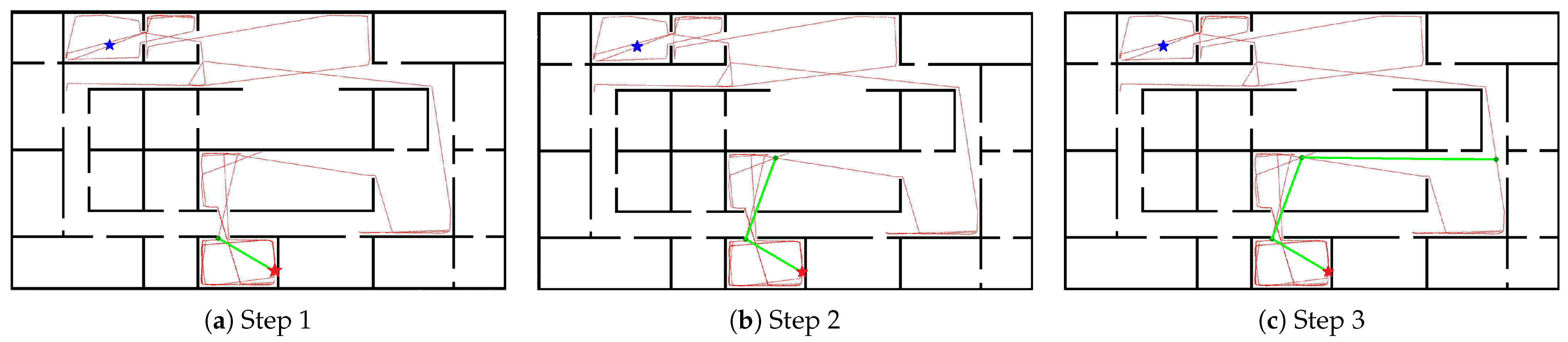
Figure 4 visually illustrates this path optimization process, demonstrating the stages of checking and selecting intermediate poses until the final path is defined.
4. Simulation Platform
The MARS-SLAM simulation platform models autonomous robot navigation in complex virtual environments. The system employs a robot with a LiDAR sensor to map surroundings, detect obstacles, and explore uncharted regions using marker-based search. Developed in Python, it uses Pygame for visualization and Pandas for data management. The platform simulates a 2D environment where the robot scans and updates an occupancy map in real time.
Algorithm 2 describes the simulation’s execution flow, divided into six stages. The algorithm starts with initializing the simulation environment and instantiating the robot, with its properties specific to each map, including LiDAR range, obstacle avoidance distance, motor speed parameters, and a conversion factor for meters to pixels. During the simulation, the robot captures user events, clears the screen, updates its position, detects obstacles, updates movement control, and maps the environment. In each iteration, the robot is graphically rendered on the screen, and the map display is updated, providing a visual representation of the navigation progress.
| Algorithm 2 MARS-SLAM Simulation |
- 1:
- 2:
- 3:
while simulation running do - 4:
capture user events - 5:
clear the screen - 6:
- 7:
- 8:
- 9:
- 10:
render robot on the screen - 11:
update map display - 12:
end while - 13:
end simulation
|
4.1. Simulation Environment Initialization
The virtual environment used in MARS-SLAM simulations is generated from a grayscale PNG image, with dimensions of 900 by 1600 pixels. Each pixel of the image corresponds to a unique coordinate in the simulated environment, representing a position on the map that the robot will explore. The image is loaded and processed by the simulator, which interprets the different grayscale values to define the navigability of the environment. White pixels (255, 255, 255) indicate free areas, where the robot can move without restrictions, while black pixels (0, 0, 0) represent obstacles on the map, marking regions where the robot cannot enter. Among the various mapping techniques, metric maps stand out for their detailed and precise nature [
36]. Metric maps provide a detailed representation of the environment’s geometry, describing the shape, dimensions, and arrangement of objects.
Metric maps are essential in robotics for describing the environment’s geometry with high accuracy. Mathematically, a metric map is modeled as a matrix where each cell, or pixel, represents a specific state of the environment. This text describes how a metric map works, focusing on the mathematical representation and the states of the pixels. A metric map is represented as a matrix M of size , where each element represents a cell in the environment. The cell can be in one of three states:
Free (White | 255, 255, 255): The cell is free of obstacles.
Occupied (Black | 0, 0, 0): The cell contains an obstacle.
Unknown (Gray | 150, 150, 150): The state of the cell has not been determined.
By using this image as a base, the simulator transforms the graphical representation into a coordinate grid, where each pixel is associated with a cell in the occupancy map. This approach allows the robot to accurately locate its position in the environment and update the map according to the explored or avoided areas. The simulation platform allows real-time graphical rendering of the environment and the robot. The map image is loaded into memory, and its visualization is configured so that the regions explored by the robot during the simulation are overlaid on the base map. Thus, the exploration progress is displayed in real time, with the path traveled and the mapped areas highlighted.
4.2. Robot Instantiation
The robot is modeled based on a simple kinematic system, where the left and right motor speeds control its direction and linear velocity. The initial speed of both motors is set as , while the maximum configured speed is . The robot’s initial position is randomly selected within the map’s boundaries. The robot is positioned with coordinates in meters, converted to pixels using a conversion rate. The initial orientation () is also randomly defined, covering the range from to .
The LiDAR sensor is simulated to take measurements in
nM directions, covering a field of view of angle
degrees with a configurable maximum of
pixel. It is used to detect obstacles within this field of view and maximum distance. The robot is programmed to avoid obstacles that are within a distance of
pixel. If an obstacle is detected within this limit, the robot adjusts its direction to avoid collisions by calculating the evasion angle based on the LiDAR readings. The evasion direction is stored in control variables, and the robot continues its path after the correction. The parameters used in the robot’s instantiation are detailed in
Table 3.
4.3. Robot Position Update
The robot’s position is updated based on the left (
) and right (
) motor speeds, which determine both linear and angular movement. These speeds are used to calculate the variation in the robot’s position and orientation in space. The robot’s linear velocity (
v) can be calculated as the average of the left (
) and right (
) motor velocities:
Additionally, the robot’s angular velocity (
w) can be determined from the motor velocities and the distance between the robot’s wheels (
L):
To calculate the variations in the robot’s
x and
y coordinates, as well as its orientation
, the differential motion equations can be used. Suppose that during a small time interval
, the robot moves with velocities
v and
w. The variations in the
x and
y coordinates and in the orientation
can be calculated as follows:
These equations describe the variations in the robot’s position and orientation based on the left and right motor velocities and the time interval . They are essential for predicting the change in the robot’s pose in a 2D mobile robotics environment.
4.4. Obstacle Detection
Obstacle detection is performed by the robot’s LiDAR sensor, which checks for the proximity of objects around the robot to avoid collisions. The process focuses on analyzing a limited subsection of the LiDAR’s field of view, corresponding to the range from −25 to +25 relative to the robot’s current orientation. This choice aims to reduce processing time and concentrate resources on detecting obstacles directly in front of the robot, which are more relevant for immediate navigation.
The LiDAR sensor takes distance measurements in various directions within this range, and the data from each measurement are compared to a predefined minimum distance threshold, called mOd. If an obstacle is detected at a distance less than or equal to this value, it is identified as a potential obstacle, and its information, such as the measured distance and detection angle, is stored in an obstacle list. This process is repeated for all measurements within the defined field of view, ensuring the robot has a clear and updated view of nearby obstacles. The detection is continuous, allowing the robot to adjust its path as necessary to avoid collisions. The obstacle position information is then used by the robot’s control system to efficiently avoid obstacles.
4.5. Movement Control Update
The robot’s movement control is based on the angular speeds of the wheels: (right wheel) and (left wheel). This control is adjusted according to obstacle detection and autonomous navigation using the MARS-SLAM method. The robot alternates between avoiding obstacles and navigating toward predefined markers, depending on environmental conditions.
Initially, the algorithm checks if the mapping process has been completed. If the mapping is complete, the robot stops its movement, setting and to zero. If the mapping is still ongoing, the robot continues navigating by adjusting its movement according to the marker position and obstacles in the environment. This control mechanism allows the robot to follow the exploration strategy and avoid obstacles simultaneously, ensuring that the robot navigates smoothly through the environment while maintaining safety and efficient exploration.
4.6. Environment Mapping
During navigation, the robot uses the LiDAR sensor to scan its surrounding environment. This mapping process involves continuous data capture, which are stored in a dataframe, serving as the main repository of simulation data. Each row in the dataframe records a state of the robot at a given time instance, including information such as position, orientation, and LiDAR readings. The structure of these data allows for a detailed analysis of the robot’s behavior over time and enables precise tracking of the environment’s exploration.
The LiDAR performs measurements within a 180-degree field of view, ranging from −90 to +90 relative to the robot’s current orientation. At each simulation step, a set of distance readings is generated, where each reading corresponds to the distance to the nearest obstacle along a specific direction. These readings, along with the robot’s coordinates (x, y) and its orientation (), are stored in the dataframe, which is updated at each simulation step. The captured data include:
Distance readings: The distances measured by the LiDAR to the detected obstacles along each scan angle.
Coordinates (x, y): The robot’s actual position in the environment.
Orientation (): The angle representing the robot’s direction.
Timestamp: A time record that allows synchronization and temporal analysis of the data.
The data collected by the LiDAR are used to build a grid map of the environment. This map is composed of pixels where white pixels represent free space and black pixels represent obstacles. For each LiDAR measurement, the distance to the nearest obstacle and the corresponding scan angle (relative to the robot’s orientation) are used to calculate the position of the obstacle. The position of the obstacle is determined using the following equations:
where
d is the distance measured by the LiDAR,
is the scan angle,
are the coordinates of the pose,
is the orientation of the pose. After calculating the position of the obstacle, a line of free space is drawn from the pose’s coordinates to the obstacle. This line draws each pixel along the path as free (white). This ensures that the robot has clear information about the explored areas without obstacles. Once the free space is marked, the position of the obstacle is updated in the grid map by marking a black point at the calculated obstacle position. This point represents the detected obstacle at that particular scan angle. This process is repeated for every LiDAR measurement at each pose. As the robot moves, the map is continuously updated to reflect the current state of the environment.
5. Results
In this section, the results of the experiments conducted to evaluate the efficiency and stability of the proposed MARS-SLAM method are presented. The experiments are obtained for three distinct scenarios, aiming to analyze the performance of the approach in various contexts. The maps of the virtual environments used in the simulations are shown in
Figure 5. The maps are designed with increasing levels of complexity, with Map 1 being the least complex, followed by the more challenging Map 2, and culminating in the highly complex Map 3, to thoroughly test the adaptability of the MARS-SLAM method. The simulations are performed on a computer with the following specifications: Intel(R) Core(TM) i7-10750H CPU @ 2.59 GHz, 24 GB of RAM, and Microsoft Windows 11 Home operating system (version 10.0.22631). The development environment and tools used for the implementation and simulations included Python 3.7.7 and the necessary libraries for calculations and visualization of the results.
5.1. Experiments
To provide a robust comparison of MARS-SLAM, two alternative routes are created. The objective of these simulations is to establish a solid basis for comparison with the new proposal. To achieve this, a pragmatic approach is developed that, under the assumption of prior knowledge of the map, allows for the distribution of markers in a grid format, with a distance proportional to the LiDAR scan limit. This distribution ensures that by visiting all the markers, the mapping is complete. These routes will provide an order of magnitude for evaluating the efficiency of MARS-SLAM. Comparing MARS-SLAM with these routes will help determine whether the method maps the whole map with a similar number of poses, even without prior knowledge of the environment. If MARS-SLAM yields comparable results to the alternative routes, this would indicate that the method is efficient, as it can achieve similar results even though it has no prior knowledge of the map. To compare MARS-SLAM, two alternative routes are developed using markers distributed in a grid:
- 1.
Standard Zigzag Route: In this route, the robot is positioned at the first marker of the first row and navigates from left to right in even rows and from right to left in odd rows, creating a zigzag pattern.
- 2.
ACO-Optimized Route: Here, a heuristic based on the Ant Colony Optimization (ACO) algorithm [
37] is applied to construct a route that is close to the optimal route.
These routes are generated for the three virtual scenarios shown in
Figure 5.
Figure 6 presents the final mapping results (100% completion) for all three maps, comparing the performance of the Zigzag, ACO, and MARS-SLAM methods. The already-mapped areas are shaded in pink, red dots represent the markers added by the robot, and the small pink dots indicate the robot’s recorded poses throughout the mapping process.
The simulations demonstrate that MARS-SLAM successfully achieves its main objective, which is to perform a complete mapping of the environment, utilizing an efficient stopping criterion to identify the conclusion of the navigation task. Each simulation is repeated 10 times to ensure the robustness of the results.
Table 4 presents the averages and standard deviations for the number of poses require for complete mapping by each method, as well as the mapping completeness.
Table 5 presents the average times and standard deviations related to three time categories: preprocessing, navigation, and total simulation time. The preprocessing time refers to the initial phase before navigation, which includes setting up specific parameters for each method. Navigation time, on the other hand, represents the period in which the robot is actively exploring the environment and mapping unknown regions. To assess the efficiency of the marker selection method, three distinct versions of MARS-SLAM are tested, each using a different marker selection method: Tournament (MST), Proximity (MSP), and Age (MSA). This approach aims to determine whether the selection method impacts the effectiveness of MARS-SLAM, allowing a comparative analysis of the results obtained with each selection strategy.
Figure 7 illustrates the comparison between the evaluated methods based on two criteria: the number of poses and the total simulation time.
Figure 7a compares the number of poses used by each method across the three maps;
Figure 7b compares the required simulation time. It is observed that for Maps 1 and 2, MARS-SLAM demonstrate consistency, showing a number of poses similar to the comparative methods. However, in Map 3, MARS-SLAM achieves significantly superior performance, using fewer poses, which validates its effectiveness in complex unknown environments.
Although simulation time is an important factor as it directly impacts resource costs during the SLAM process, it can be managed or even justified in many applications. On the other hand, the number of poses stands out as a more relevant indicator of the quality of the final mapping. A method that generates a complete map with a reduced number of poses demonstrates higher efficiency by avoiding redundancies and producing a more accurate and compact representation of the environment. As a result, the maps generated are more suitable for reuse and future applications since they contain sufficient data to efficiently represent the environment without compromising completeness. Thus, when evaluating the performance of MARS-SLAM, the number of poses becomes a criterion, reflecting the system’s ability to create optimized, high-quality maps while reducing unnecessary data overhead.
Table 6 presents the percentage variations in the number of poses when comparing different methods across three scenarios.
5.2. Discussion
Overall, MARS-SLAM yields superior results, particularly when combined with the MST strategy, which reduces the number of poses by 64.39% compare to ACO and 71.07% compare to Zigzag in Map 3. This significant reduction reflects the method’s efficiency in complex environments, such as Map 3, where the implementation of Zigzag and ACO requires the inclusion of a large number of markets. The increased number of markers made the optimization process too costly for ACO, which failed to find an efficient route within the simulation time limit. This reinforces the superiority of MARS-SLAM in handling complex environments, where its ability to reduce the number of poses translates into more efficient navigation and higher-quality mapping. A point to highlight is that MARS-SLAM is designed to operate in completely unknown environments, which significantly distinguishes it from the ACO and Zigzag methods. While these methods require prior knowledge of the map to distribute a marker grid that guides navigation, MARS-SLAM can autonomously explore and map unknown areas, adapting to real-time discoveries. This makes MARS-SLAM a more robust and versatile solution, as it does not depend on prior information or artificial setups to operate efficiently. Its ability to identify and explore unexplored regions adaptively, without the need for prior planning, positions it as a valuable tool for applications where the environment is entirely new or unpredictable.
In terms of completeness, as presented in
Table 4, all methods are able to fully map the environment, with minor variations in Map 3, where the complexity of the environment led to a slight reduction in mapping completeness for MST (99.8%) and MSP (99.5%). Among the 30 simulations conducted with MARS-SLAM on Map 3 (10 simulations for each strategy), in 2 of them, the method did not achieve 100% completeness. This occurs due to the specifics of the marker placement methodology, referred to as the shadow effect. As illustrated in
Figure 8, the shadow effect occurs due to a combination of factors related to the LiDAR’s functionality and the marker placement methodology in the system. This effect happens when the robot, while navigating through dense or narrow regions, fails to add markers correctly in all unmapped areas. As a result, the robot perceives some unexplored areas as already mapped, since the absence of markers indicates to it that the area has been explored. This issue is partly caused by the limited reading angle of the LiDAR, which only performs measurements from −90
to 90
, along with the strategy of adding new markers only at the limits of the LiDAR’s range when it detects no obstacles. In narrow environments, such as corridors or doorways, the robot may pass by a structure without successfully adding markers within the passage, as the LiDAR, depending on the robot’s orientation, may not capture the complete area (such as a narrow entrance). For example, when passing perpendicularly to a narrow doorway, the robot may only detect the doorframe and not “see” the inner space, which prevents markers from being placed in that area. This effect is also intensified in maps with dense structures, where marker dispersion is high and insufficient to cover all spaces, leading to a false perception of mapping completeness.
The shadow effect represents a critical challenge for complete mapping accuracy in MARS-SLAM, revealing the need for further investigation and improvements in the marker placement methodology. This phenomenon, which occurs mainly in narrow areas poorly detected by the LiDAR, indicates the need for adjustments in sensor configuration or complementary strategies to ensure these shadowed regions are properly mapped. Measures such as increasing marker density in more complex areas or adjusting LiDAR parameters could mitigate this effect and improve mapping completeness.
Moreover, despite the overall good performance of MARS-SLAM, particularly when compared to ACO and Zigzag, in more complex scenarios like Map 3, the challenges encountered in environments with many narrow zones or sharp angles highlight the difficulties in accurate marker placement. In these cases, the method may struggle with precise marker positioning, which in turn increases processing time and the complexity of navigation. Although MARS-SLAM still maintains a significant advantage over alternative approaches, these factors demonstrate the importance of enhancing the method to handle scenarios with low visibility or high obstacle density.
6. Conclusions
This paper proposed MARS-SLAM, a novel method that optimizes the Simultaneous Localization and Mapping process by leveraging markers to enhance navigation efficiency in unknown environments. Experimental results in three distinct virtual scenarios demonstrated that MARS-SLAM, particularly when combined with the MST strategy, significantly outperforms traditional approaches such as Zigzag and ACO. Notably, in the most complex scenario (Map 3), MARS-SLAM reduced the number of poses by 71.07% compared to Zigzag and 64.39% compared to ACO, highlighting its efficiency in minimizing redundant movements while maintaining mapping accuracy.
MARS-SLAM’s capability to autonomously explore unknown environments without requiring prior map knowledge makes it a robust and adaptable solution. Unlike Zigzag and ACO, which rely on predefined marker grids, MARS-SLAM dynamically identifies unexplored regions, ensuring efficient coverage with fewer poses. However, challenges remain in highly constrained environments, where the shadow effect from marker placement can impact mapping completeness. Future work should focus on refining sensor configurations, optimizing marker distribution, and adapting the method to dynamic environments with moving obstacles.
Additionally, real-world validation is essential to confirm the method’s applicability. Although our current implementation was developed and validated in a simulated environment, careful consideration was given to its feasibility in real-world applications. The method is already structured to handle data storage and manipulation in a manner compatible with microcontrollers, and the same control commands used in simulation can be applied to a real robotic system. However, real-time SLAM must be incorporated to ensure continuous localization during mapping. Furthermore, porting the MARS-SLAM code from Python to C++ is necessary to meet the computational constraints of embedded systems.
Another important research direction is the evaluation of alternative sensor configurations beyond LiDAR. While LiDAR provides high-precision mapping, incorporating additional sensors can improve the system’s ability. Adapting MARS-SLAM to work with RGB-D cameras, stereo vision, or radar requires refining the unmapped region detection algorithm to ensure accurate marker placement.


