
Seismic Performance of Modal Transfer Stations on Soft Clays


Abstract
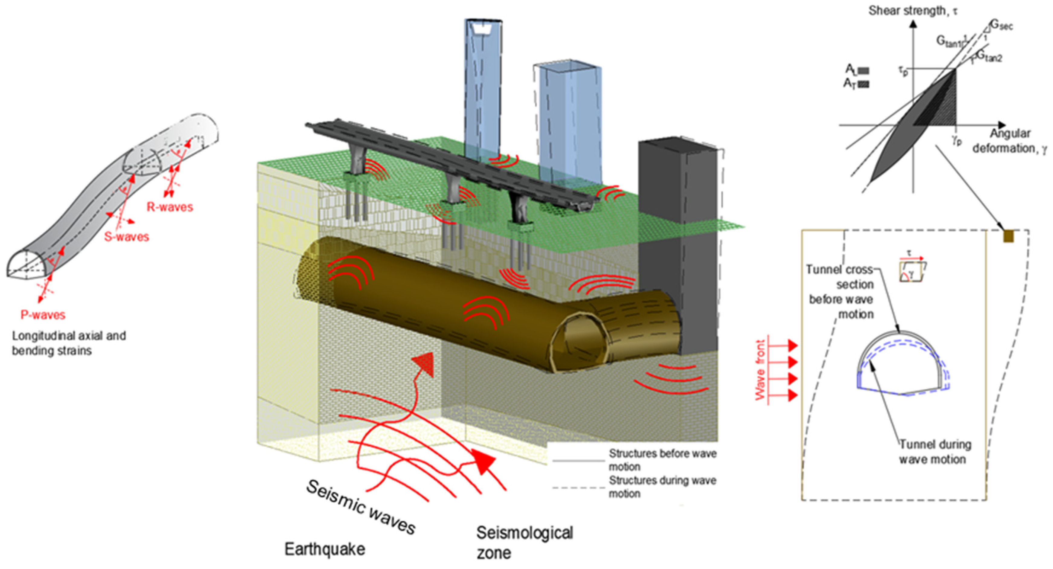
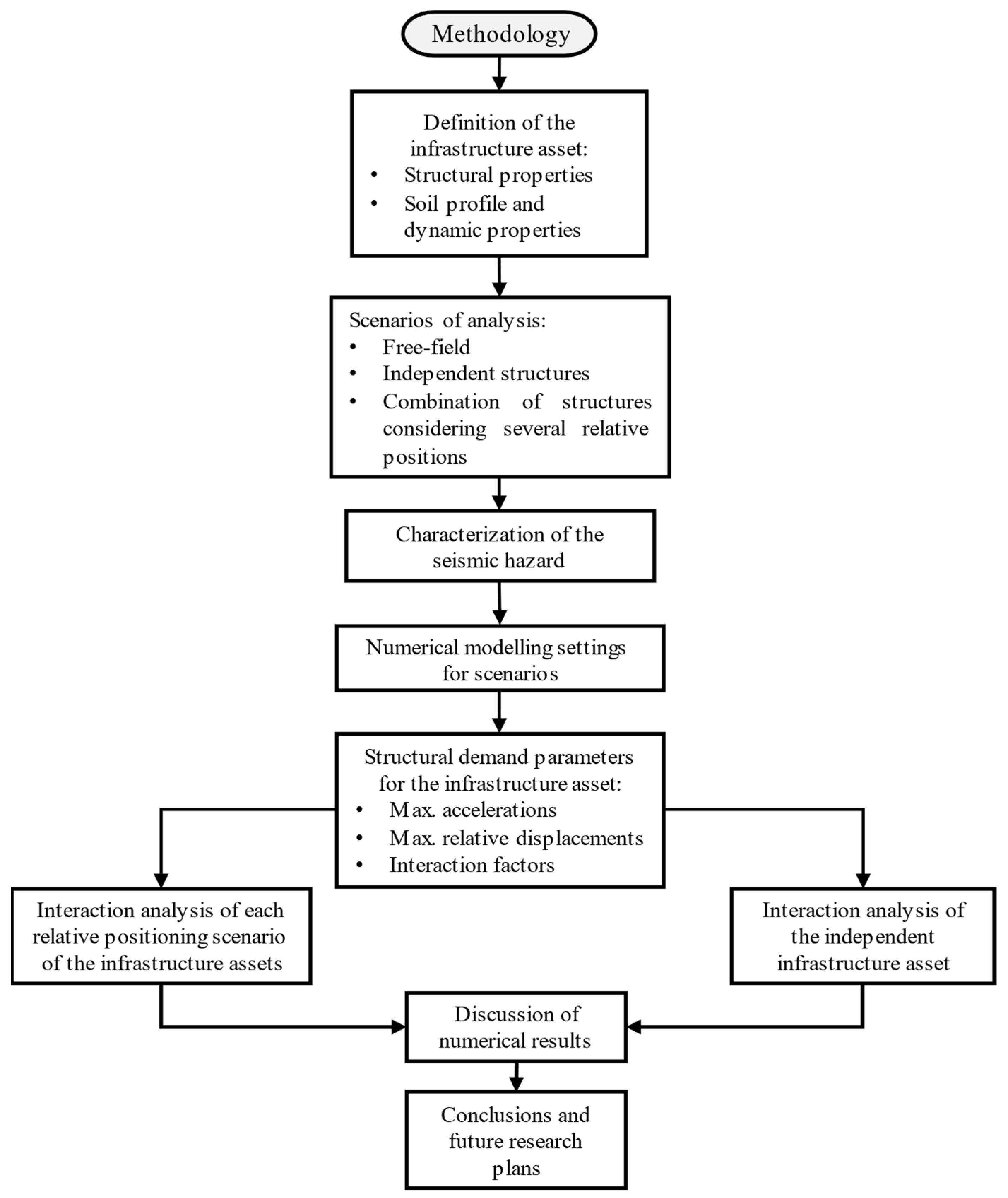
1. Introduction
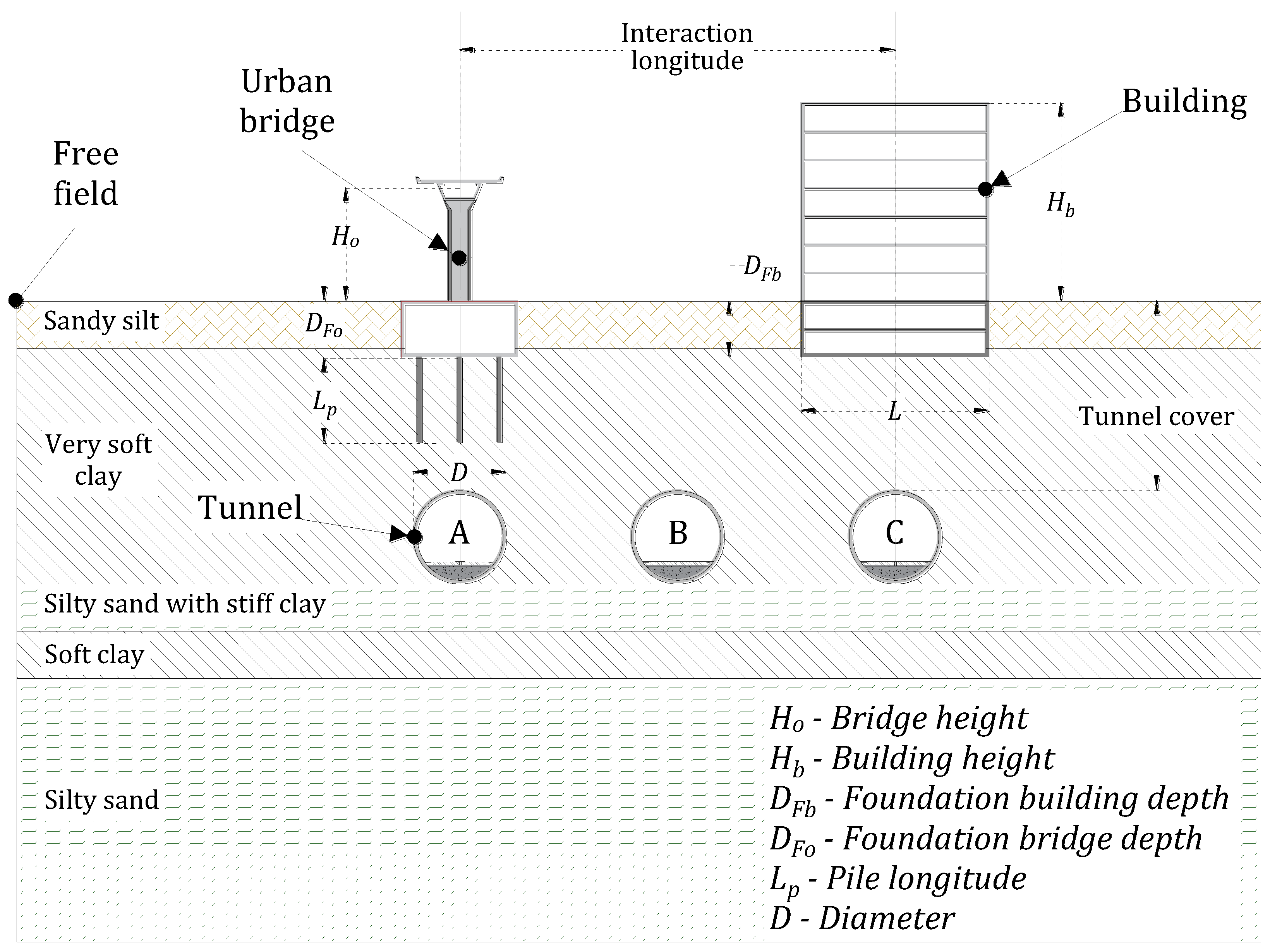
2. Definition of the Infrastructure Assets
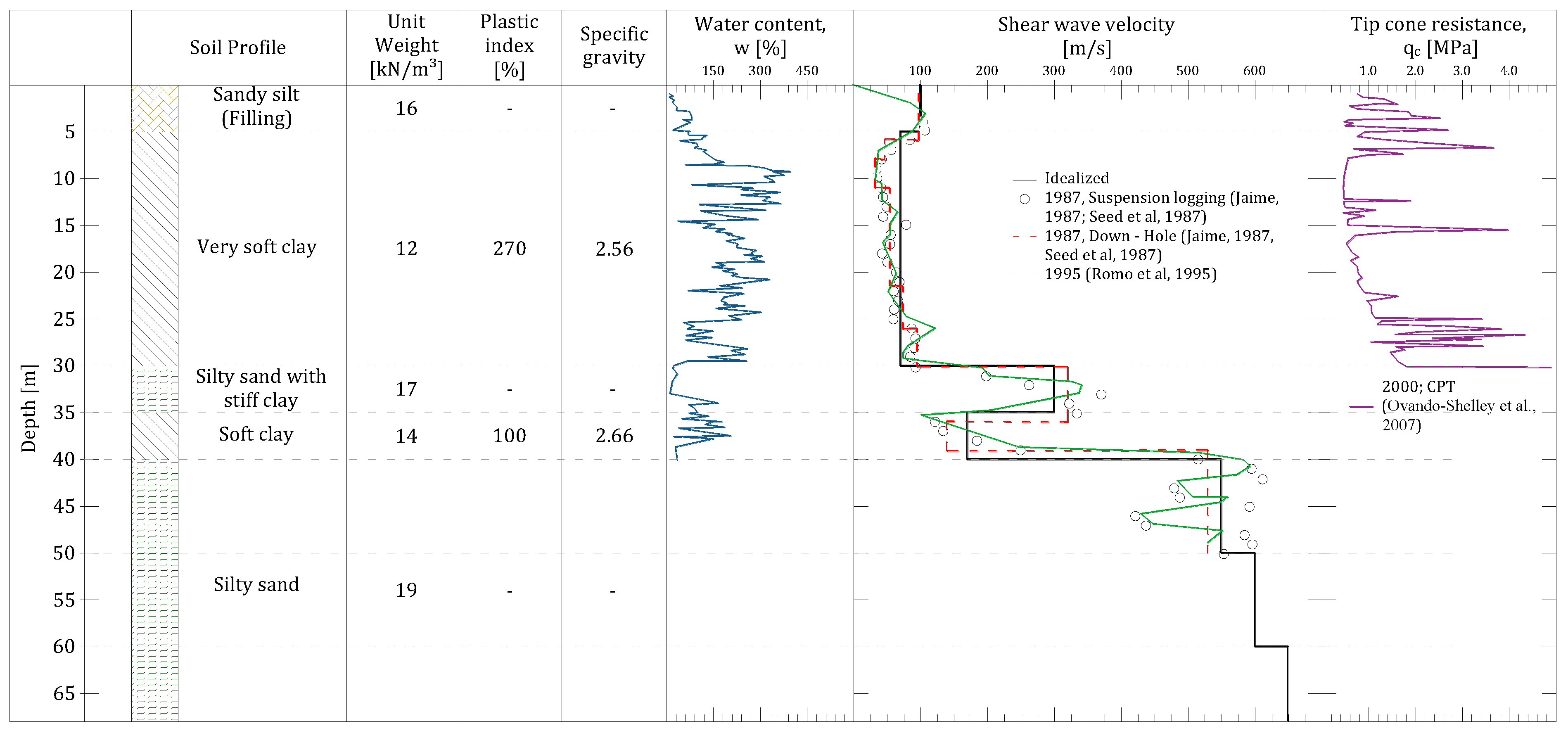
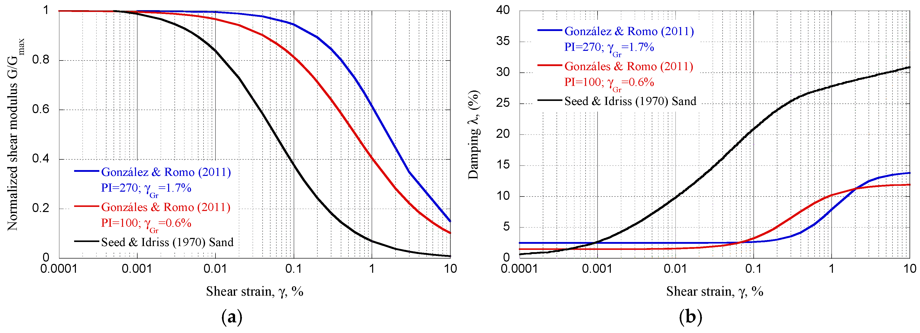
2.1. Soil Profile and Dynamic Properties
2.2. Building Features
- mass of each floor.
- stiffness of each floor.

| Stories | Basements Levels | Estimation for Stiff Buildings (s) | Estimation for Flexible Buildings (s) | Te Calculated Using Expression 1 (s) | Height (m) |
|---|---|---|---|---|---|
| 7 | 2 | 0.7 | 1.4 | 1.01 | 21.0 |
2.3. Tunnel Description
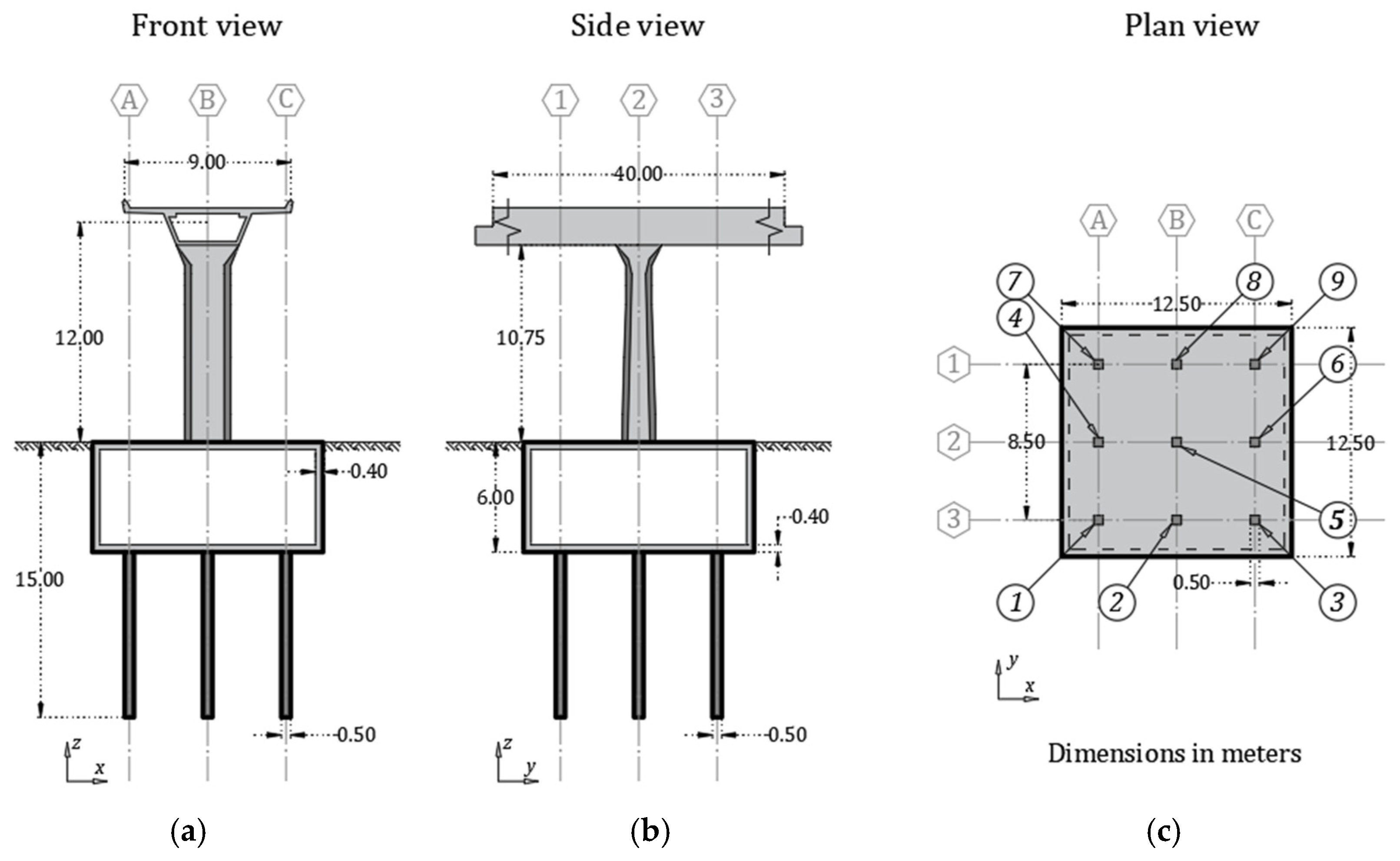
2.4. Urban Bridge Description
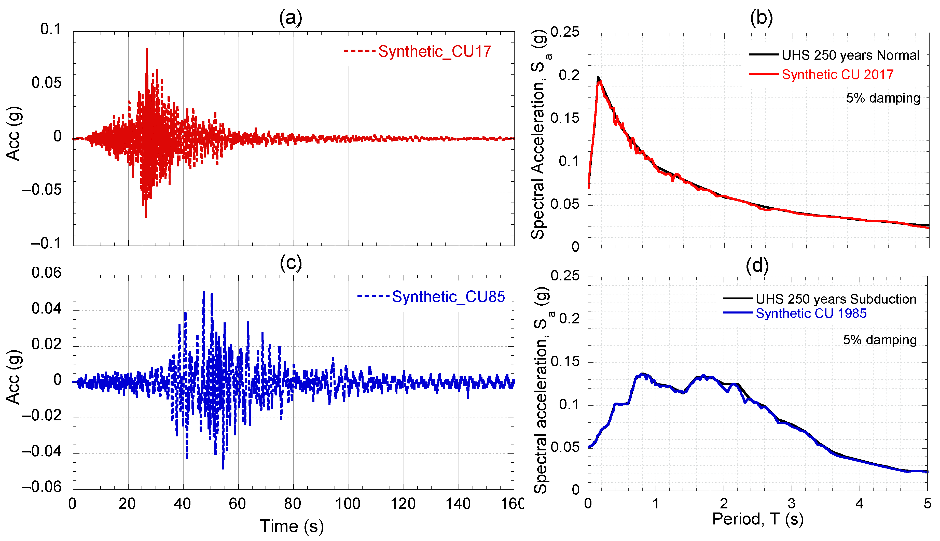
3. Seismic Environment Characterization
Site Response Analyses
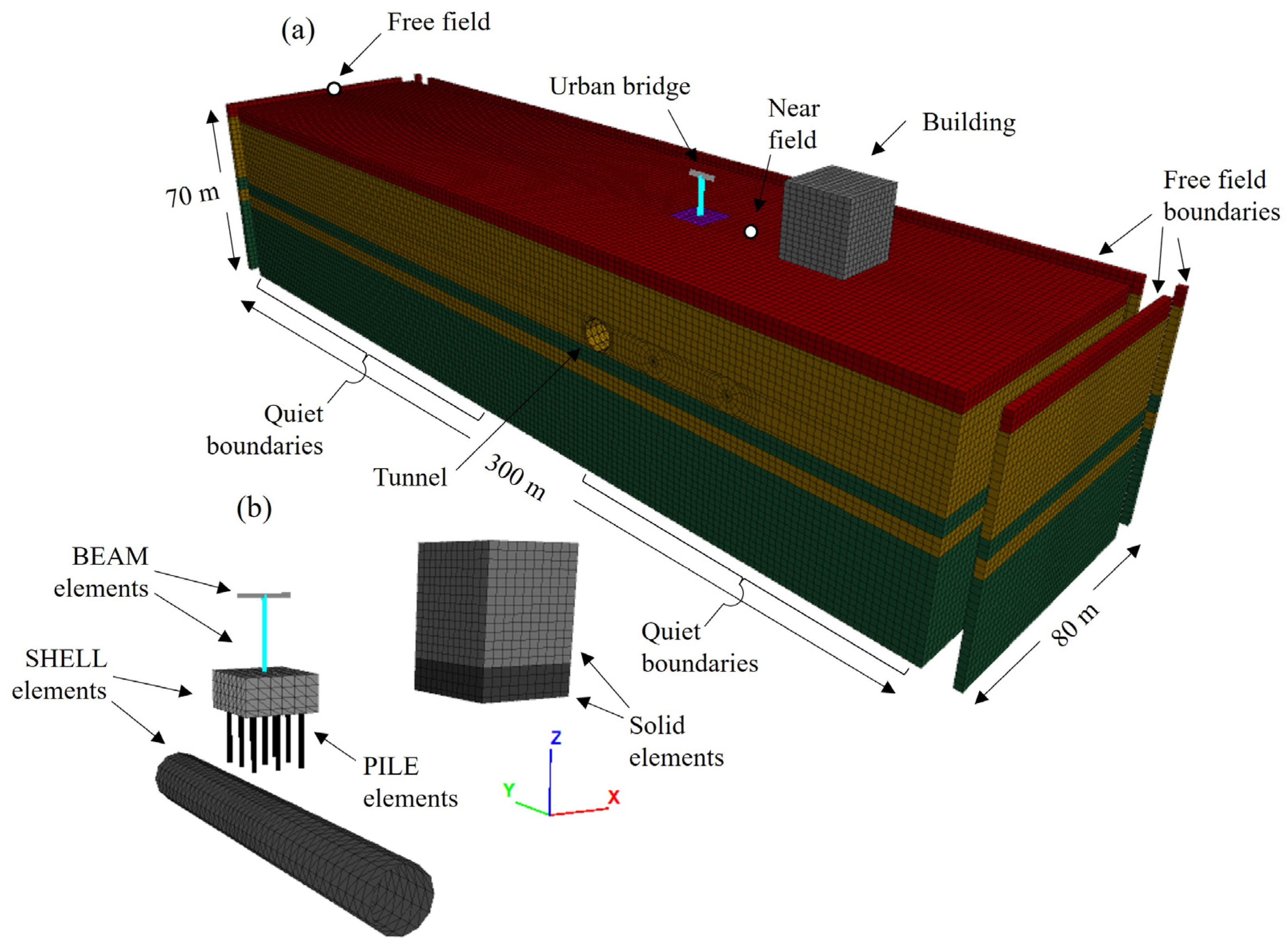
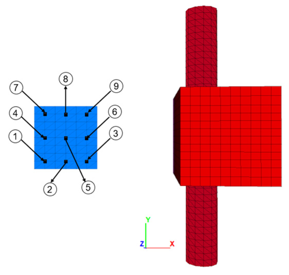
4. Numerical Model
- normalized secant modulus.
- logarithmic strain defined as .
- , , and = fitting curve parameters used by the sig3 model, to be matched with the modulus degradation curves.
- = the value of this parameter depends on the condition of the pile surface. For the rough surface (like the cast-in situ pile), it is suggested to be equal to 1 [43].
- and = cohesion and internal friction angle of the soil adjacent to the pile.
- = exposed perimeter of the pile.
- and = bulk and shear moduli of the soil adjacent to the pile.
- = smallest width of an adjoining zone in the normal direction.
- = pile diameter.
- and = cohesion and frictional strength components of the shear springs.
- , and = cohesion, frictional, and tensional strength components of the normal springs.
- and = stiffness of the shear and normal springs.
| Soil | (kN/m) | (°) | (MPa) | (kN/m) | (°) | (MPa) |
|---|---|---|---|---|---|---|
| Very soft clay | 60 | 0.1 | 1077 | 180 | 0.1 | 270 |
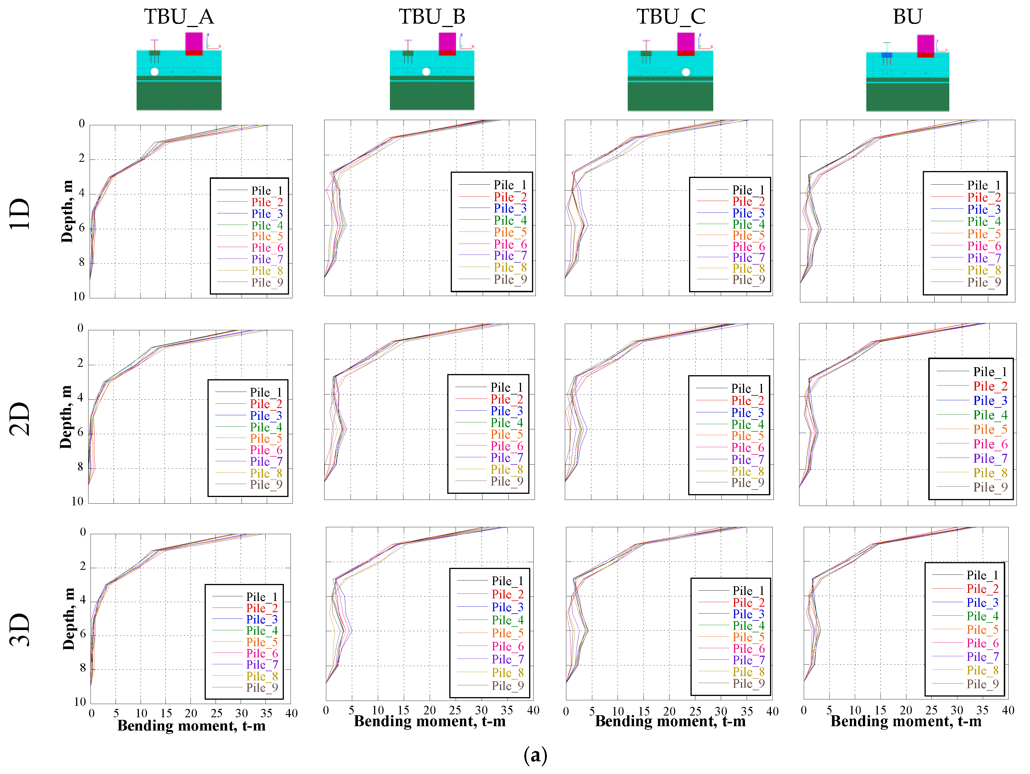
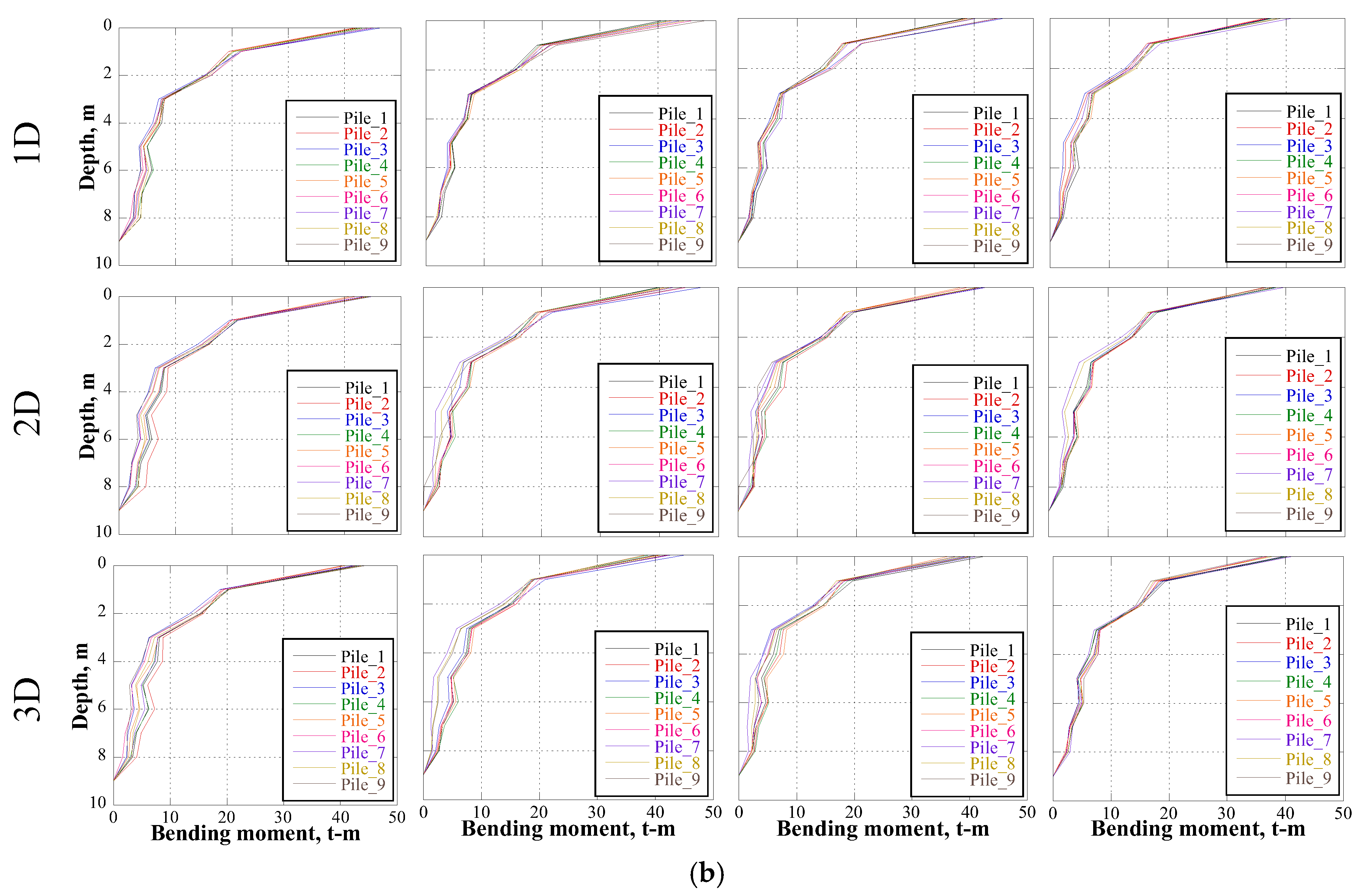
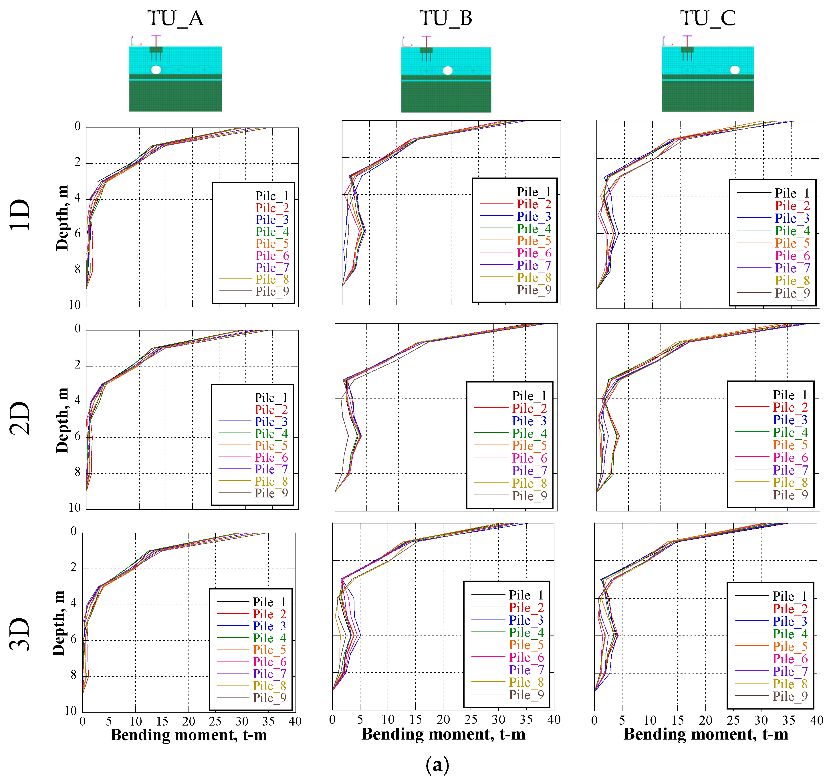
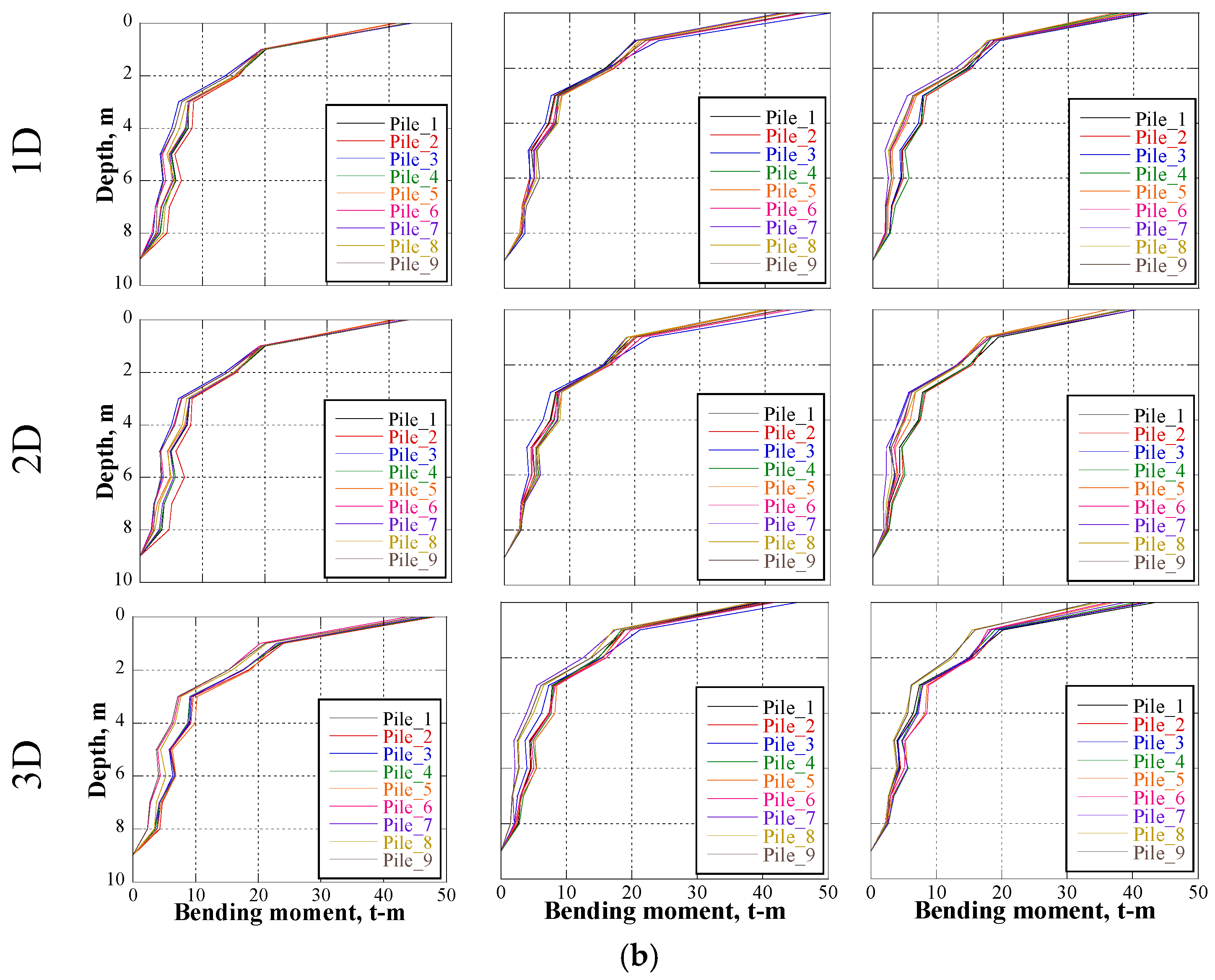
5. Seismic Tunnel–Bridge–Building Interaction
6. Conclusions
Author Contributions
Funding
Institutional Review Board Statement
Informed Consent Statement
Data Availability Statement
Conflicts of Interest
References
- Vicente, R.; Ferreira, T.; Maio, R. Seismic Risk at the Urban Scale: Assessment, Mapping and Planning. Procedia Econ. Financ. 2014, 18, 71–80. [Google Scholar] [CrossRef]
- Kappos, A.; Sextos, A.; Stefanidou, S.; Mylonakis, G.; Pitsiava, M.; Sergiadis, G. Seismic Risk of Inter-Urban Transportation Networks. Procedia Econ. Financ. 2014, 18, 263–270. [Google Scholar] [CrossRef]
- Argyroudis, S.A.; Mitoulis, S.; Winter, M.G.; Kaynia, A.M. Fragility of Transport Assets Exposed to Multiple Hazards: State-of-the-Art Review toward Infrastructural Resilience. Reliab. Eng. Syst. Saf. 2019, 191, 106567. [Google Scholar] [CrossRef]
- Argyroudis, S.A.; Mitoulis, S.A.; Hofer, L.; Zanini, M.A.; Tubaldi, E.; Frangopol, D.M. Resilience Assessment Framework for Critical Infrastructure in a Multi-Hazard Environment: Case Study on Transport Assets. Sci. Total Environ. 2020, 714, 136854. [Google Scholar] [CrossRef] [PubMed]
- Li, Y.; Tian, Y.; Zong, J. Shaking Table Test on Seismic Response of Tunnel-Soil Surface Structure System Considering Soil-Structure Interaction. Shock. Vib. 2022, 2022, 7515830. [Google Scholar] [CrossRef]
- Tian, Y.; Chen, S.; Liu, S.; Lu, X. Influence of Tall Buildings on City-Scale Seismic Response Analysis: A Case Study of Shanghai CBD. Soil Dyn. Earthq. Eng. 2023, 173, 108063. [Google Scholar] [CrossRef]
- Kato, B.; Wang, G. Regional Seismic Responses of Shallow Basins Incorporating Site-City Interaction Analyses on High-Rise Building Clusters. Earthq. Eng. Struct. Dyn. 2021, 50, 214–236. [Google Scholar] [CrossRef]
- Mayoral, J.M.; Mosqueda, G. Foundation Enhancement for Reducing Tunnel-Building Seismic Interaction on Soft Clay. Tunn. Undergr. Space Technol. 2021, 115, 104016. [Google Scholar] [CrossRef]
- Wang, G.; Lin, Y.; Wang, J.; Ma, C.; Liu, Z. Seismic Response Analysis of Twin Tunnels Parallelly Underpassing Station. Soil Dyn. Earthq. Eng. 2025, 192, 109310. [Google Scholar] [CrossRef]
- Edirisinghe, T.L.; Talbot, J.P. The Significance of Soil–Structure Interaction in the Response of Buildings to Ground-Borne Vibration from Underground Railways. J. Sound. Vib. 2025, 597, 118812. [Google Scholar] [CrossRef]
- Wang, G.; Yuan, M.; Miao, Y.; Wu, J.; Wang, Y. Experimental Study on Seismic Response of Underground Tunnel-Soil-Surface Structure Interaction System. Tunn. Undergr. Space Technol. 2018, 76, 145–159. [Google Scholar] [CrossRef]
- Hashash, Y.M.A.; Dashti, S.; Musgrove, M.; Gillis, K.; Walker, M.; Ellison, K.; Basarah, Y.I. Influence of Tall Buildings on Seismic Response of Shallow Underground Structures. J. Geotech. Geoenviron. Eng. 2018, 144, 04018097. [Google Scholar] [CrossRef]
- Mayoral, J.M.; Alcaraz, M.; Tepalcapa, S. Seismic Performance of Soil–Tunnel–Building Systems in Stiff Soils. Earthq. Spectra 2023, 39, 1214–1239. [Google Scholar] [CrossRef]
- Liu, B.; Zhang, D.; Li, X.; Li, J. Seismic Response of Underground Structure–Soil–Aboveground Structure Coupling System: Current Status and Future Prospects. Tunn. Undergr. Space Technol. 2022, 122, 104372. [Google Scholar] [CrossRef]
- Vicencio, F.; Alexander, N.A. Dynamic Structure-Soil-Structure Interaction in Unsymmetrical Plan Buildings Due to Seismic Excitation. Soil. Dyn. Earthq. Eng. 2019, 127, 105817. [Google Scholar] [CrossRef]
- Vicencio, F.; Alexander, N.A. Seismic Evaluation of Site-City Interaction Effects between City Blocks. Front. Built Environ. 2024, 10, 1403642. [Google Scholar] [CrossRef]
- Chávez-García, F.J.; Cárdenas-Soto, M. The Contribution of the Built Environment to the ‘Free-Field’ Ground Motion in Mexico City. Soil Dyn. Earthq. Eng. 2002, 22, 773–780. [Google Scholar] [CrossRef]
- Guéguen, P.; Colombi, A. Experimental and Numerical Evidence of the Clustering Effect of Structures on Their Response during an Earthquake: A Case Study of Three Identical Towers in the City of Grenoble, France. Bull. Seismol. Soc. Am. 2016, 106, 2855–2864. [Google Scholar] [CrossRef]
- Kham, M.; Semblat, J.F.; Bard, P.Y.; Dangla, P. Seismic Site-City Interaction: Main Governing Phenomena through Simplified Numerical Models. Bull. Seismol. Soc. Am. 2006, 96, 1934–1951. [Google Scholar] [CrossRef]
- Wirgin, A.; Bard, P.-Y. Effects of Buildings on the Duration and Amplitude of Ground Motion in Mexico City. Bull. Seismol. Soc. Am. 1996, 86, 914–920. [Google Scholar] [CrossRef]
- Guéguen, P.; Bard, P.-Y.; Chávez-García, F.J. Site-City Seismic Interaction in Mexico City-Like Environments: An Analytical Study. Bull. Seismol. Soc. Am. 2002, 92, 794–811. [Google Scholar] [CrossRef]
- Mayoral, J.M.; Mosqueda, G. Seismic Interaction of Tunnel-Building Systems on Soft Clay. Soil Dyn. Earthq. Eng. 2020, 139, 106419. [Google Scholar] [CrossRef]
- Seed, H.B.; Romo, M.P.; Sun, J.I.; Jaime, A.; Lysmer, J. The Mexico Earthquake of September 19, 1985—Relationships between Soil Conditions and Earthquake Ground Motions. Earthq. Spectra 1987, 4, 687–729. [Google Scholar] [CrossRef]
- Romo, M.P. Clay Behavior, Ground Response and Soil-Structure Interaction Studies. In Proceedings of the Third International Conference on Recent Advances in Geotechnical Engineering and Soil Dynamics, St. Louis, MO, USA, 2–7 April 1995; Volume II, pp. 1039–1051. [Google Scholar]
- Ovando-Shelley, E.; Ossa, A.; Romo, M.P. The Sinking of Mexico City: Its Effects on Soil Properties and Seismic Response. Soil Dyn. Earthq. Eng. 2007, 27, 333–343. [Google Scholar] [CrossRef]
- Jaime, A.; Romo, M.P.; Ovando-Shelley, E. Características Del Sitio SCT; Internal Report; IIUNAM: Mexico City, Mexico, 1987. [Google Scholar]
- Darendeli, M.B. Development of a New Family of Normalized Modulus Reduction and Material Damping Curves. Ph.D. Thesis, University of Texas at Austin, Austin, TX, USA, 2001. [Google Scholar]
- González, C.M.B.; Romo, M.P.O. Estimación de propiedades dinámicas de arcillas. Rev. Ing. Sísmica 2011, 84, 1–23. [Google Scholar] [CrossRef]
- Seed, H.; Idriss, I.M. Soil Moduli and Damping Factors for Dynamic Response Analyses; Report EERRC-70-10; University of California: Berkeley, CA, USA, 1970. [Google Scholar]
- Franke, K.W.; Candia, G.; Mayoral, J.M.; Wood, C.M.; Montgomery, J.; Hutchinson, T.; Morales-Velez, A.C. Observed Building Damage Patterns and Foundation Performance in Mexico City Following the 2017 M7.1 Puebla-Mexico City Earthquake. Soil Dyn. Earthq. Eng. 2019, 125, 105708. [Google Scholar] [CrossRef]
- Romo, M.P.; Bárcena, A. Análisis de la Interacción Dinámica Suelo-Estructura en la Ciudad de México; IIUNAM Series 565; IIUNAM: Mexico City, Mexico, 1994. [Google Scholar]
- Mayoral, J.M.; Pérez, M.; Roman, A. Integrated Geoenvironmental Models for Performance Assessment of Tunnels in Soft Soils. J. Perform. Constr. Facil. 2025; in press. [Google Scholar]
- Muría-Vila, D.; Sánchez-Ramírez, A.R.; Huerta-Carpizo, C.H.; Aguilar, G.; Pérez, J.C.; Carrillo Cruz, R.E. Field Tests of Elevated Viaducts in Mexico City. J. Struct. Eng. 2015, 141, D4014001. [Google Scholar] [CrossRef]
- Mayoral, J.M.; Romo, M.P. Seismic Response of Bridges with Massive Foundations. Soil. Dyn. Earthq. Eng. 2015, 71, 88–99. [Google Scholar] [CrossRef]
- Mayoral, J.M.; Asimaki, D.; Tepalcapa, S.; Wood, C.; Roman-de la Sancha, A.; Hutchinson, T.; Franke, K.; Montalva, G. Site Effects in Mexico City Basin: Past and Present. Soil. Dyn. Earthq. Eng. 2019, 121, 369–382. [Google Scholar] [CrossRef]
- Auvinet, G. Seismic Response of Subsoil and Building Foundations in Mexico City (1985–2017). In Proceedings of the ISSMGE Touring Lecture, Mexico City, Mexico, 19 November 2018. [Google Scholar]
- Heresi, P.; Ruiz-García, J.; Payán-Serrano, O.; Miranda, E. Observations of Rayleigh Waves in Mexico City Valley during the 19 September 2017 Puebla–Morelos, Mexico Earthquake. Earthq. Spectra 2020, 36, 62–82. [Google Scholar] [CrossRef]
- Singh, S.K.; Cruz-Atienza, V.; Pérez-Campos, X.; Iglesias, A.; Hjörleifsdóttir, V.; Reinoso, E.; Ordaz, M.; Arroyo, D. Deadly Intraslab Mexico Earthquake of 19 September 2017 (Mw 7.1): Ground Motion and Damage Pattern in Mexico City. Seismol. Res. Lett. 2018, 89, 2193–2203. [Google Scholar] [CrossRef]
- RCDF Reglamento de Construcciones Para El Distrito Federal; Administracion Publica Del Distrito Federal, Jefatura de Gobierno, Normas Técnicas Complementarias Para Diseño Por Sismo: Mexico City, Mexico, 2023.
- Lilhanand, K.; Tseng, W.S. Development and Application of Realistic Earthquake Time Histories Compatible with Multiple Damping Response Spectra. Proc. Ninth World Conf. Earthq. Eng. 1988, 2, 819–824. [Google Scholar]
- Alatik, L.; Abrahamson, N. An Improved Method for Nonstationary Spectral Matching. Earthq. Spectra 2010, 26, 601–617. [Google Scholar] [CrossRef]
- Schnabel, P.B.; Lysmer, J.; Seed, H.B. SHAKE: A Computer Program for Earthquake Response Analysis of Horizontally Layered Sites; Report No. EERC 72-12; Earthquake Engineering Research Center, University of California: Berkeley, CA, USA, 1972. [Google Scholar]
- Itasca Consulting Group. FLAC3D: Fast Lagrangian Analysis of Continua in 3 Dimensions; User’s Guide; Itasca Consulting Group, Inc.: Minneapolis, MN, USA, 2019. [Google Scholar]
- Lysmer, J.; Kuhlemeyer, R.L. Finite Dynamic Model for Infinite Media. J. Eng. Mech. Div. 1969, 95, 859–877. [Google Scholar] [CrossRef]
- Yeganeh, N.; Bolouri Bazaz, J.; Akhtarpour, A. Seismic Analysis of the Soil-Structure Interaction for a High Rise Building Adjacent to Deep Excavation. Soil Dyn. Earthq. Eng. 2015, 79, 149–170. [Google Scholar] [CrossRef]
- Kramer, S.L.; Stewart, J.P. Geotechnical Earthquake Engineering, 2nd ed.; CRC Press: Boca Raton, FL, USA, 2024; ISBN 9781003512011. [Google Scholar]
- Isari, M.; Razavi, S.K.; Tarinejad, R.; Sobhkhiz Foumani, R. Investigating the Effects of Underground Structures on the Scattering of Seismic Waves Reaching the Ground Surface. Transp. Infrastruct. Geotechnol. 2022, 9, 321–337. [Google Scholar] [CrossRef]
- Jing, G.U.O.; Jianyun, C.; Liu, Y.U. Influence of Tunnel on Inter-Story Drift of Adjacent Structures. Chin. J. Undergr. Space Eng. 2017, 13, 765–772. [Google Scholar]
- Guo, J.; Chen, J.; Bobet, A. Influence of a Subway Station on the Inter-Story Drift Ratio of Adjacent Surface Structures. Tunn. Undergr. Space Technol. 2013, 35, 8–19. [Google Scholar] [CrossRef]
- Vicencio, F.; Alexander, N.A.; Saavedra Flores, E.I. A State-of-the-Art Review on Structure-Soil-Structure Interaction (SSSI) and Site-City Interactions (SCI). Structures 2023, 56, 105002. [Google Scholar] [CrossRef]
- Vicencio, F.; Alexander, N.A. Dynamic Interaction between Adjacent Buildings through Nonlinear Soil during Earthquakes. Soil Dyn. Earthq. Eng. 2018, 108, 130–141. [Google Scholar] [CrossRef]
- Rabeti Moghadam, M.; Baziar, M.H. Seismic Ground Motion Amplification Pattern Induced by a Subway Tunnel: Shaking Table Testing and Numerical Simulation. Soil Dyn. Earthq. Eng. 2016, 83, 81–97. [Google Scholar] [CrossRef]


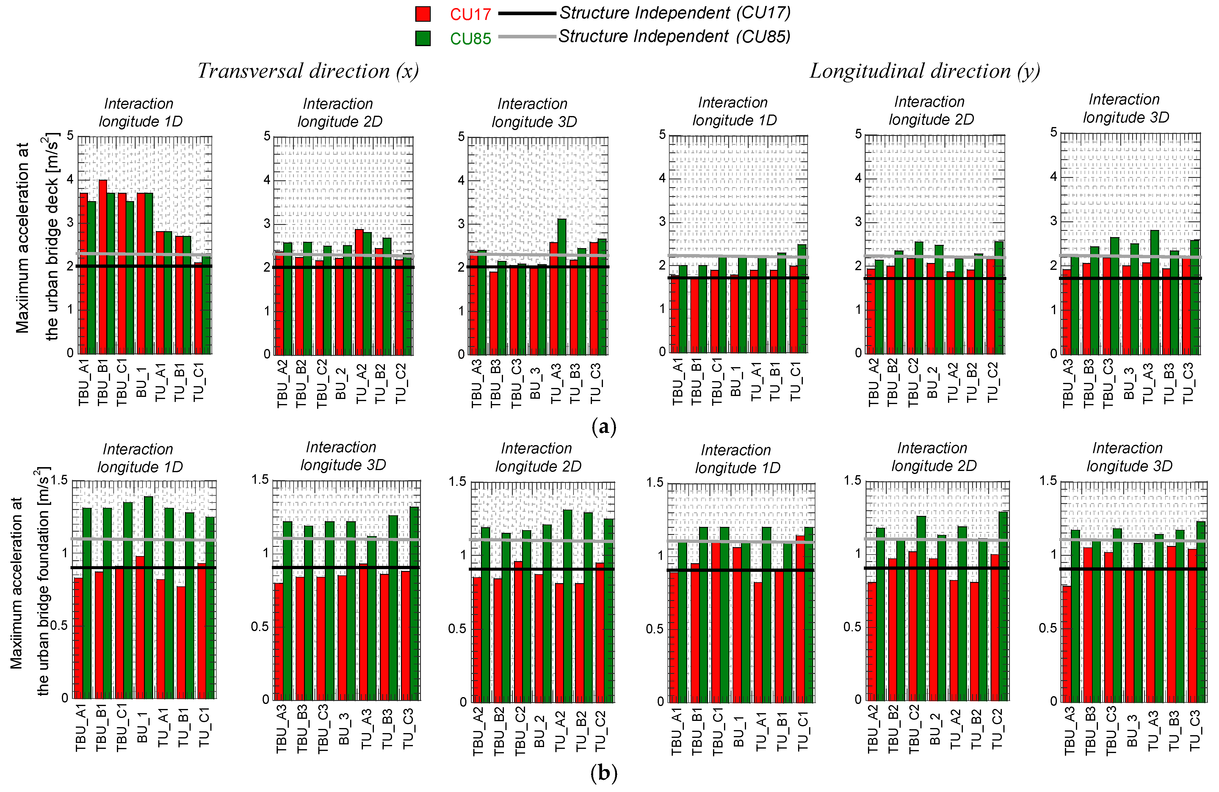
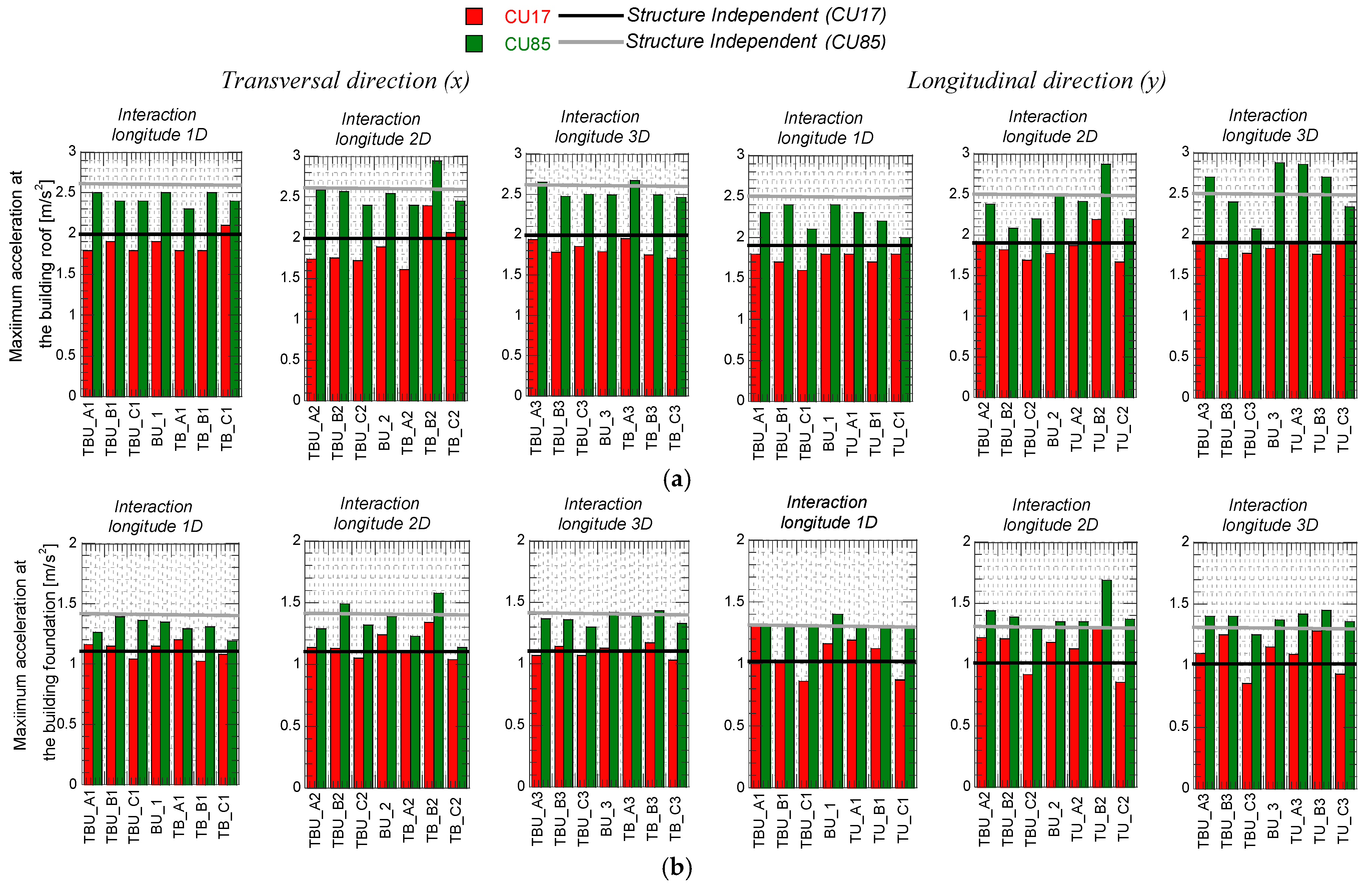
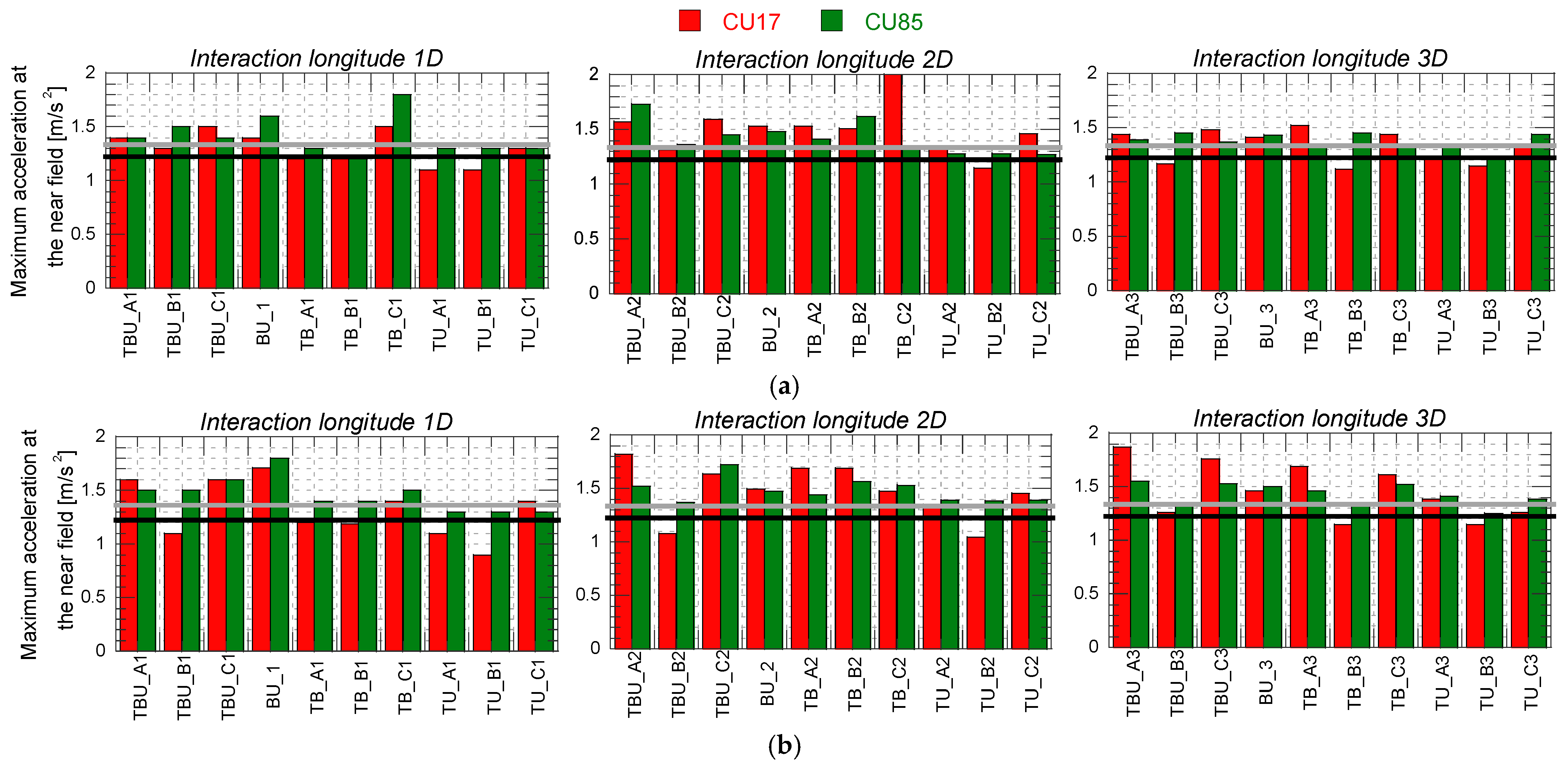
| Interaction Longitude (Diameters) | Position of the Tunnel for the Tunnel–Building–Bridge Scenarios | Position of the Tunnel for the Tunnel–Bridge Scenarios | Position of the Tunnel for the Tunnel–Building Scenarios | Building–Bridge Without Tunnel | ||||||
|---|---|---|---|---|---|---|---|---|---|---|
| A | B | C | A | B | C | A | B | C | ||
| 1 | TBU_A1 | TBU_B1 | TBU_C1 | TU_A1 | TU_B1 | TU_C1 | TB_A1 | TB_B1 | TB_C1 | BU_1 |
| 2 | TBU_A2 | TBU_B2 | TBU_C2 | TU_A2 | TU_B2 | TU_C2 | TB_A2 | TB_B2 | TB_C2 | BU_2 |
| 3 | TBU_A3 | TBU_B3 | TBU_C3 | TU_A3 | TU_B3 | TU_C3 | TB_A3 | TB_B3 | TB_C3 | BU_3 |
| Direction | Structural Period (s) |
|---|---|
| Transversal | 0.45 |
| Longitudinal | 0.60 |
| Seismogenic Zone | Earthquake Name | Year | Mw, Moment Magnitude | PGA, Peak Ground Acceleration (g) | TD (s) | Frequency Content (Hz) | Arias Intensity (cm/s) |
|---|---|---|---|---|---|---|---|
| Intraplate | Puebla, Mexico, CU17 | 2017 | 7.1 | 0.059 | 29.6 | 0.23 to 3.5 | 12.7 |
| Interface | Michoacan, Mexico, CU85 | 1985 | 8.1 | 0.033 | 49.7 | 0.38 to 1.36 | 15.5 |
| Strata | Mohr–Coulomb Properties | Elastic Properties | Sig3 Hysteretic Model | Estimated Level of Nonlinearity | |||||||
|---|---|---|---|---|---|---|---|---|---|---|---|
| γ (kN/m3) | c (kPa) | φ (°) | Gmax (GPa) | ν | a | B | x0 | γ (%) | G/Gmax | λ (%) | |
| Sandy silt | 16.0 | 30 | 35 | 12.0 | 0.30 | 1.014 | −0.480 | −0.600 | 0.01–0.15 | 0.4–0.9 | 9–21 |
| Very soft clay | 12.0 | 40 | 0 | 5.6 | 0.45 | 1.000 | −0.460 | 0.320 | 0.13–0.69 | 0.8–0.95 | 3–4 |
| Silty sand with stiff clay | 17.0 | 15 | 27 | 126.0 | 0.30 | 1.014 | −0.480 | −1.250 | 0.02–0.04 | 0.7–0.8 | 11–14 |
| Soft clay | 14.0 | 80 | 0 | 34.7 | 0.45 | 1.000 | −0.490 | −0.020 | 0.01–0.11 | 0.85–1.0 | 2–3 |
| Silty sand | 19.0 | 15 | 40 | 390 to 613 | 0.28 | 1.014 | −0.550 | −1.500 | 0.01–0.02 | 0.8–0.9 | 5–6 |
Disclaimer/Publisher’s Note: The statements, opinions and data contained in all publications are solely those of the individual author(s) and contributor(s) and not of MDPI and/or the editor(s). MDPI and/or the editor(s) disclaim responsibility for any injury to people or property resulting from any ideas, methods, instructions or products referred to in the content. |
© 2025 by the authors. Licensee MDPI, Basel, Switzerland. This article is an open access article distributed under the terms and conditions of the Creative Commons Attribution (CC BY) license (https://creativecommons.org/licenses/by/4.0/).
Share and Cite
Mayoral, J.M.; Pérez, M.; Román-de la Sancha, A.; Rosas, J. Seismic Performance of Modal Transfer Stations on Soft Clays. Appl. Sci. 2025, 15, 3406. https://doi.org/10.3390/app15063406
Mayoral JM, Pérez M, Román-de la Sancha A, Rosas J. Seismic Performance of Modal Transfer Stations on Soft Clays. Applied Sciences. 2025; 15(6):3406. https://doi.org/10.3390/app15063406
Chicago/Turabian StyleMayoral, Juan Manuel, Mauricio Pérez, Azucena Román-de la Sancha, and Jimena Rosas. 2025. "Seismic Performance of Modal Transfer Stations on Soft Clays" Applied Sciences 15, no. 6: 3406. https://doi.org/10.3390/app15063406
APA StyleMayoral, J. M., Pérez, M., Román-de la Sancha, A., & Rosas, J. (2025). Seismic Performance of Modal Transfer Stations on Soft Clays. Applied Sciences, 15(6), 3406. https://doi.org/10.3390/app15063406