An Over-Deterministic Method for Mode III SIF Calculation Using Full-Field Experimental Displacement Fields

Abstract

The paper proposes and tests an approach to determine the stress intensity factors (SIF) of cracks subjected to mode III using full-field displacements as opposed to the crack opening displacement (COD) method, which uses only two data points. The proposed scheme fits displacement data into Williams’ series for cracks, solving the equations using the over-deterministic Least Squares Method (LSM). The method is tested in tubes with through-cracks under axial and cyclic torque loading, and both proportional and non-proportional loading. The Digital Image Correlation (DIC) technique measured the displacement fields, and an approach is presented to address the curvature error in the tube samples. The experimentally determined SIF and SIF ranges with the proposed method are compared with respective values found using COD equations showing a pronounced nonlinear variation. It is concluded that for most, both methods agree, and for the LSM, the number of expansion terms in Williams’ series seems to make no difference, exhibiting less noisy results than the COD method and effectively addresses nonlinear variations in SIF calculations across different loading conditions, ultimately enhancing the understanding of crack behavior under mode III loading.

1. Introduction

The importance of mode III in crack displacement has been extensively documented in the literature [1,2,3,4,5,6,7] and its consequence in cylindrical components [8]. Literature results demonstrated [2,4,9,10] that out-of-plane displacements are present, even when direct out-of-plane loading is not applied, generating a crack driving force in the out-of-plane direction. Furthermore, Sapora [11] recently noted the lack of literature dedicated to mode III. Ju et al. [12] found that including mode III (along with Poisson’s ratio and T-stress) enhanced crack initiation prediction. SIFs can be calculated from displacements obtained through numerical simulation (such as XFEM or DBEM) using weight functions, virtual crack (VCC), J, or the interaction integral technique from a geometric factor (using ASTM or SIF manuals).

From data acquired through experimental methods, clip gauges are known for their reliable measures and low cost, but in the case of kinked cracks, the displacements given by the COD gauge may not adequately describe the stress field on the crack tip. However, at the time of writing this paper, there are no clip gauges that can simultaneously measure the crack’s opening and sliding displacements. One would require clip gauges in addition to a second technique, like strain gauge or extensometers. Nevertheless, one would require separate setups for opening and sliding. The digital image correlation (DIC) technique provides independent full-field displacement measurements in 2D or 3D with the use of two or more cameras. Even for a larger budget, it has become standard equipment in many laboratories. Therefore, such kinds of readings are readily available. Therefore, one can use such experimental measurements and fit them to a stress function; the J integral is a robust method to calculate SIF [13], but one needs to establish strain and stresses before using it, and the VCC is preferred for delamination prediction. Additionally, one needs a method to decompose the J integral values as it gives the total energy used to create a new surface crack regardless of direction [13]. Moreover, despite results demonstrating that mode III displacements appear even when no direct out-plane-loading is applied, there is no robust method to calculate SIF mode III using full-field experimental displacements. Therefore, disregarding mode III can lead to lower equivalent SIF [14], uncertainty in 3D crack initiation and propagation [5], or fracture toughness overestimation [15].

On the other hand, many schemas have been devised to produce mode III on sample coupons such as tubes and cylinders under torsion [7], rotated beams [16,17], inclined cracks [18,19,20], modified Brazilian disk [21,22], and modified Arcan [23] among others. A review of some testing fixtures for mode III can be found in [15,24]. Therefore, the importance that the community gives to testing samples under out-of-plane displacement can be seen. All these methods, along with full-field independent displacements, such as the ones provided with the DIC technique, create the need for a robust method to calculate SIF mode III. The paper shows a scheme to fit full-field displacement fields to Williams’ equations in mode III and how to solve them with the least squares method (LSM).

2. Literature Review

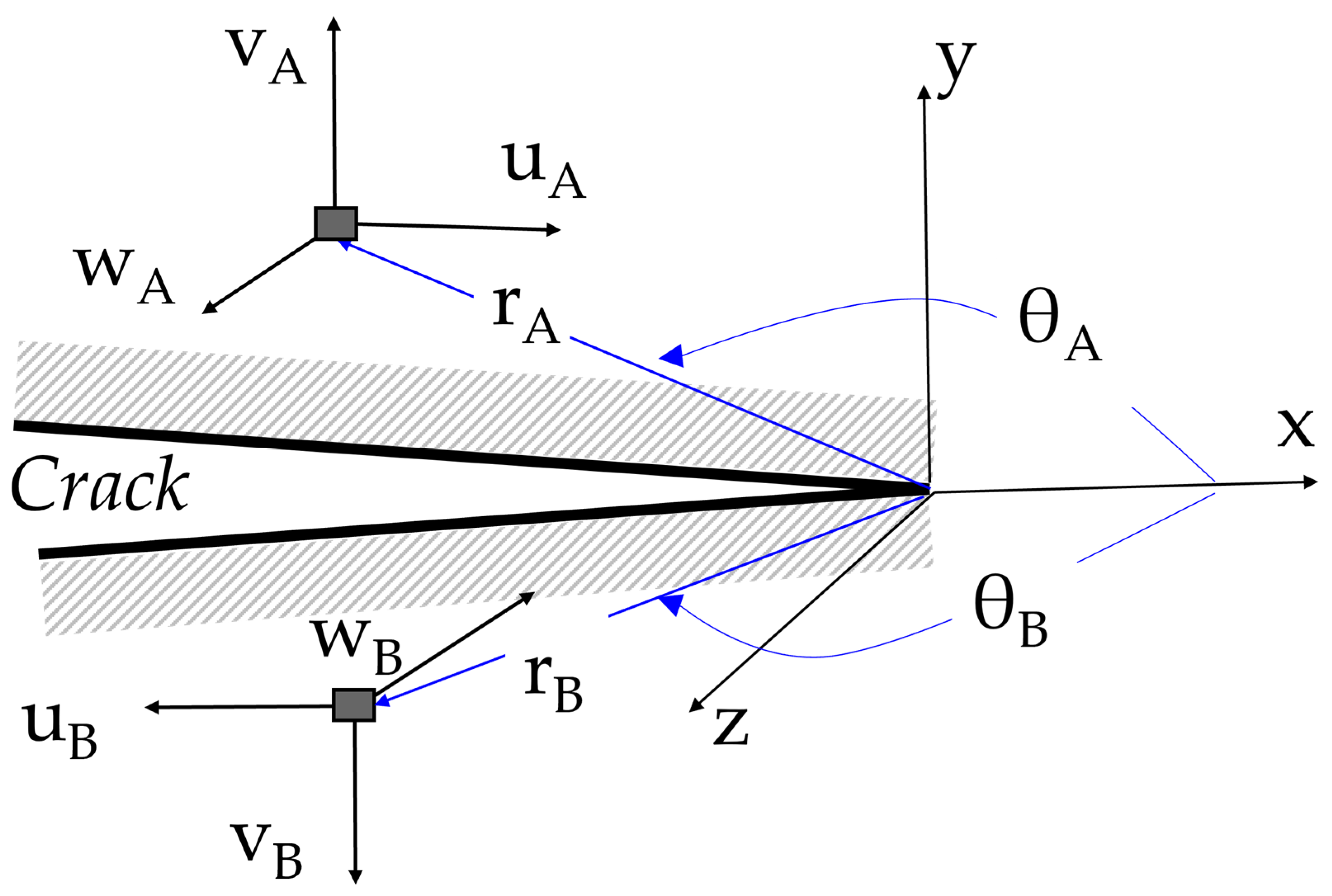
2.1. Theoretical Background

Cracks prefer to grow perpendicular to the normal stress direction. However, cracked structures subjected to multiaxial loading can display three fracture modes [12]: mode I (opening), mode II (in-plane shear), and mode III (out-of-plane shear), as shown in Figure 1. Most of the solutions for SIFs are numerical, with only a few analytical approaches, such as Williams’ series, based on a complex Airy stress function, as shown in Equation (1) [25], for an infinite cracked plate, as seen in Figure 1, with the coordinate system located at the crack tip. The independent displacements U, V, and W are represented as an infinite sequence of n terms. Polar coordinates (r, θ) describe the positions of the opposite-to-the-crack points A and B from the origin located at the crack tip.

$$\begin{array}{l}u={\displaystyle \sum _{n=1}^{\infty }\frac{r^{n/2}}{2G}}\left(\begin{array}{l}{a}_n\left\{\left[k+{\displaystyle \frac{n}{2}}+{(-1)}^n\right]Cos{\displaystyle \frac{n\theta }{2}}-{\displaystyle \frac{n}{2}}Cos\left({\displaystyle \frac{n-4}{2}}\right)\theta \right\}-\\ b_n\left\{\left[k+{\displaystyle \frac{n}{2}}-{(-1)}^n\right]Sin{\displaystyle \frac{n\theta }{2}}-{\displaystyle \frac{n}{2}}Sin\left({\displaystyle \frac{n-4}{2}}\right)\theta \right\}\end{array}\right)\\ v={\displaystyle \sum _{n=1}^{\infty }\frac{r^{n/2}}{2G}\left(\begin{array}{l}{a}_n\left\{\left[k-\frac{n}{2}+{(-1)}^n\right]Sin\frac{n\theta }{2}+\frac{n}{2}Sin\left(\frac{n-4}{2}\right)\theta \right\}+\\ b_n\left\{\left[k-\frac{n}{2}+{(-1)}^n\right]Cos\frac{n\theta }{2}+\frac{n}{2}Cos\left(\frac{n-4}{2}\right)\theta \right\}\end{array}\right)}\\ w={\displaystyle \sum _{n=1}^{\infty }\frac{2r^{n-\raisebox{1ex}{$1$}\!\left/ \!\raisebox{-1ex}{$2$}\right.}}{G}\left\{c_{n}Sin\left(n-\frac{1}{2}\right)\theta \right\}}\end{array}$$

(1)

where u is parallel-to-crack displacements, v is perpendicular-to-crack displacements, w is perpendicular-to-plane displacements, a₁ = K_I/√2π, b₁ = K_II/√2π, c₁ = K_III/√2π, a₂ = σ_ox/4, r and θ are the radius and angle of an arbitrary point, G is shear modulus, n is the numbers of terms in the expansion series, and k is the Kolosov constant given by Equation (2).

$$k=\{\begin{array}{c}3-4\nu ;{\epsilon }_{pl}\\ {\displaystyle \frac{3-\nu }{1+\nu }};{\sigma }_{pl}\end{array}$$

(2)

Using Equation (1), Zhang and He [26] computed SIF by expressing Williams’ displacement fields as Equation (3) using experimentally obtained mixed-mode data (I and II).

$$\begin{array}{l}u={\displaystyle \sum _{n=1}^N{a}_n}{f}_{In(r,\theta )}-{\displaystyle \sum _{n=1}^N{b}_n}{f}_{IIn(r,\theta )}+T_x-R{y}_n\\ v={\displaystyle \sum _{n=1}^N{a}_n}{g}_{In(r,\theta )}-{\displaystyle \sum _{n=1}^N{b}_n}{g}_{IIn(r,\theta )}+T_y+R{x}_n\end{array}$$

(3)

where N is the number of terms in Williams’ series, T_x and T_y are the rigid body components in x and y, respectively, and Ry_n and Rx_n are the rigid body rotation around X and Y, respectively. Equation (3) can be rewritten in matrix form, as shown in Equation (4), where [a(r, θ)] and [b(r, θ)] is a matrix made up of functions described in Equation (5) that are explained in Equation (6), {Δ} is the unknown vector coefficients of the displacement functions, and {h} is the concatenated vector of known displacements. The Least Squares Method (LSM) [27] can solve the resulting over-determined system. Furthermore, Ju and Chung [28] checked the accuracy of the LSM to calculate SIF. This over-deterministic method has been implemented, among others, for modes I and II [29].

$$\left\{h\right\}=\left[b\right]\{\Delta \}$$

(4)

$$h=\left[\begin{array}{c}{u}_1\\ ⋮\\ u_M\\ v_1\\ ⋮\\ v_M\end{array}\right];\Delta =\left[\begin{array}{c}{a}_1\\ ⋮\\ a_M\\ b_1\\ ⋮\\ b_M\end{array}\right];b=\left[\begin{array}{ccccccc}{f}_{I1(r1,\theta 1)}& \dots & f_{II1(r1,\theta 1)}& \dots & 1& 0& -y_1\\ ⋮& \ddots & ⋮& \ddots & ⋮& ⋮& ⋮\\ f_{IM(rM,\theta M)}& \dots & f_{IIM(rM,\theta M)}& \dots & 1& 0& -y_1\\ g_{I1(r1,\theta 1)}& \dots & g_{II1(r1,\theta 1)}& \dots & 0& 1& x_1\\ ⋮& \ddots & ⋮& \ddots & ⋮& ⋮& ⋮\\ g_{IM(rM,\theta M)}& \dots & g_{IIM(rM,\theta M)}& \dots & 0& 1& x_1\end{array}\right]$$

(5)

$$\begin{array}{c}{f}_{In(r,\theta )}={\displaystyle \frac{r^{n/2}}{2G}}\left[\left(k-{\displaystyle \frac{n}{2}}+{(-1)}^n\right)Cos{\displaystyle \frac{n\theta }{2}}-{\displaystyle \frac{n}{2}}Cos\theta \left({\displaystyle \frac{n}{2}}-2\right)\right]\\ f_{IIn(r,\theta )}={\displaystyle \frac{r^{n/2}}{2G}}\left[\left(k+{\displaystyle \frac{n}{2}}-{(-1)}^n\right)Sin{\displaystyle \frac{n\theta }{2}}-{\displaystyle \frac{n}{2}}Sin\theta \left({\displaystyle \frac{n}{2}}-2\right)\right]\\ g_{In(r,\theta )}={\displaystyle \frac{r^{n/2}}{2G}}\left[\left(k-{\displaystyle \frac{n}{2}}-{(-1)}^n\right)Sin{\displaystyle \frac{n\theta }{2}}+{\displaystyle \frac{n}{2}}Sin\theta \left({\displaystyle \frac{n}{2}}-2\right)\right]\\ g_{IIn(r,\theta )}={\displaystyle \frac{r^{n/2}}{2G}}\left[\left(-k+{\displaystyle \frac{n}{2}}-{(-1)}^n\right)Cos{\displaystyle \frac{n\theta }{2}}-{\displaystyle \frac{n}{2}}Cos\theta \left({\displaystyle \frac{n}{2}}-2\right)\right]\end{array}$$

(6)

Different methods have been used to experimentally calculate SIF in LEFM [6,13,25] in a single or a combination of modes. The importance of including mode III has been extensively acknowledged [3,7,16,24,30], whereas leaving it out may lead to prediction errors [14], impact crack length [31], or crack path prediction [5,32]. Langlois [33] combined X-FEM with a nested mesh to simulate III modes in curved crack fronts. In [12], K_III was calculated from the relative displacement of two points numerically calculated and compared to XFEM and experimental results, a similar approach used in [9]. Gómez et al. [31] discussed how toughness could be affected when there is mixed-mode loading, including mode III, and Kujawski [34] acknowledged the effect of plasticity in CP. So, unaccounted K_III values might lead to leaving out plasticity effects, which could potentially underestimate crack growth. Finally, Tavares and Castro [35] discussed the issues of several formulations for equivalent SIF but did not include mode III.

The J integral [13,36] is a viable alternative that is used in many commercial FEM software. However, in experimental work, it can be cumbersome to implement, and it also needs a mode separation method.

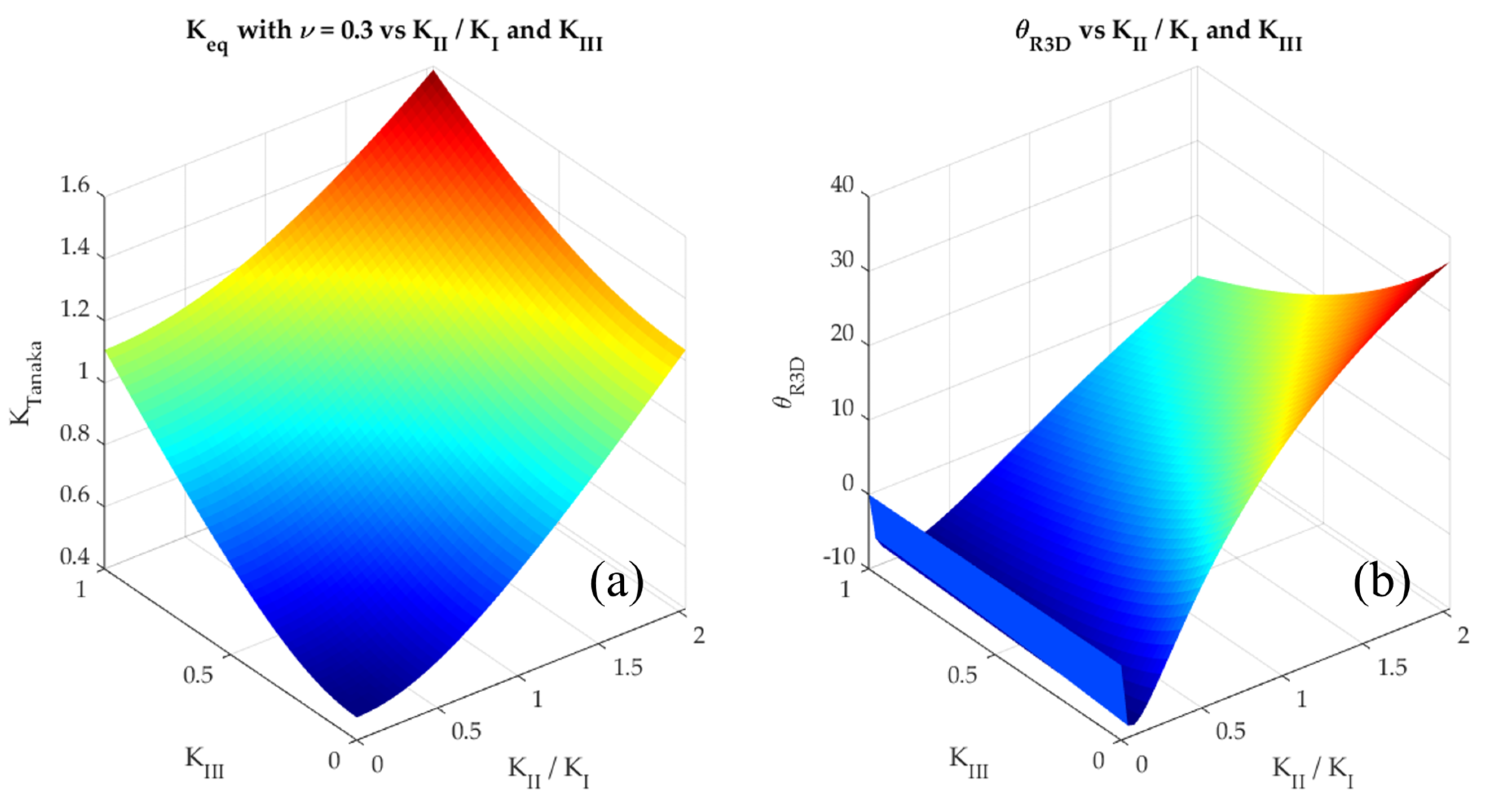
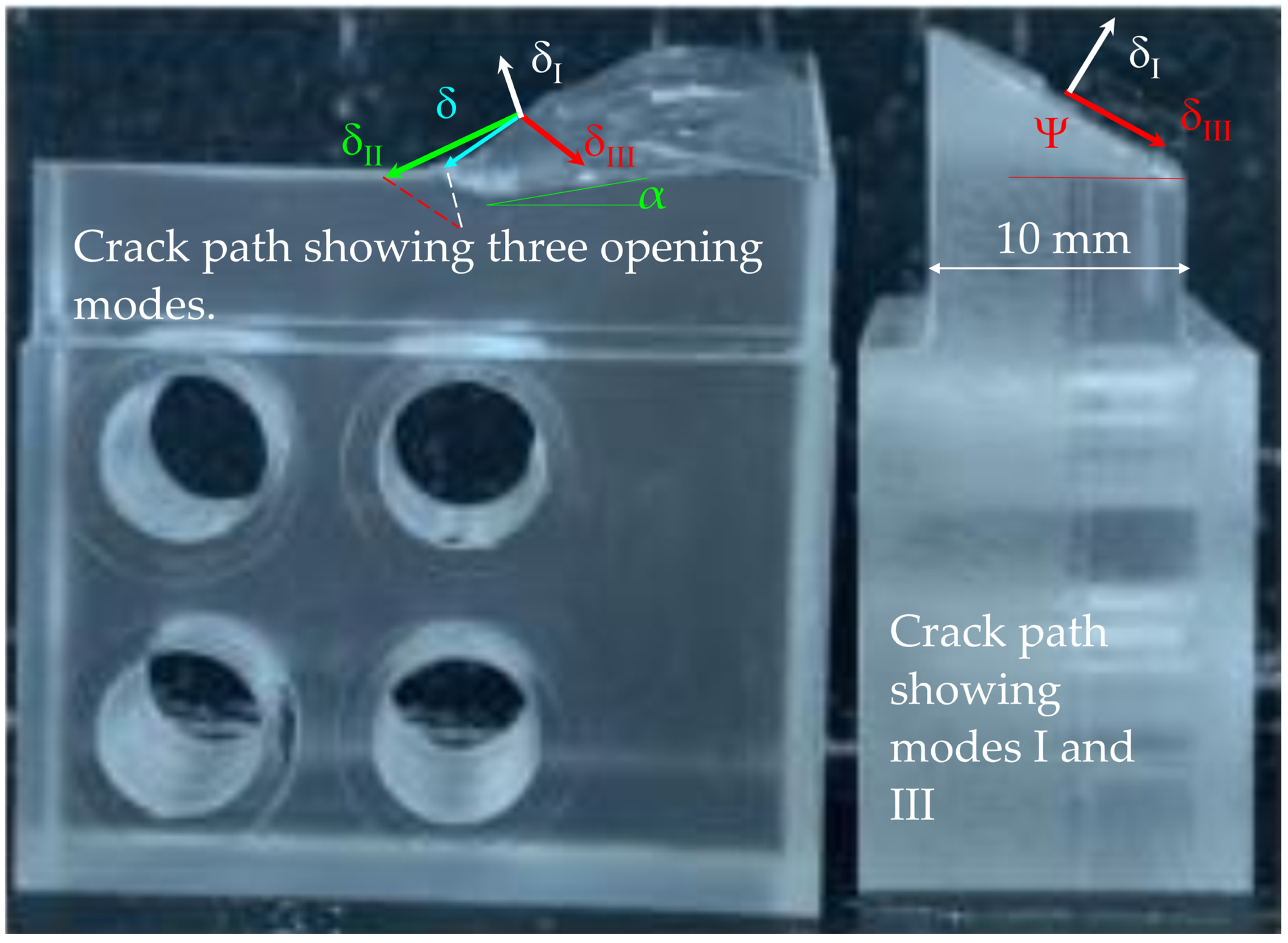
2.2. Plausible Effects of Ignoring K_III on CP and Keq

Ignoring mode III has an impact on the equivalent SIF (Keq) and the fracture path, according to theoretical models based on Westergaard’s stress function.

By representing displacement as vectors, Tanaka [25] was able to derive an equivalent SIF model, which was applied to Cottrell’s strip yield model. Tanaka postulated that crack length increases as a factor of SIF to the fourth power when the displacement (or the addition of them) in a strip ahead of the crack tip reaches a critical amount. The model is shown in Equation (7).

$$K_{Tanaka}=\sqrt[4]{{K_I}^4+8{K_{II}}^4+{\displaystyle \frac{8{K_{III}}^4}{1-\nu }}}$$

(7)

On the other hand, Pook [25] proposed a stress-based criterion for a three-point bending test coupon loaded under mode I with an inclined-to-normal crack, which is represented in Equation (8). It is evident that the impact of K_III on Pook’s Keq is completely linear.

$$K_{P3D}={\displaystyle \frac{K_I(1+2\nu )+\sqrt{{K_{II}}^2{(1-2\nu )}^2+4{K_{III}}^2}}{2}}$$

(8)

Schöllmann et al. [3] proposed an implicit crack path model, which included K_III that Richard et al. [37] later fit results into the expression shown in Equation (9).

$${\theta }_{R3D}=\mp \left[{140}^o{\displaystyle \frac{\left|K_{II}\right|}{K_I+\left|K_{II}\right|+\left|K_{III}\right|}}-{70}^o{\left({\displaystyle \frac{\left|K_{II}\right|}{K_I+\left|K_{II}\right|+\left|K_{III}\right|}}\right)}^2\right]$$

(9)

Figure 2a compares Tanaka’s Keq for different Poisson ratios with the case of leaving out K_III. For the cases where it is accounted for, K_III is equal to K_I to keep the comparison under proportional load, but varying Poisson’s ratio from 0.2 for concrete, 0.3 for metals, and 0.4 for plastics. One can see the proportionality between them, and that difference lowers as K_III augments, and leaving K_III out caps out the equivalent SIF. Moreover, the equivalent SIF shown in Equation (8) is larger for the larger Poisson ratios, which means the out-of-plane displacements should also be larger. Moreover, the effect of K_III in the crack kinking angle is examined in Figure 2b for the Richard et al. model Equation (9). In that case, there is a clear linear dependence, and the planar crack kinking angle is affected by the value of SIF mode III. Finally, not including mode III can underestimate the fracture toughness [15]. This is because mode III can influence stress distribution at the crack tip, thus affecting crack stability.

The literature review did not reveal an implementation of the LSM for mode III SIF calculation from full-field displacement experimental data. Only in [28] is it hinted that it was used to calculate K_III from numerical data with no further details. So, this paper presents a method to calculate mode III SIF from displacement fields by fitting them to Williams’ series for an infinite cracked plate and solving the overdetermined equations system with the LSM.

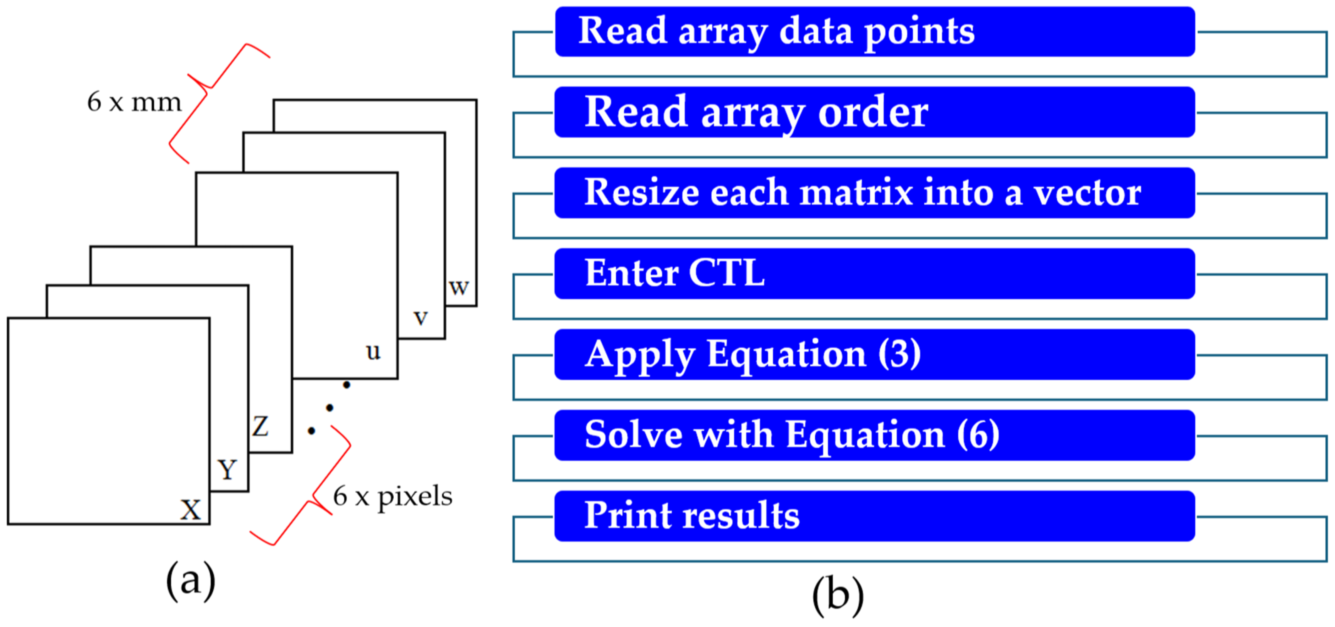
3. Proposed Scheme for Mode III Estimation

Following the same representation that Zhang and He [26] used, and that it was implemented somewhere else [29,38], Williams’ series for mode III can be rewritten as Equation (10).

$$w={\displaystyle \sum _{n=1}^N{c}_n}{p}_{n(r,\theta )}+T_z+R{z}_n$$

(10)

where Tz is rigid body displacement in perpendicular-to-plane and Rz_n rotation about perpendicular-to-crack-plane axis. An over-determined system, analog to Equation (5), can be used to solve Equation (10) for mode III as presented in Equation (11).

$$\left\{h_{III}\right\}=\left[b_{III}\right]\left\{{\Delta }_{III}\right\}$$

(11)

which can be expanded in Equation (12).

$$h_{III}=\left[\begin{array}{c}{w}_1\\ ⋮\\ w_M\\ \end{array}\right];{\Delta }_{III}=\left[\begin{array}{c}{C}_1\\ ⋮\\ C_M\\ \end{array}\right];b_{III}={\left[\begin{array}{c}{p}_{1(r_1,{\theta }_1)}\\ ⋮\\ p_{M(r_M,{\theta }_M)}\\ 1\\ 1\end{array}\right]}^T$$

(12)

where M is the number of data points, [h_III] is the concatenated vector of displacements, [Δ_III] the unknown coefficients in Williams’ series, and terms of function [b_III] are expressed in Equation (13).

$$p_{n(r,\theta )}={\displaystyle \frac{2r^{n-\raisebox{1ex}{$1$}\!\left/ \!\raisebox{-1ex}{$2$}\right.}}{G}}\left\{c_{n}Sin\left(n-{\displaystyle \frac{1}{2}}\right)\theta \right\}$$

(13)

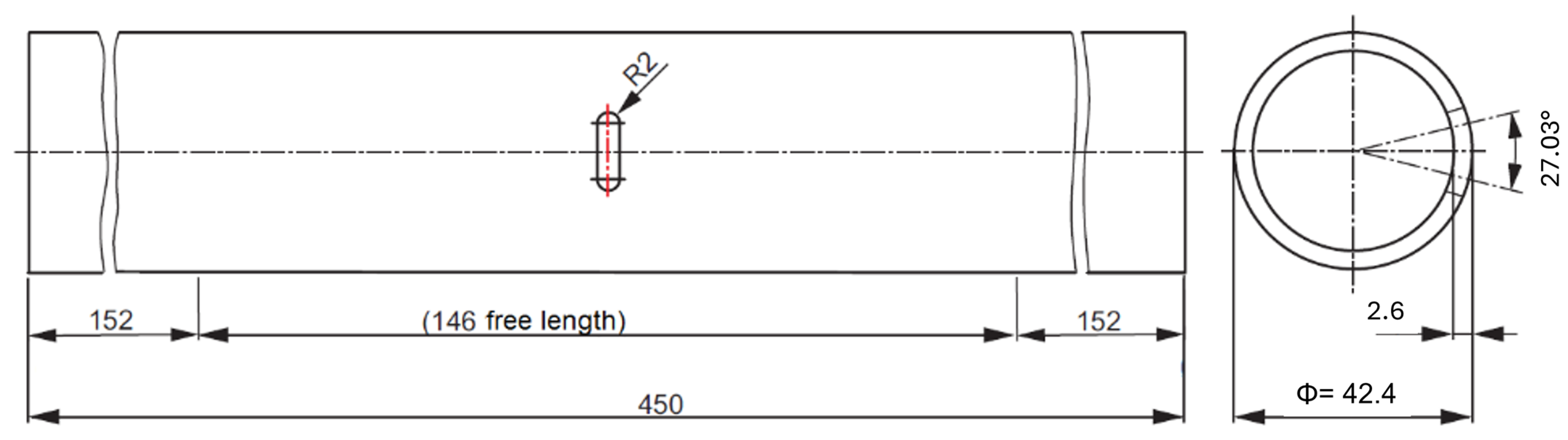
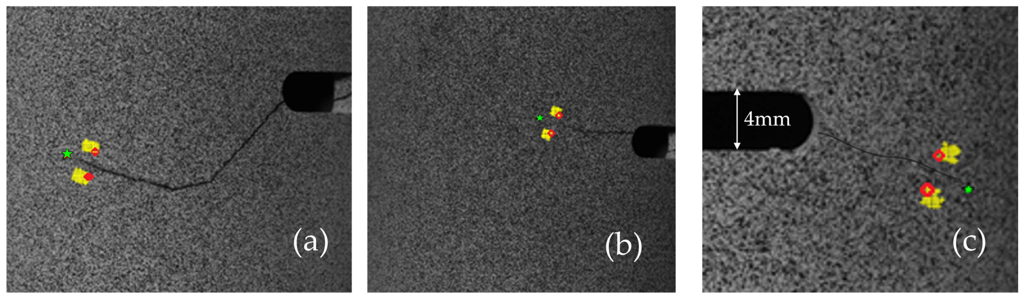
4. Materials and Methods

Figure 3 depicts a blueprint of one of the three S235 steel thin tubes (2.6 mm thickness) with a 42.4 mm outside diameter with a 14 mm long and 4 mm wide slit. The three tubes were loaded with sinusoidal in-phase tension and torsion (R-030), 90° out-of-phase tension and torsion (R-031), and 45° out-of-phase tension and torsion (R-033). In any case, the stress inversion ratio was −1, as shown in

Table 1. Applied loading settings and assessed SIF for every sample.

Specimen	R-030	R-031	R-033
Type of load	In-phase tension and torsion	90° out-of-phase tension and torsion	45° out-of-phase tension and torsion
Load ratio	RL = RT = −1	RL = RT = −1	RL = RT = −1
Measured SIF range	ΔKI, ΔKII, ΔKIII	ΔKI, ΔKII, ΔKIII	ΔKI, ΔKII, ΔKIII

. Specimens were photographed to be processed using 3D-VIC^® from Correlated Solutions (Columbia, SC, USA) with the DIC technique. The load was applied at 10 Hz frequency but lowered to 0.1 Hz for the DIC recording using two Allied Vision Tech. (Stadtroda, Germany) GT 2450 cameras with 2448 × 2050 resolution, giving a 3.45 μm × 3.45 μm pixel size. Finally, all tests used through–thickness cracks, with SIFs computed from recorded displacement fields. Extensive details concerning the testing experimental details (instruments, subset, correlation criteria, crack tip position, estimation, and more), as well as an explanation of the calculation methods for K, ΔK crack growth rate, and crack lengths, are described elsewhere [7,39]. Finally, a MATLAB^® 2021 (Natick, MA, USA) routine was written to test the method whose pseudocode is available in the web version.

The implemented algorithm takes data input as a MATLAB, *.mat, extension file. In that case, the data is an array (m × n × q) of coordinate matrices X, Y, Z, and displacement fields (both in mm), as well as displacements matrices u, v, w, and coordinate matrices x, y, z (both in pixels) as schematized in Figure 4a, whereas the steps are illustrated in Figure 4b.

Williams’ series has been used in curved samples with cracks smaller than the curvature. On the other hand, the LSM is a tool for solving over-determined systems. It finds the solution that minimizes the sum of the squared errors between the measured and the predicted responses.

Williams’ series for displacements were deducted for a planar surface, but the samples analyzed here were cylindrical. Therefore, if one assumes the distance between two points located in the same circumference of a cylinder as a straight line, there would be a mistake because of the specimen’s radius. Such inaccuracy is reduced by maintaining those two points close [10], which are CTL and displacement data. Hence, the AOI was determined by picking two 1 × 1 mm squares that were situated roughly 1 mm below the fracture tip because the compressive applied load produces negative stress forward of the crack tip, potentially producing negative K_I values. These AOIs were selected in order to exclude accumulated plasticity, which could result in nonlinear behavior and unrealistic SIF values both before and around the crack tip.

Furthermore, in an effort to reduce the accumulated plasticity ahead of the crack tip, displacement data was collected behind the crack tip, mimicking a COD clip gauge. That short distance minimizes the effects of accumulated plasticity, the uncertainty derived from the low correlation criteria given around the crack lips (which may provide unrealistic strains), and keeping the distance between AOI and CTL as short as possible to minimize the curvature effect as well as not getting into the near zone which would capture plastic strains. Furthermore, the fields must be aligned with the crack growth direction to comply with Williams’ premises. However, other factors like rugosity, trapped debris (which could enhance opening mode), and crack flank interlocking (which could impede sliding modes) are naturally taken into consideration. The COD model assumes that points A and B, from Figure 1, are ±180 degrees from the CTL [25], so Equation (1) is simplified to Equation (14).

$$\begin{array}{l}{K}_I=E{\displaystyle \frac{v_A-v_B}{4}}\sqrt{{\displaystyle \frac{2\pi }{r}}}\\ K_{II}=E{\displaystyle \frac{u_A-u_B}{4}}\sqrt{{\displaystyle \frac{2\pi }{r}}}\\ K_{III}=E{\displaystyle \frac{w_A-w_B}{4(1+\nu )}}\sqrt{{\displaystyle \frac{2\pi }{r}}}\end{array}$$

(14)

where E is the elastic modulus, and ν is the Poisson ratio.

Therefore, with the nonlinear effects restrictions in mind, Figure 5a shows the AOI for specimen R-031 (90° out-of-phase loading), Figure 5b for specimen R-033 (45° out-of-phase loading), and Figure 5c for specimen R-030 (in-phase loading) as yellow squares of about 1 × 1 mm. Moreover, the superimposed red dots represent the location where displacements were obtained for the COD model, Equation (14) whereas the green dots represent the crack tip. It is important to note that the displacement fields must be aligned according to the axis described in Williams’ model; this is the positive X axis coinciding with the crack growth direction. Furthermore, a COD clip gauge must be placed on the slit, and due to the nature of the crack growth, it may not give displacements that represent the stress field for the cases shown in Figure 5a,b.

5. Results and Discussion

The COD method would be the standard if one used a mouth-opening gauge placed at the crack end. So, SIFs in mode III are compared between the COD and the proposed LSM method. Furthermore, SIFs in modes I and II were also computed for the three loading cases using the LSM formulation, as described in Equations (3)–(6), so the chosen AOI is validated.

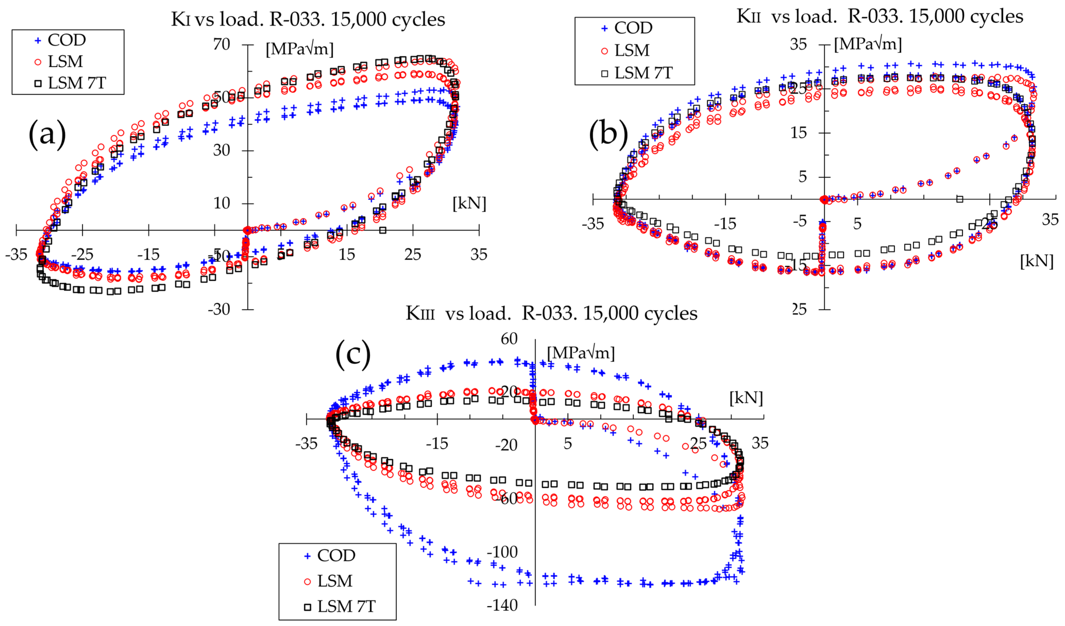
5.1. Results for Non-Proportional (45° Out-of-Phase Tension and Torsion) Loading

Figure 6a–c compares SIF obtained with the proposed method to the COD method (relative displacements of two opposite-to-crack points, Equation (14)) for modes I, II, and III, respectively, for R-031 after 33,000 loading cycles. The loading in this sample is non-proportional, with a 90° out-of-phase angle between axial and torque loads. For the three modes, it is seen that both methods agree in the proportional part (ramping-up and ramping-down loads). For mode I, both methods show identical results for the non-proportional loading part. For mode II, the LSM shows larger values for the COD method, whereas for mode III, the LSM method shows slightly lower values for the LSM method. In all cases, the maximum values in both methods exhibit maximum values at maximum axial load. Perhaps this is due to the maximum crack opening, which eliminates nonlinear effects such as rugosity, crack flank interlocking, and trapped debris that might hinder the development of sliding modes. Figure 6a shows the strong nonlinearity between mode I loading and unloading paths. One differential aspect of the load is the full load inversion for axial force and torque. So, one might need to crosscheck the results with the load to avoid incorrectly interpreting it as a negative K_I value instead of a ΔK_I.

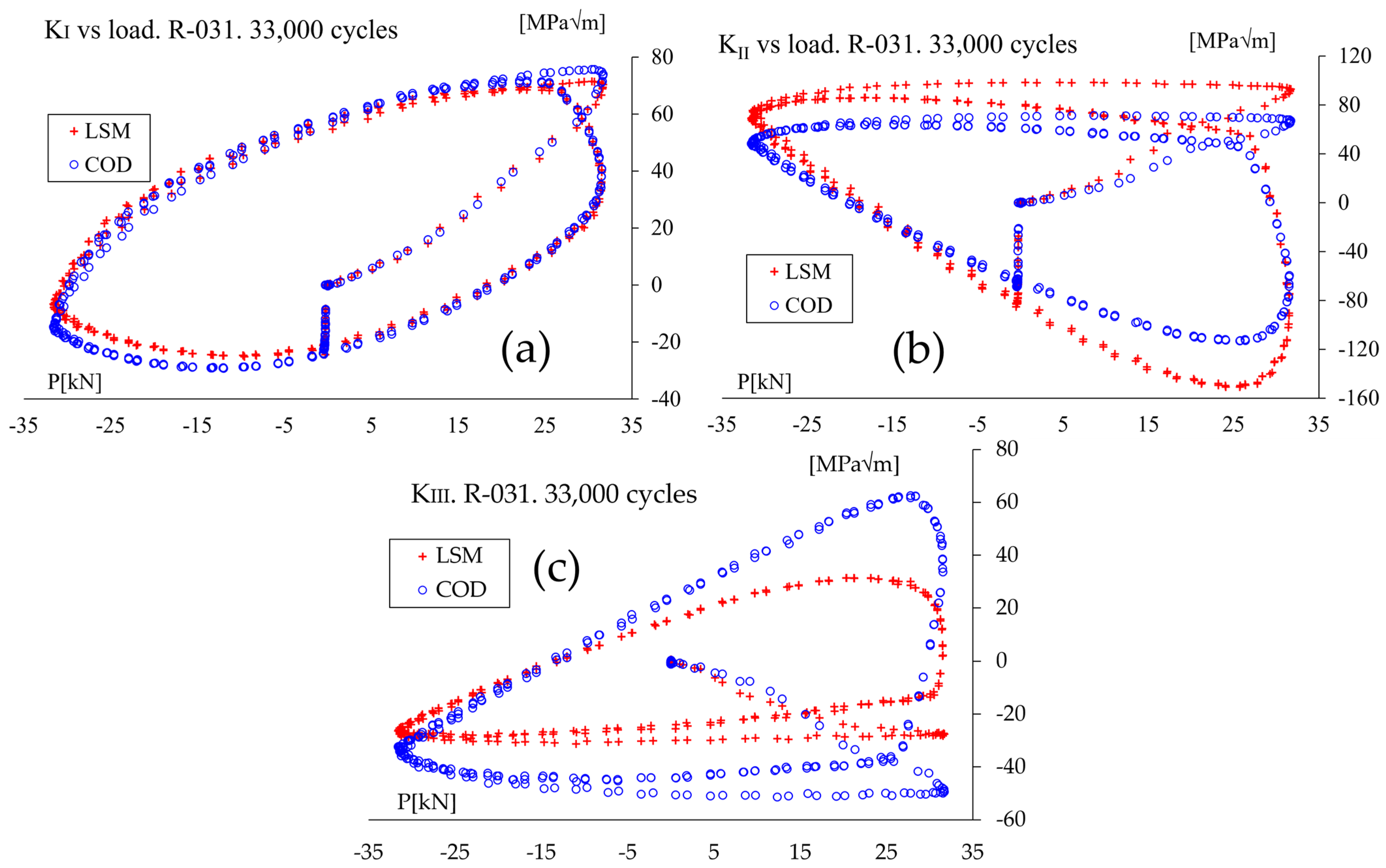
5.2. Results for Non-Proportional (90° Out-of-Phase Tension and Torsion) Loading

Figure 7a–c compares SIF obtained with the proposed method to the COD method (relative displacements of two opposite-to-crack points, Equation (14)) for modes I, II, and III, respectively, for the R-033 sample after 15,000 loading cycles. The LSM method was applied for this sample using one and seven terms of Williams’ series. Camacho et al. [40] used 2, 3, and 4 terms, finding slight differences for mode I, and Harilal et al. [38] used up to 10 terms, finding that K_I stabilized after using as little as two terms. Strohmann et al. [29] discussed how the number of terms can influence fracture mechanics parameters and FCG stability, but there is limited understanding of their physical meaning. Recently, Kolditz et al. [41] used a similar approach, but used the stability of the energy release rate in a phase–field simulation as a benchmark. On the other hand, Ramesh et al. [27] found that after nine terms, the differences in the results are negligible in photoelastic image analysis. So, to perform an analysis, one typically starts with one term in the Williams’ series and gradually raises the number until SIF results stabilize. The attached algorithm includes the number of terms as a variable in the Supplemental Material.

On the other hand, SIFs do not show proportional behavior to either axial or torsional loads for most of the loading range. Such nonlinearity can indicate that crack blunting is present as the crack lips are displaced when the load is reduced. Additionally, one can see how sliding modes II and III stay about constant after the maximum axial load is reached. After the crack opens, hence disabling fatigue crack closure, the crack edges are free to slide, and the torque load keeps them open. However, K_II and K_III seem to reach zero at the smaller axial load. This may be attributed to rugosity and crack flank locking (attributed to the crack’s curvature) interfering with in-plane sliding and being unable to overcome the friction. Finally, when comparing Figure 7a–c, one can see how, at maximum axial load, sliding modes are the largest but in opposite directions. As the axial load ramps down, K_III sharply falls, and when the axial load goes up, K_II rises. One must remember that under the applied fatigue loading, such continuous sliding would eventually produce crack smoothing [9], thus enhancing mode III.

5.3. Results for Proportional (In-Phase Tension and Torsion) Loading

SIF obtained using the proposed LSM approach and the COD method (relative displacements of two opposite-to-crack points, Equation (14)) for modes I, II, and III, respectively, for the R-030 sample after 13,000 loading cycles are compared in Figure 8a–c. One can see that the loading and unloading phases take independent paths, which is identified as a consequence of imposed plasticity. Figure 8a illustrates how K_I increases for positive loads, but the approaches differ slightly in their negative slopes. The negative part of K_I is a mixture of elastic compression and plasticity reversion created by the negative part of the axial load, which results in positive residual stresses upon unloading [9]. This could be explained by the fact that some of the positive plastic strains created when the crack was fully open are now reversed [9]. Nonetheless, when the crack is closed, the singularity required by the Westergaard stress function does not occur.

Summarizing SIFs’ evolution during a cycle obtained from displacements, one can say that for proportional loading in-phase tension–torsion, the SIFs’ ratio remains quasi-constant other than what is attributed to accumulated plasticity, rugosity, crack flanks interlocking, and perhaps trapped debris. On the other hand, for the non-proportional load samples (90° out-of-phase and 45° out-of-phase tension and torsion), the SIFs change at different ratios. In these two cases, such extra difference is attributed to the constant change of applied loading.

5.4. Discussion

It has been argued [4,6,7,16,42,43] that leaving K_III out of K_eq may lead to an imprecise crack path and crack initiation [12]. However, when using full-field measurement non-linearities, such as fatigue-induced plasticity, crack flank interlocking, rugosity, and trapped debris are already accounted for [7,31]. In these cases, including full-field measurements allows the capture of such a degree of plasticity. This means these SIFs could not be calculated from numerical simulations [44]. The proposed method captures the full extent of SIF and SIF ranges. So, in that sense, SIFs are deemed as effective.

However, negative K_I values do not make physical sense. For negative relative displacements to occur, the crack lips would need to penetrate each other, which is physically impossible. Figure 6a and Figure 7a show a strong nonlinearity between the loading and unloading paths in mode I. One differential aspect of the applied axial load is the full inversion. So, one might need to pay close attention so as not to incorrectly interpret it as a negative K_I value instead of a SIF range. So, the growing negative K_I values shown in sample R-030 under negative load show a limitation of the proposed method and can be interpreted as crack lips touching each other. However, for sliding modes II and III, the negative sign indicates the relative displacements change directions. According to Equation (9), such direction provides the direction of the crack kinking angle [25]. It is also observed that sliding modes develop in opposite directions, confirmed by the two methods. This may be attributed to one sliding mode that can dissipate energy faster than the other one, most likely credited to rugosity [44].

Moreover, Sapora et al. [11] recently acknowledged the interaction and possible overlapping between mode III and other modes. Similarly, a rise in K_II implied a reduction of K_I and vice versa, and Miao et al. [6] found a coupling effect between modes I and III, and recently Moradi et al. [23] confirmed such coupling for I and II, II, and III, and I and III at least for a composite material. With that in mind, Figure 9 represents a crack with three opening modes where the displacement vector over the surface is plotted as δ, the displacements in each direction are plotted as δ_i, and α and Ψ are the in-plane and out-of-plane crack kinking angles, respectively. If the value of total displacement δ stays constant but changes direction, the ratio of modes II and III will change. Furthermore, Equation (14) shows the relation between displacement and SIF; hence, a change in displacement creates a shift in SIF. Although such behavior may not impact the fatigue crack growth rate if Keq stays the same, it undoubtedly will impact SIFs’ values and the crack propagation, as recently discussed by Gómez et al. [31]. If K_II rises, it favors α growth (in-plane direction), whereas if K_III goes up, Ψ growth is favored (out-of-plane direction). Moreover, microscopic crack growth was not studied. This paper shows a method to calculate the K_III, so FCG is fully accounted for and not underestimated at the macro level. This is important as Pook [16] observed that mild steel exhibiting mode III displacements tends to branch to mode I cracks that most likely would produce faster FCG. Nonetheless, CP prediction for 3D cracks is a challenging task [12]. This paper proposes a method to calculate mode SIF III to be included in such estimation.

On the other hand, the proposed method and others used to calculate SIFs, such as the COD, the decomposition integral [13], or circular J integral [36], heavily rely on the crack tip position; for a numerical approach, this is not a problem as the crack tip location is known beforehand, but for an experimental work, it is an unknown variable. However, such an evaluation is out of the scope of this paper and will be addressed elsewhere. Furthermore, using LEFM requires that its intrinsic assumptions (sharp crack tip, linear boundary conditions, homogeneous and linear elastic material, and small-scale yielding) are met. Stresses and deformations must be sufficiently linear to comply with the linear elastic assumption of the Westergaard stress function. Furthermore, when selecting the AOI, one must check the stress field and the plastic zone to discard the displacements in the near region. One must remember such limitations when selecting a method to calculate SIFs from experimental fields.

6. Conclusions

A method to establish K_III using full-field displacement data, obtained with the Digital Image Correlation technique, was proposed and implemented. However, the method could be used with displacement fields obtained in any manner. SIF calculation is more robust when using more than two data points. The procedure was applied to three thin tubes subjected to axial and torsional loads: one in-phase and two out-of-phase. The comparison of results with the COD method shows an agreement for one case of proportional and two cases of non-proportional loads. The pseudocode reflecting the proposed method is available on the web version of the article. The proposed method captures the accumulated plasticity, providing less noisy results. Finally, the SIF evolution during proportional and non-proportional loading was described, showing a pronounced nonlinearity attributed to the constant change of applied loading for the latter case.

The proposed method data fits displacements to Williams’ solution for mode III, which is an infinite plate. When approximating the distance from the crack tip to the measured points, the curvature error induced by the camera measurements introduced an error using a straight line instead of the perimeter. However, in this manuscript, the distance between the crack tip and the measured area was kept as close as 1 mm, so the error was minimized, always ensuring that only elastic strains were used to compute SIF. An approach to solve this could use the proposed approximations for K_I based on curvature as described in [8,40], which could provide more accurate results. However, there are no solutions for sliding modes that allow further improvement. Finally, optimizing the area of interest (AOI) selection could mitigate the impact of accumulated plasticity and enhance the accuracy of SIF calculations.

Although not tested in this paper, the method could be implemented with displacement fields from any source, such as other experimental techniques, or from numerical simulations. The latter case has advantages as the crack tip location is known in advance, thus reducing the uncertainty in SIF calculation. Furthermore, numerical simulations deliver through-the-thickness displacements, so the maximum SIF could be calculated instead of only surface displacements as presented and tested here.

References

1. Kotousov, A.; Lazzarin, P.; Berto, F.; Pook, L.P. Three-Dimensional Stress States at Crack Tip Induced by Shear and Anti-Plane Loading. Eng. Fract. Mech. 2013, 108, 65–74. [Google Scholar] [CrossRef]
2. Fremy, F.; Pommier, S.; Poncelet, M.; Raka, B.; Galenne, E.; Courtin, S.; Roux, J.C. Le Load Path Effect on Fatigue Crack Propagation in I + II + III Mixed Mode Conditions—Part 1: Experimental Investigations. Int. J. Fatigue 2014, 62, 104–112. [Google Scholar] [CrossRef]
3. Schöllmann, M.; Richard, H.A.; Kullmer, G.; Fulland, M. A New Criterion for the Prediction of Crack Development in Multiaxially Loaded Structures. Int. J. Fract. 2002, 117, 129–141. [Google Scholar] [CrossRef]
4. Bonniot, T.; Doquet, V.; Mai, S.H. Mixed Mode II and III Fatigue Crack Growth in a Rail Steel. Int. J. Fatigue 2018, 115, 42–52. [Google Scholar] [CrossRef]
5. Ju, Y.; Zhang, Y.; Wang, K.; Zhou, H. 3D-Generalized Maximum Tangential Strain Criterion for Predicting Mixed-Mode I/II/III Fracture Initiation of Brittle Materials Considering T-Stress Effects. Theor. Appl. Fract. Mech. 2024, 131, 104382. [Google Scholar] [CrossRef]
6. Miao, X.; Zhang, J.; Hong, H.; Peng, J.; Zhou, B.; Li, Q. Study on Elastic Mixed Mode Fracture Behavior and II-III Coupling Effect. Materials 2023, 16, 4879. [Google Scholar] [CrossRef] [PubMed]
7. Vormwald, M.; Hos, Y.; Freire, J.L.F.; Gonzáles, G.L.G.; Díaz, J.G. Crack Tip Displacement Fields Measured by Digital Image Correlation for Evaluating Variable Mode-Mixity during Fatigue Crack Growth. Int. J. Fatigue 2018, 115, 53–66. [Google Scholar] [CrossRef]
8. Sipos, A.A.; Cao, S. About Measuring the Stress Intensity Factor of Cracks in Curved, Brittle Shells. Frat. Ed. Integrità Strutt. 2024, 18, 1–17. [Google Scholar] [CrossRef]
9. Petureau, L.; Doquet, V.; Dieu, B. Influence of a Static Torque on Plasticity and Asperity-Induced Closure Effects during Fatigue Crack Growth in Bainitic Steel Cylinders Loaded in Push-Pull. Int. J. Fatigue 2022, 155, 106628. [Google Scholar] [CrossRef]
10. Diaz, J.G.; Marques, L.F.N.; Guzmán, R.E. Mixed-Mode Stress Intensity Factors for Tubes under Pure Torsion Loading. Key Eng. Mater. 2018, 774, 373–378. [Google Scholar] [CrossRef]
11. Mirzaei, A.M.; Sapora, A.; Cornetti, P. Asymptotic Stress Field for the Blunt and Sharp Notches in Bi-Material Media Under Mode III Loading. J. Appl. Mech. 2024, 91, 051008. [Google Scholar] [CrossRef]
12. Ju, Y.; Zhang, Y.; Yu, H. Numerical Prediction and Experiments for 3D Crack Propagation in Brittle Materials Based on 3D-Generalized Maximum Tangential Strain Criterion. Theor. Appl. Fract. Mech. 2025, 135, 104747. [Google Scholar] [CrossRef]
13. Molteno, M.R.; Becker, T.H. Mode I–III Decomposition of the J-Integral from DIC Displacement Data. Strain 2015, 51, 492–503. [Google Scholar] [CrossRef]
14. Yu, X.; Li, L.; Proust, G. Fatigue Crack Growth of Aluminium Alloy 7075-T651 under Proportional and Non-Proportional Mixed Mode I and II Loads. Eng. Fract. Mech. 2017, 174, 155–167. [Google Scholar] [CrossRef]
15. Wang, Y.; Wang, W.; Zhang, B.; Li, C.-Q. A Review on Mixed Mode Fracture of Metals. Eng. Fract. Mech. 2020, 235, 107126. [Google Scholar] [CrossRef]
16. Pook, L. The Fatigue Crack Direction and Threshold Behaviour of Mild Steel under Mixed Mode I and III Loading. Int. J. Fatigue 1985, 7, 21–30. [Google Scholar] [CrossRef]
17. Saboori, B.; Ayatollahi, M.R. A Novel Test Configuration Designed for Investigating Mixed Mode II/III Fracture. Eng. Fract. Mech. 2018, 197, 248–258. [Google Scholar] [CrossRef]
18. Aliha, M.R.M.; Bahmani, A.; Akhondi, S. Determination of Mode III Fracture Toughness for Different Materials Using a New Designed Test Configuration. Mater. Des. 2015, 86, 863–871. [Google Scholar] [CrossRef]
19. Jalayer, R.; Saboori, B.; Ayatollahi, M.R. A Novel Test Specimen for Mixed Mode I/II/III Fracture Study in Brittle Materials. Fatigue Fract. Eng. Mater. Struct. 2023, 46, 1908–1920. [Google Scholar] [CrossRef]
20. Pham, K.H.; Ravi-Chandar, K. On the Growth of Cracks under Mixed-Mode I + III Loading. Int. J. Fract. 2016, 199, 105–134. [Google Scholar] [CrossRef]
21. Bahrami, B.; Nejati, M.; Ayatollahi, M.R.; Driesner, T. True Mode II Fracturing of Rocks: An Axially Double-Edge Notched Brazilian Disk Test. Rock. Mech. Rock. Eng. 2022, 55, 3353–3365. [Google Scholar] [CrossRef]
22. Qin, X.; Su, H.; Yu, L.; Wang, H.; Jiang, Y.; Pham, T.N. Differential Response of Fracture Characterization of Mode III Fracture in Sandstone Under Dynamic Versus Static Loading. Fatigue Fract. Eng. Mater. Struct. 2024, 48, 1315–1329. [Google Scholar] [CrossRef]
23. Moradi, E.; Zeinedini, A. On the Mixed Mode I/II/III Inter-Laminar Fracture Toughness of Cotton/Epoxy Laminated Composites. Theor. Appl. Fract. Mech. 2020, 105, 102400. [Google Scholar] [CrossRef]
24. Zhao, Y.; Zheng, K.; Wang, C. Review of Fracture Test Methods. In Rock Fracture Mechanics and Fracture Criteria; Springer: Singapore, 2024; pp. 29–45. [Google Scholar]
25. Maneschy, J.E.; Miranda, C.A.d.J. Application of Fracture Mechanics in the Nuclear Industry, 1st ed.; Eletrobras, Ed.; Eletrobras: Rio de Janeiro, Brazil, 2023; ISBN 9788599092026. [Google Scholar]
26. Zhang, R.; He, L. Measurement of Mixed-Mode Stress Intensity Factors Using Digital Image Correlation Method. Opt. Lasers Eng. 2012, 50, 1001–1007. [Google Scholar] [CrossRef]
27. Ramaswamy, G.; Ramesh, K.; Saravanan, U. Influence of Contact Stresses on Crack-Tip Stress Field: A Multiparameter Approach Using Digital Photoelasticity. Exp. Mech. 2024, 64, 785–804. [Google Scholar] [CrossRef]
28. Ju, S.H.; Chung, H.Y. Accuracy and Limit of a Least-Squares Method to Calculate 3D Notch SIFs. Int. J. Fract. 2007, 148, 169–183. [Google Scholar] [CrossRef]
29. Strohmann, T.; Melching, D.; Paysan, F.; Dietrich, E.; Requena, G.; Breitbarth, E. Next Generation Fatigue Crack Growth Experiments of Aerospace Materials. Sci. Rep. 2024, 14, 14075. [Google Scholar] [CrossRef] [PubMed]
30. Gonzalez, M.; Teixeira, P.; Wrobel, L.C.; Martinez, M. A New Displacement-Based Approach to Calculate Stress Intensity Factors with the Boundary Element Method. Lat. Am. J. Solids Struct. 2015, 12, 1677–1697. [Google Scholar] [CrossRef]
31. Gómez-Gamboa, E.; Díaz-Rodríguez, J.G.; Mantilla-Villalobos, J.A.; Bohórquez-Becerra, O.R.; Martínez, M.d.J. Experimental and Numerical Evaluation of Equivalent Stress Intensity Factor Models under Mixed-Mode (I+II) Loading. Infrastructures 2024, 9, 45. [Google Scholar] [CrossRef]
32. Díaz, J.G.; Freire, J.L.d.F. LEFM Crack Path Models Evaluation under Proportional and Non-Proportional Load in Low Carbon Steels Using Digital Image Correlation Data. Int. J. Fatigue 2022, 156, 106687. [Google Scholar] [CrossRef]
33. Langlois, C.R.; Gravouil, A.; Baietto, M.-C.; Réthoré, J. Three-dimensional Simulation of Crack with Curved Front with Direct Estimation of Stress Intensity Factors. Int. J. Numer. Methods Eng. 2015, 101, 635–652. [Google Scholar] [CrossRef]
34. Kujawski, D. Discussion and Comments on KOP and ∆Keff. Materials 2020, 13, 4959. [Google Scholar] [CrossRef] [PubMed]
35. Tavares, S.M.O.; de Castro, P.M.S.T. Equivalent Stress Intensity Factor: The Consequences of the Lack of a Unique Definition. Appl. Sci. 2023, 13, 4820. [Google Scholar] [CrossRef]
36. Yoneyama, S.; Arikawa, S.; Kusayanagi, S.; Hazumi, K. Evaluating J-Integral from Displacement Fields Measured by Digital Image Correlation. Strain 2014, 50, 147–160. [Google Scholar] [CrossRef]
37. Richard, H.A.; Fulland, M.; Sander, M. Theoretical Crack Path Prediction. Fatigue Fract. Eng. Mater. Struct. 2004, 28, 3–12. [Google Scholar] [CrossRef]
38. Harilal, R.; Vyasarayani, C.P.; Ramji, M. A Linear Least Squares Approach for Evaluation of Crack Tip Stress Field Parameters Using DIC. Opt. Lasers Eng. 2015, 75, 95–102. [Google Scholar] [CrossRef]
39. Vormwald, M.; Hos, Y.; Freire, J.L.F.; Gonzáles, G.L.G.; Díaz, J.G. Variable Mode-Mixity during Fatigue Cycles—Crack Tip Parameters Determined from Displacement Fields Measured by Digital Image Correlation. Frat. Ed. Integrità Strutt. 2017, 11, 314–322. [Google Scholar] [CrossRef]
40. Camacho-Reyes, A.; Gómez-Gonzales, G.; Vasco-Olmo, J.; Díaz, F.A. Cálculo de Los Parámetros Gobernantes de La Singularidad En El Vértice de Grieta En Superficies Cilíndricas Empleando Geometría Diferencial y Correlación Digital de Imágenes 3D. Rev. Mecánica La. Fract. 2023, 5, 63–67. [Google Scholar]
41. Kolditz, L.M.; Dray, S.; Kosin, V.; Fau, A.; Hild, F.; Wick, T. Employing Williams’ Series for the Identification of Fracture Mechanics Parameters from Phase-Field Simulations. Eng. Fract. Mech. 2024, 307, 110298. [Google Scholar] [CrossRef]
42. Tschegg, E.K. Sliding Mode Crack Closure and Mode III Fatigue Crack Growth in Mild Steel. Acta Metall. 1983, 31, 1323–1330. [Google Scholar] [CrossRef]
43. Ritchie, R.; McClintock, F.; Tschegg, E.; Nayeb-Hashemi, H. Mode III Fatigue Crack Growth Under Combined Torsional and Axial Loading. In Multiaxial Fatigue; ASTM: West Conshohocken, PA, USA, 1985; pp. 203–227. [Google Scholar]
44. Kujawski, D.; Vasudevan, A.K.; Ricker, R.E.; Sadananda, K. On 50 Years of Fatigue Crack Closure Dispute. Fatigue Fract. Eng. Mater. Struct. 2023, 46, 2816–2829. [Google Scholar] [CrossRef]
Figure 1. Notation for the coordinate system and displacements around a cracked domain showing parallel-to-crack u-displacement, perpendicular-to-crack v-displacement, and out-of-plane w-displacement.
Applsci 15 03404 g001
Figure 2. Effect of KIII on (a) Tanaka’s Keq with Poisson ratio = 0.3 (b) crack kinking angle, according to Richard.
Applsci 15 03404 g002
Figure 3. Thin tubes, dimensions in mm. From [7].
Applsci 15 03404 g003
Figure 4. Schematics for data used (a) input format needed, and (b) steps used in the implementation.
Applsci 15 03404 g004
Figure 5. Data source for (a) R-031 specimen, (b) R-033 specimen, (c) R-030 specimen.
Applsci 15 03404 g005
Figure 6. R-031 (45° out-of-phase tension and torsion) results comparison between COD and LSM methods: (a) KI, (b) KII, (c) KIII.
Applsci 15 03404 g006
Figure 7. R-033 (90° out-of-phase tension and torsion results in comparison between COD and LSM methods using one and seven terms methods: (a) KI, (b) KII, (c) KIII.
Applsci 15 03404 g007
Figure 8. R-030 (in-phase tension–torsion) results comparison between COD and LSM methods: (a) KI, (b) KII, (c) KIII.
Applsci 15 03404 g008
Figure 9. Sliding displacements over the crack’s fracture plane. Adapted from [6].
Applsci 15 03404 g009