Research on a Lightweight Rail Surface Condition Identification Method for Wheel–Rail Maximum Adhesion Coefficient Estimation

Abstract

The rail surface condition is a critical factor influencing wheel–rail adhesion performance. To address the engineering challenges associated with existing rail surface condition identification models, such as high-parameter complexity, significant computational delay, and the difficulty of onboard deployment, a lightweight rail surface condition identification method integrating knowledge distillation and transfer learning is proposed. A rail surface image dataset is constructed, covering typical working conditions, including dry, wet, and oily surfaces. A “teacher-student” collaborative optimization framework is developed, in which GoogLeNet, fine tuned via transfer learning, serves as the teacher network to guide the MobileNet student network, which is also fine tuned through transfer learning, thereby achieving model compression. Additionally, an FP16/FP32 mixed-precision computing strategy is employed to accelerate the training process. The experimental results demonstrate that the optimized student model has a compact size of only 4.21 MB, achieves an accuracy of 97.38% on the test set, and attains an inference time of 0.0371 s. Integrating this model into the estimation system of the maximum adhesion coefficient for heavy-haul locomotives enhances estimation confidence, reduces estimation errors under varying operating conditions, and provides real-time and reliable environmental perception for optimizing adhesion control strategies. This approach holds significant engineering value in improving adhesion utilization under complex wheel–rail contact conditions.

1. Introduction

The wheel–rail adhesion state is a critical factor determining the traction and braking performance of heavy-haul trains. The dynamic variations in the adhesion coefficient, primarily influenced by third-body media (e.g., water, oil) on the rail surface, directly impact operational safety and control precision [1,2,3,4,5]. Therefore, accurately identifying the rail surface condition and transmitting this information to the train in real time is essential for enabling timely control system responses and ensuring high-performance train operation. The region near the maximum adhesion coefficient represents the optimal utilization of traction power, making it a focal point in adhesion control research.

Current methods for estimating the maximum adhesion coefficient exhibit significant limitations. The adhesion slope method [6,7,8] is constrained by a narrow range of model observation frequency points, while the creep–slip velocity method [9] faces challenges in accurately obtaining the creep–slip velocity, limiting its practical applications. Although fuzzy control mitigates model dependency, its reliance on one-dimensional dynamic inputs (e.g., creep–slip velocity, adhesion coefficient) results in insufficient confidence and accuracy in complex operating conditions [10]. Integrating multi-source sensing information, particularly real-time visual identification of the rail surface condition, can enhance both the accuracy and reliability of maximum adhesion coefficient estimation while improving environmental adaptability.

In recent years, deep learning-based visual identification of rail surface conditions has achieved promising results. While high-precision classification models, such as ResNet and VGG, have demonstrated strong performance, their high computational complexity (e.g., ResNet-18 contains 11.7M parameters) limits their applicability to real-time, embedded in-vehicle platforms [11]. Lightweight models [12,13,14] and model compression techniques [15,16,17,18] can reduce computational overhead but often suffer from accuracy degradation when trained on small datasets. Therefore, achieving high accuracy, low latency, and strong generalizability in rail surface condition identification remains a critical challenge.

Through the aforementioned analysis, this study aims to address the engineering challenges faced by existing rail surface state identification models in terms of accuracy, computational complexity, and feasibility for onboard deployment. Simultaneously, it seeks to enhance the confidence and accuracy of maximum adhesion coefficient estimation by incorporating rail surface state information. The key contributions of this study are as follows:

(1)

A lightweight rail surface condition identification method is proposed to achieve a balance between model accuracy and real-time performance. Specifically, a multi-condition rail surface state image dataset is constructed, and a “teacher-student” co-optimization framework is established. By leveraging knowledge distillation, the multi-scale feature extraction capability of the teacher model is effectively transferred to the student model, thereby maintaining high recognition accuracy under lightweight constraints. Furthermore, a mixed-precision training framework is embedded to enhance computational efficiency, thereby meeting the real-time requirements of the onboard system.

(2)

A multi-source information fusion mechanism is designed to integrate rail surface condition information into the maximum adhesion coefficient estimation system. This study adopts a fuzzy control-based approach to achieve multi-source information fusion, where the application of fuzzy logic significantly mitigates the impact of information uncertainty on adhesion coefficient estimation. Consequently, the accuracy of maximum adhesion coefficient estimation in complex environments is effectively improved.

The proposed approach satisfies the requirements of high accuracy, low latency, and strong generalization in rail surface condition identification (test set accuracy ≥ 90%, model inference time ≤ 0.04 s, and the number of parameters ≤ 5 M). Additionally, it provides a more accurate threshold for the maximum adhesion coefficient, thereby facilitating optimal adhesion control.

The rest of this paper is organized as follows. Section 2 describes the overall framework of the method, including the multi-source data input module, lightweight rail surface condition identification module, and fuzzy fusion estimation module. Section 3 shows the experimental results of the corresponding modules and analyzes them. Section 4 summarizes the research results and discusses the future research direction.

2. General Structure of the Methodology

The overall architecture of the proposed lightweight rail surface condition identification method for maximum adhesion coefficient estimation is illustrated in Figure 1. This method comprises three core modules: (A) a multi-source data input module, (B) a lightweight rail surface condition identification module, and (C) a fuzzy fusion estimation module.

Module A is responsible for acquiring and pre-processing rail surface condition images using industrial cameras while simultaneously obtaining real-time train operation data, including creep and slide speed and adhesion coefficients, based on the HXD1 locomotive’s traction dynamics model. Module B processes the rail surface images acquired by Module A and employs a teacher–student collaborative optimization framework. Specifically, GoogLeNet and MobileNet serve as the backbone networks, where transfer learning is utilized to fine tune the high-level feature pyramid, enabling multi-scale feature extraction. Furthermore, knowledge distillation enhances the performance of the student model, while a mixed-precision training strategy improves computational efficiency. Ultimately, this module achieves real-time and accurate rail surface condition identification. Module C implements a multi-source information fusion mechanism that integrates train operation data from Module A. By designing membership functions and fuzzy logic rules, the system estimates the maximum adhesion coefficient and further refines the estimation using the rail surface condition information derived from Module B. The final estimated adhesion coefficient is then compared against the ideal value for evaluation and validation.

The key innovations of this approach are as follows. The first is a knowledge distillation-driven lightweight identification model, which enhances both real-time performance and deployability. The second is a fuzzy logic-based multi-source information fusion strategy, improving the estimation accuracy and confidence of the maximum adhesion coefficient. The third is a dual-modal “vision-dynamics” data processing mechanism, enhancing the system’s adaptability and robustness under complex operational conditions.

2.1. Multi-Source Data Input Module

This module facilitates “vision-dynamics” bimodal data acquisition, integrating real-time data collection and processing through an industrial camera and the constructed train traction dynamics model. It provides the necessary inputs for subsequent rail surface condition identification and maximum adhesion coefficient estimation.

Visual modality. To capture image data of the rail surface conditions, a dedicated data acquisition platform is developed, employing industrial cameras to capture rail surface images under dynamic conditions. These images encompass three typical operational states: dry, wet, and oily. The image data undergo a series of pre-processing steps, including grayscaling, denoising, enhancement, perspective transformation, rail surface area extraction, and data augmentation. These procedures aim to enhance micro-textural features, augment the training dataset, and fulfill the input requirements for the subsequent neural network model.

Dynamic modes. Drawing on the traction dynamics model of the HXD1 locomotive, this modality emphasizes the mathematical representation of the wheel–rail interaction and adhesion force, with particular attention to the influence of creep–slip velocity on the adhesion force. A full-dimensional state observer is incorporated to estimate the real-time adhesion coefficient between the wheels and rails, integrating the kinetic model to reflect the adhesion state. The real-time creep–slip velocity and the estimated adhesion coefficient serve as crucial data inputs for the subsequent estimation of the maximum adhesion coefficient.

2.2. Lightweight Rail Surface Condition Identification Module Based on Knowledge Distillation and Transfer Learning

Based on the preceding analysis, it is evident that rail surface condition identification must simultaneously address the demands of high accuracy, low latency, and strong generalization. To enhance model inference speed while maintaining high identification accuracy, this study proposes a lightweight identification approach that leverages knowledge distillation and transfer learning techniques, as illustrated in Figure 2. GoogLeNet is selected as the teacher model due to the well-established advantages of its Inception module in multi-scale feature extraction [19]. Compared with ResNet, which is widely adopted in existing studies on rail surface state recognition, GoogLeNet significantly reduces the number of parameters while having a deeper network structure. This allows it to achieve a better balance between computational efficiency and accuracy, making it well suited for the task of this study. MobileNet is chosen as the student model due to its depthwise separable convolution structure, which demonstrates superior performance in resource-constrained environments [13]. Compared with other classical lightweight models, such as EfficientNet and ShuffleNet, MobileNet offers a moderate number of parameters and a shallower network depth, thereby achieving a better trade-off between accuracy and inference speed. Through knowledge distillation, the teacher model’s knowledge is efficiently transferred to the student model, thereby improving inference efficiency without compromising accuracy. Furthermore, to further enhance the model’s generalization capability, transfer learning is employed, utilizing pre-trained ImageNet weights for the rail surface condition identification task, which also significantly reduces model training time. During the training phase, a mixed-precision training strategy is incorporated to optimize computational efficiency. By combining these techniques, a lightweight rail surface condition identification model is developed, achieving both high efficiency and reliability.

2.2.1. Feature Optimization Based on Transfer Learning

In this study, model-based transfer learning [20] is employed to accelerate model convergence and enhance both model accuracy and generalization. In the task of rail surface condition identification, the primary advantage of transfer learning lies in its ability to improve task-specific feature learning by transferring the feature representations learned by the teacher model (GoogLeNet) and the student model (MobileNet) from a large-scale image dataset. This process ultimately enhances the model’s identification accuracy and generalization performance.

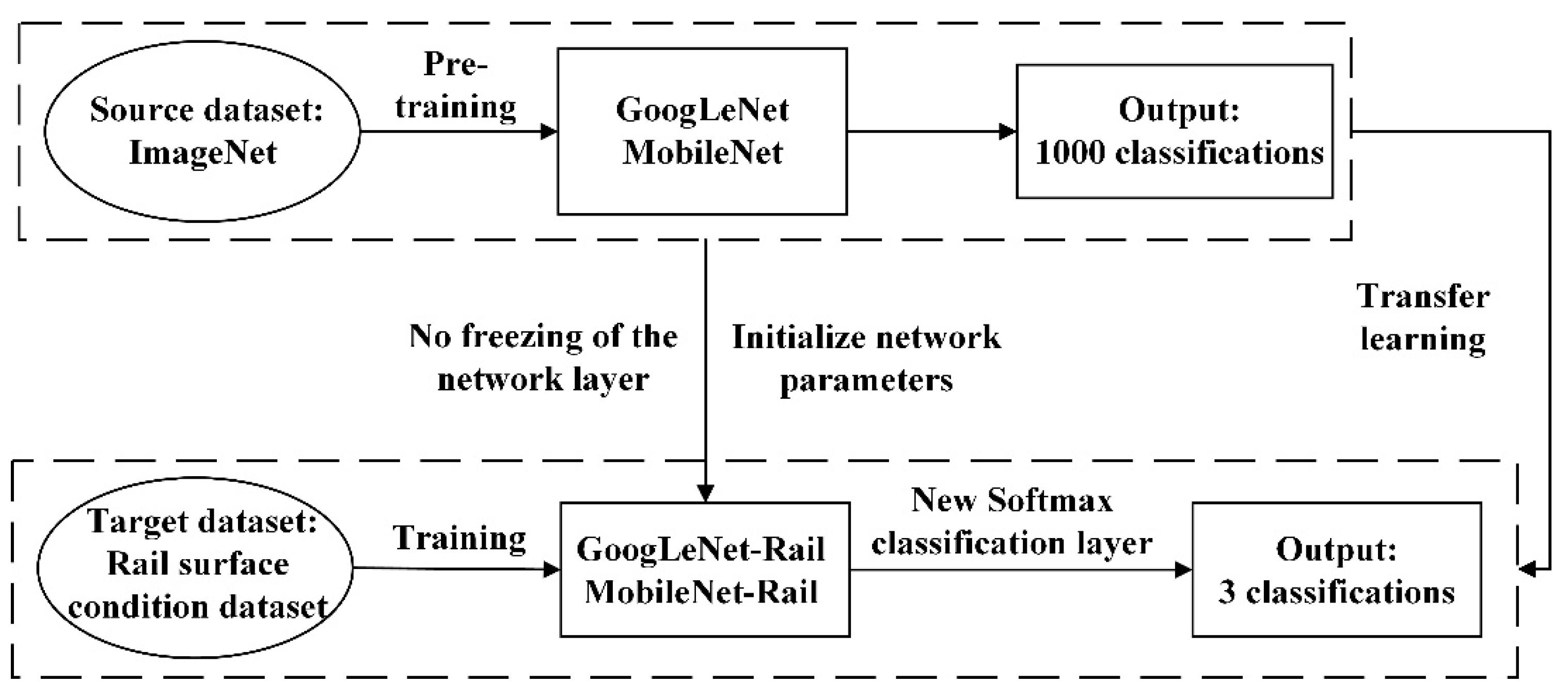
The implementation process begins with pre-training both GoogLeNet and MobileNet on the ImageNet dataset, followed by the transfer of their parameters to the rail surface condition identification task. Two target networks, GoogLeNet-Rail and MobileNet-Rail, are subsequently created by copying the structure and parameters of the pre-trained models, with the exception of the output layer. These networks are used as rail surface image feature extractors, and an output layer is added to match the number of categories in the rail surface condition dataset. The parameters of this output layer are initialized randomly. Finally, effective transfer learning is achieved by training the target networks, GoogLeNet-Rail and MobileNet-Rail, to learn features specific to rail surface condition images. The realization process is illustrated in Figure 3.

2.2.2. Optimization of the Lightweight Model Based on Knowledge Distillation

In the knowledge distillation process, the teacher model not only provides traditional label information but also conveys richer knowledge to the student model through intermediate-layer feature representations. Soft labels, which represent the probabilities of each category in the Softmax output layer, are introduced. These soft labels encompass both the true label information and additional implicit knowledge beyond the actual labels. Although the output of the Softmax layer contains substantial information—providing the probability values for the true labels as well as indicating which negative labels are closer to the true labels—when the entropy of the probability distribution is low, the entropy of the negative labels’ distribution also becomes small. In such cases, the hard label values may approach zero, rendering them ineffective as soft labels. To address this, a temperature coefficient ($T$) is typically introduced in the Softmax function, enhancing the influence of negative label information and facilitating the transfer of more comprehensive knowledge. The knowledge distillation process can be divided into the following two stages:

• Teacher model training phase. In this phase, the teacher model is trained until it achieves satisfactory performance, after which its training parameters are solidified. The teacher model then generates high-fidelity knowledge outputs, including soft labels and intermediate layer features, which are subsequently transferred to the student model during the distillation process.
• Student model training phase. In this phase, the student model optimizes its training process by utilizing the soft labels generated by the teacher model. The performance of both the teacher and student models is evaluated using the following distillation loss function when aligning the respective logical units:

$$L_{KD}\left(p\left(u,T\right),p\left(z,T\right)\right)=\sum _{i=0}^k-p_i\left(u_i,T\right)\mathit{log}\left(p_i\left(z_i,T\right)\right)$$

(1)

where $T$ is the temperature coefficient used to control the softening of the output probabilities, $u$ and $z$ are the logical units of the output of the teacher and student models, respectively, $u_i$ and $z_i$ are the values of the logical units of the $i$-th class of the teacher and student models, $p_i$ is the class probability of the $i$-th class, and $k$ denotes the category. When $T$ is positive infinity, the distillation loss at backpropagation is optimized as follows:

$$\begin{gathered} {\displaystyle \frac{\partial L_{KD}\left(p\left(u,T\right),p\left(z,T\right)\right)}{\partial z_i}}={\displaystyle \frac{p_i\left(z_i,T\right)-p_i\left(u_i,T\right)}{T}} \\ \approx {\displaystyle \frac{1}{T}}\left({\displaystyle \frac{1+\left(\frac{z_i}{T}\right)}{k+\sum _{j=0}^k\frac{z_i}{T}}}-{\displaystyle \frac{1+\left(\frac{u_i}{T}\right)}{k+\sum _{j=0}^k\frac{u_i}{T}}}\right) \end{gathered}$$

(2)

Assuming that $z_i$ is 0-mean, there is the following:

$${\displaystyle \frac{\partial L_{KD}\left(p\left(u,T\right),p\left(z,T\right)\right)}{\partial z_i}}\approx {\displaystyle \frac{1}{k{T}^2}}\left(z_i-u_i\right)$$

(3)

In addition to training with the soft labels generated by the teacher model, incorporating hard labels further enhances the learning process. This is achieved by balancing the contributions of two distinct objective functions. The first objective function represents the cross-entropy loss between the teacher model’s predictions at a higher temperature $T$ and the student model’s predictions at the same elevated $T$. The second objective function corresponds to the cross-entropy loss between the student model’s predictions and the ground-truth hard labels, computed at $T$ = 1. The total loss function is formulated as follows:

$$L_{total}=\lambda ·L_{KD}\left(p\left(u,T\right),p\left(z,T\right)\right)+\left(1-\lambda \right)·L_S\left(y,p\left(z,1\right)\right)$$

(4)

where $\mathsf{\lambda }$ is the hyperparameter and $L_S\left(y,p\left(z,1\right)\right)$ is the student loss, which is denoted as follows:

$$L_S\left(y,p\left(z,1\right)\right)=\sum _{i=0}^k-y_i\mathit{log}\left(p_i\left(z_i,1\right)\right)$$

(5)

where $\mathrm{y}$ is the vector of hard labels. Figure 4 illustrates the realization process.

2.2.3. Optimized Application of Mixed-Precision Training Strategies

To further enhance the computational efficiency of the model, this study employs a mixed-precision training strategy, integrating half-precision floating-point (FP16) and single-precision floating-point (FP32) arithmetic. This approach aims to accelerate computation while reducing memory consumption. During training, model weights are initialized using FP32 precision. In the forward propagation phase, most tensor computations are performed with FP16 precision, whereas loss calculations are retained in FP32 to ensure numerical accuracy and gradient stability. To mitigate potential gradient underflow issues associated with FP16 precision, a loss scaling mechanism is introduced. Prior to gradient computation, the loss value is scaled by a fixed scaling factor (Loss Scale) to preserve numerical precision. During backpropagation, the majority of gradient computations are conducted in FP16 precision, facilitating faster training and lower memory overhead. Subsequently, at the end of backpropagation, the computed gradients are rescaled by the Loss Scale factor to restore their original range. Finally, weight updates are applied in FP32 precision using the optimizer. In cases where gradient overflow is detected, the corresponding weight update step is skipped to maintain training stability. The implementation process is illustrated in Figure 5.

2.3. Fuzzy Fusion Estimation Module

To enable the practical application of rail surface condition identification in adhesion control, this study proposes a multi-source information fusion mechanism that integrates train operation data with rail surface condition identification. This approach aims to characterize rail surface adhesion conditions more comprehensively and enhance the robustness of maximum adhesion coefficient estimation. Since the adhesion state between the wheels and rails during train operation is difficult to represent by an accurate mathematical model, fuzzy control is appropriate, and fuzzy control enables the effective integration of multiple types of information. The fuzzy control method is employed to fuse multimodal input information, selecting four representative rail surface states as standard conditions to encompass a wide range of operational scenarios. These standard rail surfaces are used to derive adhesion coefficient creep and slide speed curves. In real-world train operations, the actual adhesion characteristic curve does not precisely coincide with any single standard rail surface curve. Instead, it typically lies near one or multiple standard curves, indicating varying degrees of similarity between the actual rail surface and the predefined standard surfaces. To account for this, the adhesion coefficient estimated by the full-dimensional state observer and creep and slide speed are utilized as inputs, which are first fuzzified and subsequently compared against the four standard adhesion curves. Following defuzzification, four similarity scores are obtained, representing the degree of correlation between the current rail surface and each standard condition. These similarities are then used as weighting coefficients in a weighted average calculation to estimate the maximum adhesion coefficient, as expressed in Equation (6). To further refine this estimation, rail surface condition information is incorporated to adjust the four similarity scores. Through fuzzy logic control, correction values are computed and applied to the initial similarities. The adjusted similarity scores are then used as weighting coefficients in a second weighted average computation, yielding the final maximum adhesion coefficient after multi-source information fusion. The corresponding formula is presented in Equation (7).

$${\mu }_{max}={\displaystyle \frac{{\sum }_{i=1}^4{x}_i{\mu }_{maxi}}{{\sum }_{i=1}^4{x}_i}}$$

(6)

where ${\mu }_{max}$ corresponds to the maximum adhesion coefficient of the four standardized rail surfaces and $x_i$ corresponds to the similarity between the rail surfaces and the four standardized rail surfaces. ${\mu }_{maxi}$ corresponds to the value of the maximum adhesion coefficient of the standard rail surface $i$.

$${\mu }_{max}={\displaystyle \frac{\sum _{i=1}^4{k}_i{x}_i{\mu }_{maxi}}{\sum _{i=1}^4{k}_i{x}_i}}$$

(7)

where $k_i$ corresponds to the rail surface condition correction factor.

2.3.1. Fuzzy Controller Design Ideas for Unintegrated Rail Surface Conditions

The real-time calculated creep–slip velocity and the adhesion coefficient estimated by the observer serve as the two input variables, while the similarity between the current rail surface and the four predefined standard rail surfaces $x_1$, $x_2$, $x_3$, and $x_4$ constitute the four output variables. To establish a structured classification, the adhesion characteristic curves of the four standard rail surfaces are analyzed, and the creep–slip velocity is categorized into three levels based on the density distribution of the curves: large creep, medium creep, and small creep. Similarly, the adhesion coefficient is classified into four fuzzy subsets, denoted as 1, 2, 3, and 4, each corresponding to a specific standard rail surface. The similarity measure between the current rail surface and each standard rail surface is also divided into four fuzzy subsets: very similar, similar, generally similar, and not similar. These fuzzy values are then converted into precise numerical values using the center of area defuzzification method. The rules governing the fuzzy controller are systematically organized and presented in

Table 1. Table of logical inference rules for unintegrated rail surface states.

Input Quantity		Output Quantity
Creep and Slide Speed	Adhesion Coefficient	${\mathit{x}}_1$	${\mathit{x}}_2$	${\mathit{x}}_3$	${\mathit{x}}_4$
Small	1	Very similar	Similar	Not similar	Not similar
Small	2	Similar	Very similar	Generally similar	Not similar
Small	3	Not similar	Generally similar	Very similar	Similar
Small	4	Not similar	Not similar	Similar	Very similar
Medium	1	Very similar	Generally similar	Not similar	Not similar
Medium	2	Similar	Very similar	Generally similar	Generally similar
Medium	3	Not similar	Similar	Very similar	Similar
Medium	4	Not similar	Generally similar	Similar	Very similar
Large	1	Very similar	Generally similar	Not similar	Not similar
Large	2	Generally similar	Very similar	Generally similar	Not similar
Large	3	Not similar	Generally similar	Very similar	Similar
Large	4	Not similar	Not similar	Generally similar	Very similar

.

2.3.2. Fuzzy Controller Design Ideas for Integrated Rail Surface Conditions

The rail surface condition (dry, wet, oil contaminated), the ratio of the similarity between the current rail surface and standard rail surface 1 to the sum of all similarities ($u_1$), and the ratio of the similarity between the current rail surface and standard rail surface 4 to the sum of all similarities ($u_4$) are selected as the three input variables. The four outputs are the correction coefficients ($k_1$, $k_2$, $k_3$, $k_4$) for the similarity values, adjusted based on the identified rail surface condition. The values of $u_1$ and $u_4$ are used to determine which standard rail surface the current rail surface is more closely associated with. If the identified bias differs across standard rail surfaces, the corresponding correction coefficients will also vary accordingly, enhancing the robustness of the system. Among these inputs, the rail surface condition is a categorical state variable, while $u_1$ and $u_4$ are continuous numerical values. To align with fuzzy logic processing, $u_1$ and $u_4$ must be fuzzified before logical inference. The rail surface condition is classified into three discrete states: dry, wet, and oil contaminated. The values of $u_1$ and $u_4$ are divided into five fuzzy levels: very large, large, medium, small, and very small. The correction coefficients for rail surface conditions are categorized into four fuzzy subsets: decreased, unchanged, increased, and significantly increased. The inclusion of the “significantly increased” subset accounts for the fact that oil contamination has a more severe impact on adhesion compared to wet conditions. Consequently, when the rail surface is identified as oil contaminated, a larger correction factor is applied. The fuzzy control rules governing these corrections are presented in

Table 2. Table of logical inference rules for integrated rail surface states.

Input Quantity			Output Quantity
Rail Surface Condition	${\mathit{u}}_1$	${\mathit{u}}_4$	k1	k2	k3	k4
Dry	Very small	-	decrease	unchange	unchange	increase
Dry	Small	-	unchange	unchange	unchange	increase
Dry	Medium	-	increase	unchange	unchange	unchange
Dry	Large	-	increase	unchange	unchange	unchange
Dry	Very large	-	increase	increase	unchange	decrease
Wet	Very small	-	decrease	unchange	unchange	increase
Wet	Small	-	decrease	unchange	unchange	increase
Wet	Large	-	increase	unchange	unchange	unchange
Wet	Very large	-	increase	unchange	unchange	unchange
Wet	-	Very small	increase	unchange	unchange	unchange
Wet	-	Small	unchange	unchange	increase	unchange
Wet	-	Large	unchange	unchange	unchange	increase
Wet	-	Very large	decrease	decrease	unchange	increase
Oil	-	Very small	increase	unchange	unchange	unchange
Oil	-	Small	unchange	unchange	significantly increase	unchange
Oil	-	Medium	unchange	unchange	significantly increase	significantly increase
Oil	-	Large	decrease	unchange	significantly increase	significantly increase
Oil	-	Very large	decrease	decrease	significantly increase	significantly increase

.

3. Experimental Results and Analysis

3.1. Dataset and Evaluation Indicators

Modern trains are typically equipped with a front-facing camera positioned in the driver’s cabin to monitor the external environment and rail conditions in real time, providing a 180-degree field of view. However, due to the high installation position and wide field of view, accurately identifying the rail surface condition remains challenging. To address this issue, this study proposes a custom data acquisition platform based on a typical industrial machine vision system, as illustrated in Figure 6. The dataset used for testing was partially collected from the railroad section and partially from the Central South University railroad test section. To ensure high-quality image acquisition under varying conditions, an industrial camera is securely mounted on a rocker arm, which is fixed to the platform. Considering the complexity of the actual train operating environment, image data collected across different time periods, varying lighting conditions, diverse weather states, and different operating speeds are incorporated into the data acquisition process. This approach enhances the diversity and representativeness of the dataset, thereby improving the model’s robustness and generalization ability in complex scenarios. The industrial camera has a resolution of 1920 × 1080, and the mounting height is set to 1 m.

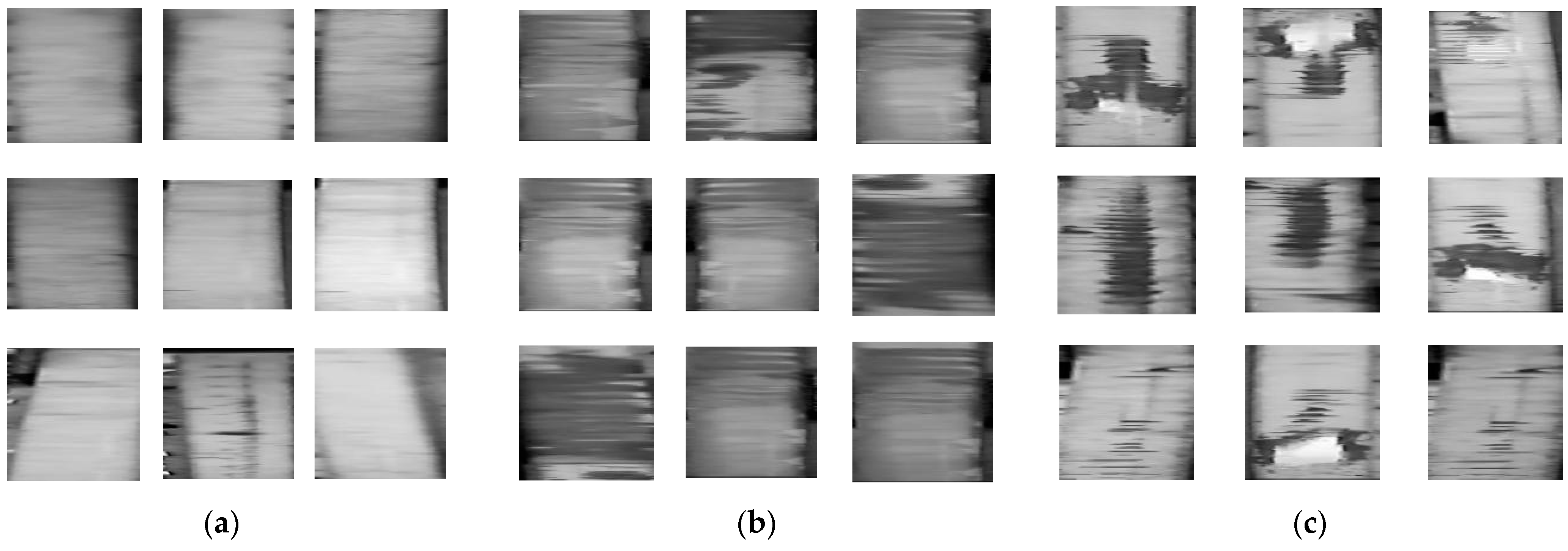
The dataset collected for this study consists of 1500 images for each of the three rail surface conditions: dry, wet, and oil contaminated. After undergoing a series of pre-processing steps, including grayscale conversion, denoising, enhancement, perspective transformation, rail surface area extraction, and data augmentation (brightness enhancement, brightness reduction, horizontal mirroring, vertical mirroring, picture rotation), the dataset was expanded to a total of 31,500 images, comprising 10,500 images for each rail surface condition. To establish a standardized image database, all images were resized to 224 × 224 pixels, ensuring consistency in data representation. The dataset was then partitioned into training, validation, and test sets at a ratio of 6:2:2 for each category. Figure 7 presents sample images from the dataset. The training set and validation set are utilized for model training and hyperparameter tuning, while the test set is employed to assess the generalization ability of the final model. The evaluation metrics include accuracy, precision, recall, F1 score, model inference time, and the number of parameters. Accuracy refers to the ratio of correctly classified samples to the total number of samples. Precision measures the proportion of true positive cases among all samples predicted as positive, while recall reflects the proportion of actual positive cases that are correctly identified. The F1 score is the harmonic mean of precision and recall. These four metrics allow for a comprehensive evaluation of model recognition performance. Additionally, model inference time and the number of parameters serve as indicators for assessing the real-time performance and lightweight characteristics of the model.

3.2. Experimental Environment and Parameter Settings

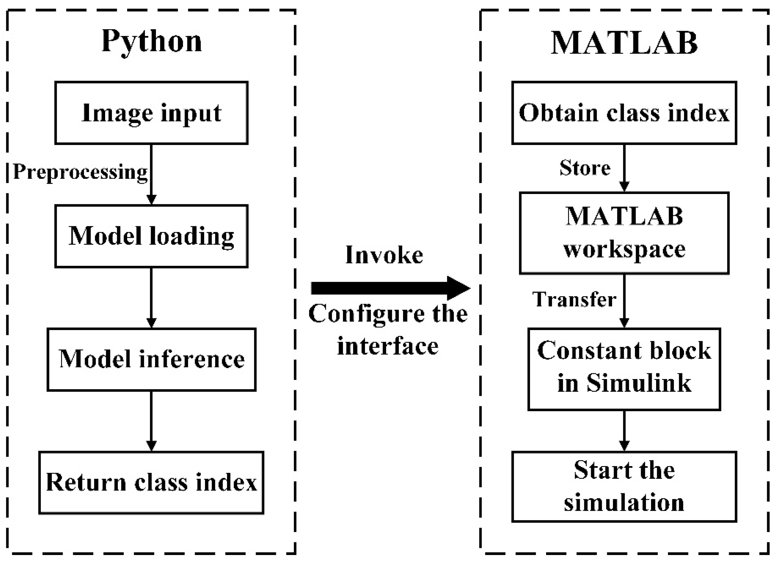
Experimental hardware platform. The operating system is Windows 10-64 bit, the CPU is an 11th Gen Intel(R) Core(TM) i7-11800H@2.30 GHz (16 CPUs)~2.3 GHz, GPU 0 is an Intel(R) UHD Graphics, and GPU 1 is an NVIDIA GeForce RTX 3060 Laptop GPU. The software platform is Python 3.9.0 (64-bit), PyCharm Community Edition 2022.1.3, which is used to build the deep learning framework. Simulink in MATLAB R2023b is used to build the traction dynamics model. The interface between Python and MATLAB should be configured with particular attention to ensure compatibility between the two versions. In Python, the rail surface condition identification model, which has been developed, is loaded to recognize images and output class index values. These values are then called by MATLAB through the py function and stored in the MATLAB workspace. Subsequently, the set_param() function is used to transfer the stored values from the workspace to the Constant block within the Simulink model, where they serve as inputs to the traction dynamics model. This process facilitates the integration of both Python and MATLAB for co-simulation. A detailed flowchart of this procedure is shown in Figure 8. When the rail surface condition identification model is trained, the learning rate of the experiment is set to 1 × 10⁻⁵, the batch size is set to 64, and the number of training rounds is set to 100 epoches. A smaller learning rate helps avoid oscillations or divergence during model training, batch size 64 provides a better balance between training stability and computational efficiency, and 100 epoches gives the model ample time to train. The classification function uses the Softmax function, the loss function uses the cross-entropy function, and the default framework parameters of the adaptive learning rate optimization algorithm Adam are used. These three are the classical configurations in deep learning classification tasks.

3.3. Validation of the Effectiveness of the Rail Surface Condition Identification Algorithm

3.3.1. Validation of the Effectiveness of Transfer Learning

To evaluate whether transfer learning enhances the training performance of both the teacher model and the student model, Group 1 ablation experiments were conducted. The validation set accuracy and loss for both models, before and after applying transfer learning, are illustrated in Figure 9. Model performance was further assessed on the test set, with key evaluation metrics summarized in

Table 3. Results of the transfer learning experiment.

Model	Accuracy/%	Precision/%	Recall/%	F1/%	Model Inference Time/s	Number of Parameters/106
GoogLeNet	96.05	96.15	96.05	96.05	0.0404	6.62
GoogLeNet-Rail	96.90	96.93	96.90	96.91	0.0422	5.60
MobileNet	86.89	88.66	86.89	86.96	0.0402	5.48
MobileNet-Rail	95.40	95.58	95.40	95.38	0.0397	4.21

. The results demonstrate that transfer learning significantly accelerates network convergence and improves accuracy. This improvement is attributed to the pre-trained model initialization, which allows the earlier layers of the network to inherit well-optimized parameters, bringing them closer to the optimal solution early in the training process. Additionally, since all layers undergo transfer learning, the model can extract finer-grained feature details from images, leading to higher identification accuracy. A comparative analysis between the GoogLeNet (teacher) model and the MobileNet (student) model further confirms that both models exhibit substantial performance improvements after applying transfer learning. In terms of loss convergence, both GoogLeNet and MobileNet demonstrate enhanced learning capabilities following transfer learning. The models subjected to transfer learning exhibit a lower initial loss value, with a rapid decline and faster stabilization. In contrast, models without transfer learning present a higher initial loss and experience significantly greater fluctuations throughout the training process. Regarding evaluation metrics, including accuracy, precision, recall, and F1 score, GoogLeNet and MobileNet after transfer learning outperform their counterparts without transfer learning. Notably, MobileNet shows a more pronounced optimization effect. This is further corroborated by the accuracy curve, which indicates reduced accuracy fluctuations and improved feature extraction from the dataset. In terms of inference time, the difference between GoogLeNet and MobileNet after transfer learning is either minimal or shorter. Specifically, MobileNet achieves a 1.24% reduction in inference time. Although the reduction is relatively modest, the simultaneous improvement in accuracy underscores the effectiveness of transfer learning. Furthermore, the number of parameters in both GoogLeNet and MobileNet is significantly reduced after transfer learning. GoogLeNet experiences a 15.41% reduction in parameter count, while MobileNet achieves a 23.18% reduction. This reduction in parameters further enhances the model’s lightweight nature, contributing to improved efficiency and performance.

3.3.2. Validation of the Effectiveness of Knowledge Distillation

To assess whether knowledge distillation enhances the identification accuracy of the lightweight model and improves overall model performance, a Group 2 ablation experiment was conducted. In this experiment, the GoogLeNet-Rail model was utilized as the teacher model to guide the MobileNet-Rail model (student model), transferring learned feature knowledge through the distillation process. A critical parameter in knowledge distillation is the distillation temperature ($T$), which significantly influences the student model’s learning effectiveness. To investigate its impact, experiments were conducted with different temperature values, and the results are presented in

Table 4. Experimental results for different distillation temperatures in the student model MobileNet-Rail.

$\mathbf{T}$	Accuracy/%	Precision/%	Recall/%	F1/%	Model Inference Time/s
1	94.78	95.02	94.78	94.76	0.0385
2	95.35	95.49	95.35	95.35	0.0384
3	95.30	95.53	95.30	95.28	0.0383
4	95.97	96.12	95.97	95.96	0.0382
5	97.10	97.16	97.10	97.10	0.0380
10	97.11	97.17	97.11	97.12	0.0379
20	97.08	97.17	97.08	97.07	0.0381

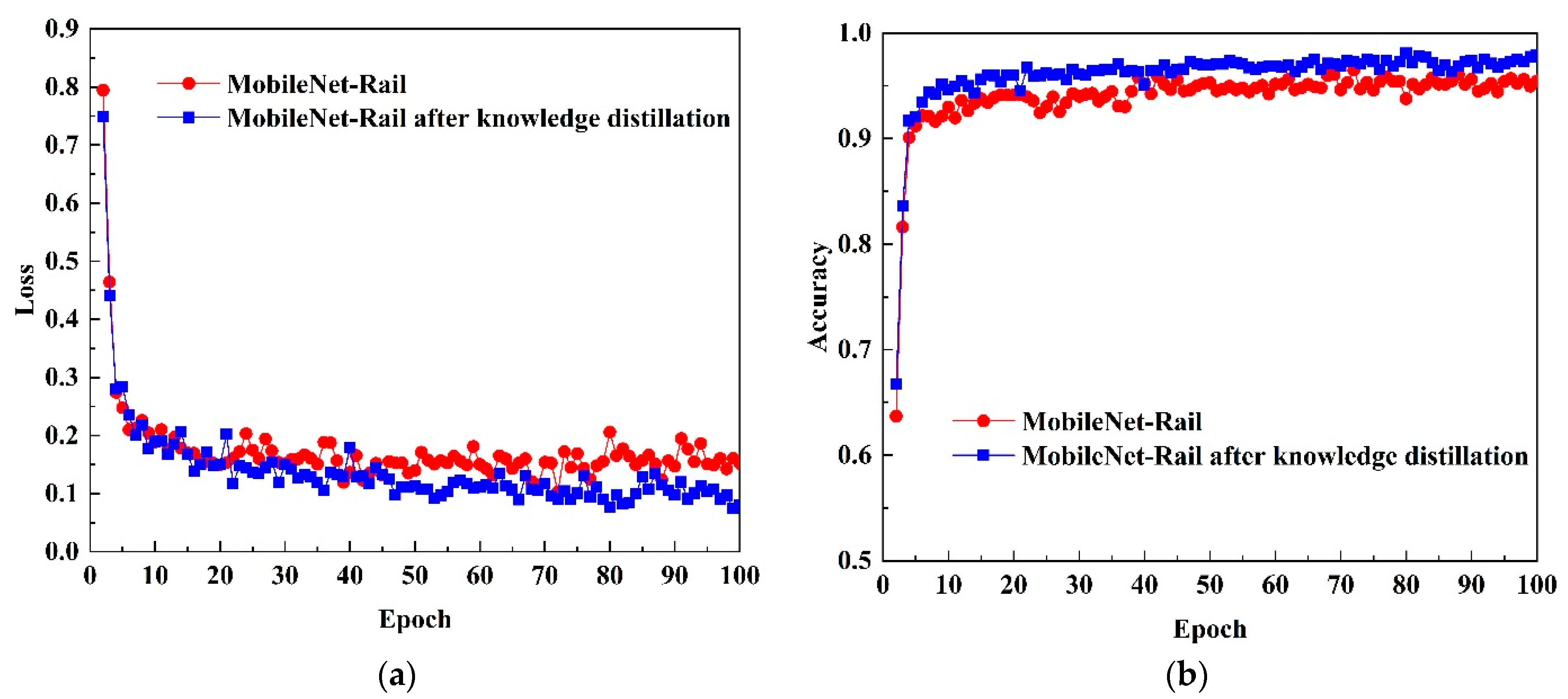
. The highest identification accuracy of 97.11% was achieved at a distillation temperature of 10. Furthermore, the performance comparison of the student model with and without knowledge distillation, specifically at $T$ = 10, is illustrated in Figure 10. According to the experimental results, it is evident that the loss values of MobileNet-Rail are lower and exhibit reduced fluctuation after knowledge distillation. Moreover, the accuracy, precision, recall, and F1 score are all enhanced, while the inference time is slightly reduced. The optimal performance is achieved when the distillation temperature is set to 10. In summary, the knowledge distillation effectively enhances the identification capability of the student model, improving its classification performance. Notably, at an appropriate distillation temperature, the student model’s accuracy can match or even surpass that of the teacher model.

3.3.3. Validation of the Effectiveness of Mixed-Precision Training

To evaluate whether mixed-precision training enhances the computational efficiency of the model, a third group of ablation experiments was conducted. In this experiment, mixed-precision training was applied to the MobileNet-Rail model trained with knowledge distillation. The objective was to compare the model inference time and classification accuracy between full-precision training and mixed-precision training, with the results presented in

Table 5. Mixed-precision training test results.

Mixed-Precision Training	Accuracy/%	Model Inference Time/s
×	97.11	0.0379
√	97.38	0.0371

. The experimental findings indicate that mixed-precision training significantly improves computational efficiency, reducing model inference time while maintaining the classification performance of the original model. This demonstrates that mixed-precision training is an effective technique for optimizing deep learning models, enabling faster inference without compromising accuracy.

3.3.4. Comparison with Other Algorithms

To further evaluate the effectiveness of the proposed model, mainstream image classification networks were compared using the same dataset and under identical experimental conditions. The models selected for comparison include AlexNet [21], VGG16 [22], GoogLeNet [19], ResNet18 [23], ResNet34 [23], ResNet50 [23], EfficientNet [14], ShuffleNet [12], and MobileNet [13]. Since GoogLeNet and MobileNet were used as the teacher and student models in the previous experiments, their performance without transfer learning was also included for reference. The evaluation results of all models in the test set are shown in

Table 6. Performance of each model and experimental results.

Model	Accuracy/%	Precision/%	Recall/%	F1/%	Model Inference Time/s	Number of Parameters/106
AlexNet	86.37	86.26	86.37	86.23	0.0346	61.10
VGG16	91.46	91.91	91.46	91.51	0.0361	138.36
GoogLeNet	96.05	96.15	96.05	96.05	0.0404	6.62
ResNet18	94.38	94.42	94.38	94.38	0.0334	11.69
ResNet34	95.97	96.07	95.97	95.97	0.0347	21.80
ResNet50	91.75	92.18	91.75	91.78	0.0382	25.56
EfficientNet	84.81	87.08	84.81	84.92	0.0440	5.29
ShuffleNet	82.78	84.37	82.78	82.84	0.0478	1.37
MobileNet	86.89	88.66	86.89	86.96	0.0402	5.48
Ours	97.38	97.42	97.38	97.39	0.0371	4.21

. From the accuracy results, among the non-lightweight models, GoogLeNet achieved the highest accuracy, followed by the ResNet series. AlexNet had the lowest accuracy, suggesting that deeper networks are better at capturing complex features. Among the lightweight models, the accuracy of all lightweight models was lower than that of non-lightweight models, likely due to shallower network depth and reduced feature extraction capabilities. MobileNet outperformed other lightweight models, confirming its suitability for the student model in the knowledge distillation strategy. The proposed model achieved the highest accuracy of 97.38%, surpassing other models by 1.4% to 17.6%, a model inference time of only 0.0371 s, ranking in the mid-to-upper range among all networks, and a parameter size of 4.21 × 10⁶, which is significantly smaller than GoogLeNet and ResNet models while maintaining comparable performance. Considering all evaluation metrics, the lightweight rail surface condition identification model based on knowledge distillation and transfer learning achieves the best balance between accuracy, efficiency, and real-time performance. This makes it suitable for deployment on trains, ensuring high identification accuracy while maintaining the real-time processing requirements of onboard systems.

Furthermore, compared to the model in the literature [11], which shares the same recognition task and exhibits similar rail surface condition characteristics, the proposed model in this paper achieves a significant reduction in the number of parameters, a slight improvement in recognition accuracy, and enhanced suitability for vehicle deployment, making it more practical for real-world applications.

3.4. Experiments on Maximum Adhesion Coefficient Estimation

In this experiment, the train traction dynamics simulation model is built using the parameters of the HXD1 (23t) locomotive. The train running resistance is expressed in terms of unit basic resistance, which is determined using a characteristic formula. To allow for experimental adjustments, multiple traction levels are set. Additionally, four standard rail surfaces are established as benchmarks for subsequent similarity determination in the fuzzy control system. Based on the density distribution of the adhesion characteristic curves corresponding to these four standard rail surfaces, as well as the specific experimental conditions, the affiliation functions for each input and output variable of the fuzzy controller are carefully defined.

3.4.1. Acquisition of Standard Rail Surface Curves

The relationship between the wheel–rail adhesion coefficient and creep–slip velocity is expressed in Equation (8). Based on previous experimental studies, four different rail surface conditions are selected as the standard rail surfaces for this study [24]. The four standard rail surfaces correspond to dry, wet, snowy, and oily rail surface conditions in that order. The adhesion characteristic parameters (a, b, c, d values) for each rail surface are provided in

Table 7. Table of values for standard rail surface parameters.

Rail Surface Condition	a	b	c	d	${\mathit{\mu }}_{\mathit{m}\mathit{a}\mathit{x}}$
Track 1	0.54	1.20	1.20	1.20	0.343
Track 2	0.27	0.83	0.50	0.50	0.197
Track 3	0.19	0.54	0.40	0.40	0.147
Track 4	0.09	0.54	0.20	0.20	0.117

, while the corresponding adhesion characteristic curves are illustrated in Figure 11.

$$\mu =c{e}^{-a{v}_s}-d{e}^{-b{v}_s}$$

(8)

3.4.2. Setting of the Affiliation Function

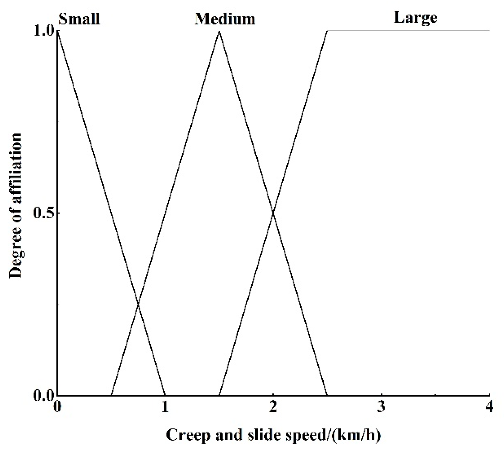
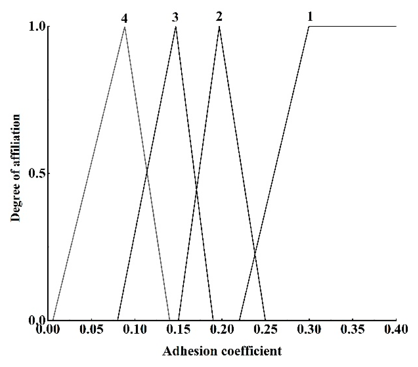
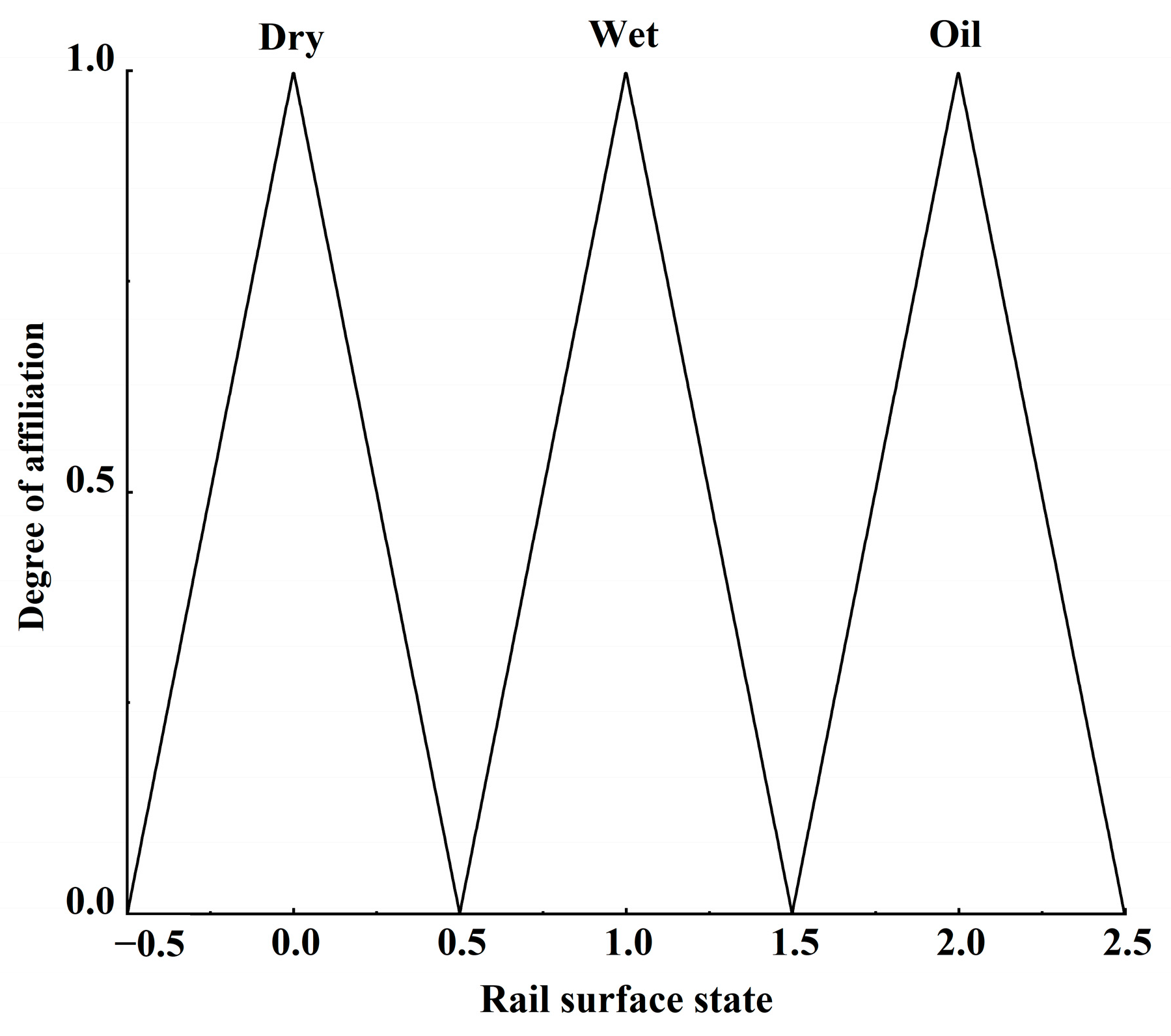
The affiliation functions to be set include creep and slide speed affiliation function, adhesion coefficient affiliation function, similarity affiliation function, rail surface condition affiliation function, ${\mathrm{u}}_1$ and $u_4$ affiliation function, and rail surface condition correction coefficient affiliation function. Analyzing the four adhesion characteristic curves in Figure 11, it can be seen that when the creep and slide speed is below 1 km/h or above 2.5 km/h, the distribution of the four curves is denser, with less differentiation, according to which the affiliation function of creep and slide speed is set up; the affiliation function of the rail surface condition is set up according to the state quantity recognized by the identification module, and the other affiliation functions are dynamically adjusted according to the experimental specific conditions. The affiliation function diagrams are shown in Figure 12, Figure 13, Figure 14, Figure 15, Figure 16 and Figure 17. 1–4 in Figure 13 correspond to the four standard rail surfaces.

3.4.3. Simulation of Maximum Adhesion Coefficient Estimation

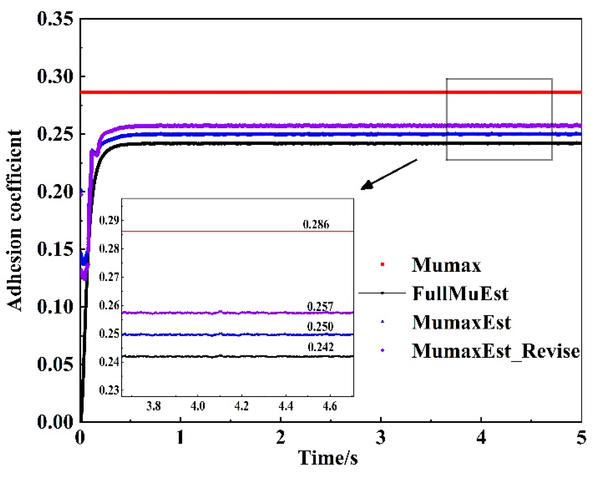
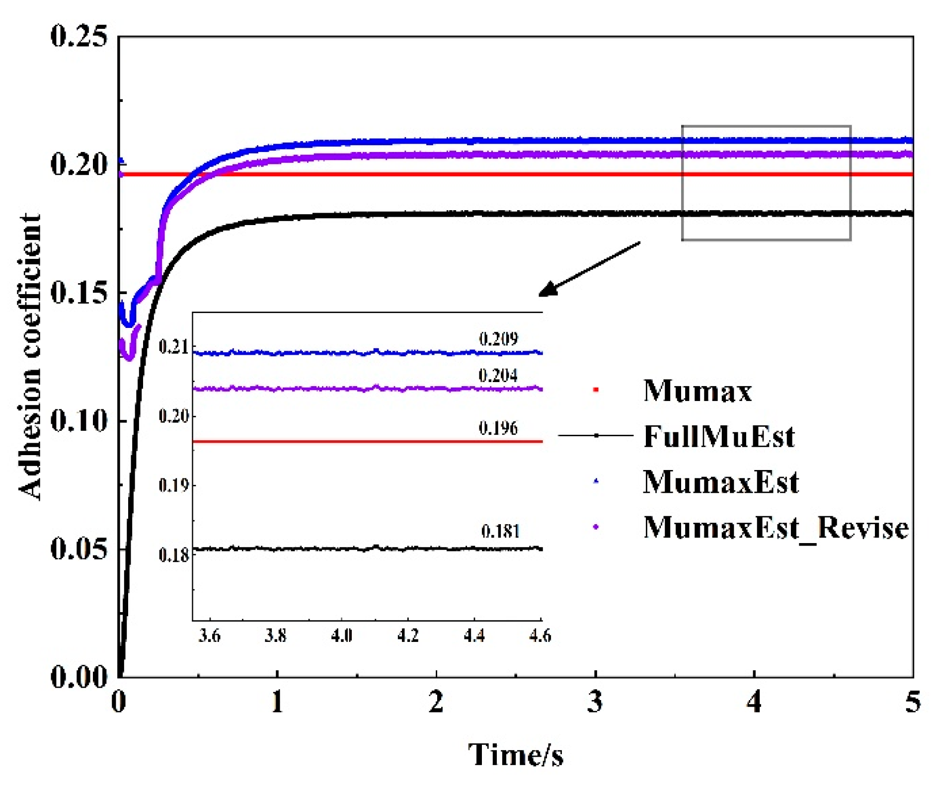
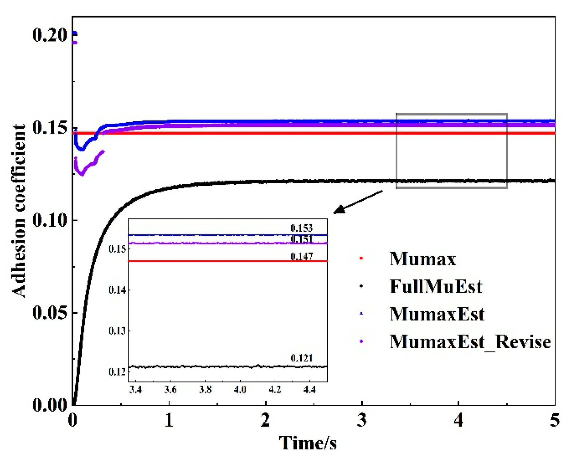
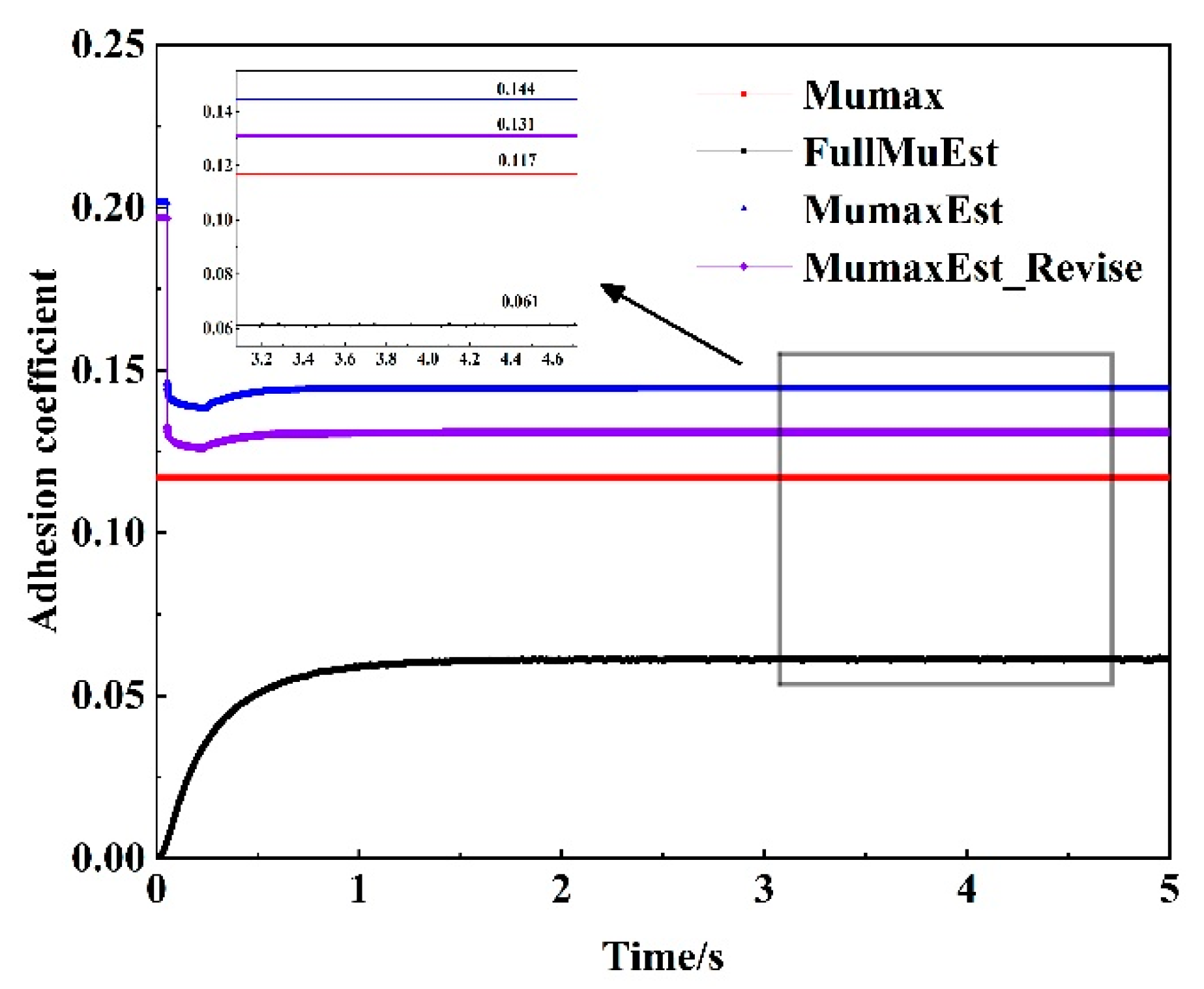
Four rail surface conditions, dry, wet, snowy, and oily rails, were selected as the simulated rails. The maximum adhesion coefficients of the four rail conditions match the experimental range of the UIC ORE B44 committee, and the maximum adhesion coefficients (ideal values) are 0.286, 0.197, 0.147, and 0.117. To emphasize the effectiveness of the proposed method, the traction level was set to a lower value for each rail condition, resulting in a certain gap between the actual adhesion coefficient and the ideal maximum adhesion coefficient. This setup allows for comparison of the estimated maximum adhesion coefficient with the ideal value, thus testing the precision of the estimation process. During the experiment, the time of rail surface image identification is considered negligible to focus on the performance of the adhesion coefficient estimation. The main discussion is about several common cases. Combinations of simulated rail and the recognized rail surface conditions include “dry + dry”, “wet + wet”, “snowy + wet”, and “oily + oil”. The experimental results are shown in Figure 18, Figure 19, Figure 20 and Figure 21, where the following comparisons are made: ideal maximum adhesion coefficient, estimated maximum adhesion coefficient for unfused rail surface conditions, and estimated maximum adhesion coefficient for fused rail surface conditions.

Where Mumax is the ideal maximum adhesion coefficient, FullMuEst is the real-time adhesion coefficient estimated by the full-dimensional state observer, MumaxEst is the maximum adhesion coefficient estimated using the fuzzy control strategy, and MumaxEst_Revise is the corrected maximum adhesion coefficient, incorporating rail surface condition information. Under the simulation conditions designed in this study, the estimation error of the dry simulation rail is reduced from 12.6% to 10.1%, the estimation error of the wet simulation rail is reduced from 6.7% to 4.1%, the estimation error of the rainy and snowy simulation rail is reduced from 4.1% to 2.7%, and the estimation error of the oiled simulation rail is reduced from 23.1% to 12.0%. These results indicate that incorporating rail surface conditions improves the accuracy of the maximum adhesion coefficient estimation, effectively reducing estimation errors across different rail conditions and their various combinations. This is particularly crucial under complex operating conditions. In comparison with the maximum adhesion coefficient estimation method presented in the literature [24] under identical experimental conditions, the approach in the literature [24] does not incorporate rail surface conditions, relying solely on the adhesion coefficient and creep and slide speed (i.e., the MumaxEst values shown in Figure 18, Figure 19, Figure 20 and Figure 21). In contrast, the method proposed in this paper, by integrating critical environmental information, can better adapt to changes in the environment, thereby improving estimation accuracy. Furthermore, this approach provides reliable operational condition awareness, which can enhance the effectiveness of adhesion control strategies and improve the safety of train operations.

4. Conclusions

Aiming at the engineering problems of a large number of parameters, high computational delay, and difficulty in realizing onboard deployment of the current rail surface state identification model, this paper proposes a lightweight rail surface state identification method for estimating the maximum adhesion coefficient of the wheel–rail, which can improve the traction and braking efficiency of the train by accurately identifying the rail surface state in front of the rail, integrating this state information into the framework of estimating the maximum coefficient of the wheel–rail, and then providing the threshold value of the maximum coefficient of adhesion for the optimal adhesion control. The conclusions are as follows:

(1)

The lightweight rail surface condition identification model proposed in this paper, based on knowledge distillation and transfer learning, effectively meets the practical requirements for high accuracy, low latency, and strong generalization in rail surface state recognition tasks. By employing GoogLeNet as the teacher model and MobileNet as the student model, the domain adaptation capability is enhanced through transfer learning. Additionally, the knowledge distillation strategy allows the student model to inherit knowledge from the teacher model, thereby reducing the number of parameters while maintaining accuracy. Furthermore, the introduction of mixed-precision training during the training process further reduces inference latency. The experimental results demonstrate that the proposed model achieves a size of only 4.21 MB, a test set accuracy of 97.38%, and an inference time of 0.0371 s, showcasing excellent overall performance and meeting the expected objectives.

(2)

The multi-source information fusion strategy designed in this paper can realize the fusion of rail surface condition information and maximum adhesion coefficient estimation. Through the design of a reasonable fuzzy control strategy, the train operation information is fuzzified and then compared with the set standard rail surface curve, and the similarity with the standard rail surface is obtained after anti-fuzzification. On this basis, the similarity is corrected by incorporating the rail surface condition information, and the corrected similarity is weighted as a weighting coefficient with the maximum adhesion coefficient value of the standard rail surface, and the maximum adhesion coefficient available for the current rail surface is calculated. The experimental results prove that the method can improve the estimation accuracy under arbitrary rail conditions, and the estimation error of a dry simulation track is reduced from 12.6% to 9.8%, the estimation error of a wet simulation track is reduced from 6.7% to 4.1%, the estimation error of a rainy and snowy simulation track is reduced from 4.1% to 2.7%, and the estimation error of an oily simulation track is reduced from 23.1% to 12.0%, which can provide a more accurate and precise maximum adhesion coefficient for optimal adhesion control and a more accurate threshold value for the maximum adhesion coefficient.

Although this study has achieved preliminary results, there is still much room for improvement. The rail surface condition information obtained in this paper should be the environmental information in front of the train operation; it takes some time for the wheel–rail to run to the front, and the data transmission will also lead to time delay. Therefore, there exists an unsynchronized information between the recognized rail surface condition and the environment where the train is actually located. Although the time is very short, the problem of spatial and temporal synchronization still needs to be taken into account; the currently used rail surface condition dataset lacks the categories of icy and snowy rail surfaces, water and oil mixed rail surfaces, and wet leafy rail surfaces, which need to be further expanded to make the algorithm more extensive. Due to experimental constraints, the proposed method has not yet been validated through real-world train experiments. In future work, real-world testing will be conducted to further assess the practical applicability of the proposed approach.

References

- Ohyama, T.; Nakano, S. Influence of surface contamination on adhesion force between wheel and rail at high speeds- behavior of adhesion force under the formation of lubricant film under the formation of lubricant film. J. Jpn. Soc. Lubr. Eng. 1989, 10, 121–124. [Google Scholar]
- Chang, C.; Chen, B.; Cai, Y.; Wang, J. Experimental Study on Large Creepage Adhesion of Wheel/RailBraking at 400 km ∙ h−1 (III)—Braking Adhesion Coefficient in Water Medium. China Railw. Sci. 2024, 45, 168–174. [Google Scholar]
- He, C.; Zhang, P.; Zou, G.; Song, Z.; Liu, J. Research progress on wheel-rail contact adhesion characteristic under environmental conditions. Tribology 2022, 42, 642–656. [Google Scholar]
- Chang, C.; Chen, B.; Cai, Y.; Wang, J. An Experimental Study of High Speed Wheel-rail Adhesion Characteristics in Wet Condition on Full Scale Roller Rig. Wear 2019, 440, 203092. [Google Scholar] [CrossRef]
- Wu, B.; Wen, Z.; Wang, H.; Jin, X. Analysis of wheel/rail adhesion under oil contamination with surface roughness. Proc. Inst. Mech. Eng. Part J J. Eng. Tribol. 2013, 227, 1306–1315. [Google Scholar] [CrossRef]
- Xu, K.; Xu, G.; Zheng, C. Novel determination of Wheel-Rail adhesion stability for electric locomotives. Int. J. Precis. Eng. Manuf. 2015, 16, 653–660. [Google Scholar]
- Xu, Q.; Cai, L. Active Braking Control of Electric Vehicles to Achieve Maximal Friction Based on Fast Extremum-Seeking and Reachability. IEEE Trans. Veh. Technol. 2020, 69, 14869–14883. [Google Scholar] [CrossRef]
- Bauer, J.; Pichlík, P.; Pavelka, J.; Zoubek, O.; Koucký, L.; Lev, M.; Zdeněk, J. A Method for Estimating the Slope of Adhesion of a Rail Vehicle at a Working Point and Apparatus for the Method: CZ2019-526. Patent CZ2019-526A3, 16 March 2025. [Google Scholar]
- Zhang, L.; Yu, L.; Wang, Z.; Zuo, L.; Song, J. All-Wheel Braking Force Allocation During a Braking-in-Turn Maneuver for Vehicles with the Brake-by-Wire System Considering Braking Efficiency and Stability. IEEE Trans. Veh. Technol. 2016, 65, 4752–4767. [Google Scholar]
- Miao, Y.; Ling, L.; Yang, Y.; Wang, K.; Zhai, W. Optimal Adhesion Control of High-speed Trains Based on Fuzzy Identification of Rail Surface Conditions. J. Mech. Eng. 2024, 1–10. Available online: http://kns.cnki.net/kcms/detail/11.2187.TH.20240925.1133.046.html (accessed on 16 March 2025).
- Yu, H.; Zhang, J.; Liu, J.; Peng, C.; Liu, L.; Gong, S. Rail surface condition recognition based on attention network and cost-sensitive learning under imbalanced data. Sci. Technol. Eng. 2024, 24, 1972–1979. [Google Scholar]
- Zhang, X.; Zhou, X.; Lin, M.; Sun, J. ShuffleNet: An Extremely Efficient Convolutional Neural Network for Mobile Devices. In Proceedings of the IEEE Conference on Computer Vision and Pattern Recognition (CVPR), Honolulu, HI, USA, 21–26 July 2017. [Google Scholar]
- Howard, A.G.; Zhu, M.; Chen, B.; Kalenichenko, D.; Wang, W.; Weyand, T.; Andreetto, M.; Adam, H. MobileNets: Efficient Convolutional Neural Networks for Mobile Vision Applications. arXiv 2017, arXiv:1704.04861. [Google Scholar]
- Tan, M.; Le, Q.V. EfficientNet: Rethinking Model Scaling for Convolutional Neural Networks. In Proceedings of the 36th International Conference on Machine Learning, Long Beach, CA, USA, 9–15 June 2019. [Google Scholar]
- Li, H.; Kadav, A.; Durdanovic, I.; Samet, H.; Graf, H.P. Pruning Filters for Efficient ConvNets. arXiv 2016, arXiv:1608.08710. [Google Scholar] [CrossRef]
- Zhou, S.; Wu, Y.; Ni, Z.; Zhou, X.; Wen, H.; Zou, Y. DoReFa-Net: Training Low Bitwidth Convolutional Neural Networks with Low Bitwidth Gradients. arXiv 2016, arXiv:1606.06160. [Google Scholar] [CrossRef]
- Zhu, C.; Han, S.; Mao, H.; Dally, W.J. Trained Ternary Quantization. arXiv 2016, arXiv:1612.01064. [Google Scholar] [CrossRef]
- Li, X.C.; Fan, W.S.; Song, S.; Li, Y.; Yunfeng, S.; Zhan, D.C. Asymmetric temperaturescaling makes larger networks teach well again. Adv. Neural Inf. Process. Syst. 2022, 35, 3830–3842. [Google Scholar]
- Szegedy, C.; Liu, W.; Jia, Y.; Sermanet, P.; Reed, S.; Anguelov, D.; Erhan, D.; Vanhoucke, V.; Rabinovich, A. Going Deeper with Convolutions. In Proceedings of the 2015 IEEE Conference on Computer Vision and Pattern Recognition (CVPR), Columbus, OH, USA, 23–28 June 2014. [Google Scholar] [CrossRef]
- Tan, C.; Sun, F.; Kong, T.; Zhang, W.; Yang, C.; Liu, C. A Survey on Deep Transfer Learning. In Artificial Neural Networks and Machine Learning; Springer: Cham, Switzerland, 2018. [Google Scholar] [CrossRef]
- Krizhevsky, A.; Sutskever, I.; Hinton, G. ImageNet Classification with Deep Convolutional Neural Networks. In Advances in Neural Information Processing Systems 25 (NIPS 2012); NIPS. Curran Associates Inc.: Red Hook, NY, USA, 2012. [Google Scholar] [CrossRef]
- Simonyan, K.; Zisserman, A. Very Deep Convolutional Networks for Large-Scale Image Recognition. arXiv 2014, arXiv:1409.1556. [Google Scholar] [CrossRef]
- He, K.; Zhang, X.; Ren, S.; Sun, J. Deep Residual Learning for Image Recognition. In Proceedings of the IEEE Conference on Computer Vision and Pattern Recognition (CVPR), Las Vegas, NV, USA, 27–30 June 2016. [Google Scholar] [CrossRef]
- Huang, J.; Tang, S.; Lin, P.; Ren, Q. Simulation Research on Locomotive Adhesion Control Based on Rail Identification. Comput. Simul. 2015, 32, 206–210+253. [Google Scholar]
Figure 1.
General architecture of the methodology.