Fibre Bragg Grating Wavelength Shift Demodulation with Filtering and Enhancement of Spectra by Simple Nonlinear Signal Processing

Featured Application

FBG sensors were used to measure temperature, stress, vibrations, and pressure. FBG sensors were used to monitor a variety of physical objects.

Abstract

A novel approach to fibre Bragg grating spectra processing is proposed. The method is based on the use of nonlinear filtration and raising the spectrum value to the second power. A combination of geometric and arithmetic mean filtering is used as nonlinear filtration. The properties of the denoising method are presented on simulation data with different signal-to-noise ratios and on experimental data. The most advantageous combination is raising the intensity of the spectrum to the square power preceded by its significant smoothing. The centroid, fast phase correlation, and cross-correlation methods are used to determine the wavelength shift in the spectrum. To obtain experimental data, measurements of the FBG in reflection mode placed in a temperature chamber with the possibility of temperature control are obtained. The simulations, measurements, and their numerical analysis confirm the usefulness of the proposed methods for demodulating the wavelength shift of FBG spectra.

1. Introduction

Fibre Bragg grating (FBG) sensors are used to measure various quantities such as temperature, stress, vibrations, pressure, or refractive index. The characteristic feature of these sensors is that the position of the spectrum changes due to the action of a particular physical quantity. FBGs are recorded in the fibre core, allowing all benefits associated with fibre optics to be applied, such as a small size or resistance to hazardous environments and electromagnetic interference. The determination of the Bragg wavelength change is an inherent aspect related to the use of Bragg grating sensors. In most cases, the developed methods are applied directly to the raw measured spectrum [1]. Some shift demodulation algorithms are involved in several methods that are used one after the other. The most important combination of algorithms is that of cross-correlation [2] with the Hilbert transformation [3]. Computationally efficient methods include the fast phase correlation algorithm [4], Karhunen–Loève transform (KLT) [5], second-order-polynomial-peak tracking [6], and representation of the measured spectrum using specific functions [7]. In the case of the demodulation of distorted spectra [8], the Gaussian curve fitting method [9] is effective. The most commonly used method, which can be described as preprocessing, is the wavelet transform. In its simplest form, this transform is used to filter the measured spectrum [10,11]. Classical digital filters were also applied to the FBG spectrum, which improved the accuracy of FBG sensors [12]. Several algorithms can be combined to remove noise from measurement data. An example of such solution is the decomposition of the FBG spectrum using ensemble empirical mode decomposition and filtering of the individual components using Savitzky–Golay filters [13]. A similar set of algorithms was used successively by [14]: variational mode decomposition, wavelet denoising, Hilbert transform, and the centroid algorithm. Recently, artificial neural network algorithms [15] and statistical methods [16] have also been used to demodulate FBG spectra. In this paper, we focus on the simultaneous filtration of and enhancement in FBG spectrum features based on the sum of the two elements’ products of the measured spectrum samples and raising the spectrum to the second power. As a starting methodology for consideration, we propose the use of the geometric mean as a signal smoothing filter. Then, we use modifications of the two-element geometric mean, which is the square root of the product of the current and previous spectrum samples. The modification consists of replacing the product of elements with an appropriate sum of two or more products. The subsequent factors of the individual products used contain samples that are separated (preceding and following) from the current sample by a certain distance (gap). As a comparative method for the proposed filtration method, the popular Savitzky–Golay filters were used.

2. Combining Geometric and Arithmetic Mean as a Denoising Method

The concepts for developing the new method were derived from several methods aimed at various types of filtration, feature extraction and signal feature enhancement. The first type of nonlinear filtering is the geometric mean filter, which has been used to improve signal quality in many fields such as acoustics [17] or image processing [18,19]. In relation to the arithmetic mean, the use of the geometric mean reduces the influence of very small and very large sample values on the result. In general, filters based on nonlinear means eliminate both additive and impulsive noise in a better way [20]. The nonlinear causal geometric filter can be written with the following equation:

$$y\left[n\right]={\left(\prod _{i=0}^{K-1}x[n-i]\right)}^{{\displaystyle \frac{1}{K}}}.$$

(1)

where K is defined using an analogy to averaging filters as the order of the filter. The geometric mean can be written in another form as calculating the exponential of an arithmetic mean of the logarithmic-transformed signal [21]. Since the causal filter introduces a delay, and the data are most often analysed offline, such a filter can be transformed to a noncausal version. For an odd number of input signal samples used in calculating a single output signal sample, the following formula is proposed with a (2k + 1) gap [22]:

$$y\left[n\right]={\left(\prod _{i=-k}^{k}x[n-i]\right)}^{{\displaystyle \frac{1}{2k+1}}}.$$

(2)

For example, for k = 2, we obtain the following formula:

$$y\left[n\right]={\left(x[n-2]·x[n-1]·x\left[n\right]·x[n+1]·x[n+2]\right)}^{{\displaystyle \frac{1}{5}}}.$$

(3)

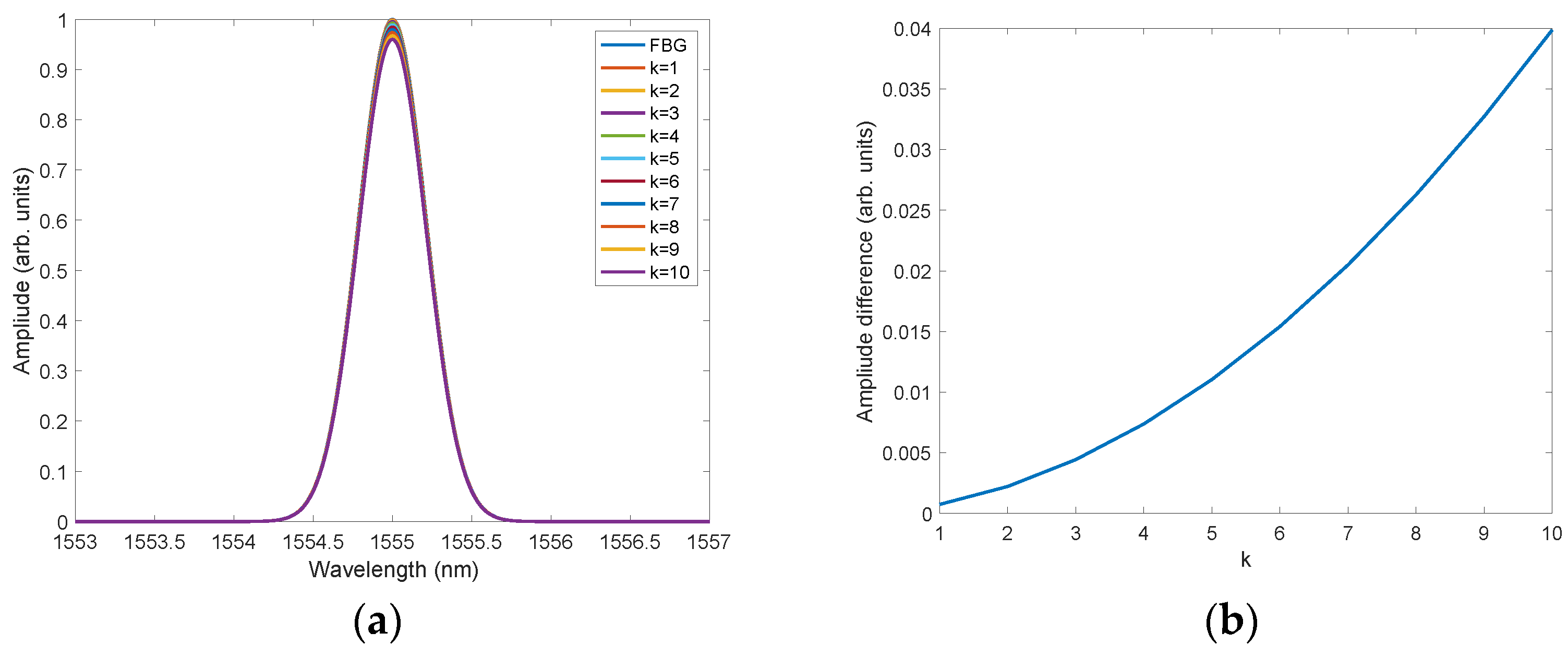
It is therefore the fifth-degree root of the product of 5 elements. Such a filter uses the current sample x[n], two previous samples x[n + 1], x[n + 2], and two subsequent samples x[n − 1] and z[n − 2] to determine the nth output value y[n]. It therefore has the properties of a noncausal filter, whose linear equivalent does not shift the output signal relative to the input signal. The effect of the Gaussian spectrum distortion by the geometric filter in Equation (3) for different values of K is shown in Figure 1. The FBG presented here has a Bragg wavelength λ_B = 1555 nm, an FWHM value of 0.5 nm, and a spectral resolution δλ = 0.01 nm.

A commonly used nonlinear operator is the discrete Teager–Kaiser energy operator [23]:

$$y\left[n\right]=x^2\left[n\right]-x[n-1]·x[n+1].$$

(4)

which is also used in an extended version introducing a differentiated delay between the product of shifted signal elements [24]:

$$y_k\left[n\right]=x^2\left[n\right]-x\left[n-k\right]·x\left[n+k\right].$$

(5)

By changing the above nonlinear differential equation from subtraction to summation, we obtain the sum of the two components. The first component is the square of the current sample value, and the second is the product of the previous and next sample values. The calculated sum should still be normalised by dividing it by two and then calculating the square root of the result. Finally, the basic version of the new filtering algorithm for the difference k = 1 is as follows:

$$y\left[n\right]={\left(\left(x^2\left[n\right]+x[n-1]·x[n+1]\right)/2\right)}^{1/2}.$$

(6)

In the version with different k delay values, the equation is

$$y_k\left[n\right]={\left(\left(x^2\left[n\right]+x[n-k]·x[n+k]\right)/2\right)}^{1/2}.$$

(7)

The final version is

$$y_{kk}\left[n\right]={\left(\sum _{k=0}^K\left(x[n-k]·x[n+k]\right)/K\right)}^{1/2}.$$

(8)

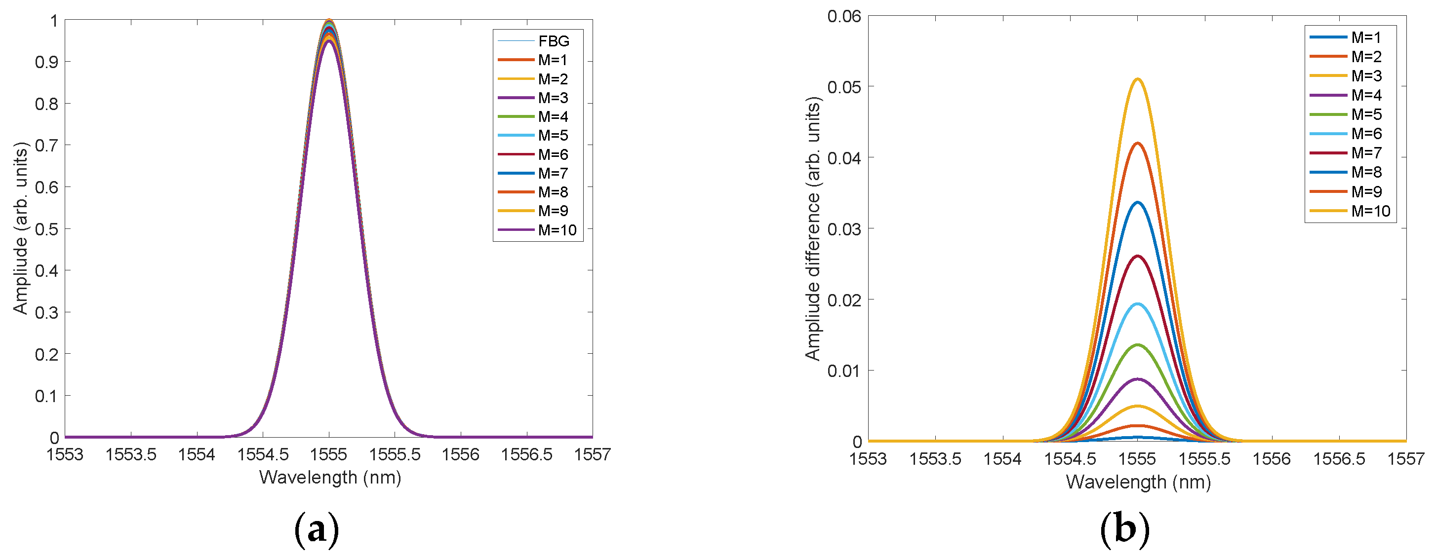
Equation (8) can be described as a symmetrical geometric–arithmetic mean filtering method. The effect of FBG spectrum distortion depending on the degree of filtration is shown in Figure 2 for the filter in the version in Equation (7). As the filter order increases, the signal intensity decreases. The difference between the original and transformed spectrum is symmetrical. Figure 3 shows the difference between the original spectrum and the spectrum after applying the filter in the version in Equation (8). A comparison of the filter’s effect on the reduction in the spectrum’s amplitude is shown in Figure 2b. The filter using the two sum components distorts the amplitude to a greater extent than the filter using the sum of K components. This property can be explained by the fact that individual products for samples farther away from the currently considered one have a greater difference in value from the central product (the value of the current input sample raised to the second power). We use the term symmetric filters due to the possibility of another asymmetric modification derived directly from the alternative version of the energy operator being called the high-order differential energy operator [25]:

$$y_k\left[n\right]=x\left[n\right]x\left[n+k-2\right]-x\left[n-1\right]·x\left[n+k-1\right],$$

(9)

which, for a third-order operator, takes the following form:

$$y_3\left[n\right]=x\left[n\right]x\left[n+1\right]-x[n-1]·x[n+2].$$

(10)

Transforming Equation (9) into filter form, we have the following notation:

$$y\left[n\right]={\left(\left(x\left[n\right]x[n+1]+x[n-1]·x[n+2]\right)/2\right)}^{1/2}.$$

(11)

The general form depending on the shift parameter k is

$$y_k\left[n\right]={\left(\left(x\left[n\right]x[n+1]+x[n-k]·x[n+k+1]\right)/2\right)}^{1/2}.$$

(12)

And, the final version of the geometric–arithmetic mean filter is

$$y_{kk}\left[n\right]={\left({\sum }_{k=0}^K\left(x[n-k]·x[n+k+1]\right)/K\right)}^{1/2}.$$

(13)

which, for K = 2, can be expressed as follows:

$$y_{22}\left[n\right]={\left(\left(x\left[n\right]x\left[n+1\right]+x\left[n-1\right]·x\left[n+2\right]+x[n-2]·x[n+3]\right)/2\right)}^{1/2}.$$

(14)

The expressions in Formulas (12) and (13) can be described as asymmetric versions of symmetric Formulas (7) and (8).

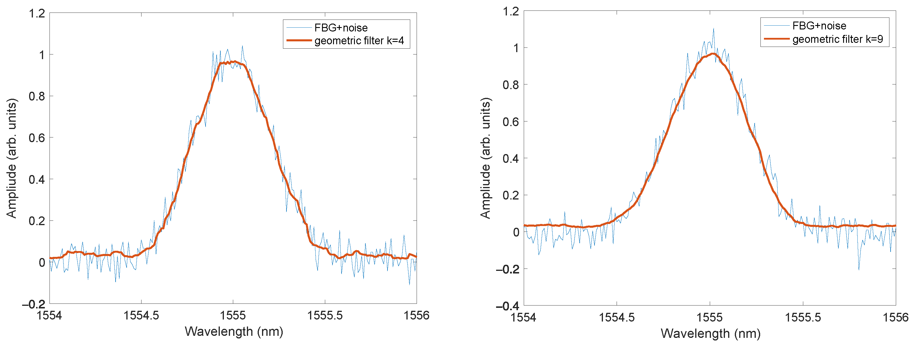
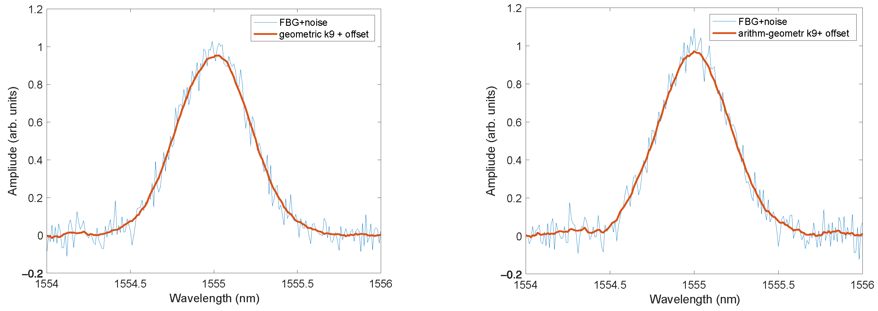
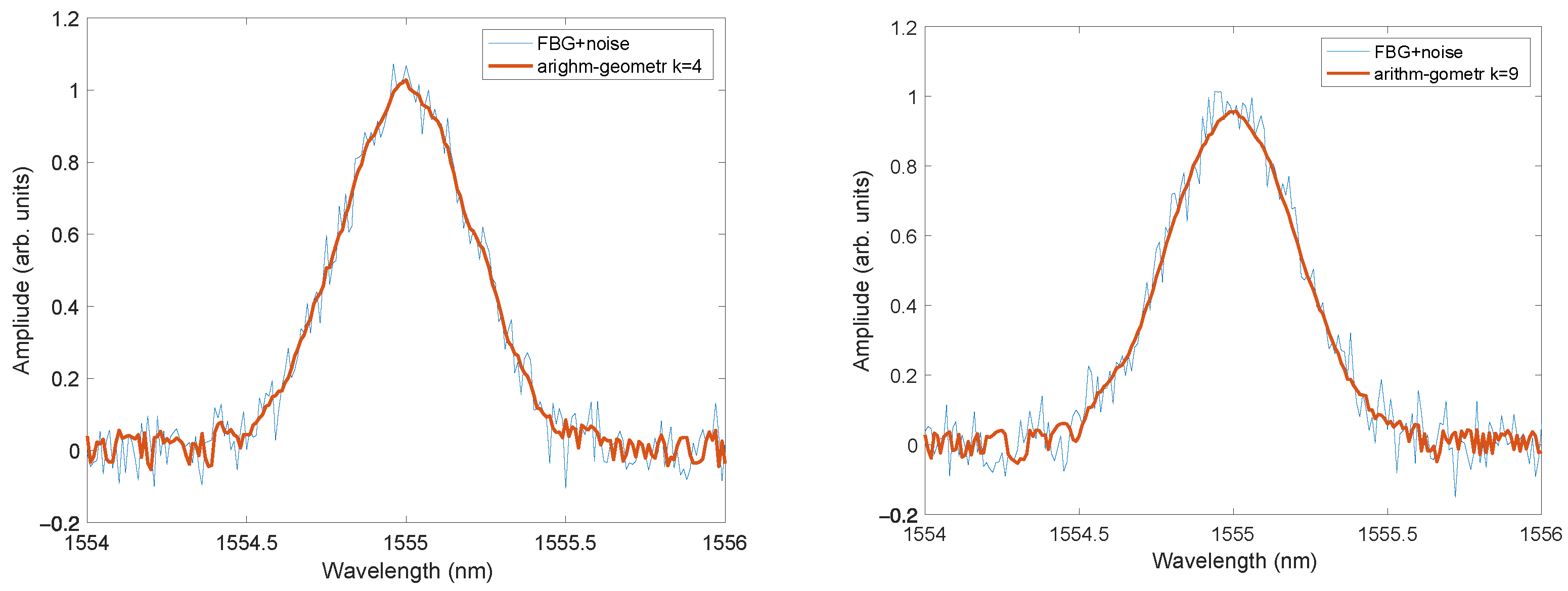
Figure 4, Figure 5, Figure 6, Figure 7, Figure 8 and Figure 9 show sample spectra with noise and spectra after nonlinear filtration. Figure 4 shows spectra with noise subjected to geometric filtering according to Formula (2) for K = 4 and K = 9. Noise with an SNR of 25 dB was added to the original spectra. Figure 5 shows the operation of the combination of mean arithmetic and mean geometric filtering according to Formula (8).

In Figure 4 and Figure 5, one can see that the performance of both nonlinear filters was worse for small signal values. In order to reduce this negative effect, a constant value (offset) was added to the spectra before filtering. After processing the spectrum by the filter, the offset was subtracted. The positive effect of such a relatively simple operation is shown in Figure 6. The benefits of offset can be seen especially when comparing Figure 6 with Figure 4 and Figure 5. During the numerical analyses, different offset values from 0.1 to 100 were tested. A positive effect occurred for all values for which the optical spectrum ceased to have negative values. Finally, we used an offset value of 1.

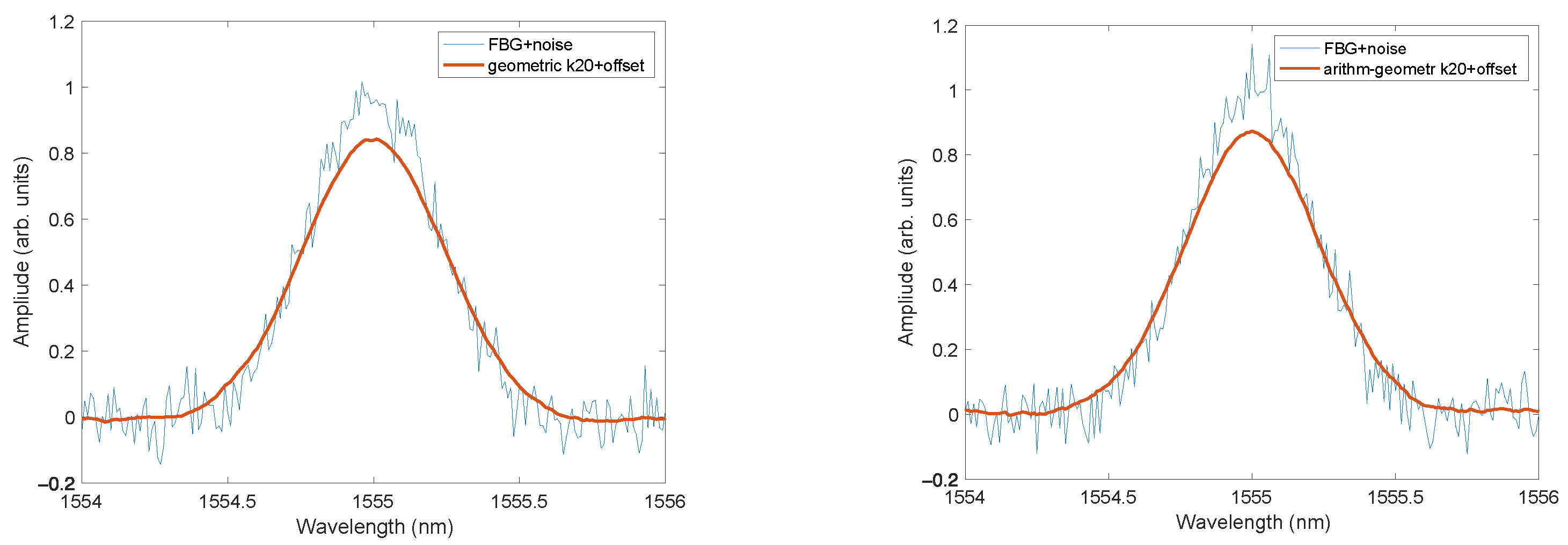
Figure 7 shows spectra subjected to nonlinear filtering with a significant value of K = 20. This is the equivalent of an impulse response length of 41 for the linear filter. The processed spectrum is devoid of visible noise features. The spectrum peak is reduced, and the half-width is increased. The effect of such processing can therefore be described as oversmoothing.

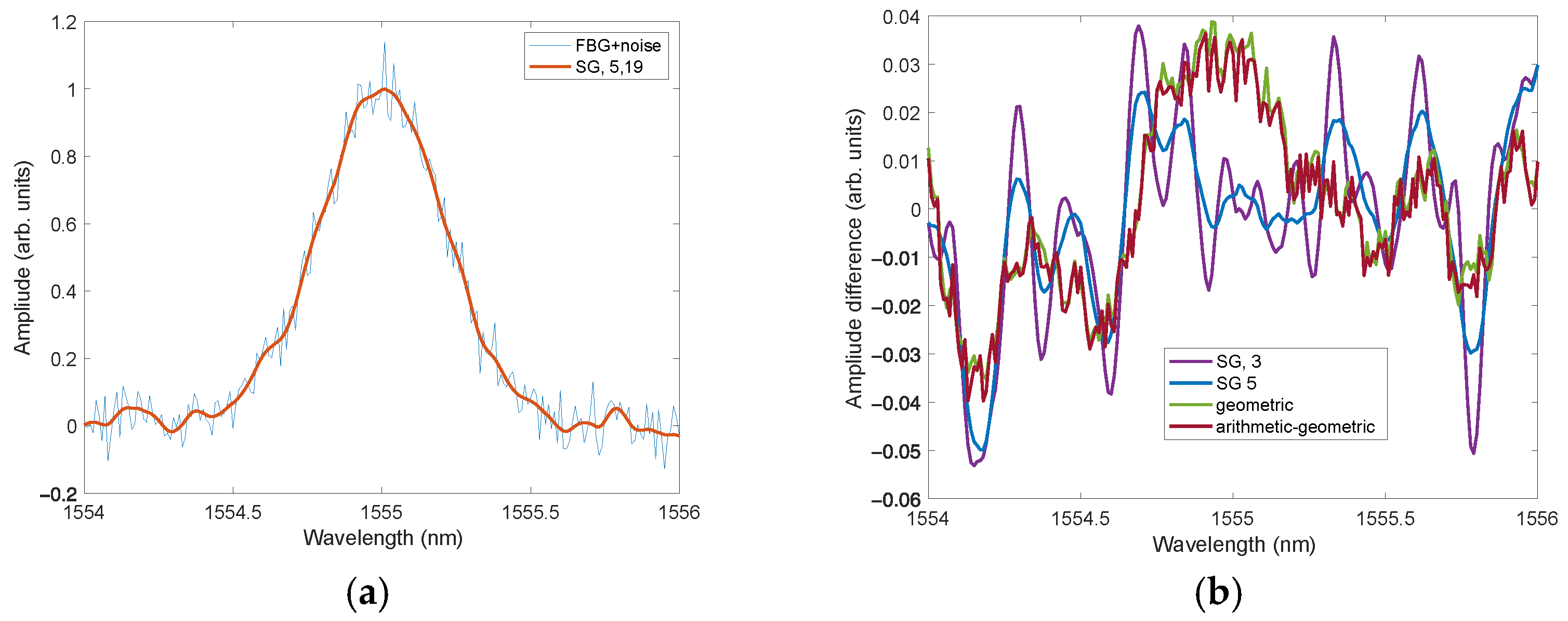
Figure 8a shows the effect of the Savitzky–Golay (SG) filter with an impulse response length of 19 and a degree of polynomial approximation of 5. Figure 8b shows the differences between the spectra after the filtering operation and without noise. Four types of filters were compared: two SG filters, geometric mean and arithmetic–geometric mean filters. The differences were smaller for nonlinear filters, especially for small amplitudes.

The computational complexity of nonlinear arithmetic–geometric filters is similar to that of finite impulse response filters implemented with convolution. For the same order of K, the same numbers of products and summations are required. In the case of a geometric filter, it is possible to reduce the number of products when calculating each output sample. An equivalent recursive filter can be used by multiplying the result by the next input sample after moving the window and dividing by the sample that has just left the window.

3. Peak Enhancement Methods

One of the actions taken to improve the resolution of determining the wavelength shift is peak shape enhancement. Due to the fact that the shape of the FBG spectrum is distorted, methods such as [13] are proposed here: derivative correction and spectrum sharpening. The use of derivatives is a well-known technique for increasing the resolution of the spectrum in spectroscopy. For FBG spectra, methods for correcting the asymmetry of the spectra have been proposed by adding their first derivative to the original spectra. The value of the weight of the correction term is determined in an iterative process [13]. Spectrum sharpening can be performed by adding and subtracting derivatives of even order [26]. Raising the Gaussian shape to power p increases the signal-to-noise ratio and reduces the half-width. Raising the signal x[n] to power p > 1 can be written as follows:

$$y\left[n\right]={\left(x\left[n\right]\right)}^p.$$

(15)

which, for a Gaussian spectrum, results in the following shape change [27]:

$$R\left(\lambda \right)=R_0^{p}exp\left(-4ln2{\left({\displaystyle \frac{\lambda -{\lambda }_B}{\left(\frac{∆{\lambda }_B}{\sqrt{p}}\right)}}\right)}^2\right),$$

(16)

so the half-width is reduced by a factor of $\sqrt{p}$.

In the case of chromatography, this allows for the separation of closely located peaks and an improvement in the signal-to-noise ratio [27]. Additionally, raising to the second power improves the peak symmetry and significantly reduces the baseline noise [28]. Raising the signal to the power is also used for time windows, which therefore have a property known as maximum sidelobe decay [29,30]. The mathematical operation of raising the signal to an even power can be used to sharpen a spectrum previously broadened by excessive smoothing. This method of combining algorithms produces an additional noise suppression effect.

4. Analysis of Spectral Shift Demodulation Methods for Simulation Data

The centroid method is used as the simplest demodulation method, which determines the equivalent of the centre of gravity of spectrum $R\left(\lambda \right)$:

$${\lambda }_B={\displaystyle \frac{\sum _n{\lambda }_B·R\left({\lambda }_n\right)}{\sum _{n}R\left({\lambda }_n\right)}}.$$

(17)

The centroid is most often calculated for wavelengths for which the reflectivity value exceeds a specified value relative to the maximum value. For a symmetric spectrum, the centre of gravity coincides with the maximum value of the spectrum. For asymmetric spectra, the centre of gravity differs from the Bragg wavelength and the maximum value of the reflectivity of the spectrum. As a demodulation method for comparing the properties of denoising methods, the cross-correlation algorithm is used, which has good properties and is also resistant to distortions of the grating spectrum [31]. The cross-correlation function between two spectra R0 and R1 can be determined as follows:

$$C_j=\sum _{i=0}^{N-1}{R}_0\left({\lambda }_i\right)R_1\left({\lambda }_{i+j}\right),$$

(18)

for j = 0, 1, 2, …, (2N − 1). Cross-correlation can be efficiently calculated in the Fourier transform domain [32]. The analysis of the cross-correlation function can be performed using the centroid algorithm or by calculating the Hilbert transform [3]. The second important method of determining the shift is the fast phase correlation (FPC) method, which consists of determining the phase difference in the Fourier transform domain between the transform of the considered spectrum F1 = FFT(R₁) and the transform of the reference spectrum F₀ = FFT(R₀). For individual frequencies, the spectral shift can be determined as follows:

$$∆{\lambda }_k=\left({\angle }_{k}FFT\left(R1\right)-{\angle }_{k}FFT\left(R0\right)\right)·{\displaystyle \frac{N·\delta \lambda }{2\pi k}}.$$

(19)

where k = 1, 2, …, (N − 1), because, for k = 0, we are dealing with a constant component, which always has a real value. The final value of the wavelength shift is the median of the shifts determined for the first dozen (several dozen) frequencies K [4]:

$$∆\lambda =median\left(∆{\lambda }_1,\dots ,∆{\lambda }_k,\dots ,∆{\lambda }_K\right)$$

(20)

The Bragg grating spectrum can be obtained based on the parameters of its structure recorded in the fibre core [33]. For a Bragg grating with applied apodisation, the reflection spectrum can be presented in the form of a Gaussian shape:

$$R\left(\lambda \right)=R_{0}exp\left(-4ln2{\left({\displaystyle \frac{\lambda -{\lambda }_B}{∆{\lambda }_B}}\right)}^2\right),$$

(21)

where $R_0$ is the peak amplitude and $∆{\lambda }_B$ is its full width at half -maximum. Real spectra may have various deviations from the ideal symmetric Gaussian shape. Additionally, the grating may undergo various deformations, for example, as a result of its nonuniform stress. The asymmetric shape of the spectrum is modelled by combining two parts of symmetric gratings [31]. The model of the asymmetric Gaussian shape is as follows [34]:

$$RR\left(\lambda \right)=\left\{\begin{array}{c}{R}_{0}exp\left(-4ln2{\left({\displaystyle \frac{\lambda -{\lambda }_B}{∆{\lambda }_B}}\right)}^2\right),\lambda <{\lambda }_B\\ R_{0}exp\left(-4ln2{\left({\displaystyle \frac{\lambda -{\lambda }_B}{\chi ·∆{\lambda }_B}}\right)}^2\right),\lambda \ge {\lambda }_B\end{array}\right.,$$

(22)

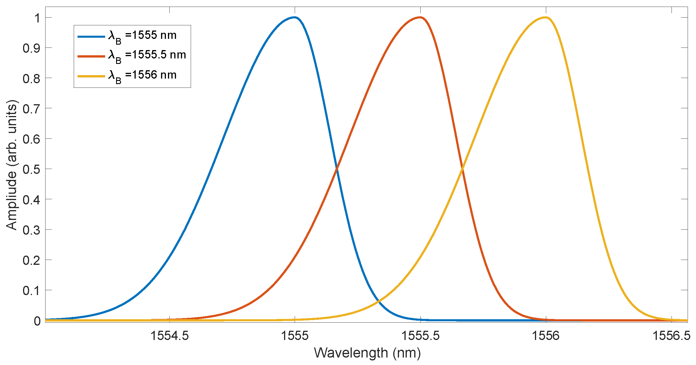
where the parameter χ is used to determine the degree of spectral asymmetry. Asymmetric spectra with an FWHM value of 0.5 nm and an asymmetry parameter value of χ = 2 were selected for simulation and numerical analysis of demodulation algorithms (Figure 9). The Bragg wavelength was changed in the range of 1 nm for 1001 values. The spectra were calculated assuming a spectral resolution of 0.01 nm. In the next step, noise with seven SNR values in the range from 30 to 60 dB was added to the spectra.

Figure 9. Example of FBG spectra with three wavelength shift values.

Figure 9. Example of FBG spectra with three wavelength shift values.

The root mean square error (RMSE) determined for M wavelength shifts of the simulated spectrum was used to evaluate the algorithms and methods of spectrum filtering and enhancement:

$$RMSE=\sqrt{{\displaystyle \frac{\sum _{m=1}^M{\left(∆{\lambda }_t\left(m\right)-∆{\lambda }_e\left(m\right)\right)}^2}{M}}},$$

(23)

where $∆{\lambda }_t$ is the real value of the spectral shift, and $∆{\lambda }_e$ is the wavelength shift calculated with the specified algorithm and preprocessing method.

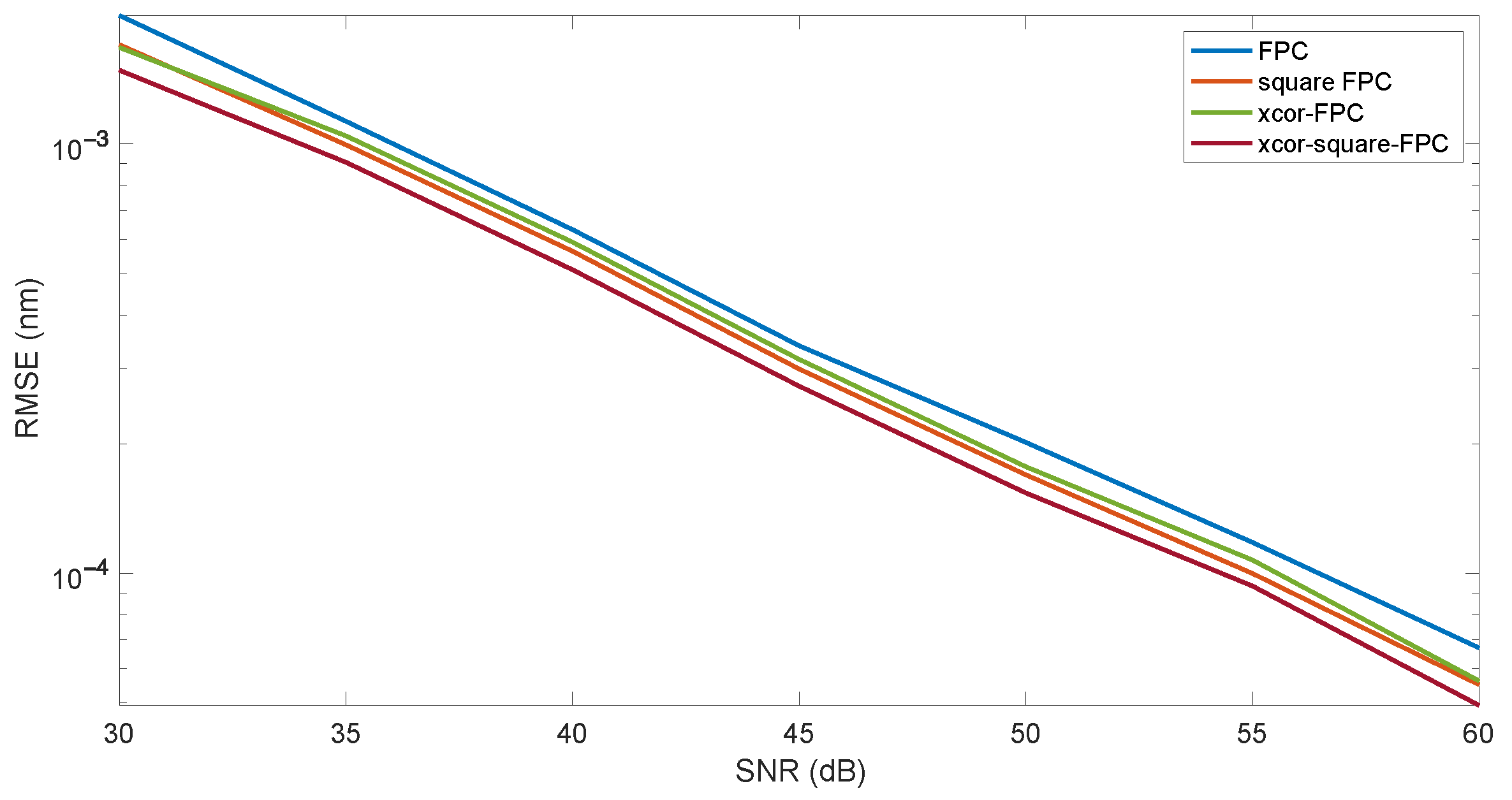
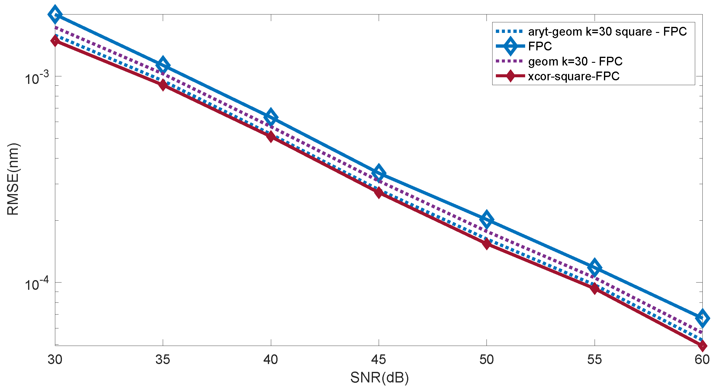
Figure 10 presents the characteristics of the dependence of the RMSE value on the SNR value for the FCP method and its modifications. The modifications consist of the initial processing of the spectrum by raising its value to the second power. The second proposed modification is the calculation of the FPC for the cross-correlation function. However, the most effective is the calculation of the shift using the FPC for the cross-correlation function raised to the second power (Figure 10).

In the analysis of various types of measurement data, preliminary smoothing is often used. For data containing shapes in the form of various types of peaks, such as spectra in spectroscopy, Savitzky–Golay (SG) filters [35] cope very well with the smoothing task. They can perform filtration with the simultaneous lack or slight distortion of the spectrum, manifested as a decrease in the intensity of the peaks. The effect of using SG filters is shown in Figure 11. With the appropriate selection of the degree of the approximating polynomial, the effect of filtration is comparable to the application of the cross-correlation function before calculating the FPC. The calculations were performed for polynomial degrees from one to seven and different lengths of the filter impulse response. The most beneficial was the use of filters with a small approximating polynomial degree. This means significant smoothing and blurring (broadening) of the spectrum. Figure 11 shows graphs for two sample filters for which the filtration effect was the most beneficial. After filtering, the individual spectrum values should be raised to the second power.

Numerical analysis was then performed on the spectra that were filtered nonlinearly using both geometric mean filters and the developed combination of mean arithmetic and geometric filters. Figure 12 presents the effect of nonlinear filtration on demodulation. Greater benefits were obtained using the combined arithmetic–geometric method. It was possible to obtain an RMSE level comparable to the use of preliminary cross-correlation. This effect was obtained for a filter operating range K = 30, which was equivalent to an impulse response length of the linear filter of 60. In each case, after filtering, the spectrum value should be raised to the second power.

The selection of the filter impulse response length, as in the case of any smoothing filtering, is made on the basis of multiple trials. Often, the result of smoothing filtering is assessed in terms of its visual effect. In the case of FBG spectra, the filter response length depends on the spectral resolution of the measurement and the half-width of the grid. For linear filters, the filter is selected through frequency analysis and cut-off frequency. For nonlinear filters, concepts such as the frequency response or transmittance cannot be used. Therefore, specific input data sequences must be analysed, and, based on them, conclusions about the filtration properties can be drawn. For the analysed spectra, we were interested in the effect of filters on reducing the RMSE of wavelength demodulation methods. Therefore, the visual effects of filtration presented in Figure 1, Figure 2, Figure 3, Figure 4, Figure 5, Figure 6, Figure 7 and Figure 8 do not necessarily translate directly into an improvement in the quality of spectra demodulation. The cross-correlation method itself is a method that reduces noise. The fast phase correlation method is also relatively resistant to the noise content of data. The combination of these two methods seems to be optimal in terms of the robustness of the demodulation methods to noise. Replacing cross-correlation with a filter provides an equally useful demodulation method. During the numerical calculations, we also checked the possibilities of raising the spectrum to a power higher than two. However, it turned out that, for p = 3 and p = 4, the RMSE results were not as good as for p = 2. The method of raising to the second power and then filtering is also a less advantageous solution than filtering before raising to the second power. 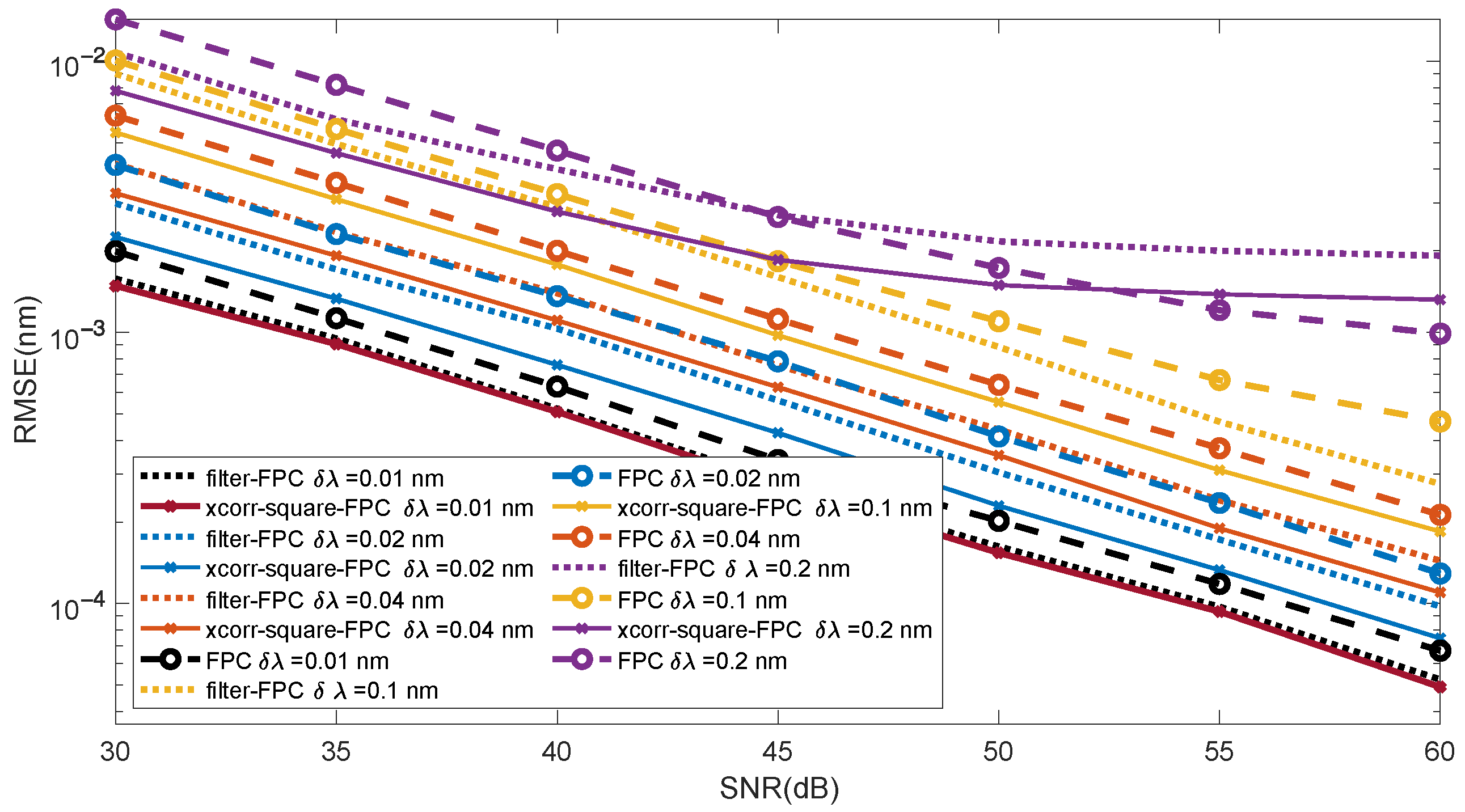Figure 13 shows a comparison of the effect of the spectral resolution on the RMSE of three algorithms. The spectral resolutions analysed were δλ = 0.01, 0.02, 0.04, 0.1, and 0.2 nm. The worst results were achieved for the directly applied FPC method. Both the application of geometric–arithmetic filters and the initial cross-correlation reduced the RMSE values. However, slightly better results were obtained using cross-correlation.

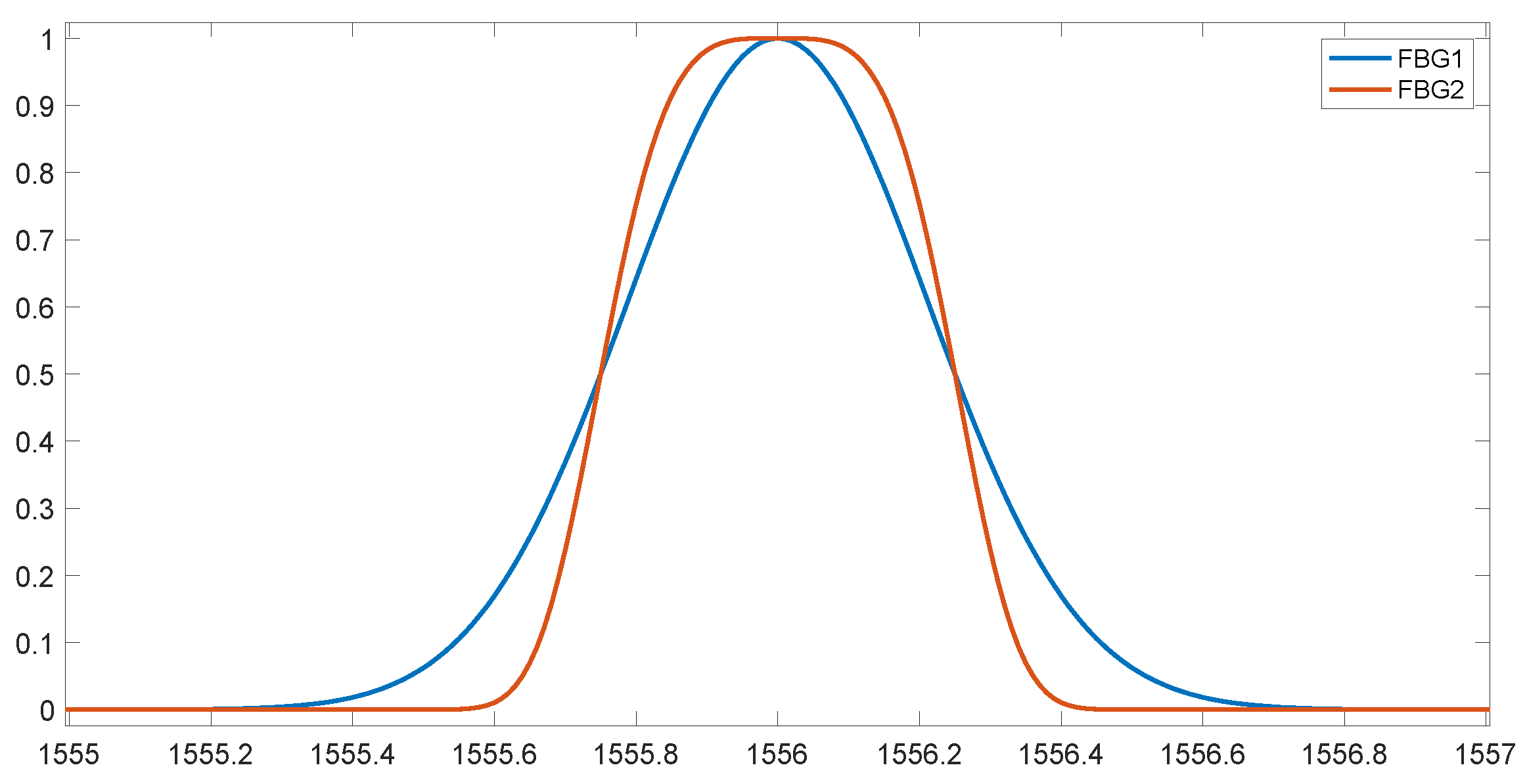
The next simulations consisted of using the two types of grating spectra shown in Figure 14. The FWHM value of both gratings was 0.5 nm. The FBG1 had a Gaussian shape, while the FBG2 had a characteristic spectrum with a flat-top shape. Such a spectrum was obtained as a result of using the fourth-order Gaussian function. As for the previous simulations, the spectral resolution was 0.01 nm. The simulations used 1001 values of the Bragg wavelength shift in the 1 nm range.

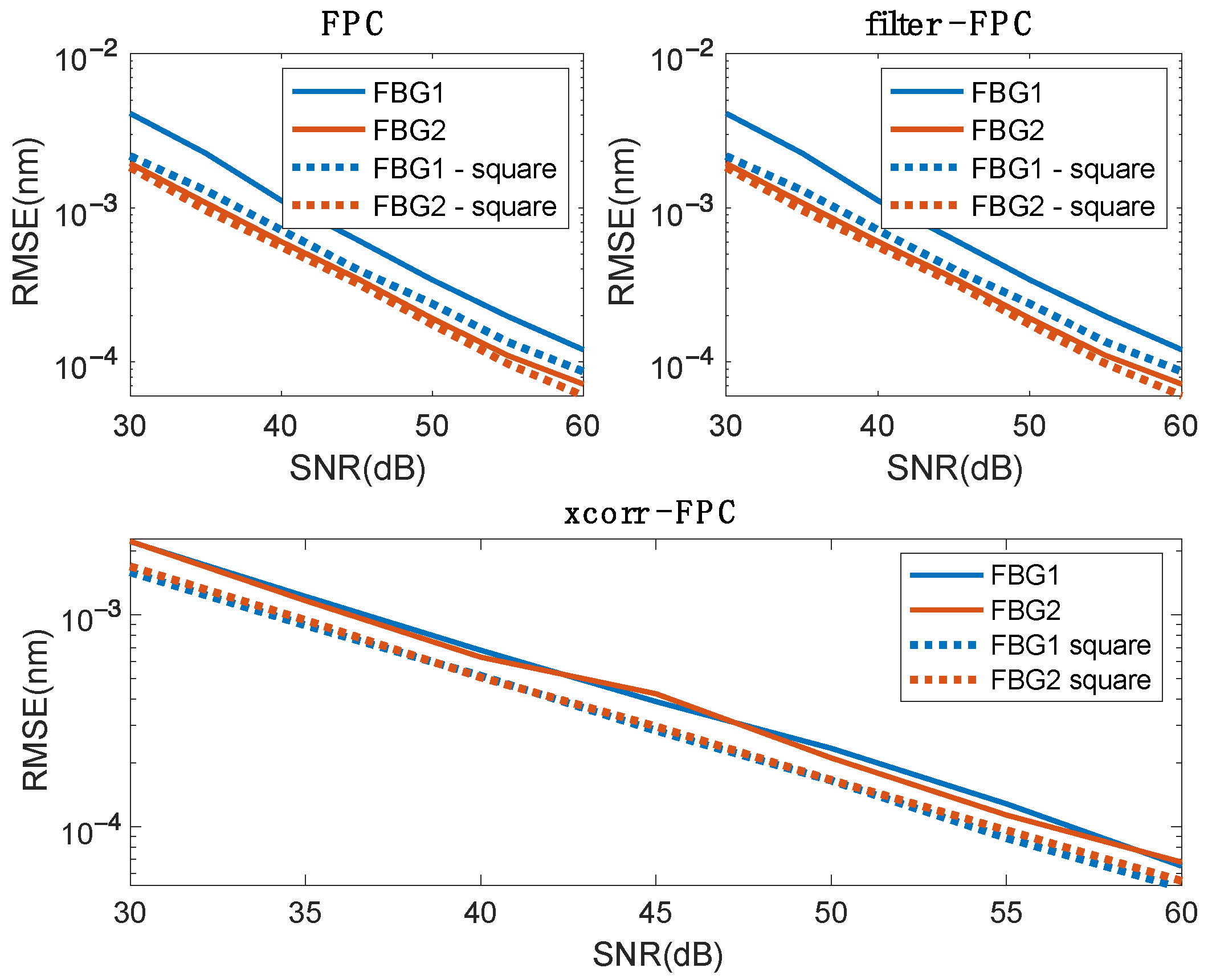
Figure 15 shows a comparison of RMSE values for two gratings from Figure 14. In order to better compare the influence of the type of spectrum, individual algorithms are presented in separate parts of the figure. The analysed algorithms were the direct FPC method, FPC preceded by an arithmetic–geometric filter, and FPC preceded by cross-correlation. For the FPC algorithm, direct analysis of the spectrum and the spectrum raised to the second power was performed. Raising to the power was noticeably beneficial for FBG1. For FBG2, the RMSE improvement was small. Similar results were obtained for the use of filtration before calculating the FPC. For both direct FPC methods and the filter with FPC, the FBG2 was characterised by lower RMSE values. In the case of the cross-correlation method, there were no differences between FBG1 and FBG2. For both gratings, it was beneficial to raise the calculated cross-correlation function to the second power.

5. Experimental Data Analysis

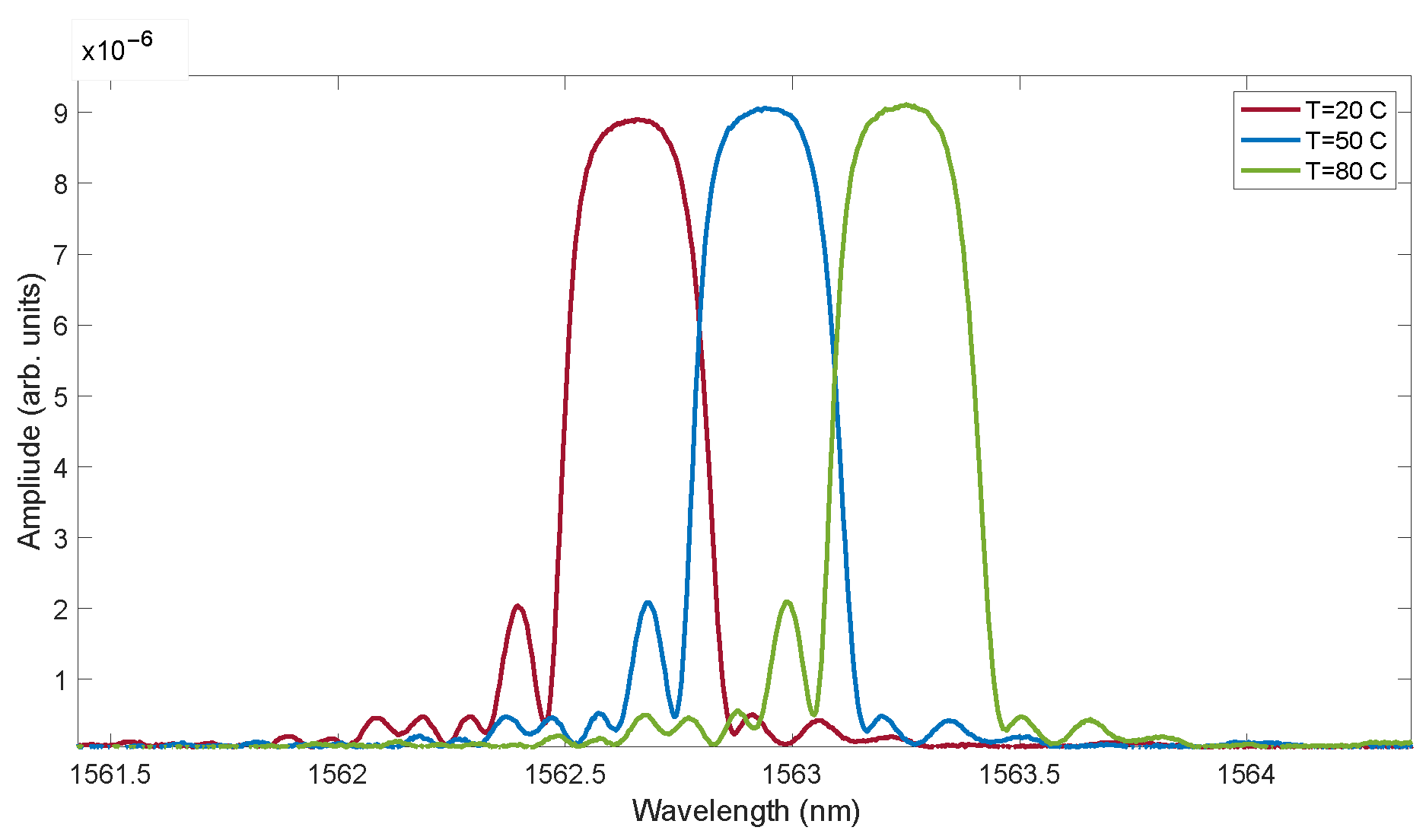
The experiment was conducted using the standard laboratory equipment shown in Figure 16. Measurements were performed in reflective mode with the following components: an optical spectrum analyser (OSA; AQ6370D, Yokogawa Electric Corporation, Kanagawa, Japan), a superluminescent diode (SLD), an optical circulator, and a fibre Bragg grating (FBG) used as a temperature sensor. The light emitted from the SLD source was transmitted through an optical fibre to the first port of the optical circulator and subsequently directed to the second port, which was connected to the FBG sensor placed inside a temperature chamber. The reflection spectra were measured using the OSA, with a resolution of 0.004 nm, connected to the third port of the circulator. Examples of spectra measured at a fixed temperature are presented in Figure 17.

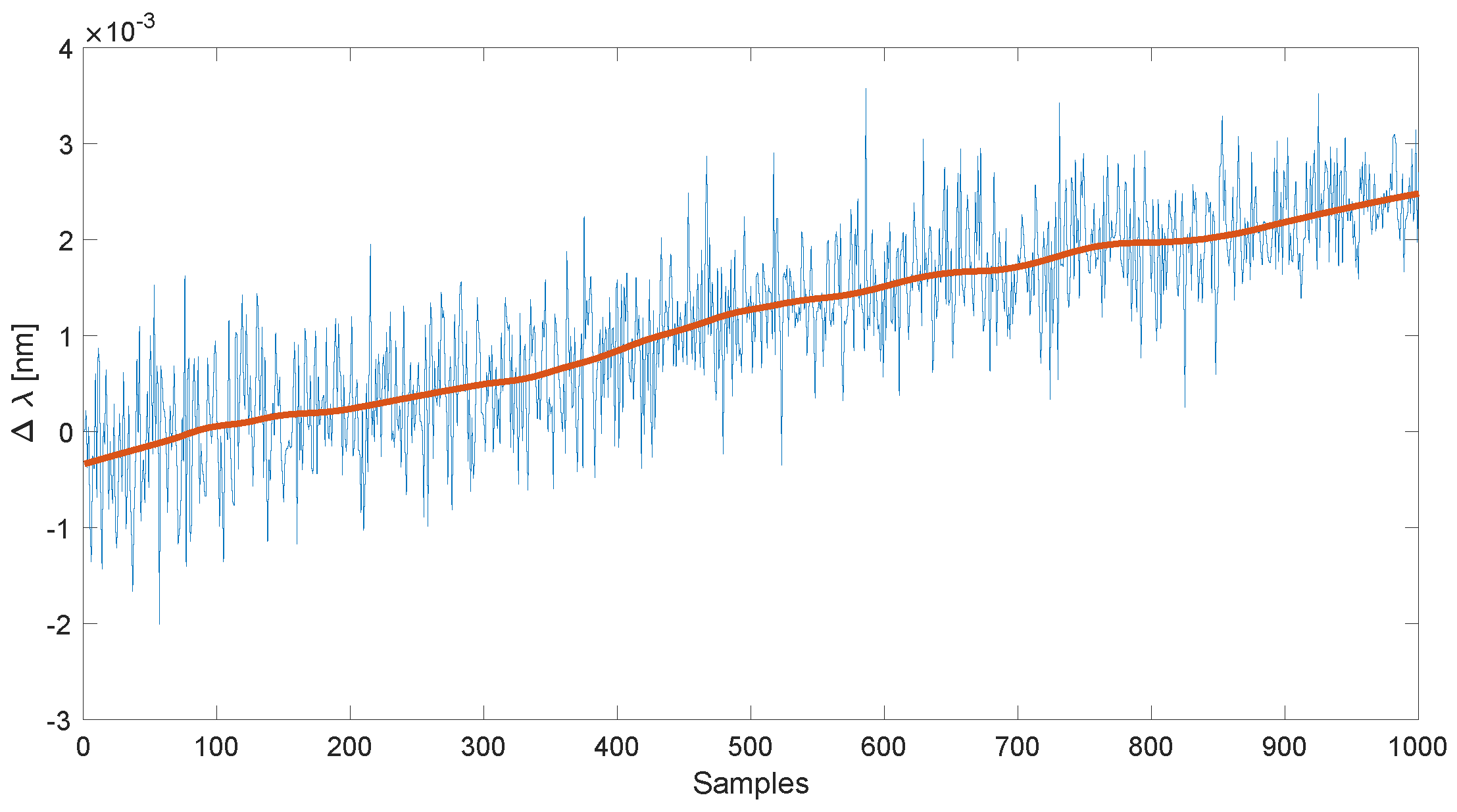
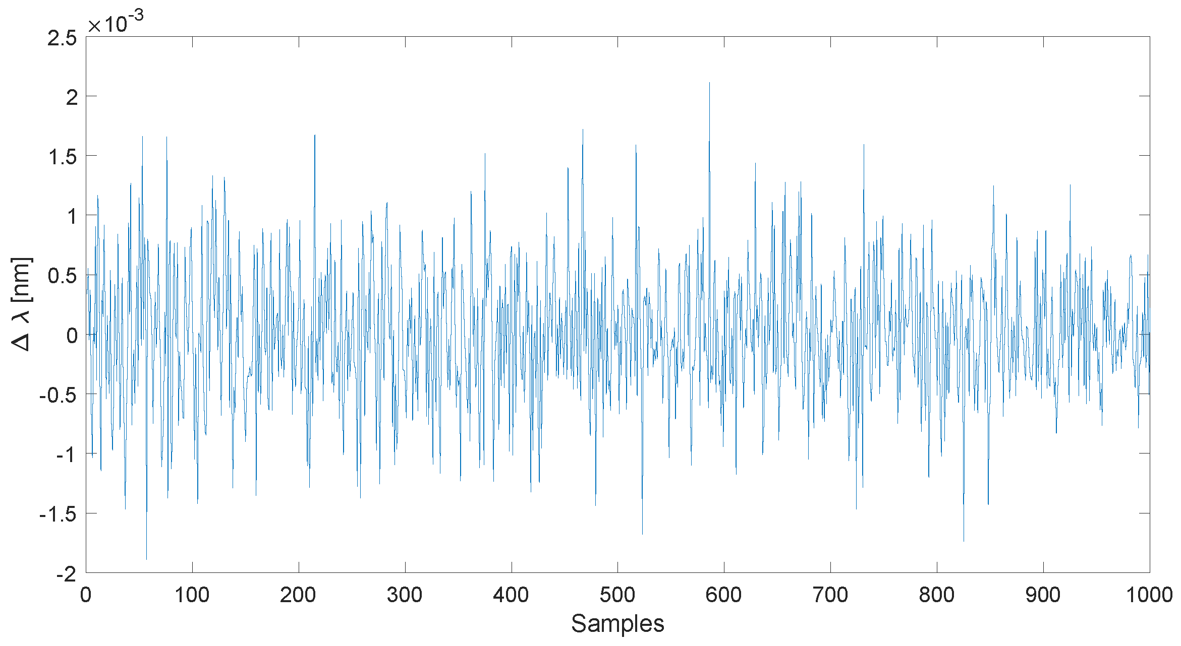
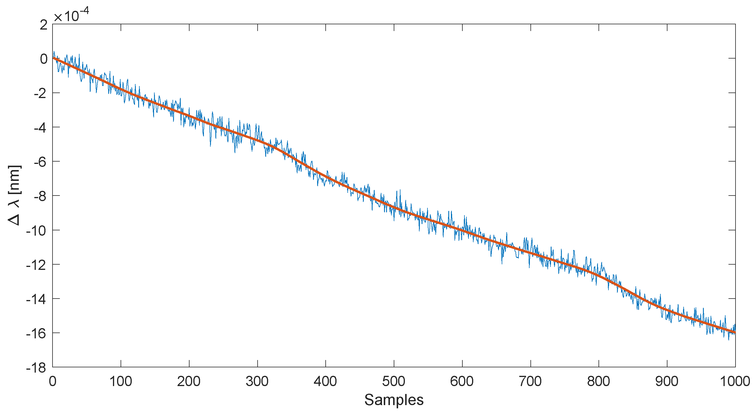
Details regarding the first part of the experiment are presented in Appendix A. Measurements were performed for three values of the steady-state temperature and during the heating process. Due to the significant visible fluctuations in the determined wavelength during the heating process, additional experiments were performed. This time, the temperature in the climatic chamber was set to 20 °C, which was identical to the ambient temperature. Then, a temperature stabilisation system, which included, amongst others, a mechanical fan, was turned off. The course of the changes in the spectrum shift length as a function of the sample number is presented in Figure 18. Individual spectra were measured every 3 s. The shift was determined using the centroid algorithm, where the spectrum values were previously raised to the second power. 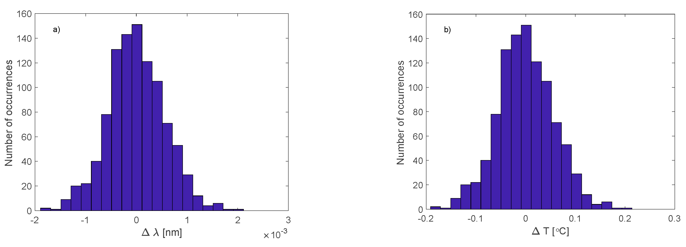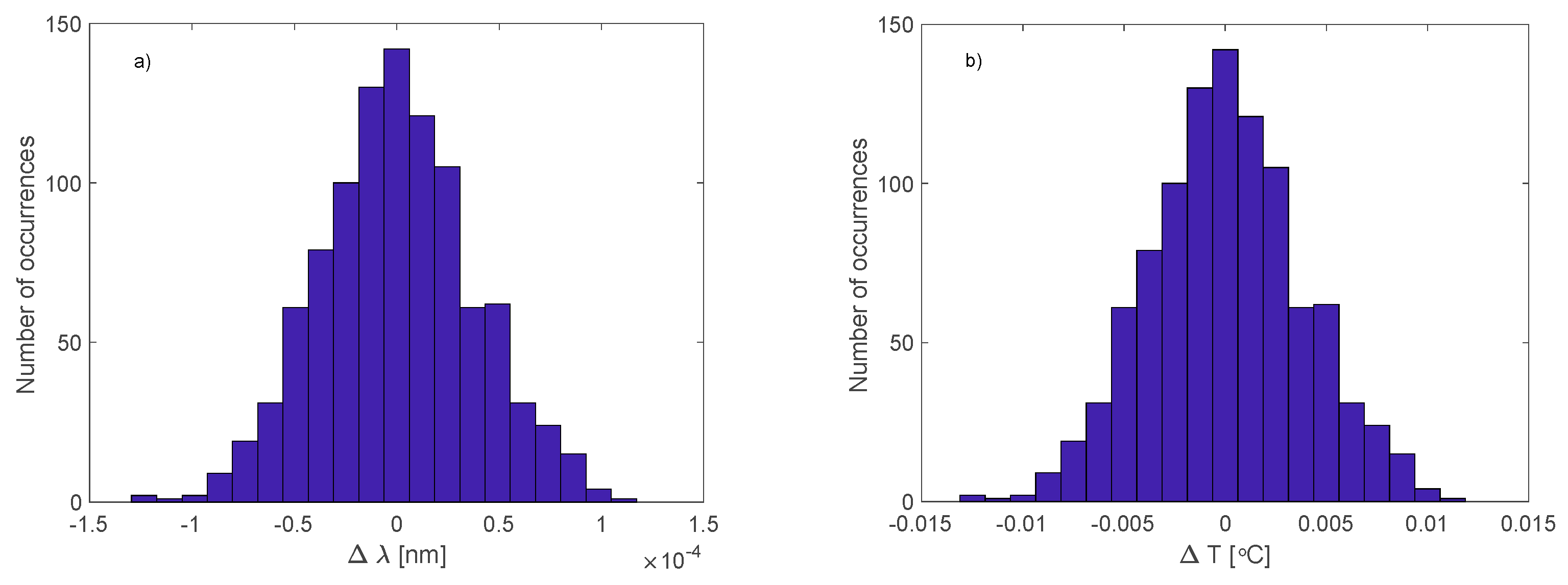The standard deviation of measurements without a trend was 0.37 × 10⁻⁴ nm. At a sensitivity of 9.87 pm/°C, this corresponded to a standard deviation of the determined temperature of 0.0038 °C. Histograms of the error distribution are presented in Figure 19. Similar to the previous measurements, the distributions of values deviating from the trend line were close to the normal distribution. The trend component decreased during the measurements by 1.6 pm, which meant a temperature decrease of 0.16 °C. The trend line was determined using local regression for 15% of the length of the analysed signal. A linear function was used as the regression function.

Table 1. Comparison of the standard deviation of the measurement for individual algorithms. Spectral resolution $\delta \lambda$ = 0.004 nm.

Algorithm	$\mathbf{STD}\mathit{\lambda }$ (pm)	STD T (°C)
Centroid	0.4199	0.0425
Power of spectrum–centroid	0.0374	0.0038
FPC	0.0420	0.0043
Power of spectrum–FPC	0.0398	0.0040
Nonlinear filter (k = 40)–FPC	0.0369	0.0037
Cross-correlation–FPC	0.0403	0.0041
Cross-correlation–square–FPC	0.0381	0.0039

presents a comparison of the standard deviation of the wavelength changes (STD λ) calculated for several demodulation algorithms. In each case, raising the spectrum to the second power caused a decrease in the standard deviation value. The most favourable change occurred for the centroid algorithm, because the standard deviation decreased more than tenfold. The use of a nonlinear filter with significant smoothing (K = 40) before the FPC algorithm was equivalent to a positive effect on the calculation of cross-correlation.

In

Table 2. Comparison of the standard deviation of the measurement for individual algorithms. Spectral resolution $\delta \lambda$ = 0.02 nm.

Algorithm	$\mathbf{STD}\mathit{\lambda }$ (pm)	STD T (°C)
Centroid	0.882	0.0894
Power of spectrum–centroid	0.068	0.0069
FPC	0.184	0.0186
Power of spectrum–FPC	0.142	0.0144
Nonlinear filter (k = 8)–FPC	0.076	0.0077
Cross-correlation–FPC	0.079	0.0080
Cross-correlation–square–FPC	0.069	0.0070

, we present the results of the analysis of demodulation methods when changing the spectral resolution of the measured spectra. In each measurement spectrum, every fifth sample was selected, which corresponded to a change in the spectral resolution from 0.004 nm to 0.02 nm. For spectra with a smaller number of points, the STD values were obviously higher. However, the effect of filtering and raising the spectrum to the second power was more significant.

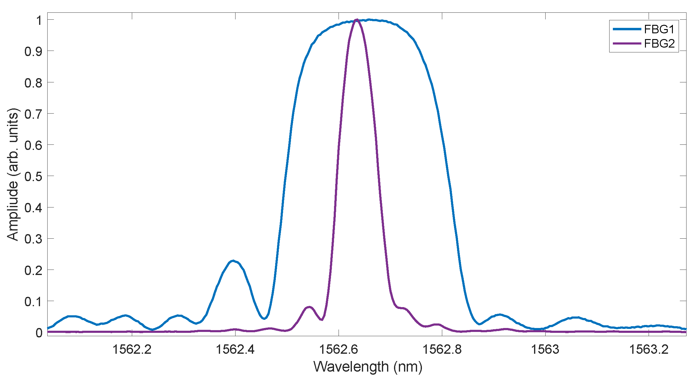
In order to confirm the agreement of the obtained results for gratings with other parameters, further measurements were carried out at a temperature of 20 °C. The second FBG2 had a shape more similar to Gaussian compared to the first FBG1, which had a wider spectrum with a flat-top shape (Figure 20).

Similar to the temperature measurements for the first FBG1 grid, 1000 measurements were recorded with the temperature set at 20 °C. The numerical analysis was performed in the same way as for FBG1. A comparison of the algorithms is presented in

Table 3. Comparison of RMSE for individual algorithms and two spectral resolutions, $\delta \lambda$= 0.004 nm and $\delta \lambda$= 0.02 nm.

Algorithm	$\mathit{\delta }\mathit{\lambda }$ = 0.004 nm	$\mathit{\delta }\mathit{\lambda }$ = 0.02 nm
Centroid	0.0506	0.501
Power of spectrum–centroid	0.0405	0.412
FPC	0.0401	0.410
Power of spectrum–FPC	0.0407	0.409
Nonlinear filter (k = 40)–FPC	0.0409	0.410
Cross-correlation–FPC	0.0407	0.082
Cross-correlation–square–FPC	0.0405	0.081

. Table 3 presents only the standard deviation for the wavelength when considering two spectral resolutions, δλ = 0.004 nm and δλ = 0.02 nm.

6. Conclusions

Due to the presence of noise, the interpretation of various measurements requires the use of signal processing algorithms. Also, for measurements of FBG sensor spectra, various algorithms have been developed to estimate the Bragg wavelength and its shift. This article presents methods that reduce the noise in the measurement data for demodulation of the Bragg wave shift. The first group of methods includes nonlinear filtration, while the second is the operation of raising the spectrum value to the second power. Algorithms based on geometric filtration and its modifications reproduce the Gaussian shape well. A weaker level of noise elimination can be observed for small intensity values. A method of reducing this phenomenon, which is proposed in this article, is adding a specific offset value to the spectrum before applying the filter and subtracting this value after the filtration operation. The second method is using combined arithmetic and geometric filtration operations. This nonlinear filter has better properties than a geometric filter. With simulation data, it was found that raising the spectrum to the second power reduced the RMSE value of the shift determination for the entire considered SNR range. Before raising the spectrum to the power, it is beneficial to perform cross-correlation or, equivalently, smoothing filtration. However, unlike in the case of typical spectrum analysis, the basic condition is not preserving the peak intensity but significantly blurring it. Thanks to this, the signal-to-noise ratio in the spectrum significantly increases after filtration and raising to the second power. The analysis of the experimental spectra revealed the influence of the climatic chamber operation on the vibrations, which were noticeable in the measurements, especially in the phase of changing the temperature settings. Measurements with the temperature stabilisation function switched off significantly reduced the fluctuations of the determined wavelength compared to stabilisation during operation. The beneficial influence of the use of nonlinear filtration and raising the spectrum to the second power was also demonstrated in the case of experimental measurements.