
Determination of Length Correction from the Projection and Deformation of Geodetic Controls in the Realization of Precision Linear Structures—A Case Study of the Coordinate System S-JTSK, Czech Republic


Abstract
Featured Application
Abstract
1. Introduction
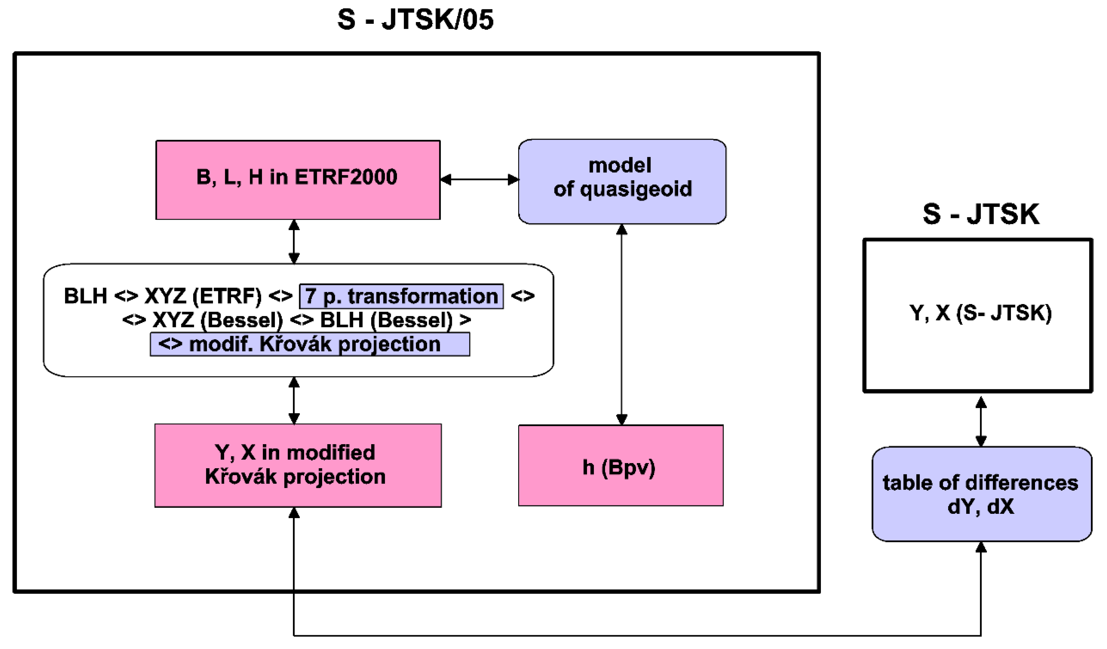
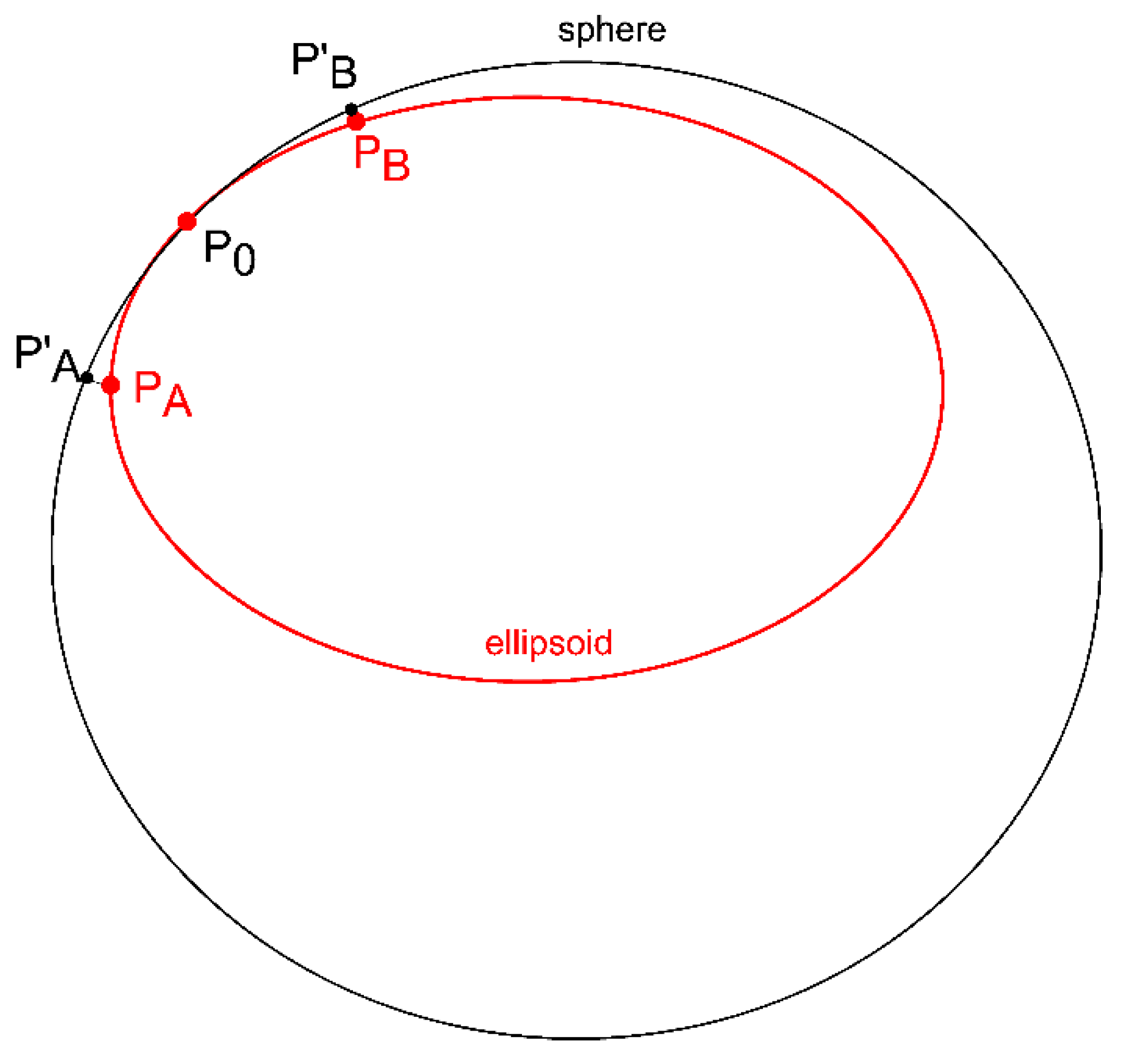
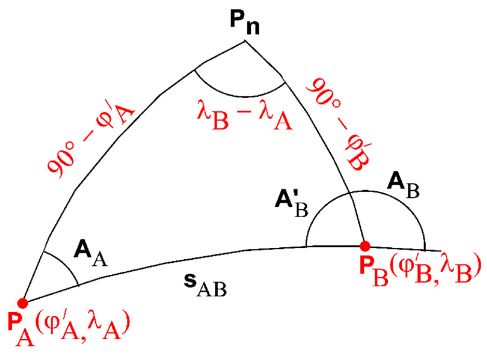
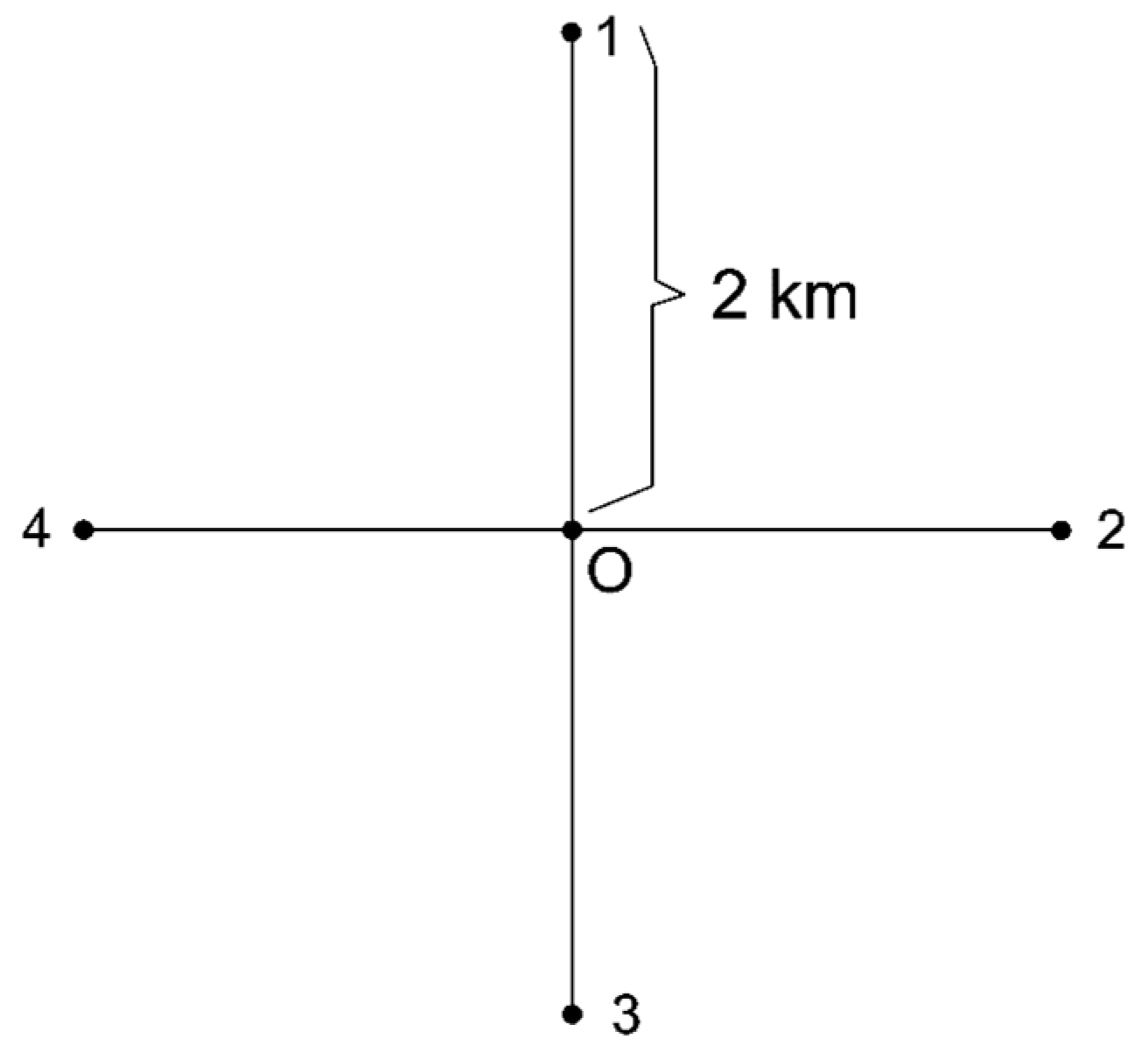
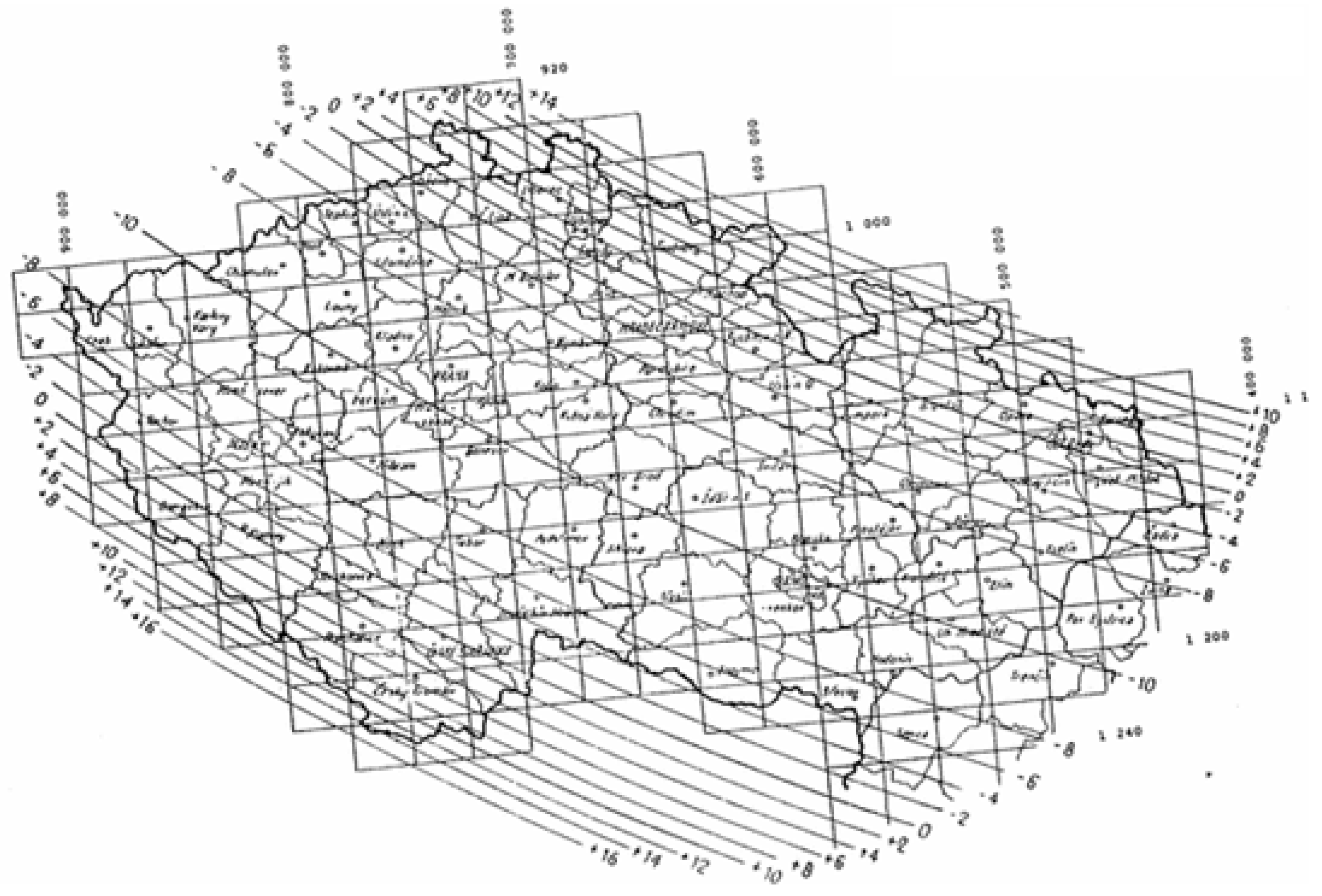
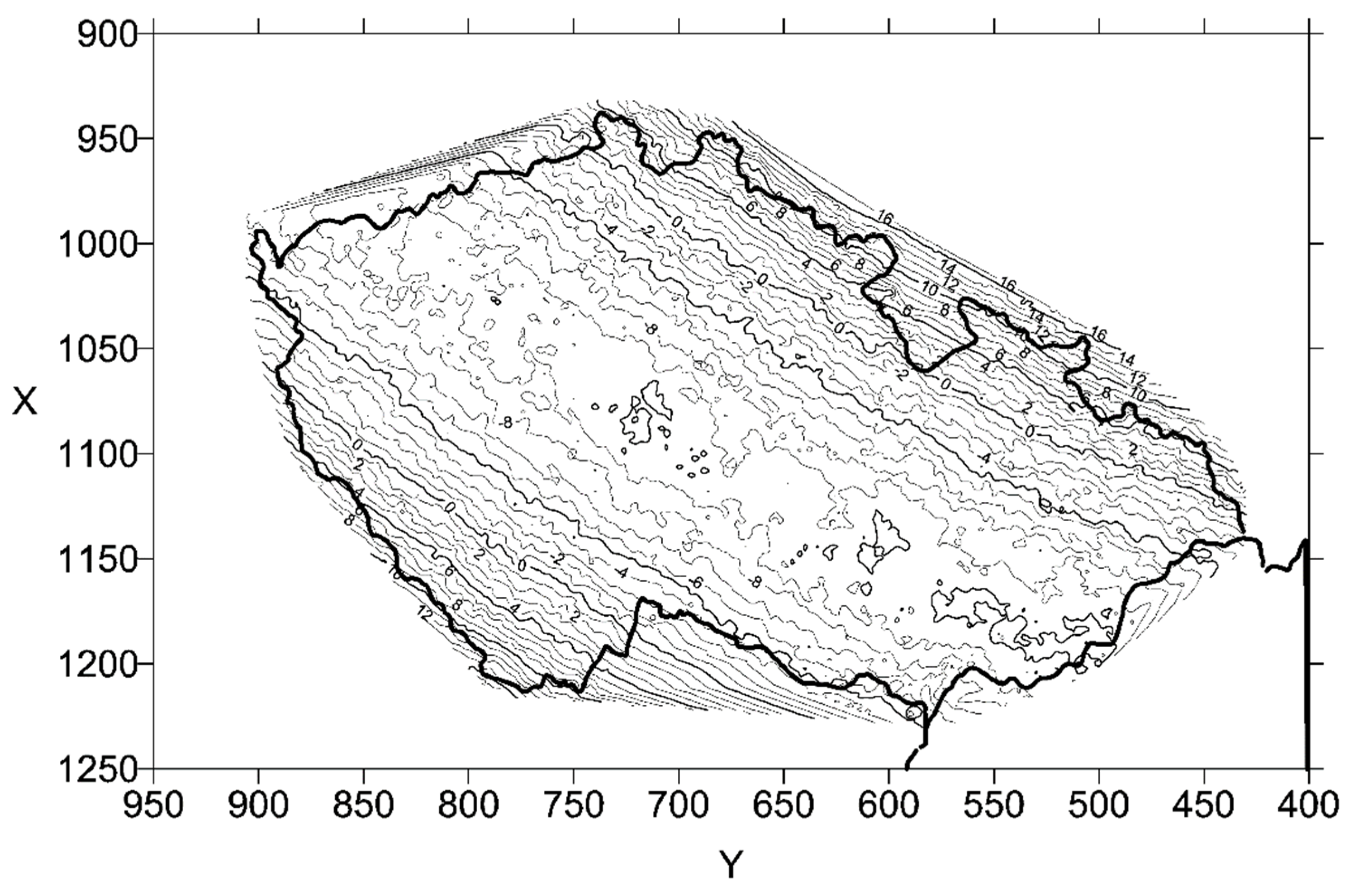
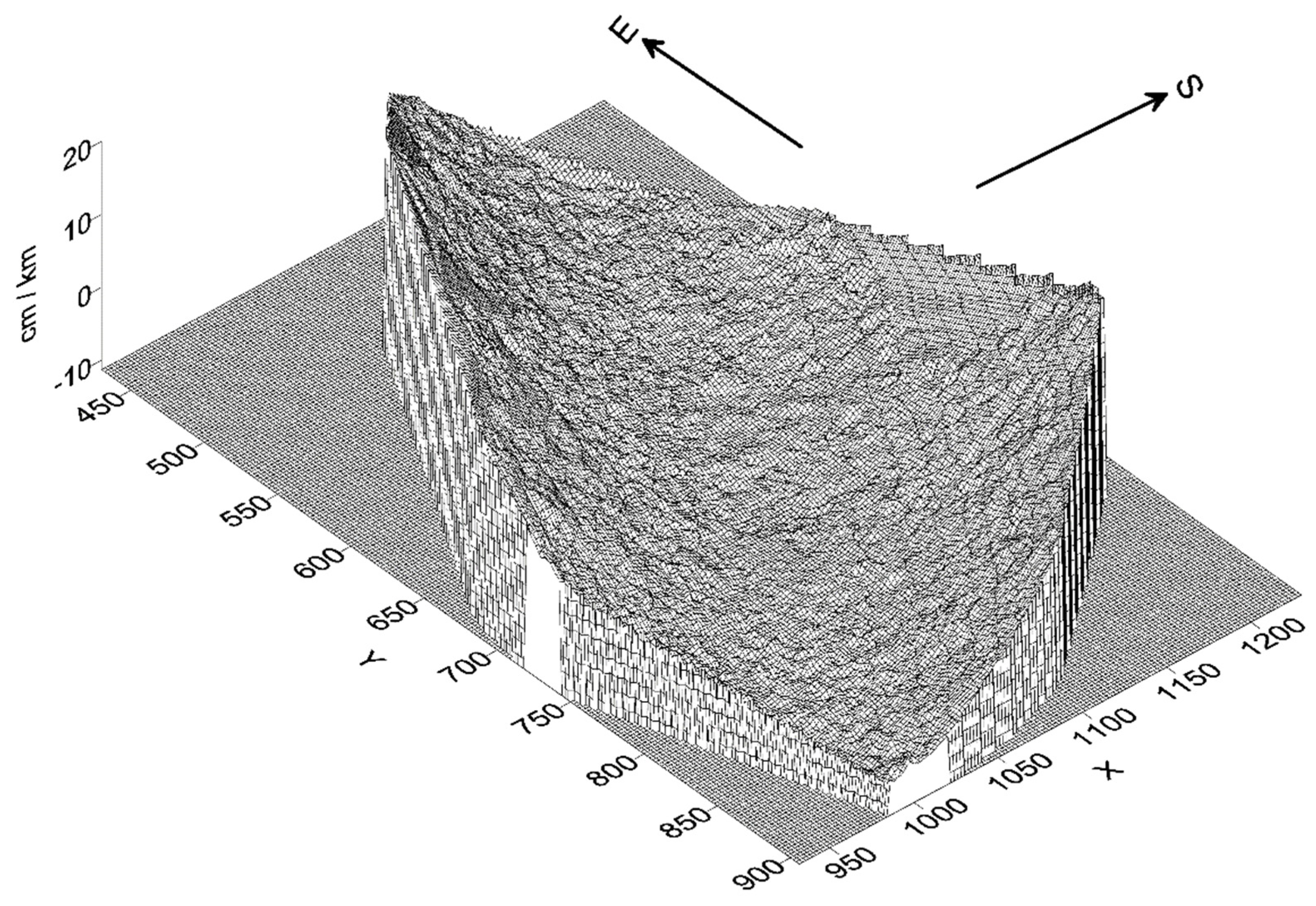
2. Calculation of the Length Correction from the Projection and Deformation
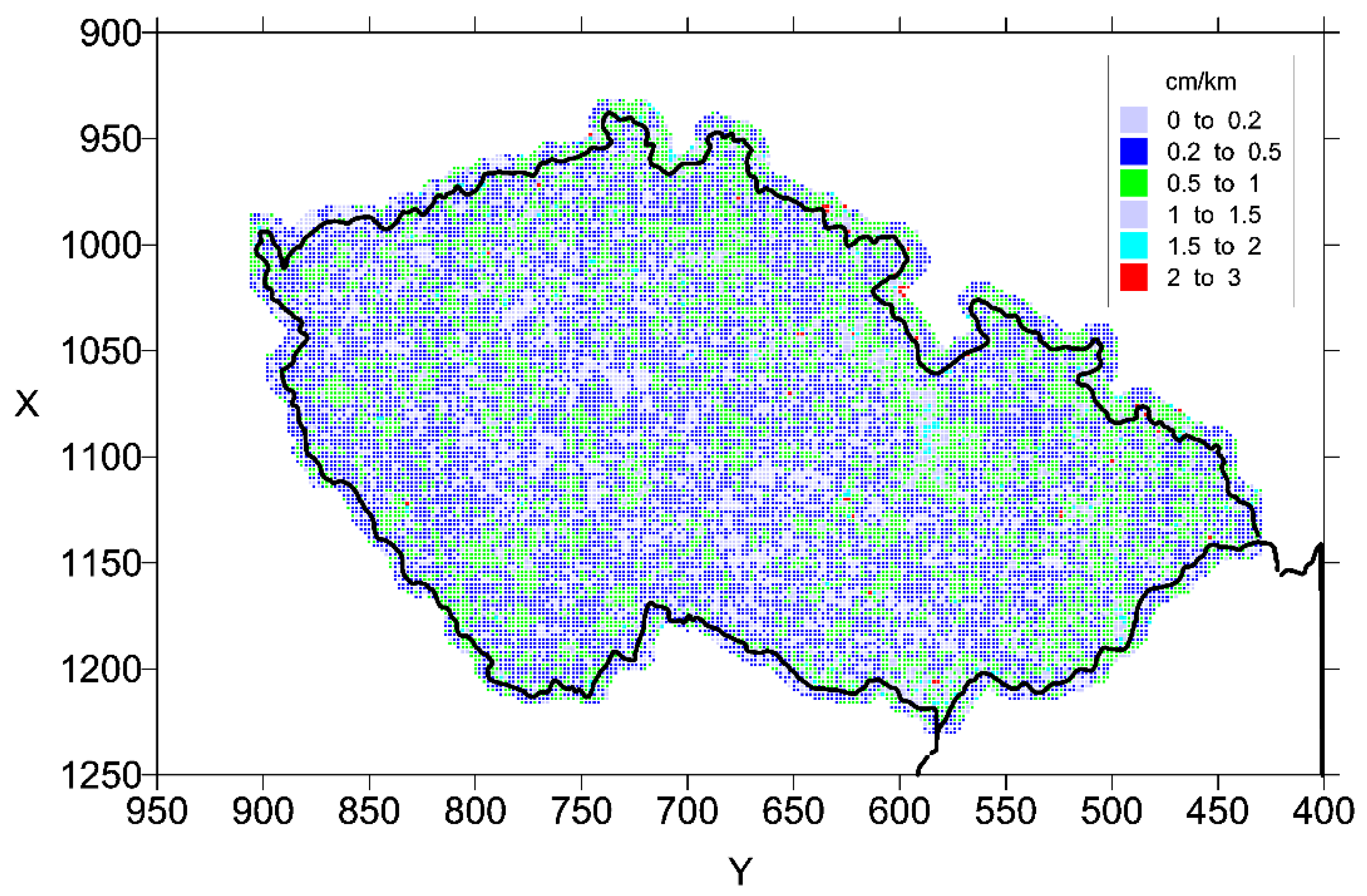
3. Results
4. Evaluation and Conclusions
Author Contributions
Funding
Institutional Review Board Statement
Informed Consent Statement
Data Availability Statement
Acknowledgments
Conflicts of Interest
Abbreviations
| CZEPOS | State network of permanent stations for localization in the Czech Republic |
| ETRF2000 | European Terrestrial Reference Frame 2000 |
| ETRS89 | European Terrestrial Reference System 1989 |
| GNSS | Global Navigation Satellite Systems |
| GRS80 | Geodetic Reference System 1980 |
| LCC | Lambert conformal conic projection |
| RTK | Real-Time Kinematic |
| S-JTSK | System of the Unified Trigonometric Cadastral Network |
| S-JTSK/05 | Working version of S-JTSK |
References
- Cada, V.; Vichrova, M. Horizontal Control for Stable Cadastre and Second Military Survey (Franziszeische Landesaufnahme) in Bohemia, Moravia and Silesia. Acta Geod. Geophys. Hung. 2009, 44, 105–114. [Google Scholar] [CrossRef]
- Berkova, A. Digitized Cadastral Map from a Point of View of Compiler from Geometric Plan. Acta Montan. Slovaca 2007, 12, 318–324. [Google Scholar]
- Cechurova, M.; Veverka, B. Cartometric Analysis of the Czechoslovak Version of 1:75 000 Scale Sheets of the Third Military Survey (1918–1956). Acta Geod. Geophys. Hung. 2009, 44, 121–130. [Google Scholar] [CrossRef]
- Gasincova, S.; Gasinec, J.; Hudeckova, L.; Cernota, P.; Stankova, H. Analysis of the Usability of the Maps from the Former Cadastre of Lands in Terms of Parcels Area Registered in the Cadastral Documentation. Inz. Miner. J. Pol. Miner. Eng. Soc. 2018, 2, 191–200. [Google Scholar]
- Berkova, A. Cadastral Map Supersession Acording New Instructions. Acta Montan. Slovaca 2009, 14, 12–18. [Google Scholar]
- Skokanova, H.; Havlicek, M. Military Topographic Maps of the Czech Republic from the First Half of the 20th Century. Acta Geod. Geophys. Hung. 2010, 45, 120–126. [Google Scholar] [CrossRef]
- Mackovcin, P.; Jurek, M. New Facts About Old Maps of the Territory of the Former Czechoslovakia. Geografie 2015, 120, 489–506. [Google Scholar] [CrossRef]
- Bartonek, D.; Bures, J.; Svabensky, O. Optimized GNSS RTK Measurement Planning for Effective Point Occupation via Heuristic Analysis. Eng. Comput. 2017, 34, 90–104. [Google Scholar] [CrossRef]
- Cernota, P.; Stankova, H.; Fecko, P.; Pospisil, J.; Bedrunka, M. Connecting and Orientation of the Horizon of Mine Workings. In Proceedings of the 11th International Multidisciplinary Scientific Geoconference (SGEM 2011), Albena, Bulgaria, 18–24 June 2011; Volume I, pp. 735–742. [Google Scholar]
- Kovanic, L. Geodetic Monitoring of the Mine Activities Impact Using GNSS Technology and Ensuring Visualization of Results in GIS. In Proceedings of the 13th International Multidisciplinary Scientific Geoconference (SGEM 2013), Geoconference on Informatics, Geoinformatics and Remote Sensing, Conference Proceedings, Albena, Bulgaria, 16–22 June 2013; Volume II, pp. 221–228. [Google Scholar]
- Veverka, B. Krovak’s Projection and Its Use for the Czech Republic and the Slovak Republic. In 50 Years of the Research Institute of Geodesy, Topography and Cartography: Jubilee Proceedings, 1951–2004; Holota, P., Ed.; Research Institute of Geodesy, Topography and Cartography Publications: Zdiby, Czech Republic, 2005; Volume 50, pp. 173–179. [Google Scholar]
- Gasinec, J.; Gassincova, S.; Trembeczka, E. Derivation of Simplified Formulas for the Approximate Calculation of the Meridian Convergence and Scale Error in Krovak Projection. Inz. Miner. J. Pol. Miner. Eng. Soc. 2014, 15, 77–84. [Google Scholar]
- Bartonek, D.; Bures, J. Usage of Heuristic Algorithm for Optimization of Precise GNSS RTK Measurement. In Proceedings of the 15th International Multidisciplinary Scientific Geoconference (SGEM), Informatics, Geoinformatics and Remote Sensing, Albena, Bulgaria, 18–24 June 2015; Volume I, (SGEM 2015). pp. 899–906. [Google Scholar]
- Nevosad, Z. To RTK points in CZEPOS Network. Acta Montan. Slovaca 2007, 12, 482–486. [Google Scholar]
- Svabensky, O.; Weigel, J. Long-term Positional Monitoring of Station VYHL of the Sneznik Network. Acta Geodyn. Geomater. 2007, 4, 201–206. [Google Scholar]
- Pospisil, L.; Svabensky, O.; Rostinsky, P.; Novakova, E.; Weigel, J. Geodynamic Risk Zone at Northern Part of the Boskovice Furrow. Acta Geodyn. Geomater. 2017, 14, 113–129. [Google Scholar] [CrossRef]
- Weiss, G.; Gasinec, J.; Zeliznakova, V.; Gasincova, S. Using the Total Least Square Method by Deformation Strain Analyses of the Eastern Edge Eastern Tatras. Inz. Miner. J. Pol. Miner. Eng. Soc. 2014, 1, 213–226. [Google Scholar]
- Al-Toobi, Y.; Al-Hashmi, S.; Al-Busaidi, B.; Al-Balushi, I.; Ses, S. Establishment of new Oman National Geodetic Datum ONGD14. Surv. Rev. 2015, 47, 418–428. [Google Scholar] [CrossRef]
- Ristic, K.; Tucikesic, S.; Milinkovic, A. Inventarization of the Benchmarks NVT II Network in the Field of the Republic of Srpska and Application of DGNSS Technology. In Advanced Technologies, Systems and Applications III; Lecture Notes in Networks and Systems; Springer: Cham, Switzerland, 2019; Volume 60, pp. 213–223. [Google Scholar] [CrossRef]
- Seidl, M.; Trasak, P. PPROJ.4 Cartographic Projection Library as 3D Transformation Tool in Czech Context. In Proceedings of the 14th International Multidisciplinary Scientific Geoconference (SGEM), Geoconference in Informatics, Geoinformatics and Remote Sensing, Albena, Bulgaria, 17 June 2014; Volume II, pp. 395–401. [Google Scholar]
- Kostelecký, J.; Cimbálník, M.; Čepek, A.; Douša, J.; Filler, V.; Kostelecký, J.; Nágl, J.; Pešek, I.; Šimek, J. Implementation of S-JTSK/05. Geod. Cartogr. Rev. 2012, 58, 145–154. Available online: https://uazk.cuzk.cz/mrimage/vademecum/proxy/cz/others/zeus/knih/dao/documents/0001/4ee053f6-83e6-46ac-8081-d257ce19e221.pdf (accessed on 2 February 2025). (In Czech).
- Kostelecký, J.; Kostelecký, J.; Pešek, I. Conversion Methodology Between ETRF2000 and S-JTSK. VÚGTK and ČVUT in Prague, July 2010. Available online: https://docplayer.cz/34890599-Metodika-prevodu-mezi-etrf2000-a-s-jtsk-varianta-2.html (accessed on 2 February 2025). (In Czech).
- Nágl, J.; Řezníček, J. Calculation of the new version of the conversion tables for the refined global transformation between the S-JTSK and ETRS89 reference systems (version 2017-10). Geod. Cartogr. Rev. 2018, 64, 213–221. Available online: https://uazk.cuzk.cz/mrimage/vademecum/proxy/cz/others/zeus/knih/dao/documents/0001/804dc8f9-8cbb-455a-bebb-06d8a6323b94.pdf (accessed on 2 February 2025). (In Czech).
- Kostelecký, J. Global Position Coordinate Systems; Czech Technical University in Prague: Prague, Czech Republic, 2019; ISBN 978-80-01-06571-6. (In Czech) [Google Scholar]
- Cimbálník, M.; Veverka, B. Czech Technical University, Faculty of Civil Engineering, Prague, Czech Republic. Personal communication, 1996. [Google Scholar]
- State Administration of Land Surveying and Cadastre. Principles for the Use of Programs etrf00-jtsk_v1012, etrf00-jtsk_v1203 and etrf00-jtsk_v1801 for the Transformation of the Results of Measurement Activities for the Needs of the Real Estate Cadastre of the Czech Republic. State Administration of Land Surveying and Cadastre. Prague. Available online: https://www.cuzk.cz/Zememerictvi/Geodeticke-zaklady-na-uzemi-CR/GNSS/etrf00-jtsk-v1012-a-etrf00-jtsk-v1203.aspx (accessed on 2 February 2025). (In Czech).
- Vincenty, T. Direct and inverse solutions of geodesics on the ellipsoid with application of nested equations. Surv. Rev. 1975, 23, 88–93. [Google Scholar] [CrossRef]
- Sjobeg, L.E.; Shirazian, M. Solving the Direct and Inverse Geodetic Problems in the Ellipsoid by Numerical Integration. J. Surv. Eng. ASCE 2012, 138, 9–16. [Google Scholar] [CrossRef]
- Panou, G.; Delikaraoglou, D.; Korakitis, R. Solving the geodesics on the ellipsoid as a boundary value problem. J. Geod. Sci. 2013, 3, 40–47. [Google Scholar] [CrossRef]
- Karney, C.F.F. Algorithms for geodesics. J. Geod. 2013, 87, 43–55. [Google Scholar] [CrossRef]
- Vykutil, J. Advanced Geodesy; Kartografie Praha: Prague, Czech Republic, 1982; 544p, ISBN 29-620-82. (In Czech) [Google Scholar]
- Pacinek, E. Relationship Between ETRS89 and S-JTSK: Determination of Length Correction from Projection and from S-JTSK Deformation. Diploma Theses, Technical University of Ostrava, Faculty of Mining and Geology, Department of Geodesy and Mining Surveying, Ostrava, Czech Republic, 2022. (In Czech). [Google Scholar]


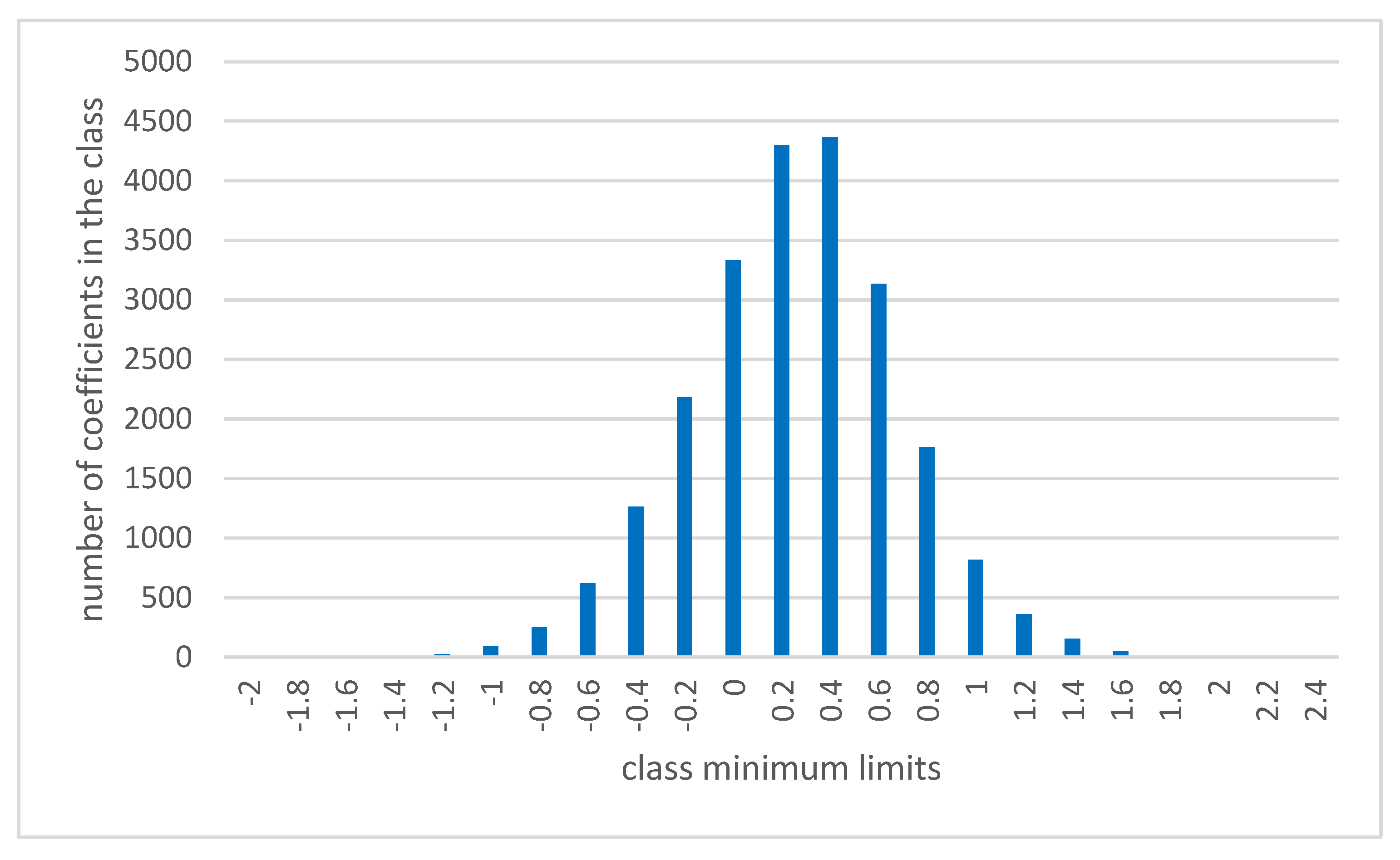
| Average | 0.36 |
| Minimum | −1.63 |
| Maximum | +2.50 |
| Interval of Classes in cm/km | Frequency of Corrections in Classes | Representation in [%] |
|---|---|---|
| <−2.0; −1.8> | 0 | 0.00 |
| <−1.8; −1.6> | 1 | 0.00 |
| <−1.6; −1.4> | 3 | 0.01 |
| <−1.4; −1.2> | 8 | 0.04 |
| <−1.2; −1.0> | 25 | 0.11 |
| <−1.0; −0.8> | 89 | 0.39 |
| <−0.8; −0.6> | 252 | 1.11 |
| <−0.6; −0.4> | 625 | 2.75 |
| <−0.4; −0.2> | 1263 | 5.55 |
| <−0.2; 0.0> | 2181 | 9.59 |
| <0.0; 0.2> | 3332 | 14.7 |
| <0.2; 0.4> | 4296 | 18.9 |
| <0.4; 0.6> | 4366 | 19.2 |
| <0.6; 0.8> | 3134 | 13.8 |
| <0.8; 1.0> | 1760 | 7.74 |
| <1.0; 1.2> | 819 | 3.60 |
| <1.2; 1.4> | 360 | 1.58 |
| <1.4; 1.6> | 155 | 0.68 |
| <1.6; 1.8> | 49 | 0.22 |
| <1.8; 2.0> | 13 | 0.06 |
| <2.0; 2.2> | 8 | 0.04 |
| <2.2; 2.4> | 1 | 0.00 |
| <2.4;2.6> | 1 | 0.00 |
| <2.6; 2.8> | 0 | 0.00 |
| <2.8; 3.0> | 0 | 0.00 |
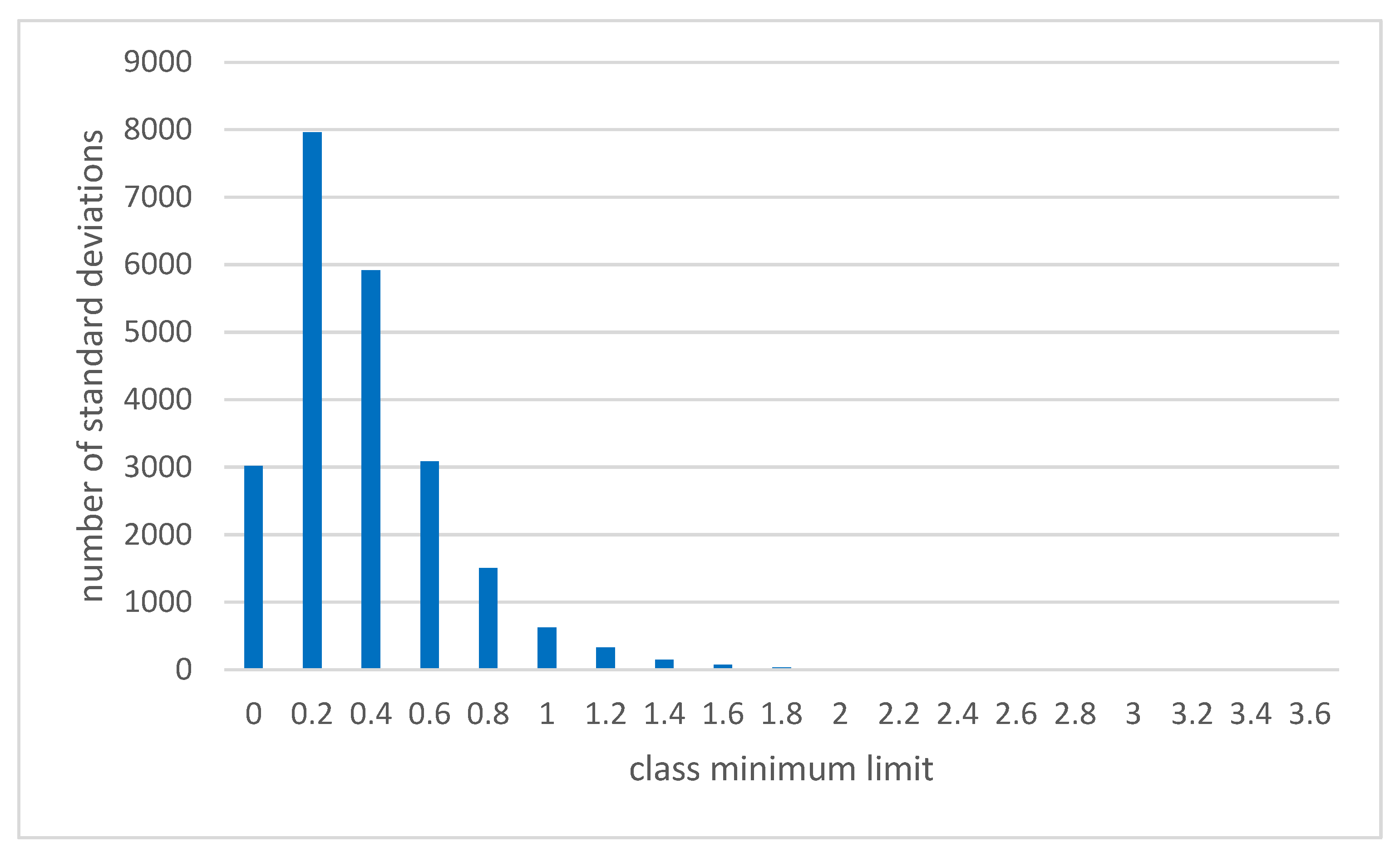
| Average | 0.47 |
| Minimum | +0.01 |
| Maximum | +3.61 |
| Interval of Classes in cm/km | Frequency of Standard Deviations in Classes | Representation in [%] |
|---|---|---|
| <0.0; 0.2> | 3017 | 13.3 |
| <0.2; 0.4> | 7960 | 35.0 |
| <0.4; 0.6> | 5916 | 26.0 |
| <0.6; 0.8> | 3089 | 13.6 |
| <0.8; 1.0> | 1506 | 6.62 |
| <1.0; 1.2> | 623 | 2.74 |
| <1.2; 1.4> | 329 | 1.45 |
| <1.4; 1.6> | 151 | 0.66 |
| <1.6; 1.8> | 76 | 0.33 |
| <1.8; 2.0> | 31 | 0.14 |
| <2.0; 2.2> | 21 | 0.09 |
| <2.2; 2.4> | 10 | 0.04 |
| <2.4; 2.6> | 6 | 0.03 |
| <2.6; 2.8> | 2 | 0.01 |
| <2.8; 3.0> | 2 | 0.01 |
| <3.0; 3.2> | 1 | 0.00 |
| <3.2; 3.4> | 0 | 0.00 |
| <3.4; 3.6> | 0 | 0.00 |
| <3.6; 3.8> | 1 | 0.00 |
Disclaimer/Publisher’s Note: The statements, opinions and data contained in all publications are solely those of the individual author(s) and contributor(s) and not of MDPI and/or the editor(s). MDPI and/or the editor(s) disclaim responsibility for any injury to people or property resulting from any ideas, methods, instructions or products referred to in the content. |
© 2025 by the authors. Licensee MDPI, Basel, Switzerland. This article is an open access article distributed under the terms and conditions of the Creative Commons Attribution (CC BY) license (https://creativecommons.org/licenses/by/4.0/).
Share and Cite
Kostelecky, J.; Cernota, P.; Stankova, H. Determination of Length Correction from the Projection and Deformation of Geodetic Controls in the Realization of Precision Linear Structures—A Case Study of the Coordinate System S-JTSK, Czech Republic. Appl. Sci. 2025, 15, 3369. https://doi.org/10.3390/app15063369
Kostelecky J, Cernota P, Stankova H. Determination of Length Correction from the Projection and Deformation of Geodetic Controls in the Realization of Precision Linear Structures—A Case Study of the Coordinate System S-JTSK, Czech Republic. Applied Sciences. 2025; 15(6):3369. https://doi.org/10.3390/app15063369
Chicago/Turabian StyleKostelecky, Jakub, Pavel Cernota, and Hana Stankova. 2025. "Determination of Length Correction from the Projection and Deformation of Geodetic Controls in the Realization of Precision Linear Structures—A Case Study of the Coordinate System S-JTSK, Czech Republic" Applied Sciences 15, no. 6: 3369. https://doi.org/10.3390/app15063369
APA StyleKostelecky, J., Cernota, P., & Stankova, H. (2025). Determination of Length Correction from the Projection and Deformation of Geodetic Controls in the Realization of Precision Linear Structures—A Case Study of the Coordinate System S-JTSK, Czech Republic. Applied Sciences, 15(6), 3369. https://doi.org/10.3390/app15063369