Article

Spatiotemporal Modeling of Connected Vehicle Data: An Application to Non-Congregate Shelter Planning During Hurricane-Pandemics

1
Department of Industrial and Manufacturing Engineering, FAMU-FSU College of Engineering, Tallahassee, FL 32310, USA
2
Department of City and Regional Planning, Middle East Technical University, Ankara 06800, Türkiye
3
Department of Civil and Environmental Engineering, FAMU-FSU College of Engineering, Tallahassee, FL 32310, USA
*
Author to whom correspondence should be addressed.
Appl. Sci. 2025, 15(6), 3185; https://doi.org/10.3390/app15063185
Submission received: 24 January 2025 / Revised: 5 March 2025 / Accepted: 7 March 2025 / Published: 14 March 2025
(This article belongs to the Special Issue Big Data Applications in Transportation)

Abstract

:
The growing complexity of natural disasters, intensified by climate change, has amplified the challenges of managing emergency shelter demand. Accurate shelter demand forecasting is crucial to optimize resource allocation, prevent overcrowding, and ensure evacuee safety, particularly during concurrent disasters like hurricanes and pandemics. Real-time decision-making during evacuations remains a significant challenge due to dynamic evacuation behaviors and evolving disaster conditions. This study introduces a spatiotemporal modeling framework that leverages connected vehicle data to predict shelter demand using data collected during Hurricane Sally (September 2020) across Santa Rosa, Escambia, and Okaloosa counties in Florida, USA. Using Generalized Additive Models (GAMs) with spatial and temporal smoothing, integrated with GIS tools, the framework captures non-linear evacuation patterns and predicts shelter demand. The GAM outperformed the baseline Generalized Linear Model (GLM), achieving a Root Mean Square Error (RMSE) of 6.7791 and a correlation coefficient (CORR) of 0.8593 for shelters on training data, compared to the GLM’s RMSE of 12.9735 and CORR of 0.1760. For lodging facilities, the GAM achieved an RMSE of 4.0368 and CORR of 0.5485, improving upon the GLM’s RMSE of 4.6103 and CORR of 0.2897. While test data showed moderate declines in performance, the GAM consistently offered more accurate and interpretable results across both facility types. This integration of connected vehicle data with spatiotemporal modeling enables real-time insights into evacuation dynamics. Visualization outputs, like spatial heat maps, provide actionable data for emergency planners to allocate resources efficiently, enhancing disaster resilience and public safety during complex emergencies.

1. Introduction

Connected vehicles are equipped with devices that enable communication within and externally with other vehicles, infrastructure, and networks. This connectivity encompasses Vehicle-to-Vehicle (V2V) and Vehicle-to-Infrastructure (V2I) communications, aiming to enhance safety, mobility, and environmental sustainability [1]. The U.S. Department of Transportation’s Vehicle-Infrastructure Integration (VII) program sought to improve roadway safety and mobility by enabling real-time data exchange between vehicles and infrastructure using wireless communications [1]. Connected vehicle applications are broadly categorized into safety, mobility, and environmental domains. Safety applications include systems like forward collision warnings and blind spot detection, which alert drivers to potential hazards [2]. Mobility applications leverage real-time data to optimize traffic flow and reduce congestion. Environmental applications inform drivers about eco-friendly choices, such as optimal driving speeds to reduce emissions [3]. The integration of connected vehicle technologies holds the promise of transforming transportation systems by enhancing safety, improving traffic efficiency, and reducing environmental impacts [4].
In the context of disaster management, connected vehicle data can be instrumental in predicting shelter demand and optimizing evacuation routes. By analyzing real-time vehicle trajectories, authorities can make informed decisions to ensure public safety during emergencies [5]. The increasing frequency and intensity of natural disasters, particularly hurricanes driven by climate change, necessitate reconsidering disaster response strategies. The global warming signal has been evident since the 1960s [6,7], with even a modest rise in global temperatures leading to a substantial 25-30% increase in the regional and global frequency of Category 4–5 hurricanes [8]. Furthermore, some associations between the rising ocean temperatures and the frequency of hurricanes have been reported: historical data from the Atlantic region indicate a rising frequency of hurricanes, with trends suggesting a linear increase over time [9].
The provision of shelters for displaced populations due to natural disasters is one of the most critical components of disaster preparedness and response [10,11]. In planning and managing emergency shelters, accurately predicting the demand for these facilities during disasters is one of the biggest challenges. Depending on the magnitude and location of the disaster, the size and composition (e.g., proportions of vulnerable populations) of the displaced people can vary significantly and therefore there is a need to develop efficient data-driven methods for predicting demand for such facilities. Traditionally, congregate shelters such as schools, community centers, and sports centers have been used to house large numbers of evacuees [12]; however, they have been challenged lately in response to growing uncertainties associated with disasters [13]. These traditional congregate shelters pose significant challenges regarding capacity management, logistical coordination, and health risks, especially during pandemics such as the COVID-19 pandemic. Their limitations underscore the need for alternative solutions [14]. When a geophysical hazard coincides with an ongoing pandemic, the capacities of traditional shelters should be drastically reduced due to social distancing requirements. To minimize the virus exposure risk and maintain social distancing requirements, alternative non-congregate shelters, such as hotels/motels, renovated facilities, or campgrounds, may need to be considered. A key challenge with respect to disaster management, however, is that, while non-congregate shelters are smaller in capacity, they should be larger in number and more geographically dispersed.
The COVID-19 pandemic introduced unique challenges with respect to disaster management during co-occurring hurricanes and pandemics. During the height of the pandemic in 2020, when Hurricane Sally made landfall and impacted the Florida Panhandle and Alabama, the State of Florida implemented non-congregate shelters in hotels and lodging facilities to provide safe shelter while preventing the spread of infection [15]. Non-congregate shelters offer a safer alternative by providing individual living spaces, for reducing disease transmission risk and improving overall shelter conditions [16]. However, the planning and allocation of these shelters require robust predictive models to ensure they meet the anticipated demand. Existing studies, such as those by Pei et al. [17] and Meyer et al. [18] highlight the compound risks and decision-making complexities introduced by the pandemic during hurricane evacuations. Furthermore, large rural areas, often less equipped with emergency infrastructure, pose additional challenges that current models do not adequately address [19]. Existing literature lacks methods for accurate and real-time predictions of shelter demand, which are crucial to ensure that adequate resources are available and that shelters are neither overcrowded nor underutilized. Traditional models for predicting shelter demand often rely on historical data and static frameworks. For instance, logistic regression models [20] and agent-based simulations [21] have been widely used to estimate evacuation behaviors and shelter needs during hurricanes. However, these approaches often fail to capture the dynamic and evolving nature of disaster situations, especially under unique circumstances like the simultaneous occurrence of a pandemic and a high-intensity hurricane. Logistic regression assumes linear relationships and lacks the flexibility to capture non-linear, spatiotemporal dynamics. Agent-based simulations, while capable of simulating individual behaviors, often rely on predefined rules, making them less adaptable to real-time data and highly sensitive to initial assumptions. Both methods typically overlook real-time spatiotemporal data, limiting their predictive accuracy.
Recent advancements in machine and deep learning have significantly enhanced disaster management, evacuation planning, and shelter management. Machine learning (ML) models, particularly those utilizing deep learning, metaheuristic optimization, and ensemble approaches, have gained prominence for their ability to capture complex, nonlinear patterns in geohazard dynamics. In particular, Ma and Dou [22] and Ma et al. [23] highlight deep learning and ensemble learning as powerful techniques for geohazard prediction. Furthermore, the studies including, Wu et al. (2022) [24], Miao et al. [25] and Hussain et al. [26], have demonstrated high predictive performance in landslide forecasting and geospatial risk analysis. While machine learning frameworks are very powerful for streamlining the tasks of feature selection, hyperparameter tuning, and optimization and provide high prediction accuracy, they often lack interpretability—an essential aspect for policymakers managing disaster response. These models often operate as “black boxes,” making it difficult to extract meaningful policy insights. By contrast, our proposed approach leverages Generalized Additive Models (GAM), offering greater interpretability of how key variables (e.g., school closures, stay-at-home orders) impact vehicle evacuation behavior, while providing ability to model complex spatial and temporal relationships. The GAM framework is specifically chosen for its efficacy in analyzing spatiotemporal data while allowing for a clear interpretation of how variables such as spatial location, day-of-week trends, and school closures impact vehicle movement. This interpretability is crucial for real-time decision-making and infrastructure planning, as we show in our study.
Within the context of shelter demand analysis, the interpretability of Generalized Additive Models (GAMs) allows one to explicitly quantify each predictor’s effect on the response variable from spatio-temporal connected vehicle data. Specifically, from the coefficients of the GAM model it is possible to visualize the effect of spatial location (latitude, longitude), time (day effects), as well as policy related factors (school closures) on shelter demand. This transparency enables emergency planners to extract actionable insights, such as identifying high-demand shelter regions, understanding the influence of school closures on evacuation patterns, and forecasting demand trends with high interpretability. The smooth functions used in GAMs ensure that relationships remain flexible yet comprehensible, avoiding rigid assumptions inherent in linear models while maintaining the ability to assess variable importance.
Spatial analysis and Geographic Information System (GIS) applications have been pivotal in urban emergency management, particularly in modeling and predicting disaster impacts. The availability of Geographic Positioning System (GPS) vehicle movement data resulted in the development of effective disaster response and situational awareness technologies. Abdalla [27] highlights the use of spatial analysis techniques, including risk and hazard assessment, what-if scenario modeling, and resource allocation optimization. GIS-based mapping, spatial interpolation techniques (e.g., Kriging and Inverse Distance Weighting), and network analysis are used to assess risks, simulate evacuation routes, and allocate resources effectively. Visualization further supports real-time decision-making by creating dynamic maps that enhance situational awareness during emergencies. These spatial modeling techniques are instrumental in urban centers, allowing for optimized response strategies and reducing vulnerability during extreme events [27]. For example, Matias [28] utilized high-speed GPS data to create time-evolving Origin-Destination (O-D) matrices, enabling more precise and adaptable evacuation planning. Similarly, Schlosser et al. [29] employed GPS movement data within a metapopulation SIR model to explore the dynamics of disease spread during the COVID-19 pandemic, demonstrating the potential of spatiotemporal data to inform public health interventions during concurrent disasters. These studies illustrate how integrating GPS movement data with spatiotemporal predictions can significantly improve decision-making and resource distribution, ultimately enhancing the resilience and effectiveness of emergency response operations [30].
Current literature on evacuation modeling and shelter demand forecasting often relies on static datasets or simulated scenarios, lacking the real-time dynamics necessary to capture evacuee behavior during concurrent disasters and pandemics accurately. Existing studies primarily focus on congregate sheltering and overlook the unique challenges posed by non-congregate shelters in such complex scenarios. Moreover, few studies utilize connected vehicle data to analyze actual evacuation movements, limiting their ability to provide detailed, data-driven insights for emergency planning. This study addresses these gaps by leveraging connected vehicle data to estimate sheltering demand during hurricanes coinciding with pandemics. By integrating real-time vehicle trajectories with spatiotemporal models and GIS tools, we introduce an interpretable statistical model to forecast non-congregate shelter demand and analyze impact of interventions such as school closures. This method enhances demand estimation accuracy and supports more informed resource allocation and emergency planning decisions. Unlike prior studies, which rely on static datasets or simulated scenarios, our approach uses actual vehicle trajectories to dynamically forecast shelter demand. The study enhances demand forecasting accuracy by leveraging GIS tools and spatiotemporal analytics. It supports more effective resource allocation and emergency planning, particularly in complex scenarios where traditional models fall short. This integration offers a comprehensive framework for improving disaster resilience and optimizing resource deployment.
Specifically, the proposed research makes contributions in the following areas:
  • The Generalized Additive Model (GAM) based framework enables to capture complex, non-linear spatial and temporal evacuation patterns, addressing gaps in traditional static forecasting models and providing real-time insights into evacuation trends and shelter utilization hotspots for emergency planners.
  • Improved Shelter Demand Prediction Accuracy: The proposed model significantly outperforms the baseline Generalized Linear Model (GLM), reducing prediction errors (RMSE) and improving correlation with observed shelter demand for both shelters and lodging facilities.
  • Consideration of Non-Congregate Shelters During Hurricane-Pandemics: Unlike most existing studies that focus on congregate shelters (e.g., schools, community centers), we examine hotels and lodging facilities as alternative non-congregate shelters, crucial for mitigating pandemic-related risks.
  • Impact Analysis of School Closures on Evacuation Patterns: We quantify the influence of school closures on evacuation behaviors and shelter demand, providing key insights for policymakers in adaptive disaster planning.

2. Materials and Methods

The methodology implemented in this study focuses on spatiotemporal modeling and prediction of vehicle counts at distinct geographical locations over time, which serve as a proxy for shelter demand. The counts are obtained by aggregating real-time vehicle GPS trajectory data at geographic parcels representing shelter or lodging facilities. Accurately forecasting such demand is crucial for the effective planning and management of non-congregate shelters and lodging facilities, particularly in the context of natural disasters like hurricanes. This approach aims to optimize resource allocation and enhance emergency response strategies by leveraging advanced analytics and real-time data. The following steps outline the approach:

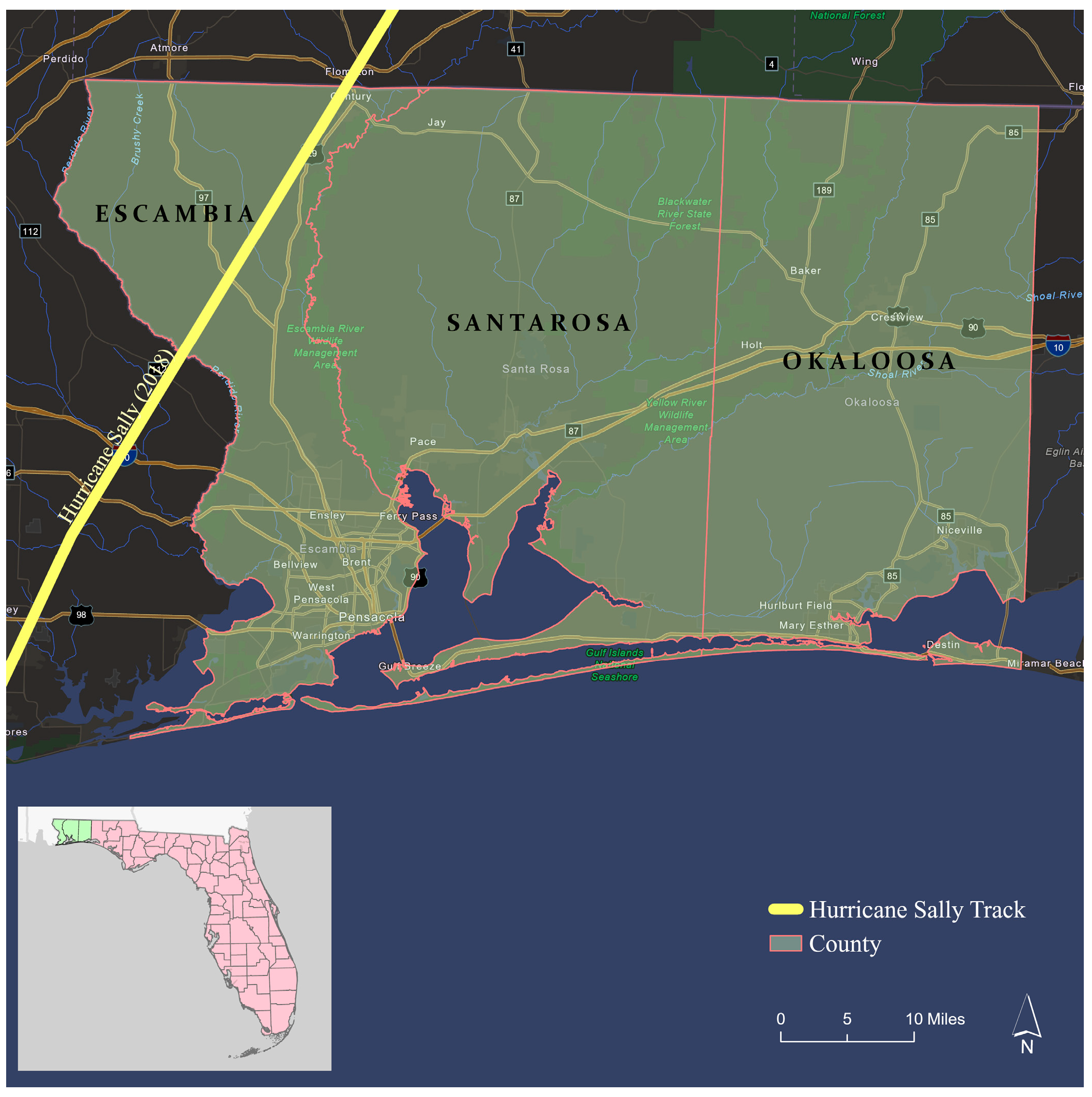
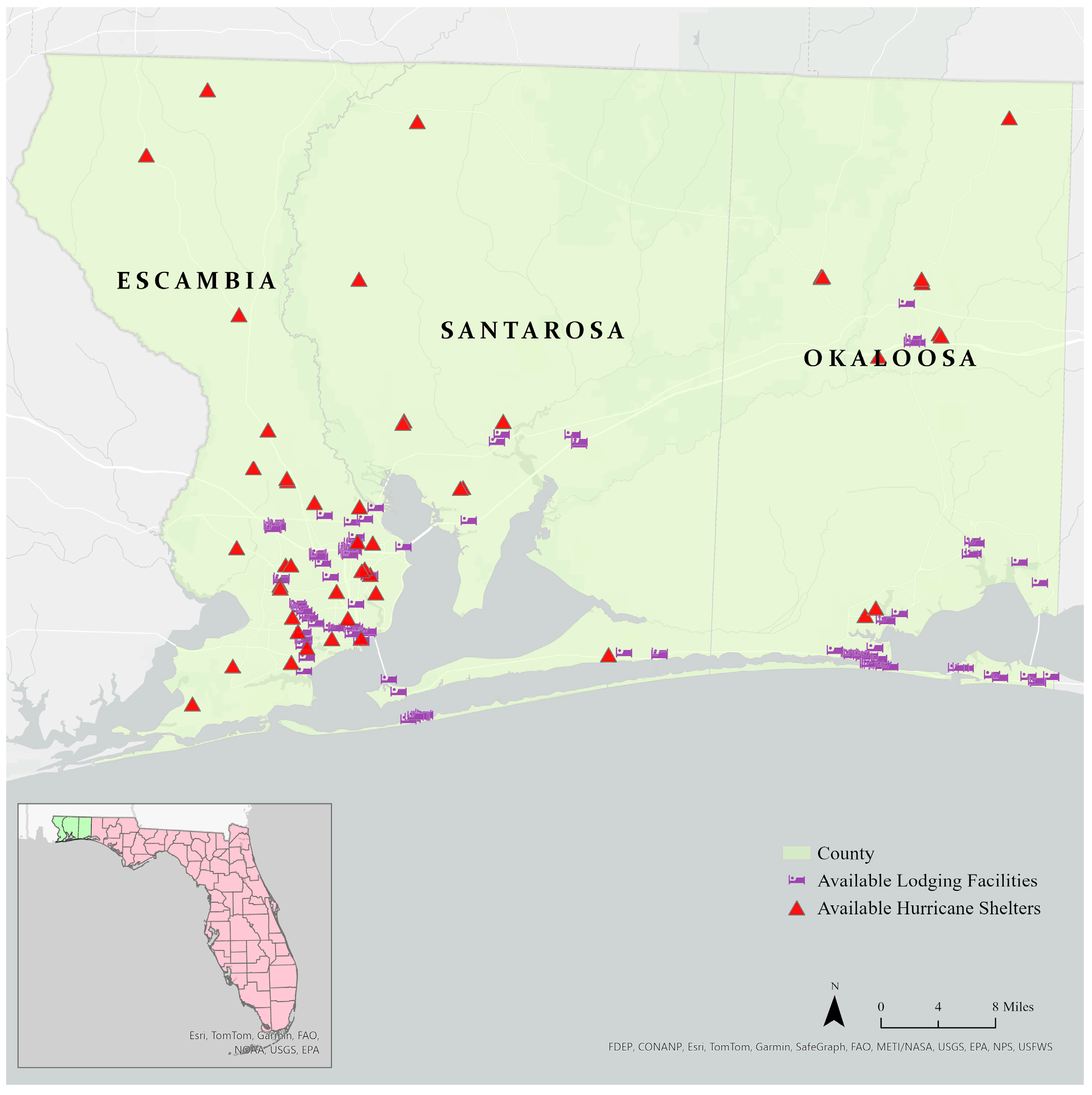
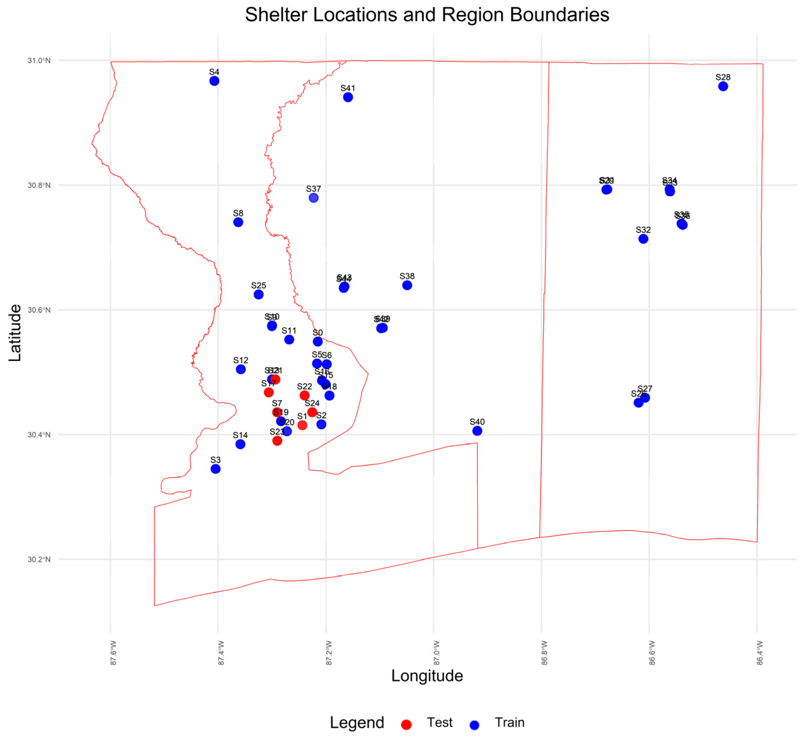
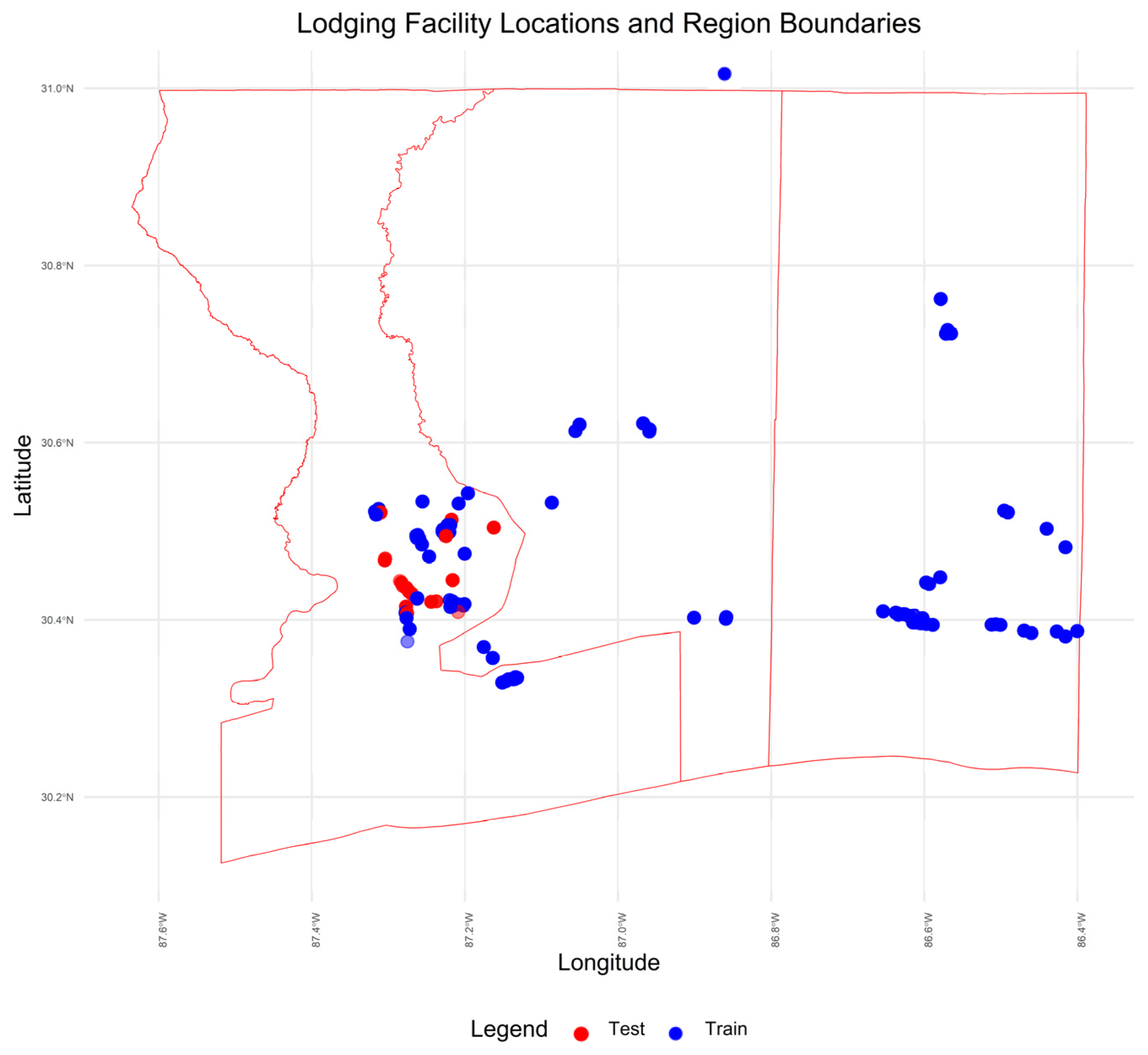
2.1. Study Region and Dataset

Hurricane Sally made landfall on 16 September 2020, with an incident period between 14 September and 28 September, causing severe damage across parts of the State of Florida, particularly in the Panhandle. Following the storm, the US president issued a major disaster declaration on 23 September 2020, enabling federal assistance to support recovery efforts in the affected areas [31]. Figure 1 shows this study’s region of interest with the intersected Hurricane Sally track. Sally’s track passed diagonally across Escambia County from the middle of the southwest. It brought widespread winds and heavy rainfall that seriously impacted the western Florida Panhandle. Schools in several Northwest Florida counties were closed as a precautionary measure. Santa Rosa and Okaloosa counties resumed classes on 21 September, while Escambia County schools reopened on 23 September. These closures began on September 15 and were implemented to ensure student safety amid the storm’s impact. Exceptions were made for certain schools based on specific circumstances within the districts [32,33].
Ahead of the Hurricane Sally landfall, the Florida Governor issued Executive Orders 20-224 and 20-225 order, which officially declared a state of emergency in Escambia, Santa Rosa, Bay, Calhoun, Franklin, Gadsden, Gulf, Holmes, Jackson, Liberty, Okaloosa, Walton, Washington counties [34]. The orders mandate that all public facilities, including elementary and secondary schools, community colleges, and state universities, must be available as (congregate) shelters upon request by local emergency management agencies. In addition, due to the concurrent public health emergency due to the ongoing COVID-19 pandemic, the executive order also included provisions for the state officials to activate agreements to use hotels as non-congregate shelters to protect evacuees from potential virus exposure and to maintain social distancing.
The datasets used for this study consist of GPS movement data, shelter and lodging facility wait time, and vehicle count data for 44 shelters and 123 lodging facilities in Florida’s Santa Rosa, Escambia, and Okaloosa counties from 01 to 30 September 2020. The geographical location and capacity information for each of these facilities were sourced from [35]. It is important to note that the dataset covers approximately 11% of Florida’s total registered vehicles, based on the data provider’s fleet coverage. While this represents a subset of the population, it captures a broad spatial distribution across the study region, ensuring key evacuation routes and urban-rural movements are reflected. The dataset includes personally owned vehicles, likely including those used for Uber and ride-sharing services. It includes various vehicle types, such as 11.8% sedans, 54.5% SUVs/MPVs, and 26.5% pickup trucks, though exact breakdowns remain anonymized. The dataset does not include government and emergency vehicles. Given this limitation, potential biases in vehicle representation are acknowledged. However, it is important to highlight that similar studies have effectively utilized datasets with significantly lower rates. For example, Dimitrijevic et al. [36] reported penetration rates between 2.31% and 4.39% in New Jersey and found them sufficient for robust traffic analytics. Hunter et al. [37] observed median penetration rates of approximately 4.5% across Indiana, Ohio, and Pennsylvania, confirming their adequacy for performance evaluations. Mathew et al. [38] used connected vehicle data with 3–5% penetration to analyze speed compliance in work zones. Given that our dataset’s 11% coverage exceeds these benchmarks, we believe it offers a robust and representative sample for modeling evacuation behaviors. Additionally, due to privacy concerns, no information can be extracted from the vehicle ID numbers provided. Figure 2 shows the lodging facility and shelter locations considered in this study.

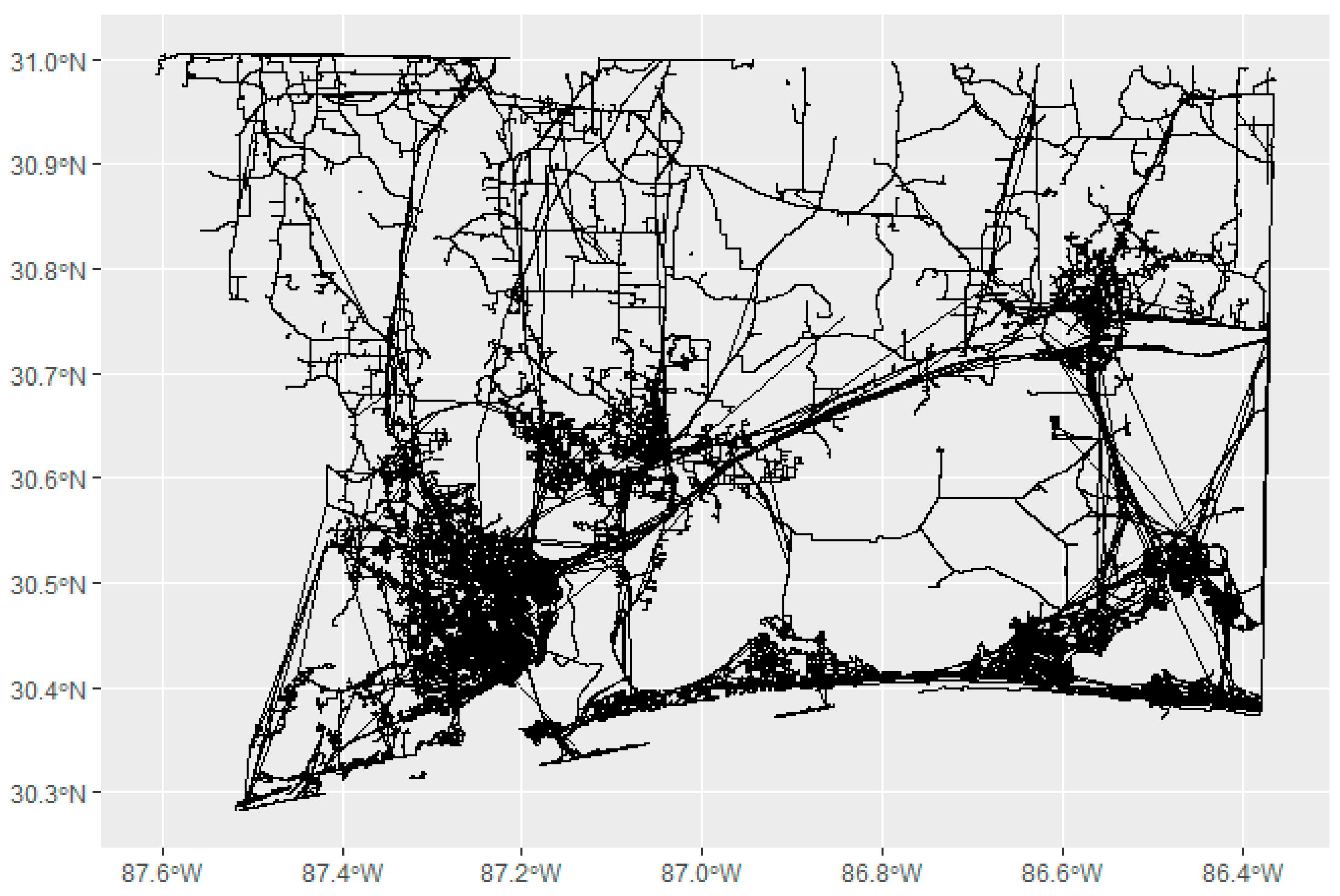
2.2. Data Processing

The vehicle trajectory data includes a series of waypoints with the details of vehicle paths within the geographic boundary of three counties: Escambia, Okaloosa, and Santa Rosa. Each waypoint contains detailed information, including geographic coordinates, timestamp, speed, ignition status, and a unique anonymous journey identifier. From 1 to 30 September 2020, there were 2,930,724 journeys with 1,078,927,715 waypoints. Figure 3 is a schematic representation of the journeys recorded during the period under review.
Since the data is anonymized, individual trip chains forming a journey are not explicitly declared, meaning that multi-stage evacuations and intermediate stops cannot be directly traced. To reconstruct probable trip sequences, a spatiotemporal grouping technique was proposed, allowing the identification of linked trips based on spatial and temporal proximity. We first define: (1) Start Location ( x s , y s ) and end location ( x e , y e ) of each trip, (2) Start time ( t s ) and end time ( t e ) of each trip and (3) Start ( I s ) and ending ( I e ) ignition status (i.e., whether the vehicle was turned on or off) for each trip. The trips that constitute a journey are matched and considered part of the same journey if it satisfies the following three conditions:
  • Spatial Matching Condition: The end location ( x e , y e ) of one trip must spatially match the start location ( x s , y s ) of the next trip.
  • Temporal Precedence Condition: The start time ( t s ) of the second trip must be chronologically after the end time ( t e ) of the first trip.
  • Ignition Status Verification: The first journey must end with I e = “key-off”, and the second trip must start with I s = “key-on”, ensuring a logical vehicle stop before the subsequent trip.
Table 1 summarizes the durations of the journeys obtained by the proposed trip chain forming method, summarized by destination county and whether they occurred during the school closure period. The total duration for the recorded journeys/trips is 946,291.2 h. About 6% of the recorded trips ended in counties outside the specified region of interest. The average trip duration within the region is about 0.3 h regardless of the county or the school closure status. However, during the school closure week, the total duration of trips shows a marked decrease (accompanied by a notable increase in the standard deviation) in all counties, as expected. The journeys that ended outside the region of interest have somewhat longer average duration of about 0.45 h. To analyze vehicle movement related to critical facilities (shelters and lodging locations), matched start and end points were intersected with facility ownership parcels. Parcel data was used to ensure accurate facility assignments, including parking lots and designated waiting areas, and reduce false matches that might occur if a vehicle stopped near but not inside a facility. Figure 4 illustrates the start and end points of two journeys mapped onto facility parcel boundaries.
To determine vehicle counts, only journeys that ended within facility parcel boundaries were considered, ensuring vehicles that arrived at shelters or lodging facilities were accurately counted. Each journey was treated as an independent event for vehicle count predictions, regardless of multi-stage evacuations, enabling precise aggregation for demand modeling and analysis. By leveraging spatiotemporal grouping, this study partially overcomes anonymization constraints and provides insights into evacuation movement patterns despite the lack of direct vehicle tracking.

2.3. Generalized Additive Model (GAM) Implementation

A GAM was fitted to model vehicle counts as a function of spatial coordinates (longitude and latitude), day of the month, day of the week, and the spatial basis functions. The choice of GAM allows for including non-linear relationships between the predictors and the response variable (vehicle counts). The GAM model utilized Gamma distribution with a log link function. The model can be expressed as in Equation (1):
log V ( x , y , t ) = β 0 + i = 1 7 β i z i + γ w + s x , y + s t  
where V ( x , y , t ) represents the vehicle count at the shelter/facility located at longitude, latitude pair ( x ,   y ) on day t ; β 0 is the intercept; z 1 ,   z 2 ,   z 3 , , z 7 are (0, 1) dummy variables indicating the day of the week; w is a (0, 1) dummy variable indicating whether the school closure is in effect on day t; β i z i represents the effect of each day of the week; γ w represents the school closure effect; s ( x ,   y ) and s ( t ) are smoothing spline functions for spatial coordinates and temporal dimension (days), respectively [39].
The GAM model (1) captures the evolving dynamics of evacuation-related shelter demand over space and time using spatial and temporal smoothing splines s ( x , y ) and s ( t ) , respectively. The spline functions further allow to interpolate or forecast non-linear trends over space and time [39]. The categorical variable β i z i accounts for day of the week cyclical effects (i.e., differences in mobility patterns between weekdays and weekends) and the categorical variable γ w accounts for the effect of school closure on shelter demand over time. By utilizing these components our model is able account for deterministic temporal dependencies. However, if stochastic temporal dependencies in the data are also deemed to be significant, they can be incorporated in the proposed GAM model by including autoregressive terms [39], in a relatively straightforward way.
The Generalized Additive Model (GAM) used in this study incorporates smoothing spline functions s ( x ,   y ) and s ( t ) to account for spatial and temporal variations in vehicle counts. These smoothing functions allow for the modeling of nonlinear relationships by balancing the trade-off between model flexibility and smoothness [40]. For the smoothing spline s ( x ,   y )   for the spatial coordinates, the following objective function is minimized:
min s i = 1 n y i s x i ,   y i 2 + λ s x ,   y 2 d x d y
where y i = log V ( x , y , t ) . The first term ensures a good fit to the observed data, and the second term imposes a penalty λ   to discourage roughness in the function s ( ) . The roughness penalty is quantified by the integral of the squared second derivative s ( x ,   y ) , which measures the curvature of the function. For the temporal smoother s ( t ) a similar minimization problem is solved. Therefore, the solution of the optimization problems yields the penalty terms λ = λ L a t L o n for the spatial smoother and λ = λ D a y for the temporal smoother. The parameter λ governs the trade-off between these two terms [40] as follows:
Low λ (High Flexibility): When λ is small, the penalty for roughness is minimal, allowing the function g to follow the data closely. In this case, the fit can become overly flexible, leading to potential overfitting. For example, the function might interpolate all data points, resulting in high variance but low bias [40].
Intermediate λ : By carefully tuning λ , a balance is achieved between fitting the data well and ensuring the function remains smooth enough to generalize to unseen data. This balance reflects the bias-variance trade-off inherent in statistical modeling [40].
High λ (High Smoothness): When λ is large, the penalty for roughness dominates, forcing g to become smoother. At the extreme, s ( . ) reduces to a simple linear function (or a straight line). This results in low variance but high bias [40].
In this study, the optimal values of λ for s(x, y) and s(t) were chosen through leave-one-out cross-validation (LOOCV). This approach evaluates the performance of the model by minimizing the cross-validated residual sum of squares (RSS):
RSS cv λ = i = 1 n y i g λ ^ x i 1 S λ , i i 2
where S λ is the smoothing matrix associated with the fit and S λ , i i represents its diagonal elements. LOOCV is computationally efficient for smoothing splines, as it avoids the need to refit the model repeatedly by leveraging the properties of S λ . A crucial byproduct of λ is its control over the effective degrees of freedom (EDF), which measure the complexity of the fitted function. For smoothing splines, the EDF is computed as:
E D F = i = 1 n S λ , i i
where a higher EDF indicates greater flexibility in the model. As λ increases, the EDF decreases, reducing the complexity of the fit. This study explicitly reports the EDF for each smoothing function to ensure interpretability and transparency in the modeling process [40].
For the spatial smoothing function s ( x ,   y ) , the penalty term λ L a t L o n controls smoothness along latitude and longitude values to ensure that the model captures key spatial patterns, such as high-demand regions for shelters, while avoiding overfitting to noise. A higher λ L a t L o n results in smoother spatial surfaces, reducing the risk of overfitting to local noise, while a lower value allows the model to capture finer spatial details, such as localized demand hotspots. Similarly, for the temporal smoothing function s ( t ) , the penalty term λ D a y controls the model’s sensitivity to daily trends in vehicle counts. This parameter ensures a balance between identifying meaningful temporal patterns (e.g., evacuation peaks) and avoiding overfitting to random daily fluctuations.
The smoothing parameters ( λ ) were optimized using Leave-One-Out Cross-Validation (LOOCV) approximated by the efficient Generalized Cross-Validation (GCV) criterion, as implemented in the mgcv package (version 1.9-1) in R [41]. The optimization focuses on minimizing the Penalized Residual Sum of Squares (PRSS) to balance model fit and smoothness. To ensure computational efficiency, the model uses Penalized Iteratively Reweighted Least Squares (P-IRLS) for convergence, which allows efficient optimization even with multiple smooth terms. Smoothing parameters for spatial ( λ l a t l o n ) and temporal ( λ d a y ) effects were tuned to prevent overfitting while capturing key spatial-temporal patterns in evacuation behavior.
Prediction of demand in unobserved facilities: Once Equation (1) is estimated from data using statistical methods, the estimated coefficients, β 0 , β 1 ,…, β 7 ,   γ , penalty terms λ L a t L o n , λ D a y and smooth functions s ( x ,   y ) and s ( t ) will be available. Using these estimated quantities, the vehicle counts for a given spatial coordinate ( x ,   y ) and day ( t ), and the basis functions will constitute our predictions.
Model Evaluation: The performance of the model was evaluated using summary statistics, namely the Pearson’s Correlation Coefficient (5), Root Mean Squared Error (6), Mean Absolute Error (7), and Mean Absolute Percentage Error (8), and visualizations, including actual vs. predicted train and test datasets plots.
CORR = X i X ¯ Y i Y ¯ X i X ¯ 2 · Y i Y ¯ 2
where C O R R is the Pearson’s Correlation Coefficient, X i are the actual data, X ¯ is the mean of the actual data, Y i is the predicted data, and Y ¯ is the mean of the predicted data.
R M S E = 1 n i = 1 n Y i Y ^ i 2
M A E = 1 n i = 1 n | y i ^ y i |
M A P E = 100 n i = 1 n y i y i ^ y i
where n is the number of observations, Y i are the actual values and Y ^ i are the predicted values.
Spatiotemporal Prediction: One of the major benefits of the proposed modeling approach is its ability to predict the number of vehicles at sites (shelters or lodging facilities) for which there are no historical data, and such predictions can be made into future time periods. To generate predictions, a spatiotemporal prediction grid was designed to cover the study area and time period. This grid allows vehicle counts at shelters and lodging facilities to be predicted across different spatial and temporal points. The predicted vehicle counts were then visualized using GIS tools, which helped identify hotspots of shelter demand. These visualizations are crucial for emergency management, enabling authorities to allocate resources more effectively and anticipate areas where shelter demand may exceed capacity.
By integrating these methodologies—spatiotemporal modeling, GAM, and detailed data processing—the study presents a robust framework for predicting and planning for non-congregate and congregate shelter demand. This approach can be adapted to other regions and disaster scenarios, providing a valuable tool for emergency management and resource allocation.

2.4. Justification of the Model Choice

Several advanced machine learning and simulation-based approaches exist for spatiotemporal disaster modeling, including convolutional neural networks (CNNs), recurrent neural networks (RNNs), and agent-based models (ABMs). While these methods have demonstrated effectiveness in prior disaster response studies [22]. Given the need for a transparent, interpretable model to inform real-time decision-making, we opted for Generalized Additive Models (GAMs). GAMs provide flexibility to modeling the complex spatial and temporal interactions in evacuation behaviors, while providing interpretability, making them suitable for impact analysis in policymaking applications. Table 2 summarizes a comparative evaluation of these modeling approaches.
GAMs provide an optimal balance between model complexity, interpretability, and computational efficiency, making them particularly suitable for policy-driven evacuation modeling where transparency is crucial. However, future research could explore hybrid models that combine GAMs with deep learning approaches.

2.5. Benchmark GLM for Comparative Study

As a benchmark approach to compare efficacy of the proposed GAM based demand prediction, we also implemented a Generalized Linear Model (GLM). Consistent to approach, GLM model predicts the vehicle counts as a function of spatial coordinates (longitude and latitude), day of the month, and the day of the week:
log V ( x , y , t ) = β 0 + β 1 x i + β 2 y i + i = 1 7 β i z i + β 3 γ w + β 4 t
GLM model also utilizes a Gamma distribution with a log link function, which is suitable given the positively skewed nature of the vehicle count data. However, in contrast to our GAM approach, GLM is not able to interpolate complex spatial-temporal patterns. Nevertheless, the GLM model served as a foundational comparison point to evaluate the efficacy of more flexible modeling approaches.

3. Results

The testing set was randomly selected from areas on the map with a high concentration of shelters and lodging facilities. Specifically, it included the following shelters: S1, S7, S17, S21, S22, S23, and S24, and the following lodging facilities: L1, L2, L3, L4, L12, L22, L23, L28, L29, L30, L53, L56, L57, L58, L60, L63, L71, and L73. The remaining data, consisting of 37 out of the 44 shelters and 105 of the 123 lodging facilities, was used for training. The data was analyzed using the method described in Section 2, and predictions were made using the model defined in Equation (1) for the GAM model and Equation (9) for the benchmark GLM. Table 3 presents the features used in the dataset along with their respective units of measurement. Note that the proposed GAM models evacuation and sheltering dynamics on a daily basis; therefore, vehicle counts at the facilities are aggregated daily. This daily sampling provides sufficient temporal resolution for emergency management decision-making. Table 4, Table 5, Table 6 and Table 7 summarize the results of the GAM and GLM models using the training and testing datasets for lodging facilities and shelters. Numbers in brackets indicate the p-value of the correlation estimates. A p-value higher than 0.05 mean correlation is not significantly different from 0 at the 0.05 level of significance. It can be seen that the negative correlation estimates have large p-values and are not different from 0.
The results of the GAM model indicate that the model performs better for lodging facilities compared to shelters, as evident from the metrics in both tables. For lodging facilities, the training and testing RMSE values are 4.034 and 3.421, respectively, showing reasonable prediction errors, with the test dataset having slightly lower errors. The correlations (0.5485 for training and 0.2096 for testing) show a moderate predictive performance for the training set and a weaker performance for the test set. However, the MAPE values (108.76% for training and 113.80% for testing) highlight room for improvement in predicting relative errors.
For shelters, the training and testing RMSE values are 6.7791 and 7.7213, respectively, suggesting higher prediction errors compared to lodging facilities. The correlation for training data is strong (0.8593), indicating a positive relationship between predicted and actual values, but the test set shows zero correlation (-0.0835 but insignificant), suggesting low generalizability of the model for shelter predictions. Additionally, the MAPE values (79.41% for training and 107.01% for testing) further emphasize the challenges in achieving accurate relative predictions for shelters.
Compared to the benchmark GLM method (Table 4 and Table 5), the proposed GAM approach (Table 6 and Table 7) has significantly improved predictive accuracy for both shelters and lodging facilities with respect to all performance measures. The GAM model showed superior performance in comparison with the benchmark GLM. Notably, the GAM significantly reduced RMSE and MAE across both shelters and lodging facilities. For shelters, the GAM achieved a training correlation coefficient of 0.8593, a substantial improvement over the GLM’s 0.1760. Similarly, for lodging facilities, the GAM outperformed the GLM with better RMSE, MAE, and correlation metrics. The GAM’s flexibility in modeling nonlinear patterns and its capacity to incorporate spatial and temporal smoothing functions resulted in more accurate and generalizable predictions.

3.1. Effects of Data Normalization on Model Performance

To account for differences in facility size and population across counties, we further studied the effectiveness of normalized performance metrics of demand predictions at shelters and lodging facilities. Specifically, actual and predicted vehicle counts were normalized by facility capacity (total spaces available at each facility). To compare results from different counties we computed scaled root mean square errors (SRMSE), which is defined as RMSE divided by the standard deviation. This enables us to compare the prediction accuracies in counties with varying shelter or lodging capacities on an equal basis. Equations (10) and (11) show SRMSE with actual data and normalized data based on facility capacity, respectively.
S R M S E = 1 n i = 1 n y i ^ y i 2 Var y
S R M S E N o r m = 1 n i = 1 n y i ^ / C i y i / C i 2 Var y / C
where y i and y i ^ represent the actual and predicted vehicle counts at the observation i , respectively. C i denotes the facility capacity (total spaces available at the shelter or lodging facility) corresponding to the observation i .
Table 8 and Table 9 show the prediction SRMSE and S R M S E N o r m results for shelters and lodging facilities, respectively, within the three counties, as well as the populations, available spaces in the facilities, the total counts of vehicles that visited the facilities during the study period in each county and the vehicle count per available space (Veh Ct/Av Sp). In contrast to RMSE (see Table 6 and Table 7) which is higher for shelters, the SRMSE values overall are smaller for shelters than lodging facilities. This is because SRMSE measures prediction errors as a multiple of standard deviation and the shelter data has higher variability. S R M S E N o r m which uses predictions normalized by facility size provides further ability to compare counties with varying available spaces.
SRMSE results indicate higher prediction uncertainty for shelters in counties with fewer spaces, as expected. However, for lodging facilities SRMSE is not necessarily inversely proportional to available spaces. This is probably because shelters are better spread out geographically (see Figure 5) and smaller counties (by population) receive fewer vehicle counts per available spaces, as expected. By contrast, lodging facilities are highly clustered in the coastal areas, resulting in the unexpected behavior that smaller counties receiving larger vehicle counts per available space than larger counties (Santa Rosa receives larger traffic per available space then Okaloosa). The proposed S R M S E N o r m by contrast is better able to quantify prediction uncertainty for lodging facilities; for example, counties with larger more available spaces, such as Escambia has smaller S R M S E N o r m than those with fewer available spaces, such as Okaloosa. This further highlights the increased complexity of predicting lodging demand.
The high MAPE values (>100%) can be attributed in part to the unique circumstances during the COVID-19 pandemic, where lockdown restrictions, social distancing mandates, and heightened health concerns significantly influenced evacuation behaviors. These factors likely led to atypical and inconsistent evacuation patterns, with some facilities underutilized and others unexpectedly crowded, contributing to higher relative errors. In this analysis, we demonstrated that using prediction error measures based on normalized data can help mitigate, to some extent, the effects of varying sample sizes. However, as possible future research, more systematic strategies within the modeling framework, such as outlier mitigation, data normalization, and robust loss functions can be undertaken to reduce the impact of extreme variations and improve model resilience.
Overall, the model demonstrates better predictive accuracy for lodging facilities, while the performance for shelters requires significant refinement to improve robustness and reliability. The discrepancies in testing performance, particularly for shelters, suggest the need for further model calibration or additional data to enhance predictive accuracy. Figure 5 and Figure 6 depict the spatial distribution of the selected shelters and lodging facilities for the test and train datasets, with locations color-coded in red (test) and blue (train).
Figure 7a,b show actual vs. predicted vehicles for shelters and lodging facilities, respectively. The plots indicate that the model performs reasonably well for shelters and decently for lodging facilities throughout the study period, with many points lying close to the line of perfect prediction. There are instances where predictions deviate, indicating room for improvement. There seems to be a good match between actual and predicted values, especially for lower vehicle counts. However, for higher counts, the model occasionally underpredicts or overpredicts. However, the model struggles with the test data, as evidenced by a wider spread of residuals.

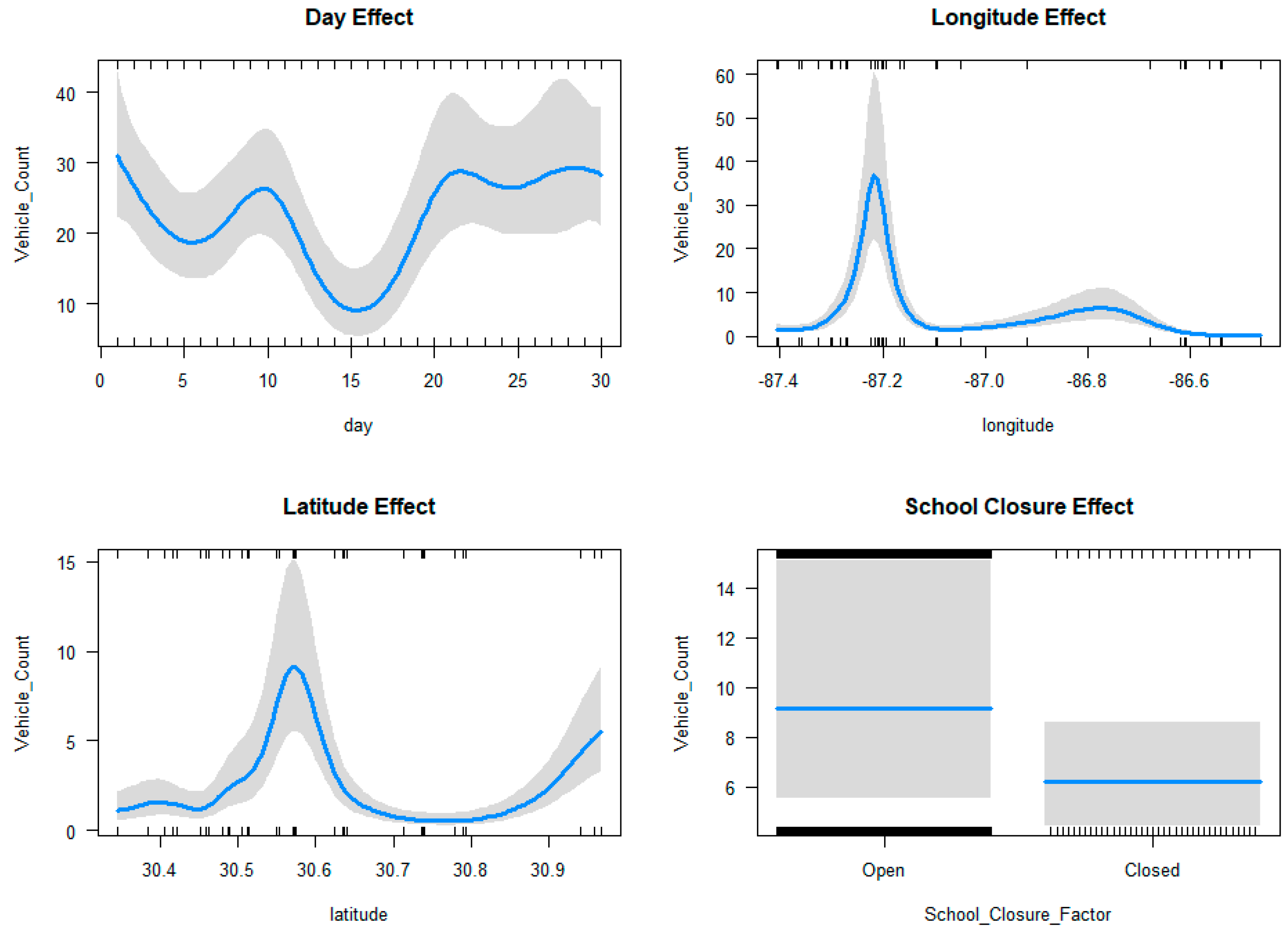
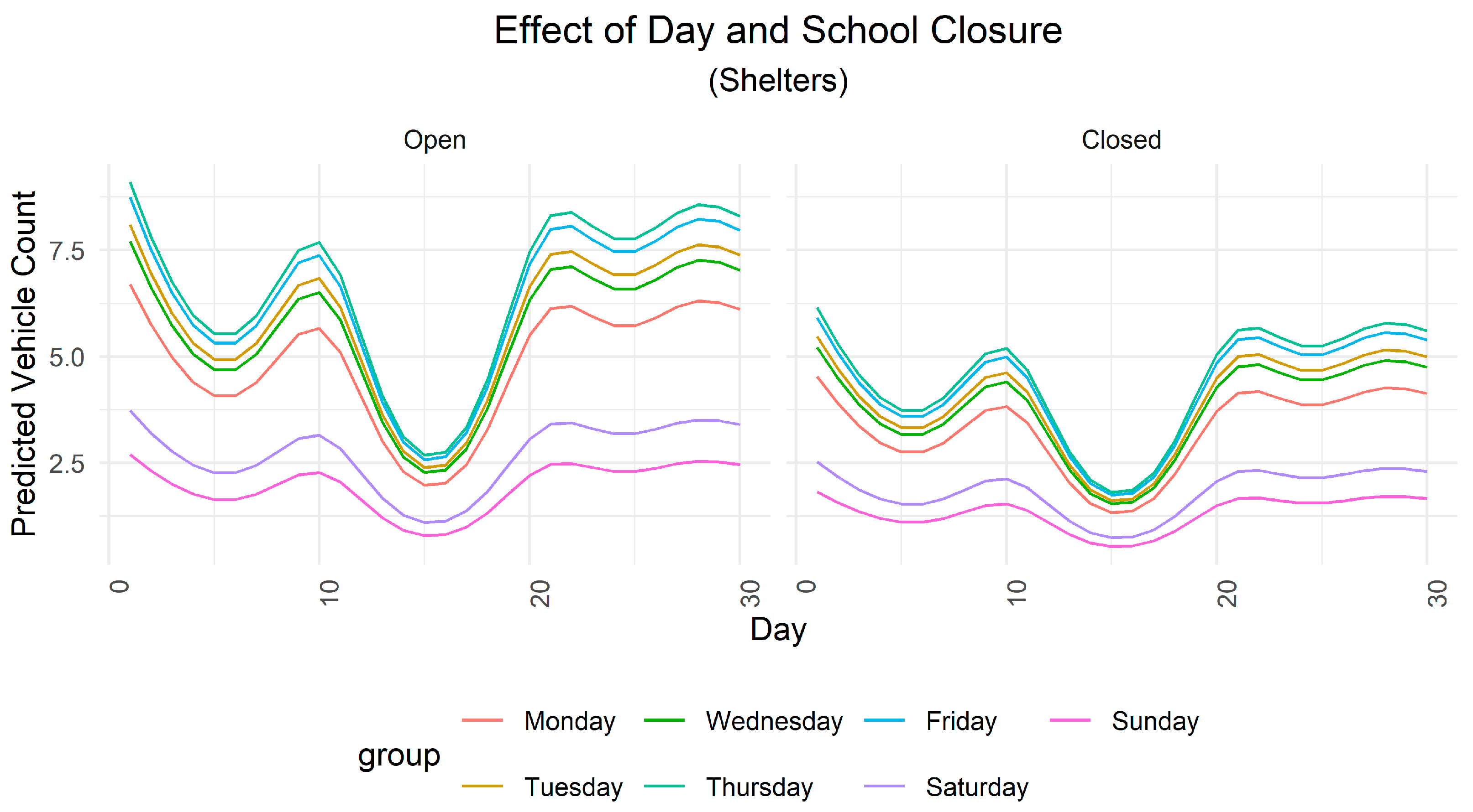
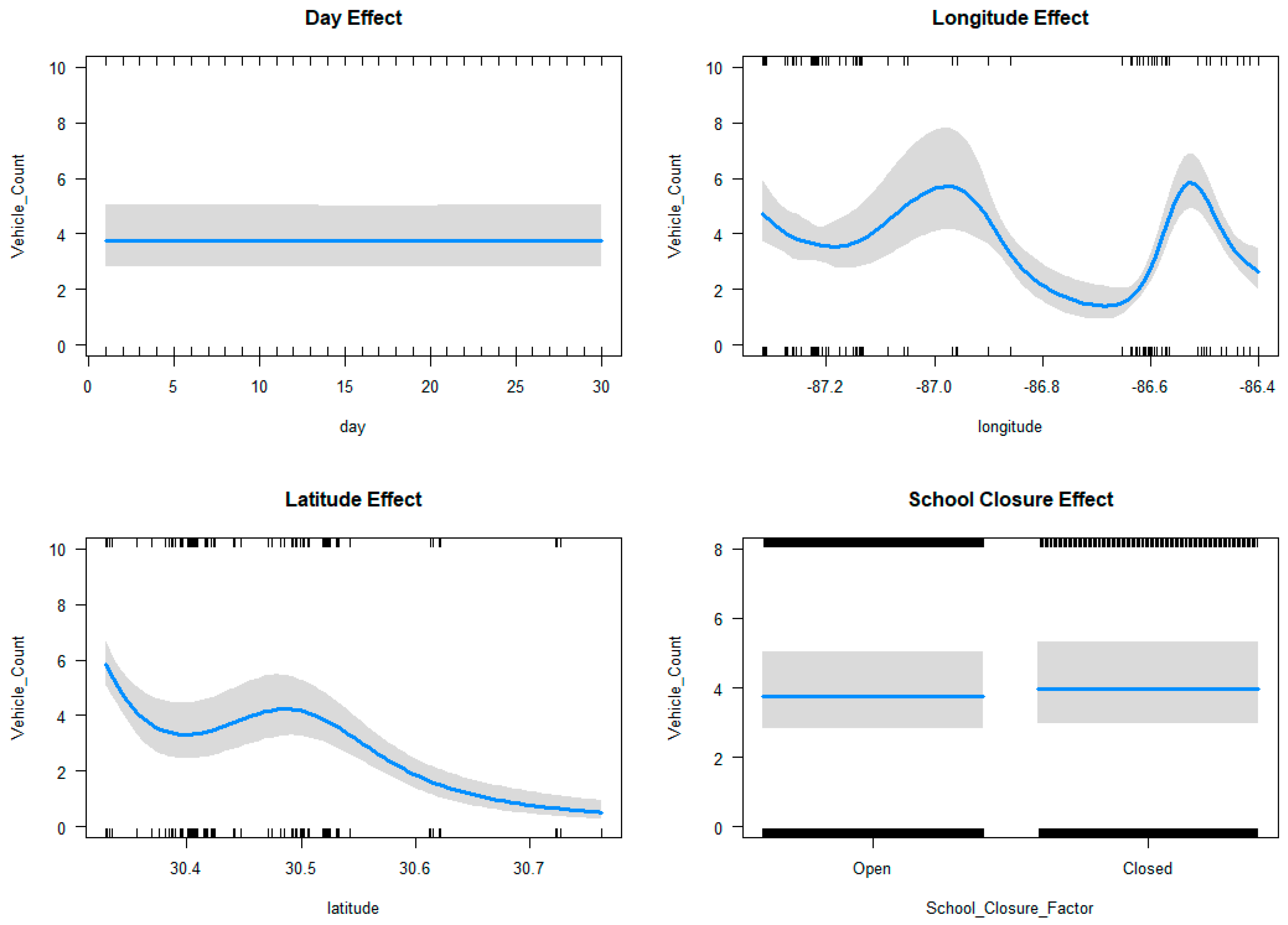
3.2. Effects of School Closure and Geographic Location on Shelter Demand

Figure 8 illustrates the effects of various factors on vehicle counts, as modeled by the Generalized Additive Model (GAM) for shelter data. The Day Effect shows a cyclical trend throughout the month, with a significant dip occurring around the middle of the month, which coincides with Hurricane Sally’s landfall period. Higher vehicle counts are observed at the start and end of the month. The relationship with longitude reveals a pronounced peak around -87.2, indicating a region with significantly higher vehicle counts. Beyond this peak, vehicle counts decrease sharply as longitude increases, suggesting spatial clustering or hotspot activity in specific areas. The latitude effect shows a nonlinear pattern with a prominent peak around 30.6, with additional increases at higher latitudes. The School Closure Effect indicates a significant reduction in vehicle counts when schools are closed, reflecting the impact of school operations on mobility. Figure 9 shows the interaction effect between the day of the week and school closure status. When schools are open, vehicle counts are higher on weekdays (Monday-Friday) and lower on weekends (Saturday and Sunday). This pattern indicates increased mobility during school days. When schools are closed, vehicle counts drop uniformly across all days, with a less pronounced difference between weekdays and weekends.
Figure 10 highlights the effects of various factors of the GAM model on lodging facilities. The Day Effect shows minimal variation in vehicle counts across the month, indicating a lack of temporal variability. The Longitude Effect shows a non-linear pattern with multiple peaks and troughs, indicating spatial variability in vehicle counts along the east-west axis. Peaks suggest hotspots with higher lodging demand, likely due to clusters of facilities or key evacuation routes, while troughs represent areas with lower activity. The Latitude Effect reveals an initial decline in vehicle counts as latitude increases, a slight rise around 30.5 (indicating a localized hotspot), followed by a steady decline northward. This suggests higher lodging demand in southern areas, with reduced activity further north, possibly due to fewer facilities or less evacuee movement. These patterns highlight key areas of lodging demand, helping emergency planners optimize resource allocation and evacuation strategies. The School Closure Effect shows stable vehicle counts regardless of school status, suggesting that school operations have limited influence on lodging-related mobility.
Figure 11 shows the effect of day and school closure status on lodging facilities. When schools are open, predicted vehicle counts remain stable across all days of the week, with Sunday showing a slightly higher count compared to other days. When schools are closed, the stability persists, with only minor differences in vehicle counts between weekdays and weekends. Figure 12b shows a nonlinear relationship between longitude and school closure status on vehicle counts for lodging facilities, with distinct peaks and troughs. Vehicle counts increase near longitude −87.0, peak just beyond this longitude, and decline sharply near −86.8, followed by another rise around −86.6. When schools are closed, vehicle counts are generally higher near −87.0 but slightly lower near −86.6 compared to when schools are open. This indicates that geographic factors are more critical in lodging-related mobility, while school closure status has a smaller, location-dependent effect.
The optimal penalty term λ for shelters and lodging facilities in Table 3 below, as discussed in Section 2.3, reveal key insights into the complexity and smoothness of the smoothing functions used in the Generalized Additive Model (GAM). These values indicate the trade-off between flexibility and smoothness in modeling various components of the data. The results highlight notable differences between shelters and lodging facilities in terms of spatial and temporal variability: Shelters have lower λ values to capture localized and dynamic patterns effectively. Lodging facilities show smoother, more uniform trends with higher λ values, reflecting less pronounced variability in space and time. The impact of school closures is more influential for shelters than for lodging facilities, where it has a negligible effect.
These findings emphasize the need to tailor smoothing parameters to the unique characteristics of each dataset to achieve an appropriate balance between flexibility and smoothness.
One of the unique insights derived from the proposed GAM approach is quantifying the effect of school closure on vehicle traffic in shelters and lodging facilities during this co-occurring hurricane pandemic emergency. The impact of school closure has varying effects on shelters and lodging facilities, as well as the spatial location. From Figure 12 and Table 10, the school closures had decreased the use of schools while it significantly increased the use of lodging facilities. These effects are significant at a 95% confidence level and can be attributed to the state of emergency declaration and the use of these facilities as shelters during the emergency. Figure 12a investigates the effect of longitude and school closure status on predicted vehicle counts. A sharp peak in vehicle counts is observed around longitude −87.25 when schools are open, indicating a concentrated hotspot of activity. When schools are closed, the peak is significantly reduced, but the general spatial pattern remains consistent. Beyond the hotspot, vehicle counts decrease consistently as longitude increases for both open and closed schools. These figures highlight the function of temporal, spatial, and school operations in shaping vehicle mobility patterns. We note that the effects plots display the marginal effects of each variable (or a combination of two variables, in the case of an interaction). The effect of a variable is obtained by averaging the predictions of the model for all the values of the remaining variables and therefore the predictions in these plots are non-integer values, even though they refer to number of vehicles. As shown in Figure 12b, the effect of school closures is more pronounced (greater distance between the two curves) in the western parts of the study region (west of −87.00 longitude), closer to the landfall area. This suggests that lodging facilities were used more frequently for sheltering in these areas.

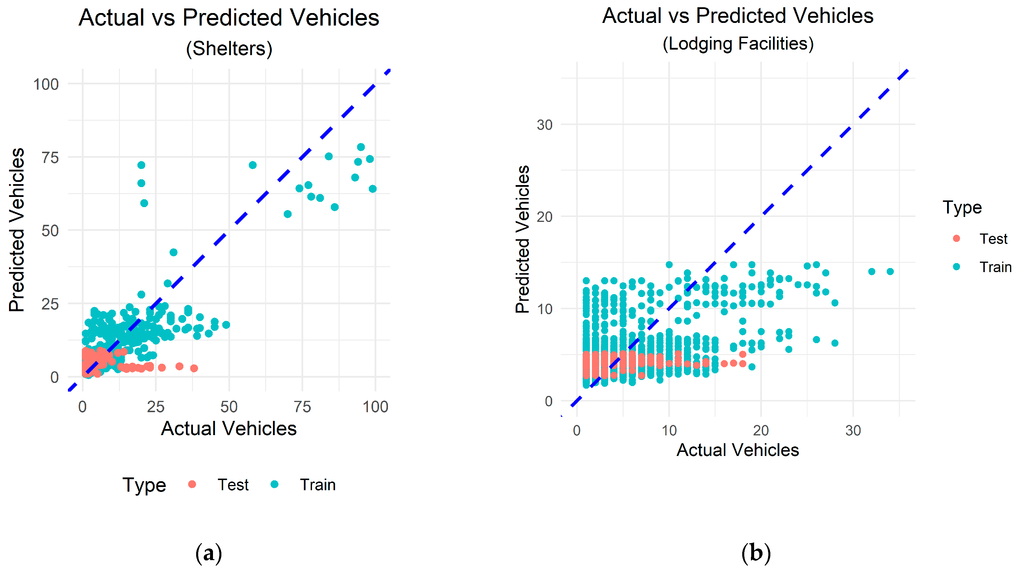
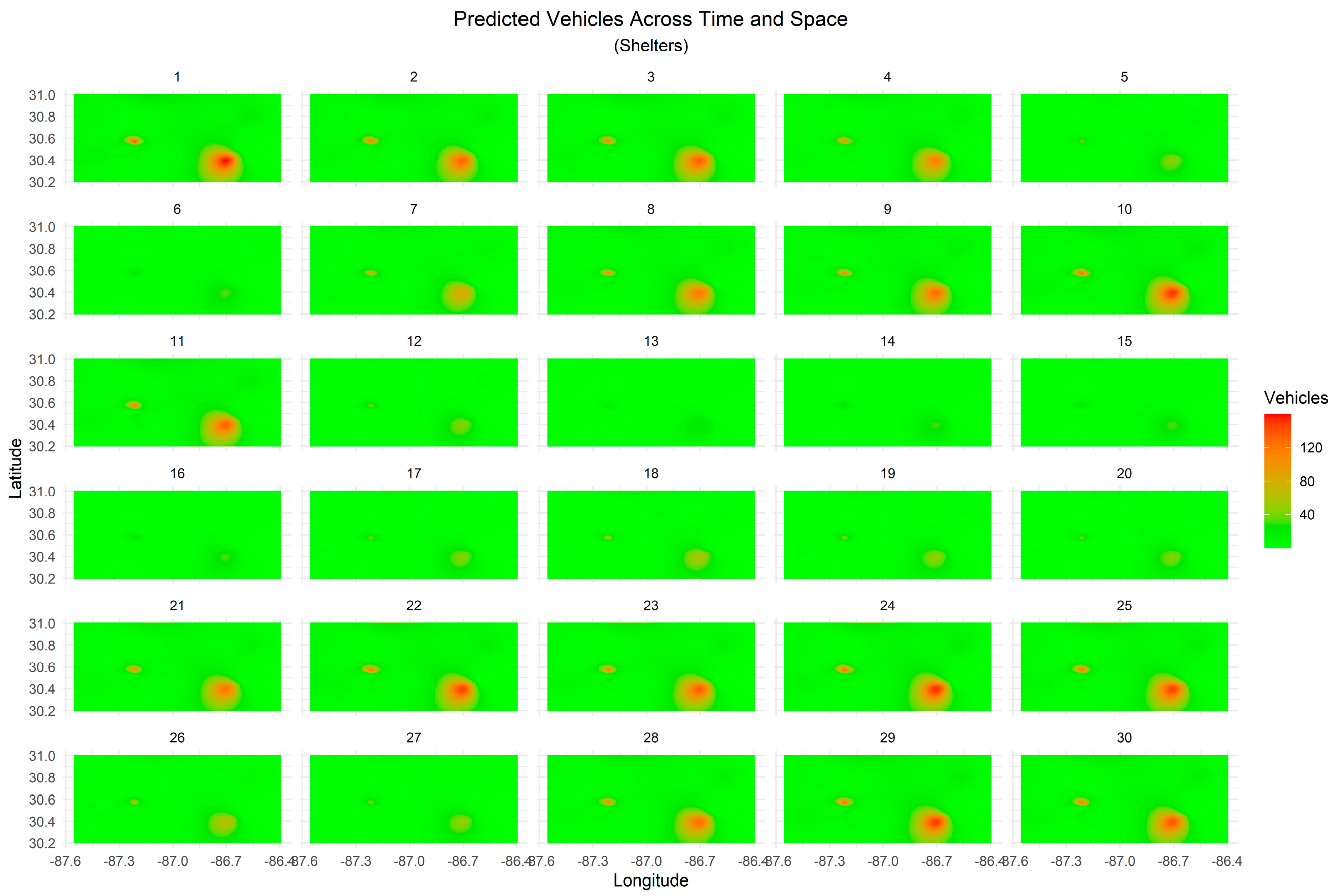
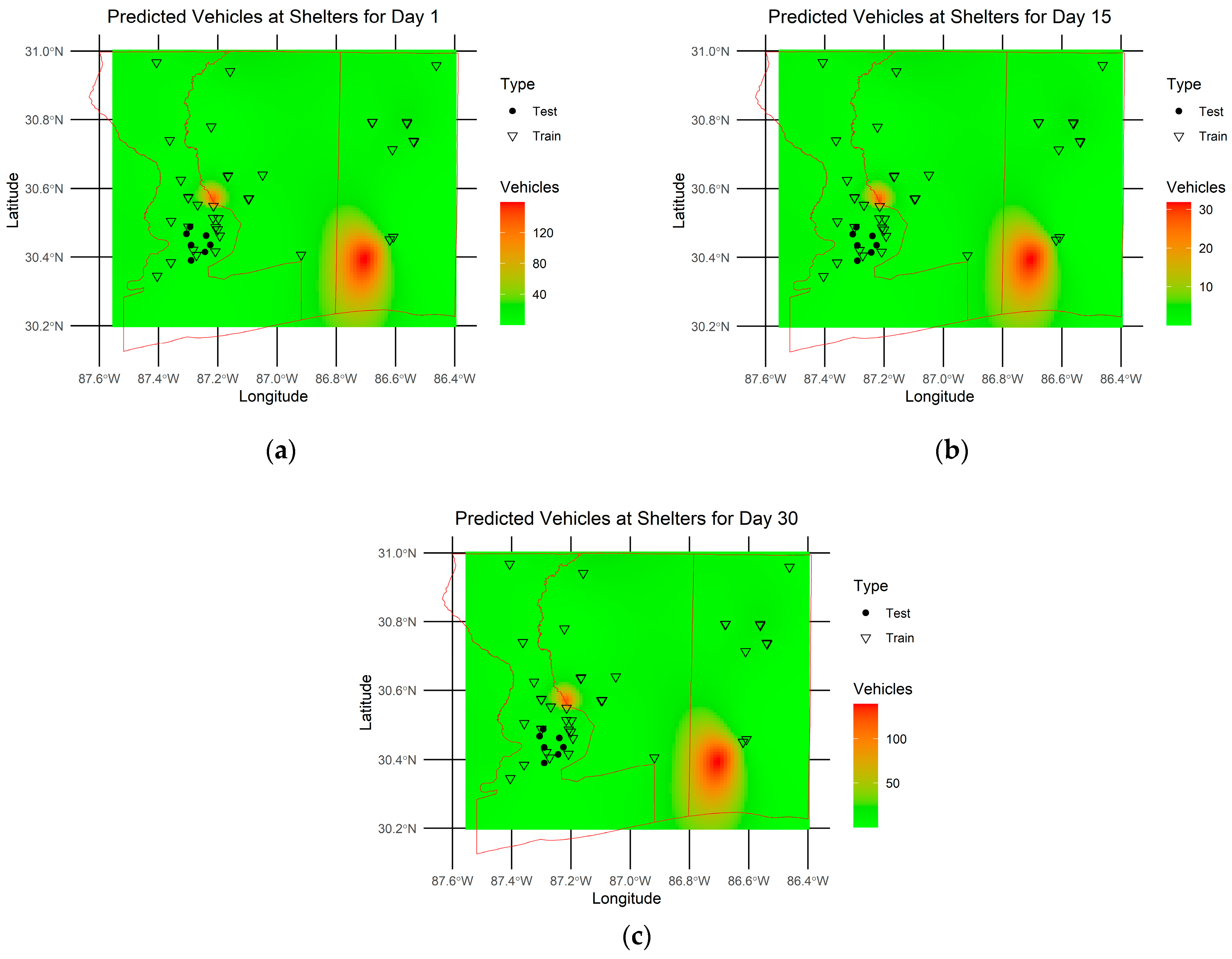
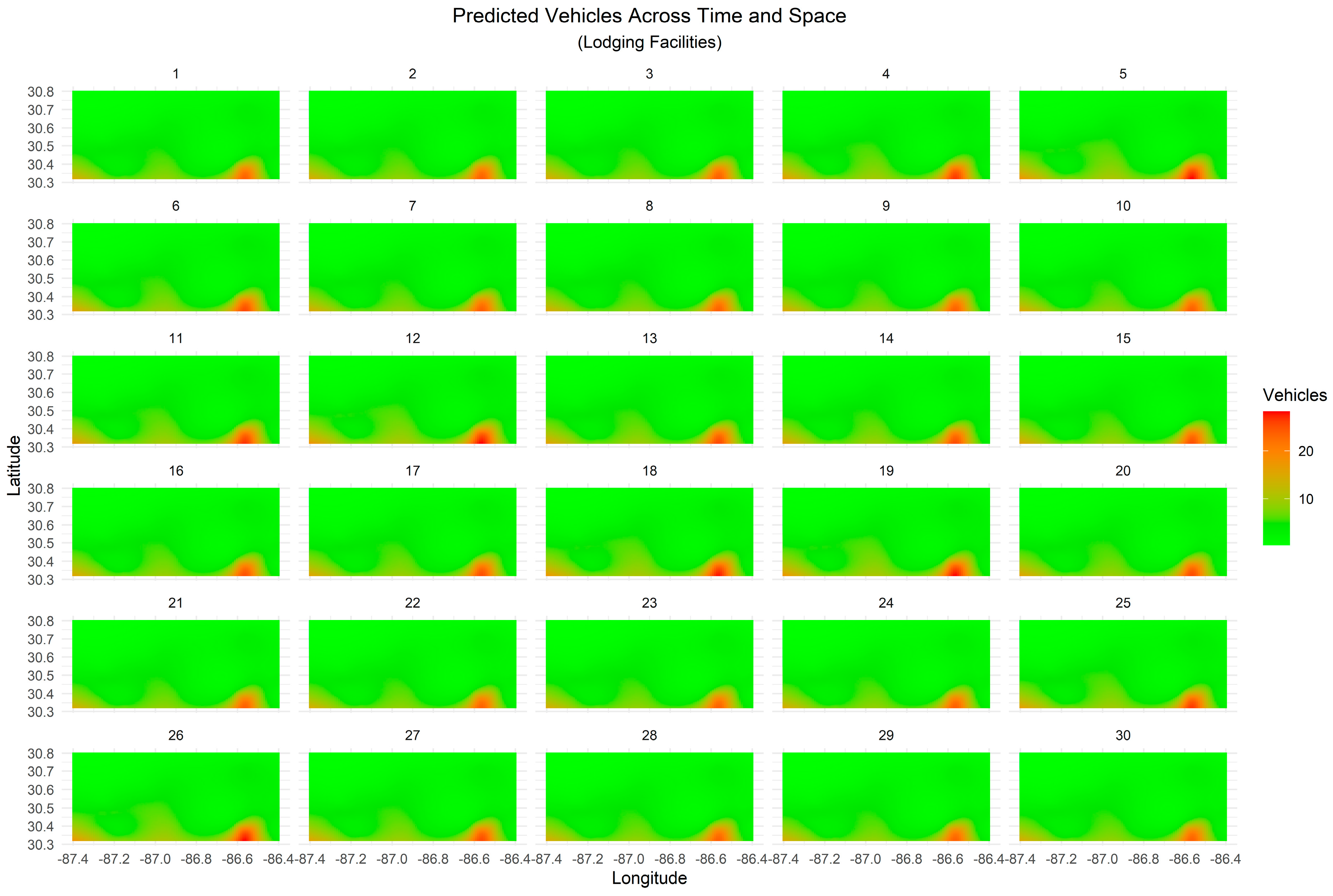
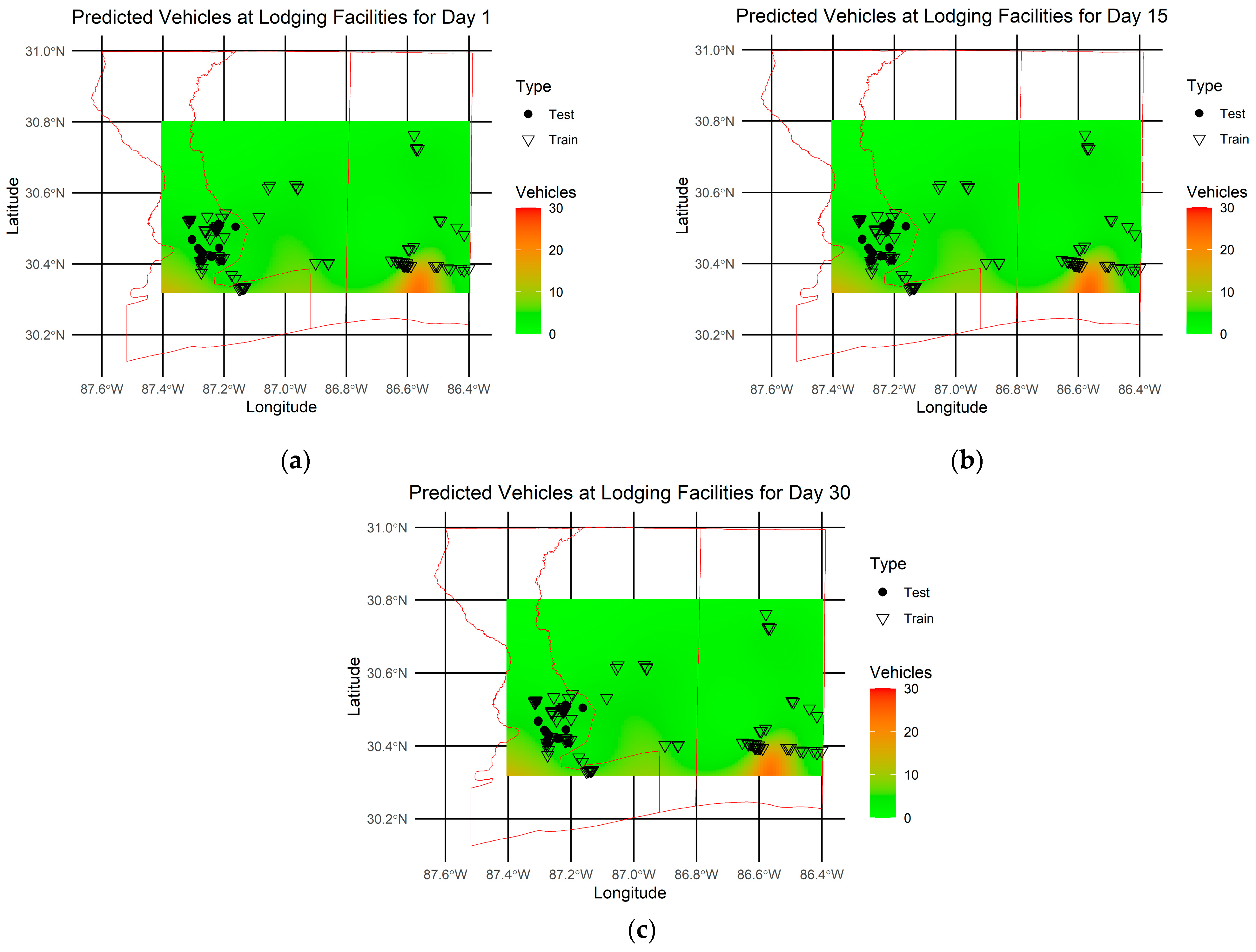
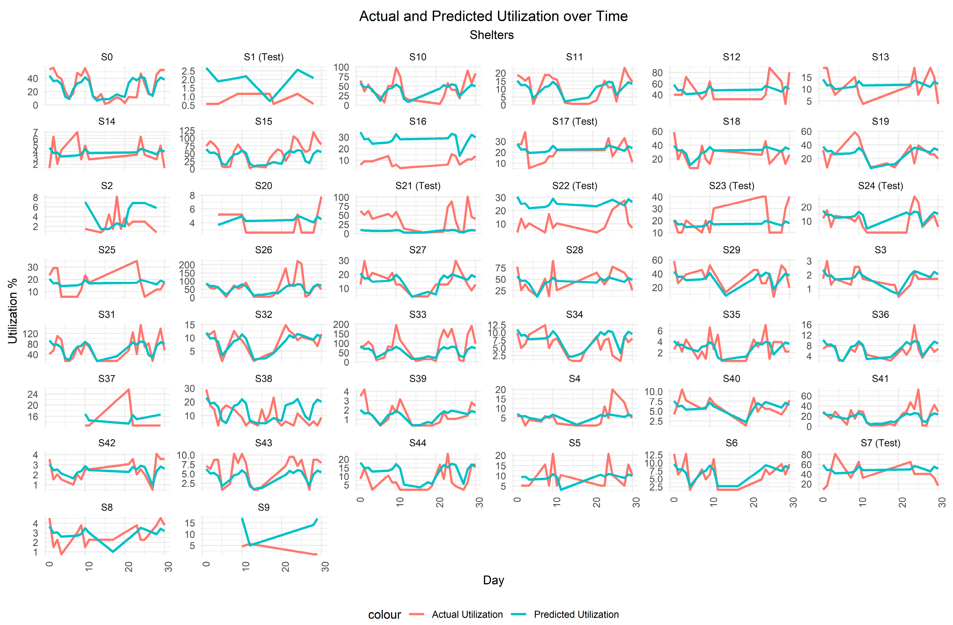
3.3. Spatiotemporal Demand Prediction

The spatiotemporal grid prediction approach (Section 2.3) is implemented to predict vehicle counts at shelters and lodging facilities across the study area. Using a spatial prediction grid and the GAM model, vehicle counts were visualized using GIS tools, identifying hotspots of facility demand. Figure 13 and Figure 14. Show heat maps for vehicle distribution patterns across the month. Day 1 saw peak vehicle counts, reflecting high initial demand. Day 15 showed reduced counts, coinciding with Hurricane Sally’s landfall, while Day 30 revealed partial recovery. Higher vehicle intensity near training zones indicates potential model biases or regional dynamics affecting predictions.
Figure 15 and Figure 16 are spatial heat maps showing the vehicle counts at the lodging facilities. The predicted vehicle distribution shows stable patterns over time, with most regions having low to moderate vehicle counts. Higher activity was concentrated around training facilities, with lower intensities at test areas, indicating model bias influenced by training data. This highlights the need for improved generalization to better predict vehicle dynamics in test regions.
These spatial heatmaps show the predicted demand across the entire study area, extending beyond the known facility locations. The model was trained on data from existing shelters and lodging facilities, and the heatmaps aim to highlight potential demand hotspots at both known and unknown locations. The concentration of demand near training zones partly reflects true evacuation patterns, as lodging facilities are typically located along primary evacuation routes. Because the GAM model interpolates over spatial coordinates, the predicted hotspots may not exactly coincide with existing facilities (in our case the hotspots correctly capture demand in larger facilities). Areas of high predicted demand without existing facilities highlight potential service gaps and can inform emergency planners about areas where additional resources may be needed, for example, for deciding on locations of new facilities.

3.4. Comparison of Predicted Demand and Available Capacity

Geyer and Ragland [45], showed that more than half of all trips in personal vehicles in the United States are taken in vehicles with multiple occupants and the mean vehicle occupancy rate is 1.63 persons. Based on this assumption and the fact that the dataset used in this study covers approximately 11% of the total vehicles in Florida, we can compare the actual and predicted utilization of each individual shelter for each day. The utilization rate was calculated as:
U t i l i z a t i o n   % = D e m a n d A v a i l a b l e   S p a c e s × 100
Figure 17 shows the actual and predicted utilizations of the shelters, obtained by using Equation (10). Note that for each facility Available Spaces is obtained from [35] and the predicted utilization is computed using the demand prediction from the proposed GAM approach (actual utilization is computed using the observed demand). In addition, the figure shows predicted utilization for both training data (used to build the GAM model) and test data (hold-out samples not used in model building). The predictions for test data (while they are inevitably poorer than those for the training data) agree reasonably well with the observed data (as evidenced with the good Test Data performance in Table 5 and Table 6) and are very useful in demonstrating the generalizability of the model in new or unseen conditions.
The predicted utilization closely follows the actual utilization across most shelters, indicating a generally good model performance. However, in shelters like S1, S21, and S22, the predictions show noticeable deviations, suggesting potential underfitting or overfitting or the need for additional features to capture these fluctuations better. While the model performs well in stable demand scenarios, further refinement is needed for shelters with more volatile utilization patterns.
As for the shelter analysis, the vehicle occupancy rate of 1.63 was adopted to estimate the demand at the lodging facilities. However, an additional assumption was made that each room at the lodging facilities could accommodate four people, which was used to adjust for the available capacity at the lodging facilities. While our vehicle occupancy assumption is empirically supported by literature, (see e.g., [45]), our room occupancy assumption could be refined with future research by surveying hotel/lodging data for average room occupancy during evacuations. Figure 18 compares actual and predicted utilization across multiple test lodging facilities over the period under review. These plots show that the prediction model, tested on a dataset not used during training, performs inconsistently, accurately predicting trends in some facilities but missing significantly in others.
The summary statistics in Table 2 further highlight the performance of the model. For the training dataset, the RMSE (4.0368) and MAE (2.7591) indicate moderate error levels, with a MAPE of 108.76% and a correlation of 0.5485, suggesting a fair alignment between actual and predicted demand. However, for the test dataset, the RMSE (3.4211) and MAE (2.57656) are slightly lower, but the correlation drops significantly to 0.2096, reflecting weak predictive performance on unseen data. Additionally, the MAPE for the test data rises to 113.80%, indicating the model struggles to generalize well beyond the training dataset.
Additionally, some days are missing from the plots for certain facilities due to the absence of available data for those periods. Facilities like L29 and L60 show relatively good model performance, while others like L4 and L3 exhibit discrepancies between actual and predicted utilization. Some facilities are underutilized, with capacity far exceeding demand, while others occasionally face demand that approaches or exceeds capacity, highlighting potential inefficiencies in resource allocation and the need for model refinement.

3.5. Model Performance on 15-Day Subset of the Training Data

To assess how the trained model performs when applied to a shorter observation window, we compared the GAM trained on the full 30-day period to a GAM trained using only the 15-day period from 08 September 2020 to 22 September 2020. The window included the 1-week school closure period plus another 8 days baseline period to estimate the school closure effects with a shortened data window. Table 11 and Table 12 summarize the performance metrics of the model from the smaller dataset. The model largely retained comparable predictive accuracy with the 15-day training period, closely matching the performance observed over the full 30-day period both for shelters (Table 6; training MAPE = 79.41%, test MAPE = 107.01%) and for lodging facilities (Table 7; training MAPE = 108.76%, test MAPE = 113.8%). This suggests at least 15 days of data is sufficient (as long as it includes the 1-week disruption period under study) to train the proposed GAM model to achieve an acceptable prediction accuracy for a study region covering 3 counties.

4. Discussion

The spatiotemporal modeling approach adopted in this study has shown significant effectiveness in predicting shelter demand during natural disasters. By integrating vehicle trajectory data with modeling techniques such as GAMs and Gaussian radial basis functions, the study was able to capture spatial and temporal dynamics that traditional models often overlook. The high correlation between predicted and actual vehicle counts, particularly for shelters, highlights the accuracy and reliability of this approach. However, the slightly lower performance of the model in predicting demand at lodging facilities suggests that additional factors may need to be considered in future iterations of the model.
The GAM-based approach presented in this study provides several key advantages in disaster management. First, it allows emergency planners to visually interpret how evacuation behaviors evolve over space and time, unlike black box machine learning models. Second, it enables real-time adjustments to disaster response strategies by highlighting which factors (e.g., school closures, day of the week, or location) have the most significant impact on shelter demand. For example, GAM plots (Figure 8, Figure 9, Figure 10, Figure 11 and Figure 12) illustrate how demand changes across different locations, allowing authorities to pre-allocate resources to high-risk areas proactively. Additionally, decision-makers can use these insights to simulate scenarios, such as predicting how demand might shift if certain schools remain open or if evacuation timing changes. This level of interpretability ensures that the model is not only accurate but also actionable for real-world disaster response planning.
Application to New Regions or Hazards of Interest: It is important to note that the proposed modeling framework was developed using data specific to Escambia, Santa Rosa, and Okaloosa counties in Florida’s Panhandle. Applying this model to new regions, (e.g., Central or Southern Florida) or other disaster conditions would require collecting region and period-specific data that captures the same key variables used in model development. This includes connected vehicle data in the region and period of interest and geographic coordinates and available capacities of shelter facilities, and relevant contextual factors such as school closure status. Furthermore, to preserve the accuracy of the spatiotemporal smoothing terms, the new data should match or exceed the spatial and temporal resolution of the training data. Based on the acceptable accuracy of our shelters GAM model, we recommend collecting data from at least 44 facilities for a study area of about size 3370 sq-miles (see Figure 14). In terms of temporal resolution, at least a 15-day data collection window is recommended. This highlights the importance of building region-specific data infrastructure that supports real-time updating and model adaptation as conditions evolve.
Implications: The findings of this study have significant implications for disaster response planning, evacuation coordination, and resource allocation. The model’s ability to predict the demand for shelters and lodging facilities can assist decision-makers by forecasting demand fluctuations. This allows authorities to pre-position resources, adjust staffing levels, and identify potential overflow risks before disasters strike. By identifying high demand lodging areas, transportation agencies can modify evacuation routes and collaborate with hotel operators to manage the influx of evacuees. Future integration with real-time GPS, social media monitoring, and sensor-based traffic data will facilitate adaptive disaster response, helping to reduce congestion and prevent shelter overflow. Government agencies can leverage spatiotemporal demand insights to advocate for funding for emergency shelters, evacuation infrastructure, and real-time monitoring systems. By implementing these insights, policymakers can develop more flexible, data-driven disaster response frameworks, ultimately enhancing evacuation efficiency and improving public safety. This approach not only improves the precision of predictions but also provides emergency managers with actionable insights that can be used to optimize shelter locations, capacities, and operational logistics during concurrent disasters like hurricanes and pandemics, as was the case for Hurricane Sally and COVID-19.
Challenges and Limitations: Several challenges and limitations were encountered during the study. This study relies on connected vehicle data, covering approximately 11% of Florida’s total vehicles, introducing potential sampling biases. Although the dataset provides broad spatial coverage, some vehicle types may be over- or under-represented. Future analyses could incorporate vehicle registration databases or traffic sensor data to validate fleet composition. Additionally, the lack of unique vehicle identifiers due to privacy restrictions prevents full trip-chain reconstruction, limiting the ability to track multi-stage evacuations. To address this, future research could integrate additional mobility data sources, such as mobile phone location tracking, toll booth records, or survey-based evacuation reports, to improve the resolution of trip chain reconstruction and account for missing intermediate travel stages. Another critical assumption that may impact the accuracy of the model is that each room in a lodging facility accommodates four people. This assumption does not fully capture the variability in actual occupancy, which can be influenced by factors such as family size, individual preferences, and the nature of the emergency, potentially leading to overestimations or underestimations of lodging demand and so available capacity. Future studies should consider incorporating additional data sources, such as mobile phone location data, social media activity, and survey data, to calibrate and improve the accuracy of the predictions.
Comparative Analysis of Shelters and Lodging Facilities: The study revealed significant differences in demand patterns and model performance between shelters and lodging facilities. The model showed higher accuracy for shelters, likely due to their more regulated and centralized operations during disasters, unlike the decentralized nature of lodging facilities. Uniform vehicle occupancy assumptions may not capture the variability in lodging facility demand, influenced by factors like family size, stay duration, and travel purpose. Additionally, the assumption that each room accommodates four people complicates accurate demand prediction, emphasizing the need for refined assumptions and more comprehensive data inputs to improve model accuracy for lodging facilities.
Potential for Future Research and Model Refinement: The study opens avenues for future research and model refinement, including integrating behavioral models to capture evacuees’ decision-making processes such as route choices, evacuation timing, and shelter preferences. Aggregating trips into areal units like census block groups could help infer evacuees’ demographic characteristics and explore factors affecting the model’s predictive variance for lodging facilities. Incorporating advanced machine learning techniques, such as ensemble methods (Random Forest, XGBoost) and hybrid ML-GAM approaches, could enhance predictive accuracy by identifying complex data patterns. Extending the model to other disasters (e.g., floods, earthquakes) or regions would test its generalizability, while real-time data integration (e.g., mobile phone locations, facility occupancy) could improve dynamic disaster response. Integrating demand predictions with operational research models would optimize resource allocation and support decision-making in disrupted scenarios. Future research should also address data imbalances between lodging facilities and shelters using techniques like data augmentation or resampling to improve generalization and predictive performance.
Policy and Practical Recommendations: The results of this study offer practical recommendations for policymakers and emergency management professionals, such as the implementation of real-time GPS data collection and analysis, which should be prioritized in disaster-prone regions to enable timely and accurate predictions of shelter demand. Additionally, the findings suggest a need for flexible shelter planning that accounts for potentially exceeding available capacity, particularly in critical shelters. Policymakers should consider establishing contingency plans that include the rapid deployment of additional non-congregate shelters or alternative lodging options. Some actionable recommendations for policymakers include infrastructure investments in advanced data integration platforms that can aggregate and analyze real-time information from various sources and prioritize the construction and maintenance of critical infrastructure, such as flood drainage systems, to mitigate disaster risks, reducing vulnerability and enhance community resilience [46]. They should promote interagency collaboration for effective communication and resource allocation during emergencies [47]. Leveraging technology such as big data analytics and artificial intelligence (AI) can help process information quickly, enabling rapid responses to natural disasters or health crises [48,49]. Ongoing evaluation and updating of the predictive models should become a standard part of disaster management practices to ensure they remain effective in the face of evolving threats and changing environmental conditions.

5. Conclusions

This study highlights the potential of spatiotemporal modeling in predicting shelter and lodging demand during disasters, with a focus on hurricane evacuations amid the COVID-19 pandemic. Using vehicle trajectory data combined with Generalized Additive Models (GAMs) and Gaussian radial basis functions, we developed a framework to forecast vehicle counts and estimate demand at shelters and lodging facilities, supporting more efficient disaster response and resource allocation. While the model showed strong performance in predicting traditional shelter demand, it was less accurate for lodging facilities, primarily due to simplifying assumptions (e.g., four people per room, uniform vehicle occupancy rates) that failed to fully capture real-world variability. These findings underscore the need to refine modeling approaches to better account for diverse shelter types and evacuee behaviors.
The compounded challenges of hurricanes and pandemics amplify the necessity for real-time data integration into predictive models. The COVID-19 pandemic introduced complexities like non-congregate sheltering needs, which this study addresses by highlighting strategies for dynamic resource allocation while maintaining public health safeguards. Despite limitations, including anonymization constraints, limited data coverage, and potential sampling biases, this research offers valuable insights for disaster management. Incorporating real-time data into forecasting frameworks represents a significant advancement, enabling emergency managers to anticipate demand and optimize response efforts.
While our focus in this study was on a specific disaster scenario, studying the generalizability of the proposed GAM based predictive modeling to other geographic regions or hazards is of potential interest. The proposed spatiotemporal modeling approach is general and can be adapted to new regions and disaster scenarios, provided relevant data is available. The model’s ability to generalize depends on how similar the evacuation dynamics and facility distributions in the training data are to those in the new context. Future studies can evaluate the model’s performance across other disaster types (e.g., floods, wildfires, earthquakes) and different geographic regions with varied transportation networks and demographics. Integrating mobile phone location data, behavioral insights, and real-time facility occupancy will enhance predictive accuracy. In addition, future research could integrate machine learning (ML) tools, such as random forest, extreme gradient boosting (XGBoost), and gated recurrent units (GRUs), as applied in geohazard prediction [44,50]. These models could complement GAM-based interpretability with higher predictive power of ML approaches, as discussed, for example, by [51] in which a Lasso approach is integrated with a GAM.
In summary, this study offers a scalable, interpretable modeling approach to support disaster preparedness and evidence-based policymaking, helping emergency managers design adaptive and equitable evacuation strategies, especially in contexts where multiple hazards intersect, such as hurricanes and pandemics.

Author Contributions

Conceptualization, D.E.T. and O.A.V.; Methodology, D.E.T.; Software, D.E.T.; Validation, O.A.V., O.A. and J.Y.; Formal analysis, D.E.T.; Investigation, J.Y.; Data curation, O.A. and J.Y.; Writing—original draft, D.E.T.; Supervision, O.A.V. and E.E.O.; Project administration, O.A.V. and E.E.O.; Funding acquisition, O.A.V. and E.E.O. All authors have read and agreed to the published version of the manuscript.

Funding

This research was supported by the US National Science Foundation (NSF) grant CMMI-2101091.

Institutional Review Board Statement

Not applicable.

Informed Consent Statement

Not applicable.

Data Availability Statement

The original contributions presented in the study are included in the article, further inquiries can be directed to the corresponding author.

Acknowledgments

The authors would like to acknowledge the funding support from NSF.

Conflicts of Interest

The authors declare no conflicts of interest. The funders had no role in the design of the study, in the collection, analyses, or interpretation of data, in the writing of the manuscript, or in the decision to publish the results.

References

  1. Jadaan, K.; Zeater, S.; Abukhalil, Y. Connected Vehicles: An Innovative Transport Technology. Procedia Eng. 2017, 187, 641–648. [Google Scholar] [CrossRef]
  2. Lim, J.; Pyun, D.; Choi, D.; Bok, K.; Yoo, J. Efficient Dissemination of Safety Messages in Vehicle Ad Hoc Network Environments. Appl. Sci. 2023, 13, 6391. [Google Scholar] [CrossRef]
  3. Barth, M. Co-Benefits and Tradeoffs Between Safety, Mobility, and Environmental Impacts for Connected and Automated Vehicles. IEEE Trans. Intell. Transp. Syst. 2024, 25, 184–213. [Google Scholar] [CrossRef]
  4. Du, J.; Ahn, K.; Farag, M.; Rakha, H. Environmental and Safety Impacts of Vehicle-to-Everything Enabled Applications: A Review of State-of-the-Art Studies. arXiv 2021, arXiv:2202.01675. [Google Scholar]
  5. Raja, G.; Saravanan, G. Eco-Friendly Disaster Evacuation Framework for 6G Connected and Autonomous Vehicular Networks. IEEE Trans. Green Commun. Netw. 2022, 6, 1368–1376. [Google Scholar] [CrossRef]
  6. Meehl, G.A.; Washington, W.M.; Ammann, C.M.; Arblaster, J.M.; Wigley, T.M.L.; Tebaldi, C. Combinations of Natural and Anthropogenic Forcings in Twentieth-Century Climate. 2004. Available online: https://journals.ametsoc.org/view/journals/clim/17/19/1520-0442_2004_017_3721_conaaf_2.0.co_2.xml (accessed on 14 August 2024).
  7. Meehl, G.A.; Arblaster, J.M.; Tebaldi, C. Contributions of natural and anthropogenic forcing to changes in temperature extremes over the United States. Geophys. Res. Lett. 2007, 34, L19709. [Google Scholar] [CrossRef]
  8. Holland, G.; Bruyère, C.L. Recent intense hurricane response to global climate change. Clim. Dyn. 2014, 42, 617–627. [Google Scholar] [CrossRef]
  9. Mudd, L.; Wang, Y.; Letchford, C.; Rosowsky, D. Assessing Climate Change Impact on the U.S. East Coast Hurricane Hazard: Temperature, Frequency, and Track. Nat. Hazards Rev. 2014, 15, 04014001. [Google Scholar] [CrossRef]
  10. Conzatti, A.; Kershaw, T.; Copping, A.; Coley, D. A review of the impact of shelter design on the health of displaced populations. J. Int. Humanit. Action 2022, 7, 18. [Google Scholar] [CrossRef]
  11. Samad, M.H.A.; Ismail, M.; Nordin, J.; Tharim, A.H.A. Post-Disaster Shelters: A Review of Strategies and Design Framework. In Carving The Future Built Environment: Environmental, Economic and Social Resilience; Wahid, P.A.J., Aziz Abdul Samad, P.I.D.A., Sheikh Ahmad, P.D.S., Pujinda, A.P.D.P., Eds.; European Proceedings of Multidisciplinary Sciences; Future Academy: Frinton-on-Sea, UK, 2017; Volume 2, pp. 337–350. [Google Scholar] [CrossRef]
  12. Cruz, M.A.; Garcia, S.; Chowdhury, M.A.B.; Malilay, J.; Perea, N.; Williams, O.D. Assessing the Congregate Disaster Shelter: Using Shelter Facility Assessment Data for Evaluating Potential Hazards to Occupants During Disasters. J. Public Health Manag. Pract. 2017, 23, 54. [Google Scholar] [CrossRef]
  13. Sanusi, F.; Choi, J.; Ulak, M.B.; Ozguven, E.E.; Abichou, T. Metadata-Based Analysis of Physical–Social–Civic Systems to Develop the Knowledge Base for Hurricane Shelter Planning. J. Manag. Eng. 2020, 36, 04020041. [Google Scholar] [CrossRef]
  14. Karb, R.; Samuels, E.; Vanjani, R.; Trimbur, C.; Napoli, A. Homeless Shelter Characteristics and Prevalence of SARS-CoV-2. West. J. Emerg. Med. 2020, 21, 1048–1053. [Google Scholar] [CrossRef] [PubMed]
  15. Executive Orders|Executive Office of the Governor. Available online: https://www.flgov.com/eog/sites/default/files/executive-orders/2024/EO_20-208.pdf (accessed on 23 January 2025).
  16. Colburn, G.; Fyall, R.; McHugh, C.; Moraras, P.; Ewing, V.; Thompson, S.; Dean, T.; Argodale, S. Hotels as Noncongregate Emergency Shelters: An Analysis of Investments in Hotels as Emergency Shelter in King County, Washington During the COVID-19 Pandemic. Hous. Policy Debate 2022, 32, 853–875. [Google Scholar] [CrossRef]
  17. Pei, S.; Dahl, K.A.; Yamana, T.K.; Licker, R.; Shaman, J. Compound Risks of Hurricane Evacuation Amid the COVID-19 Pandemic in the United States. GeoHealth 2020, 4, e2020GH000319. [Google Scholar] [CrossRef]
  18. Meyer, M.A.; Mitchell, B.; Purdum, J.C.; Breen, K.; Iles, R.L. Previous hurricane evacuation decisions and future evacuation intentions among residents of southeast Louisiana. Int. J. Disaster Risk Reduct. 2018, 31, 1231–1244. [Google Scholar] [CrossRef]
  19. Sadri, A.M.; Ukkusuri, S.V.; Murray-Tuite, P.; Gladwin, H. How to Evacuate: Model for Understanding the Routing Strategies During Hurricane Evacuation. J. Transp. Eng. 2014, 140, 61–69. [Google Scholar] [CrossRef]
  20. Yang, H.; Morgul, E.F.; Ozbay, K.; Xie, K. Modeling Evacuation Behavior Under Hurricane Conditions. Transp. Res. Rec. 2016, 2599, 63–69. [Google Scholar] [CrossRef]
  21. Zhu, Y.; Xie, K.; Ozbay, K.; Yang, H. Hurricane Evacuation Modeling Using Behavior Models and Scenario-Driven Agent-based Simulations. Procedia Comput. Sci. 2018, 130, 836–843. [Google Scholar] [CrossRef]
  22. Ma, J.; Dou, J. Machine Learning Modeling for Spatial-Temporal Prediction of Geohazard. Sensors 2023, 23, 9262. [Google Scholar] [CrossRef]
  23. Ma, J.; Jiang, S.; Liu, Z.; Ren, Z.; Lei, D.; Tan, C.; Guo, H. Machine Learning Models for Slope Stability Classification of Circular Mode Failure: An Updated Database and Automated Machine Learning (AutoML) Approach. Sensors 2022, 22, 9166. [Google Scholar] [CrossRef]
  24. Wu, T.; Yu, H.; Jiang, N.; Zhou, C.; Luo, X. Slope with Predetermined Shear Plane Stability Predictions Under Cyclic Loading with Innovative Time Series Analysis by Mechanical Learning Approach. Sensors 2022, 22, 2647. [Google Scholar] [CrossRef] [PubMed]
  25. Miao, F.; Xie, X.; Wu, Y.; Zhao, F. Data Mining and Deep Learning for Predicting the Displacement of “Step-like” Landslides. Sensors 2022, 22, 481. [Google Scholar] [CrossRef] [PubMed]
  26. Hussain, M.A.; Chen, Z.; Zheng, Y.; Shoaib, M.; Shah, S.U.; Ali, N.; Afzal, Z. Landslide Susceptibility Mapping Using Machine Learning Algorithm Validated by Persistent Scatterer In-SAR Technique. Sensors 2022, 22, 3119. [Google Scholar] [CrossRef]
  27. Abdalla, R. Evaluation of spatial analysis application for urban emergency management. SpringerPlus 2016, 5, 2081. [Google Scholar] [CrossRef]
  28. Matias, L.M.; Gama, J.; Ferreira, M.; Moreira, J.M.; Damas, L. Time-Evolving O-D Matrix Estimation Using High-Speed GPS Data Streams. 2016. Available online: http://repositorio.inesctec.pt/handle/123456789/5315 (accessed on 5 November 2023).
  29. Schlosser, F.; Maier, B.F.; Jack, O.; Hinrichs, D.; Zachariae, A.; Brockmann, D. COVID-19 lockdown induces disease-mitigating structural changes in mobility networks. Proc. Natl. Acad. Sci. USA 2020, 117, 32883–32890. [Google Scholar] [CrossRef]
  30. Shaw, R.; Kim, Y.; Hua, J. Governance, technology and citizen behavior in pandemic: Lessons from COVID-19 in East Asia. Prog. Disaster Sci. 2020, 6, 100090. [Google Scholar] [CrossRef]
  31. FEMA. 4564|FEMA.gov. Available online: https://www.fema.gov/disaster/4564 (accessed on 15 August 2024).
  32. Averhart, S. “Escambia Schools to Open Wednesday”, WUWF. Available online: https://www.wuwf.org/local-news/2020-09-21/escambia-schools-to-open-wednesday (accessed on 25 August 2024).
  33. Tomecek, N. Northwest Florida School Closures Due to Hurricane Sally (Closed Tues. Sept. 15). The Northwest Florida Daily News. Available online: https://www.nwfdailynews.com/story/news/2020/09/14/northwest-florida-school-closures-due-hurricane-sally-tues-sept-15/5794682002/ (accessed on 25 August 2024).
  34. FloridaDisaster. 20200916 The State of Florida Issues Hurricane Sally Updates. Available online: https://www.floridadisaster.org/news-media/news/20200916-the-state-of-florida-issues-hurricane-sally-updates/ (accessed on 15 August 2024).
  35. Florida Geographic Data Library. Available online: https://fgdl.org/ (accessed on 2 March 2025).
  36. Dimitrijevic, B.; Zhong, Z.; Zhao, L.; Besenski, D.; Lee, J. Assessing Connected Vehicle Data Coverage on New Jersey Roadways. arXiv 2022, arXiv:2208.04703. [Google Scholar]
  37. Hunter, M.; Mathew, J.K.; Li, H.; Bullock, D.M. Estimation of Connected Vehicle Penetration on US Roads in Indiana, Ohio, and Pennsylvania. J. Transp. Technol. 2021, 11, 597–610. [Google Scholar] [CrossRef]
  38. Mathew, J.K.; Li, H.; Landvater, H.; Bullock, D.M. Using Connected Vehicle Trajectory Data to Evaluate the Impact of Automated Work Zone Speed Enforcement. Sensors 2022, 22, 2885. [Google Scholar] [CrossRef]
  39. Wikle, C.K.; Zammit-Mangion, A.; Cressie, N. Spatio-Temporal Statistics with R.; Chapman and Hall/CRC: New York, NY, USA, 2019; ISBN 978-1-351-76972-3. [Google Scholar]
  40. James, G.; Witten, D.; Hastie, T.; Tibshirani, R.; Taylor, J. An Introduction to Statistical Learning: With Applications in Python; Springer Nature: Berlin/Heidelberg, Germany, 2023; ISBN 978-3-031-38747-0. [Google Scholar]
  41. Wood, S. mgcv: Mixed GAM Computation Vehicle with Automatic Smoothness Estimation. p. 1.9-1. 2000. Available online: https://cran.r-project.org/web/packages/mgcv/index.html (accessed on 10 February 2025).
  42. Rudin, C.; Chen, C.; Chen, Z.; Huang, H.; Semenova, L.; Zhong, C. Interpretable machine learning: Fundamental prin-ciples and 10 grand challenges. Stat. Surv. 2022, 16, 1–85. [Google Scholar] [CrossRef]
  43. Reyes, M.; Meier, R.; Pereira, S.; Silva, C.A.; Dahlweid, F.-M.; von Tengg-Kobligk, H.; Summers, R.M.; Wiest, R. On the Interpretability of Artificial Intelligence in Radiology: Challenges and Op-portunities. Radiol. Artif. Intell. 2020, 2, e190043. [Google Scholar] [CrossRef] [PubMed]
  44. Yang, B.; Xiao, T.; Wang, L.; Huang, W. Using Complementary Ensemble Empirical Mode Decomposition and Gated Recurrent Unit to Predict Landslide Displacements in Dam Reservoir. Sensors 2022, 22, 1320. [Google Scholar] [CrossRef] [PubMed]
  45. Geyer, J.A.; Ragland, D.R. Vehicle Occupancy and Crash Risk. Transp. Res. Rec. 2005, 1908, 187–194. [Google Scholar] [CrossRef]
  46. Lokmic-Tomkins, Z.; Bhandari, D.; Bain, C.; Borda, A.; Kariotis, T.C.; Reser, D. Lessons Learned from Natural Disasters around Digital Health Technologies and Delivering Quality Healthcare. Int. J. Environ. Res. Public Health 2023, 20, 4542. [Google Scholar] [CrossRef]
  47. Waugh, W.L., Jr.; Streib, G. Collaboration and Leadership for Effective Emergency Management. Public Adm. Rev. 2006, 66, 131–140. [Google Scholar] [CrossRef]
  48. Yapar, O. Real-Time Big Data Analytics for National Emergency Response: Challenges and Solutions. Social Science Research Network, Rochester, NY: 4982768. 2022. Available online: https://papers.ssrn.com/abstract=4982768 (accessed on 14 February 2025).
  49. Haseley, A.; Karnik, C.; Kamoie, B.; Sinha, I.; Mariani, J.; Egizi, A. “Leveraging AI for Effective Emergency Management and Crisis Response”, Deloitte Insights. Available online: https://www2.deloitte.com/us/en/insights/industry/public-sector/automation-and-generative-ai-in-government/leveraging-ai-in-emergency-management-and-crisis-response.html (accessed on 14 February 2025).
  50. Zhang, J.; Tang, H.; Tannant, D.D.; Lin, C.; Xia, D.; Wang, Y.; Wang, Q. A Novel Model for Landslide Displacement Prediction Based on EDR Selection and Multi-Swarm Intelligence Optimization Algorithm. Sensors 2021, 21, 8352. [Google Scholar] [CrossRef]
  51. Flachaire, E.; Hacheme, G.; Hué, S.; Laurent, S. GAM (L) A: An econometric model for interpretable Machine Learning. arXiv 2022, arXiv:2203.11691. [Google Scholar]
Figure 1. The region of interest intersected with Hurricane Sally’s track.
Applsci 15 03185 g001
Figure 2. Lodging Facility and shelter locations.
Applsci 15 03185 g002
Figure 3. Schematic of the recorded journeys.
Applsci 15 03185 g003
Figure 4. Reconstructing trip chains: (a) start and end times of this journey are 2020-09-01T12:16:05 and 2020-09-01T13:00:27; (b) start and end times of this journey are 2020-09-15T17:04:26 and 2020-09-15T17:23:30.
Applsci 15 03185 g004
Figure 5. Shelter Locations and Region Boundaries.
Applsci 15 03185 g005
Figure 6. Lodging Facility Locations and Region Boundaries.
Applsci 15 03185 g006
Figure 7. Actual vs Predictions: (a) Training and Test Data for Shelters for all 30 days; (b) Training and Test Data for Lodging Facilities for all 30 days.
Applsci 15 03185 g007
Figure 8. Effects plots for the GAM model on Shelters.
Applsci 15 03185 g008
Figure 9. Combined Effects of Day and School Closure on Shelters.
Applsci 15 03185 g009
Figure 10. Effects plots for the GAM model for Lodging Facilities.
Applsci 15 03185 g010
Figure 11. Combined Effects of Day and School Closure on Lodging Facilities.
Applsci 15 03185 g011
Figure 12. Combined Effects of Longitude and School Closure on: (a) Shelters; (b) Lodging Facilities.
Applsci 15 03185 g012
Figure 13. Shelter generalized additive model predictions across space and time.
Applsci 15 03185 g013
Figure 14. Shelter generalized additive model predictions across space and on days (a) 1; (b) 15; (c) 30.
Applsci 15 03185 g014
Figure 15. Lodging facility generalized additive model predictions across space and time.
Applsci 15 03185 g015
Figure 16. Lodging facility generalized additive model predictions across space and on days: (a) 1; (b) 15; (c) 30.
Applsci 15 03185 g016
Figure 17. Actual and Predicted Utilization of the Shelters Over Time. Shelters corresponding to the test data are indicated, while those not indicated correspond to the training data.
Applsci 15 03185 g017
Figure 18. Actual and predicted utilization of the lodging facilities over time (only test data are shown to conserve space as there are 123 lodging facilities).
Applsci 15 03185 g018
Table 1. Summary of recorded journeys durations.
Destination CountySchool
Closure
Mean
(Hours)
Std.
Deviation (Hours)
Total (Hours)Trip Counts
EscambiaOpen0.3270.654321,038.4982,476
EscambiaClosed0.3740.97060,938.6 163,088
OkaloosaOpen0.2860.510234,899.2 820,439
OkaloosaClosed0.2810.41237,239.6 132,302
Santa RosaOpen0.3190.949175,409.3 549,458
Santa RosaClosed0.3331.37032,752.1 98,267
Outside region of interestOpen0.4550.68972,793.8 159,900
Outside region of interestClosed0.4530.62011,220.124,794
Table 2. Comparative evaluation of modeling approaches.
ModelStrengthsLimitations
GAM
(our approach)
High interpretability, allowing policymakers to assess individual predictor contributions.
Handles nonlinear relationships effectively.
Supports spatial smoothing (e.g., longitude-latitude effects). [42]
It assumes smooth effects, and may underperform for highly complex spatial dependencies. [42]
ML-GAM (Machine Learning-GAM Hybrid)Retains interpretability of GAMs while leveraging machine learning for feature selection and optimization. [42]Requires careful model tuning to balance interpretability and complexity. [42]
Convolutional Neural Networks (CNNs)Strong in detecting spatial patterns in image-like data. [43]
Useful for remote sensing and satellite-based disaster modeling.
Requires large training datasets and lacks interpretability for decision-makers. [43]
Less suited for tabular movement data like vehicle tracking.
Recurrent Neural Networks (RNNs)/ LSTMsCaptures time-series dependencies well.
Effective for sequential mobility forecasting. [44]
Computationally expensive, it suffers from vanishing gradient issues.
Requires extensive hyperparameter tuning.
Agent-Based Models (ABMs)Simulates individual decision-making in evacuations.
Can incorporate social-behavioral dynamics. [42]
Computationally intensive for large populations.
Requires fine-tuned assumptions on agent behavior. [42]
XGBoostHigh predictive accuracy and efficiency due to gradient boosting. [26]Requires extensive hyperparameter tuning for optimal performance. [26]
Random Forest (RF)Robust to noise and handles high-dimensional data well. [44]Lacks interpretability; feature importance is difficult to translate into actionable policy insights. [44]
Table 3. Dataset Features and Units of Measurement.
FeatureDescriptionUnit of Measurement
LABELShelter or lodging facility identifierCategorical (e.g., S0, L1)
Vehicle Count (per day)Number of vehicles recorded at the facility per dayCount
DateDate of the observationYYYY-MM-DD
Total SpacesTotal available spaces at the facilityCount
ZIP CodeZIP code of the facility locationNumeric (5-digit ZIP code)
CountyThe county where the facility is locatedCategorical (e.g., Escambia, Okaloosa, Santa Rosa)
LongitudeLongitude coordinate of the facilityDecimal degrees
LatitudeLatitude coordinate of the facilityDecimal degrees
School Closure FactorIndicates if schools were open or closed on the observation dayCategorical (Open/Closed)
DayDay number relative to the study periodInteger (e.g., 1–30)
Day of the weekDay of the week for the observationCategorical (e.g., Monday)
Table 4. GLM Summary Statistics for Shelters (Baseline model).
RMSEMAEMAPECORR
Train Data12.97357.4704182.33%0.1760 (<0.001)
Test Data8.67987.7795333.87%0.1419 (0.1590)
Table 5. GLM Summary Statistics for Lodging Facilities (Baseline model).
RMSEMAEMAPECORR
Train Data4.61033.1109127.02%0.2897 (<0.001)
Test Data3.58072.6938115.62%−0.0989 (0.1354)
Table 6. GAM Summary Statistics for Shelters.
RMSEMAEMAPECORR
Train Data6.77913.874579.41%0.8593 (<0.001)
Test Data7.72134.4823107.01%−0.0835 (0.4087)
Table 7. GAM Summary Statistics for Lodging Facilities.
RMSEMAEMAPECORR
Train Data4.03682.7591108.76%0.5485 (<0.001)
Test Data3.42112.57656113.80%0.2096 (0.0014)
Table 8. Scaled Model Performance Metrics for Shelters.
County S R M S E N o r m S R M S E PopulationAvailable SpacesVehicle CountsVeh Ct/Av Sp
Escambia0.5920.480330,000 21,99740970.19
Okaloosa0.5990.682220,000 981917270.18
Santa Rosa0.7050.671200,000 13,35110030.08
Table 9. Scaled Model Performance Metrics for Lodging facilities.
County S R M S E N o r m S R M S E PopulationAvailable SpacesVehicle CountsVeh Ct/Av Sp
Escambia0.9510.950330,000541755351.02
Okaloosa1.1820.798220,000340443201.27
Santa Rosa1.0100.906200,0006689511.42
Table 10. Optimal Values of λ for Facilities. C.I represent 95% confidence interval.
SheltersLodging Facilities
Closure Effect–Open (C.I.)9.17 (15.11, 5.57)3.77 (5.02, 2.83)
Closure Effect–Closed (C.I.)6.20 (8.59, 4.47)3.97 (5.33, 2.96)
λ L a t L o n 0.0032 0.0632
λ D a y 0.0076 55,945
Table 11. GAM Summary Statistics for Shelters 15-day training data.
RMSEMAEMAPE CORR
Training6.77783.731784.0176%0.8126 (<0.001)
Test5.94533.6453115.855%−0.0532 (0.7647)
Table 12. GAM Summary Statistics for Lodging Facilities on 15-day training data.
RMSEMAEMAPE CORR
Training4.04642.8338113.0784%0.5326 (<0.001)
Test3.62562.6322104.0038%0.1511 (0.1169)
Disclaimer/Publisher’s Note: The statements, opinions and data contained in all publications are solely those of the individual author(s) and contributor(s) and not of MDPI and/or the editor(s). MDPI and/or the editor(s) disclaim responsibility for any injury to people or property resulting from any ideas, methods, instructions or products referred to in the content.

